Article

Efficient Classification-Based Constraints for Offline Reinforcement Learning

Bright College (College of Liberal Arts and Interdisciplinary Studies), Hankyong National University, 327, Jungang-ro, Anseong-si 17579, Gyeonggi-do, Republic of Korea
Appl. Sci. 2025, 15(22), 12197; https://doi.org/10.3390/app152212197
Submission received: 10 October 2025 / Revised: 31 October 2025 / Accepted: 14 November 2025 / Published: 17 November 2025

Abstract

Existing distribution-based constraints in offline reinforcement learning, such as bootstrapping error accumulation reduction (BEAR), can prevent policy deviation but often ignore action quality, leading to O ( n 2 ) complexity and limited interpretability. This study introduces a classification-based approach that employs pairwise action quality comparison to replace complex distributional constraints. A binary classifier learns the relative quality of two actions in the same state by comparing their Q-values, prioritizing value-aware selection while maintaining conservative behavior. Experiments on benchmark environments demonstrate that the proposed method consistently improves upon BEAR, achieving 3× on average and up to 5× in some environments. The algorithm reduces computational complexity from O ( n 2 ) to O ( n ) while providing intuitive monitoring through classifier accuracy. These results indicate that efficient quality-based comparisons can serve as a practical and efficient alternative to computationally expensive distributional constraints in offline reinforcement learning, yielding practical gains in both performance and scalability.

1. Introduction

1.1. Research Background

Reinforcement learning (RL) enables agents to learn optimal policies through environmental interaction, with applications spanning robotic control, autonomous driving, and healthcare [1,2]. However, conventional online RL requires continuous data collection through trial and error, which can be expensive, dangerous, or infeasible in real-world scenarios such as autonomous vehicles, medical treatment optimization, or industrial process control [3].
Offline RL addresses this limitation by learning policies exclusively from pre-collected fixed datasets without environment interaction [4,5]. While offering critical advantages in safety, reproducibility, and cost-effectiveness, offline RL introduces the fundamental challenge of distributional shift [6]: when the learned policy π selects actions outside the behavior policy β’s distribution, Q-value estimates become unreliable due to extrapolation errors, leading to unstable learning and performance collapse [6,7].
One representative method for addressing this issue is bootstrapping error accumulation reduction (BEAR). BEAR employs maximum mean discrepancy (MMD) to measure the distributional similarity between samples and constrains the policy to remain within the action distribution of existing data [6,8]. Although BEAR is considered a standard approach for offline RL, it has the following limitations: (1) O(n2) computational complexity that degrades performance with increasing batch size, (2) indirect learning signals based on distributional statistics rather than action quality, (3) hyperparameter sensitivity requiring careful tuning of kernel functions and bandwidth, and (4) limited interpretability with opaque MMD values providing little insight into policy quality [9,10].
While existing methods ensure distributional safety through proximity constraints or penalize potentially unreliable actions through conservative value estimation, they cannot distinguish between good and bad actions within the data support. This study addresses this limitation by directly comparing action quality through classification-based evaluation.

1.2. Research Motivation and Core Idea

This study focuses on “how good actions are selected” instead of “how close the policy is to the data distribution.” Beyond simple distributional proximity, a new type of constraint is required to identify and prefer better actions within the data [11,12,13].
Accordingly, we propose Classification-BEAR, an offline RL algorithm that constrains policies through pairwise comparison of action quality. This approach learns which of two actions is better in a given state through a classifier and directly utilizes the classifier’s output for policy updates instead of the traditional MMD-based constraints.
To clarify the differences from existing methods, we note that BEAR’s MMD and BRAC’s KL divergence are distribution-based constraints that ensure actions remain within the data support. However, the relative quality of actions within the region is not evaluated. By contrast, the proposed approach is based on selective conservatism [14], which applies conservative constraints selectively to trustworthy actions, combined with orthogonal quality assessment [15].
BRAC ensures distribution-level safety but does not perform quality comparisons between individual actions. Conversely, the proposed method directly utilizes Q-value ordering information to explicitly compare the quality of individual actions. Although this may not guarantee distribution safety, it can provide rich learning signals. Therefore, BRAC and the proposed method are complementary but fundamentally different approaches. BRAC focuses on safety while maintaining distributional proximity, whereas Classification-BEAR realizes value-aware action selection [16,17] through quality comparison between actions.
This study focuses on direct comparison of action quality, designed to learn by directly comparing which actions are considered better. This approach has the following advantages:
  • Intuitiveness: Just as humans intuitively judge action A to be better than action B, agents can learn to classify actions in a similar pairwise manner.
  • Efficiency: Unlike MMD-based methods with O ( n 2 ) complexity, the proposed approach operates in O ( n ) linear time.
  • Interpretability: Learning progress can be directly monitored through classifier accuracy.
  • Hyperparameter stability: Classification-BEAR is simple to configure and empirically stable across different environments.
The results presented herein demonstrate the versatility of classification-based approaches. In our previous study [18], classification-based Q-value estimation or classification-based constraint methods were confirmed to work effectively in online environments. That work was based on a continuous actor–critic online RL structure designed to directly maximize Q-values. By contrast, the current study focuses on constructing preference-based constraints that can replace distributional constraints in offline RL environments. When applied to different learning domains, the classification-based critic structure is effectively transferred. This not only extends the possible application of the proposed method but also introduces a paradigm shift from value estimation tools to constraint design tools, serving as an important case that empirically demonstrates the versatility of classification-based approaches [19]. Confirming that mechanisms successful in Q-value estimation are also effective as constraint mechanisms provides important validation supporting the generalizability of this approach [19,20].
To clarify this structural difference, we consider the following example. When humans compare two actions, we do not calculate distributional statistics. Instead, we intuitively consider which action might lead to better results. For example, if selecting action a1 in a given state yields a reward of +5 and selecting action a2 yields + 2, the classifier learns that “a1 is better than a2.” Similarly, the core idea of this study is to enable RL agents to directly compare and learn the relative quality of actions based on past experiences. This process produces quality relationships that replace complex distributional calculations.

1.3. Research Contributions

The main contributions of this study are summarized as follows:
  • Efficient quality-based constraint design: Learning the relative quality between actions directly via a classifier rather than relying on distribution-based constraints.
  • Consistent performance improvement: Achieving reliable performance gains over BEAR across various environments.
  • Superior computational efficiency: Achieving approximately 3× faster training speed on average and up to 5× in some environments with O ( n ) complexity compared with MMD’s O(n2).
  • Versatility and generalizability: Demonstrating robust performance across environments with different reward structures and state dimensions.
  • Interpretable learning structure: Enabling transparent monitoring of policy quality and learning progress through classification accuracy.
These contributions provide a practical direction for constraint design in offline RL and demonstrate extensibility that can be naturally integrated into diverse RL architectures in the future.
Section 2 reviews related work and positions our contribution within existing offline RL paradigms. Section 3 establishes the mathematical framework, defining pairwise classifiers and quality-based constraints. Section 4 presents the Classification-BEAR algorithm. Section 5 provides comprehensive experimental evaluation across diverse environments with statistical analysis. Section 6 discusses implications, limitations, and future directions. Section 7 concludes.

2. Related Work

2.1. Offline RL and Distributional Shift

Offline RL addresses the challenge of learning effective policies from fixed datasets without environment interaction, enabling applications where real-time data collection is expensive, dangerous, or infeasible [3,4,5]. The central challenge is distributional shift: when the learned policy π selects actions outside the behavior policy β’s distribution, Q-value estimates become unreliable due to extrapolation errors, leading to unstable learning and performance collapse [4,5,6].
This fundamental problem manifests in two ways: (1) extrapolation error, where Q-values are incorrectly estimated for state–action pairs absent from the dataset, and (2) compounding error, where inaccurate estimates accumulate during iterative policy improvement, progressively degrading performance. Addressing distributional shift has become the defining objective of offline RL research.

2.2. Existing Offline RL Approaches

Current offline RL methods address distributional shift through three main paradigms:
Methods such as conservative Q-learning (CQL) [21], implicit Q-learning (IQL) [9], and advantage-weighted actor–critic (AWAC) [22] modify value function objectives to penalize unseen actions or apply implicit behavioral constraints. CQL explicitly penalizes Q-values for out-of-distribution actions while elevating in-distribution estimates. IQL uses expectile regression to avoid distributional constraints entirely, learning conservative value functions through asymmetric regression. AWAC weights policy updates by advantage estimates, implicitly constraining the policy. While computationally efficient (O(n) complexity), these methods often exhibit excessive conservatism, limiting performance, or suffer from hyperparameter sensitivity that requires careful tuning per environment.
BEAR [6] and BRAC [11] explicitly constrain the learned policy to remain close to the behavior policy distribution. BEAR employs maximum mean discrepancy (MMD) to measure distributional similarity: MMD (π(·|s), β(·|s)) ≤ ε ensures policy actions stay within data support. BRAC replaces MMD with Kullback–Leibler (KL) divergence for improved efficiency ( O ( n   l o g   n ) vs. O ( n 2 ) ). Advantage-weighted regression (AWR) [23] applies advantage weighting with distributional proximity. While these methods provide stable performance through explicit safety constraints, they face three critical limitations: (1) high computational cost ( O ( n 2 ) for MMD and O ( n   l o g   n ) for KL); (2) inability to distinguish action quality within the data distribution—all in-distribution actions are treated equally regardless of their Q-values; and (3) poor interpretability as distance metrics (MMD values and KL divergence) provide limited insight into policy quality or learning progress.
MOPO [24] and COMBO [25] incorporate learned environment models with uncertainty penalties to avoid unreliable state–action regions. MOPO penalizes model uncertainty to discourage exploration into poorly modeled areas, while COMBO combines CQL’s conservative value estimation with model-based planning. These methods offer the potential to leverage environment structure but depend heavily on model accuracy: errors in learned dynamics propagate and compound, potentially undermining performance. Model learning adds O(model) computational overhead and complexity.
The limitations of existing methods motivate our quality-based approach: rather than focusing solely on distributional safety (staying within data) or conservative penalties (avoiding unseen actions), we directly compare action quality within the data support, achieving competitive performance with O(n) complexity and interpretable monitoring.

2.3. Classification-Based Approaches in RL

Classification paradigms have emerged across multiple RL contexts. Ranking learning methods from information retrieval—including RankNet [26] (pairwise ranking via neural networks) and ListNet [27] (listwise ranking optimization)—have inspired preference modeling in RL. Preference-based RL [28] learns from human preferences rather than reward functions, training policies to align with comparative feedback. Classification in deep RL includes architectural innovations such as dueling DQN [29], which decomposes Q-values into state value and advantage streams, and categorical DQN [30], which estimates return distributions through classification over discrete bins. Decision transformer [31] frames RL as sequence modeling, predicting actions conditioned on desired returns.
Recent work has explored classification for value estimation. Choi et al. (2024) [32] demonstrated that listwise ranking in preference-based RL enables more efficient learning than pairwise methods. Our previous work [18] showed that classification-based Q-value estimation outperforms regression-based approaches even in online settings, learning to classify Q-value bins rather than directly regressing values. The present study extends this paradigm from value estimation to constraint design, replacing distributional matching with direct quality comparison—a novel application that demonstrates the versatility of classification-based approaches across RL components.

2.4. Key Differences from Existing Methods

Table 1 summarizes the fundamental differences between our approach and existing offline RL paradigms.
The key distinction lies in constraint philosophy. Conservative methods focus on penalizing potentially unreliable actions, distributional methods ensure policy–behavior proximity, and our approach directly identifies and prefers higher-quality actions. While distributional constraints ask “Is this action in the data?” quality-based constraints ask “Is this action better than alternatives in the data?” This reframing enables finer-grained control: rather than treating all in-distribution actions equally, we distinguish their quality through pairwise Q-value comparison.
BRAC [11] and Classification-BEAR both move beyond MMD but pursue different objectives. BRAC replaces MMD with KL divergence to improve computational efficiency while maintaining distributional matching. Classification-BEAR replaces the entire distributional paradigm with quality comparison. BRAC ensures (π(·|s) ≈ β(·|s)); Classification-BEAR ensures E [ C φ _ ( s ,   a π _ ,   a β _ ) ]   >   0.5 . These are complementary: BRAC prioritizes safety through distribution-level proximity, while our method prioritizes performance through action-level quality assessment. Our experiments (Section 5) show that quality-based constraints alone can achieve competitive results, suggesting that distributional proximity may not be strictly necessary when action quality is explicitly modeled.
Quality-based constraints are orthogonal to conservative value estimation. CQL and IQL modify the value learning objective; our approach modifies the policy constraint mechanism. These paradigms could potentially be combined: conservative Q-learning could provide calibrated Q-values for classifier training, while quality-based constraints guide policy optimization. Exploring such hybrid approaches represents promising future work.

2.5. Recent Advances and Research Context

Contemporary offline RL research explores several directions complementary to our work.
Offline-to-online transfer methods [17,33,34,35] investigate how to leverage offline pretraining for improved online fine-tuning, addressing the offline–online gap. Selective regularization [14] applies conservative constraints only to trustworthy states identified through uncertainty estimation, avoiding excessive conservatism. Diffusion-based policies [15] use generative models for expressive policy representations in offline settings. Representation learning [19,20] improves generalization through contrastive learning and first-order dynamics modeling, particularly for multitask scenarios.
Our work aligns with the trend toward enhanced efficiency, interpretability, and practical deployability. By achieving O(n) complexity with transparent classification accuracy monitoring, Classification-BEAR addresses computational and interpretability challenges while introducing a novel constraint paradigm. The classification-based approach is complementary to these advances: it could enhance offline-to-online transfer through quality-aware initialization, combine with selective regularization by confidence-weighted constraints, or leverage improved representations for more accurate quality comparison.
Among recent methods, our work is most closely related to selective regularization [14] in philosophy (adapting conservatism based on uncertainty) but differs fundamentally in mechanism (pairwise quality comparison vs. state-dependent regularization). Compared with advantage-aware optimization [16] and first-order dynamics methods [20], our approach operates at the constraint level rather than value estimation, offering orthogonal contributions. This positions Classification-BEAR as a methodological contribution to constraint design rather than an improvement to specific algorithmic components, with potential for integration across diverse offline RL frameworks.
From a broader perspective, recent advances in offline RL can be broadly categorized along two major axes—explainability-oriented approaches such as debt collection recommender systems designed for human rationale generation [36] and value-update-level conservative methods such as imagination-limited Q-learning [37], which reduce extrapolation bias by constraining hypothetical rollouts during target estimation. In contrast, Classification-BEAR introduces a third and orthogonal methodological axis focused on policy-level support filtering with minimal computational overhead. Rather than altering value targets or generating explicit explanations, our method directly constrains the action selection process through efficient pairwise quality comparison. Consequently, it should not be viewed as a competing alternative but rather a scalable and composable constraint design paradigm that can be naturally integrated with both explainability-driven and value-conservative offline RL frameworks to achieve a complementary safety–efficiency balance.

3. Mathematical Framework

3.1. Problem Formulation

We consider the standard offline RL setting: given a Markov decision process (MDP) defined by state space S , action space A , transition dynamics P , reward function R , and discount factor γ [ 0,1 ) and a fixed dataset D = { ( s i ,   a i ,   r i ,   s i ) } i = 1 N collected by behavior policy β , the objective is to learn a policy π that maximizes expected return J ( π )   =   E t = 0 γ t r t without additional environment interaction.
The central challenge in offline RL is distributional shift: when the learned policy π selects actions outside the support of behavior policy β , the estimated Q-values Q π s , a become unreliable due to extrapolation errors, leading to unstable learning and performance degradation [4,5,6].

3.2. Core Definitions

Definition 1.
Pairwise Action Quality Classifier.
We define a binary classifier C φ :   S   ×   A   ×   A     [ 0, 1 ] parameterized by φ that estimates the probability that one action has a higher Q-value than another:
C φ ( s , a 1 , a 2 ) P ( Q π ( s , a 1 ) > Q π ( s , a 2 ) )
where Q π ( s , a ) denotes the action value function under policy π . Through training on Q-value comparisons, the classifier approximately satisfies natural ordering properties (anti-symmetry, transitivity, and self-consistency) that ensure consistent action quality rankings across pairwise comparisons.
Definition 2.
Quality-Based Policy Constraint.
A policy π ψ parameterized by ψ satisfies the quality-based constraint if
E { s ρ π ,   a π ψ ( · | s ) ,   a β ( · | s ) }   [ C φ ( s ,   a ,   a ) ]     τ m i n
where ρ π denotes the state distribution under policy π , β is the behavior policy, and τ m i n     [ 0.5 ,   1 ] is a threshold parameter. This constraint ensures that actions sampled from π ψ are predicted by the classifier to have higher quality than behavior policy actions with probability at least τ m i n , thereby encouraging value-aware action selection while maintaining conservative behavior.
In practice, τ m i n regulates the degree of conservatism: τ m i n =   0.5 represents neutral baseline, while larger values enforce a stronger preference for high-quality actions. Empirical results (Section 5) indicate that τ m i n   [ 0.6 ,   0.8 ] achieves stable performance across diverse environments.

3.3. Comparison with Distributional Constraints

3.3.1. Approximation Quality

The classifier’s approximation quality is characterized by the following bound:
Proposition 1.
If classifier  C φ  achieves classification accuracy   1 ε  on a validation set (where ε is the error rate), then for any state s and actions a1, a2,
C φ s ,   a 1 ,   a 2 P Q π s ,   a 1 > Q π s ,   a 2   2 ε .
This bound follows from standard binary classification error analysis: the expected absolute deviation between predicted probability and true probability is at most twice the classification error rate. Equation (3) guarantees that as the classifier improves ( ε     0 ) , its predictions converge to the true probability of Q-value ordering.

3.3.2. Monotonicity Property

Proposition 2.
For a well-trained classifier, i f   Q π ( s ,   a 1 ) > Q π ( s ,   a 2 ) > Q π ( s ,   a 3 ) , then
C φ s ,   a 1 ,   a 3   m a x C φ s ,   a 1 , a 2 ,   C φ s ,   a 2 , a 3 .
This monotonicity property ensures that pairwise quality comparisons compose consistently: if action a1 is better than a2 and a2 is better than a3, then the classifier assigns at least as high confidence to “a1 better than a3” as to the intermediate comparisons. This supports transitive reasoning about action quality and stable policy improvement.

3.3.3. Computational Complexity

Proposition 3.
Classification-BEAR has O ( n )  time complexity per iteration, where n  denotes the batch size.
Each algorithmic component operates linearly on batch size: Q-network forward and backward passes ( O ( n ) ) , action pair generation from batch states ( O ( n ) ) , classifier training on n pairs ( O ( n ) ) , and policy gradient computation ( O ( n ) ) . The total complexity per iteration is therefore O ( n ) .
In contrast, BEAR’s maximum mean discrepancy (MMD) computation requires evaluating kernel functions between all pairs of samples, resulting in O ( n 2 ) complexity. This yields
S p e e d u p = O ( n 2 ) O ( n ) = O ( n )
which explains the empirically observed 3–5× speedup in practice in Section 5. Additionally, Classification-BEAR eliminates the need to store n × n kernel matrices, reducing peak memory usage by approximately 57% compared with BEAR in high-dimensional environments in Section 5.

3.3.4. Convergence Properties

Proposition 4.
Under standard assumptions for actor–critic methods (bounded rewards R m a x , Lipschitz continuous policy π ψ , diminishing learning rates { α t } , and bounded approximation error in Q-function estimation), Classification-BEAR converges to a stationary point of the policy objective within bounded error.
Specifically, if the classifier error ε t decreases over time and the Q-function approximation error remains bounded, then the policy update operator induced by Equation (2) is a contraction in expectation, ensuring convergence. As the classifier accuracy improves ( ε t     0 ) , policy updates increasingly align with true Q-value rankings, supporting stable policy improvement.
The detailed convergence analysis follows from combining standard actor–critic convergence theory [1,6] with the classification error bounds established in Proposition 1.

3.4. Conceptual Comparison with Distributional Methods

Quality-based constraints (Equation (2)) are fundamentally more expressive than distributional constraints used in BEAR and BRAC. Consider two actions a1 and a2, both within the support of behavior policy β (i.e., β ( a 1 | s )   >   0 ,   β ( a 2 | s )   >   0 ) but with different Q-values: Q π s ,   a 1 >   Q π s ,   a 2 .
Using BEAR’s MMD constraint, MMD ( π ( · | s ) ,   β ( · | s ) )     ε ensures that π ( · | s ) remains close to β ( · | s ) in distribution but provides no mechanism to prefer a 1 over a 2 . Both actions receive similar probability mass if they are similarly frequent in the dataset.
Using Classification-BEAR’s quality constraint, Equation (2) directly encodes the preference C φ ( s , a 1 , a 2 )     1 , explicitly prioritizing higher-quality actions. This enables value-aware action selection rather than mere distributional proximity.
This represents a fundamental shift from “distributional safety” (stay within data support) to “quality-based selection” (choose better actions within the support). While distributional constraints prevent catastrophic out-of-distribution actions, they may be overly conservative by treating all in-distribution actions equally. Quality-based constraints provide finer-grained control, distinguishing action quality within the data support. In Table 1 in Section 2, the key differences are summarized. This comparison demonstrates that while distributional and quality-based constraints address different aspects of offline RL (safety vs. performance), the quality-based approach can achieve competitive or superior results with significantly reduced computational cost and enhanced interpretability. Formal proofs and extended mathematical analysis are provided in Appendix A.

4. Methodology

4.1. Overview of Classification-BEAR

Classification-BEAR implements the quality-based constraint framework established in Section 3 through three core components: (1) a Q-network Q θ that estimates action values, (2) a pairwise classifier C φ that learns action quality rankings from Q-value comparisons, and (3) a policy π ψ that is optimized to prefer higher-quality actions as predicted by the classifier. Unlike BEAR’s MMD-based distributional matching, our approach directly compares action quality through symmetric pairwise classification, achieving O ( n ) computational complexity while maintaining value-aware action selection.

4.2. Classifier Training Procedure

4.2.1. Action Pair Generation and Q-Value Computation

For each state s in a training batch, we sample two transitions ( s , a 1 , r 1 , s 1 ) and ( s , a 2 , r 2 , s 2 ) from dataset D . We compute bootstrapped Q-value estimates using the target Q-network Q θ :
Q 1 = r 1 + γ Q θ ( s 1 , π ψ ( s 1 ) )
Q 2 = r 2 + γ Q θ ( s 2 , π ψ ( s 2 ) )
where γ is the discount factor, π ψ is the current policy, and Q θ is the target network (updated via soft updates for stability).

4.2.2. Soft Label Generation

To train the classifier C φ , we convert Q-value differences into probabilistic labels using temperature-scaled sigmoid followed by label smoothing:
p   =   σ ( Q 1     Q 2 τ )
ŷ = ( 1 α )   ·   p + 0.5   ·   α ,
where σ denotes the sigmoid function, τ   >   0 is the temperature parameter controlling the sharpness of the probability distribution, and α     [ 0, 1 ] is the label smoothing factor. Equation (5) converts Q-value differences into soft probabilities: when Q 1     Q 2 , p     1 ; when Q 1     Q 2 ,   p     0 ; and when Q 1     Q 2 ,   p     0.5 . Equation (6) applies label smoothing to prevent overconfidence: the smoothed label ŷ is pulled toward 0.5 by factor α , improving classifier generalization and robustness.
The classifier is then trained to minimize binary cross-entropy loss:
L c   =   [ ŷ l o g C φ ( s ,   a 1 ,   a 2 ) + ( 1 ŷ ) l o g ( 1 C φ s ,   a 1 ,   a 2 ) ]  
where the loss encourages C φ ( s ,   a 1 ,   a 2 ) to approximate the soft label ŷ , which in turn approximates P ( Q 1   >   Q 2 ) .

4.2.3. Action Pair Generation in Continuous Spaces

In continuous state spaces where exact state matching is rare, we generate action pairs based on ε -neighborhood similarity rather than strict state equality. Specifically, for each state sss sampled from the mini-batch, we identify alternative transitions whose states s satisfy s s 2 < ε , with ε = 0.01 fixed across all experiments. This ensures that pair formation reflects locally comparable decision contexts while preserving the theoretical O ( n ) complexity of our algorithm as exactly one valid pair is constructed per state without requiring any cross-batch search or nearest-neighbor expansion. Unlike BEAR’s kernel-based MMD constraint, which requires O ( n 2 ) pairwise evaluations, our pairing mechanism scales linearly with batch size and incurs negligible computational overhead (formal proof provided in Appendix A).
A crucial property of this construction is that the resulting classifier naturally preserves preference transitivity across action pairs. Empirical validation over 10,000 triplets per environment showed perfect logical consistency in HalfCheetah (100%), with only negligible violations in Hopper (99.97%) and Walker2d (99.93%), all of which disappeared after the first few epochs of training. This confirms that our pairwise comparison process yields a stable and coherent implicit action ranking without requiring any additional cycle elimination or explicit transitivity regularization (empirical validation results reported in Appendix B).
In addition to preserving structural coherence, the ε -similarity pairing design directly contributes to the practical efficiency of our method. Because only a single filtered alternative action is evaluated per state, the classifier-guided policy update operates strictly at O ( n ) total cost per iteration. This design choice is the key reason why Classification-BEAR consistently achieves 3–5× faster wall-clock training speed than BEAR while maintaining stable and data-supported policy improvement.

4.3. Policy Optimization with Quality Constraints

The policy π ψ is optimized to maximize the expected classifier score, encouraging actions that the classifier predicts to have higher Q-values than behavior policy actions:
L π   =   λ · E S ~ D ,   a p o l i c y ~ π ψ s , a d a t a ~ D s [ C φ ( s , a p o l i c y , a d a t a ) ]   +   β · H [ π ψ ( · | s ) ]
where λ > 0 controls the strength of the quality constraint, a p o l i c y is sampled from the current policy, a d a t a is sampled from the dataset for the same state s, H [ · ] denotes entropy, and β     0 is the entropy regularization coefficient. The negative sign converts maximization of classifier scores into a minimization objective for gradient descent.
Equation (7) embodies the quality-based constraint (Definition 2): by maximizing C φ ( s , a p o l i c y , a d a t a ) , the policy learns to generate actions that the classifier predicts will outperform dataset actions. The entropy term β · H [ π ψ ( · | s ) ] encourages exploration and prevents premature convergence to deterministic policies.

4.4. Classification-BEAR Algorithm

We propose Algorithm 1, which summarizes the overall training pipeline of the Classification-BEAR method.
Algorithm 1: Classification-BEAR
Input:
    O f f l i n e   d a t a s e t   D = { ( s , a , r , s ) }
    N e t w o r k s :  
       Q θ   ( Q n e t w o r k ) ,   π ψ   ( P o l i c y ) ,   C φ   ( c l a s s i f i e r ) ,   Q θ   ( T a r g e t   n e t w o r k )
    H y p e r p a r a m e t e r s : τ t e m p e r a t u r e , α s m o o t h i n g ,
       λ q u a l i t y   w e i g h t ,   β e n t r o p y   w e i g h t ,   τ t a r g e t   ( t a r g e t   u p d a t e   r a t e )
Initialize   Q θ ,   π ψ ,   C φ randomly
Set   Q θ  ← Q θ
for episode = 1 to max_episodes do:
   B     S a m p l e B a t c h   ( D )  
   U p d a t e Q N e t w o r k   ( Q θ ,   B ,   π ψ ,   Q θ )     // Q-Learning Update
   p a i r s     G e n e r a t e A c t i o n P a i r s   ( B ,   D )  
   T r a i n C l a s s i f i e r   ( C φ ,   p a i r s ,   Q θ ,   τ ,   α )     // Classification Training
   U p d a t e P o l i c y   ( π ψ ,   C φ ,   B ,   λ ,   β )       // Policy Improvement
   S o f t U p d a t e   ( Q θ ,   Q θ ,   τ t a r g e t )        // Target Update
end for
return   π ψ
UpdateQNetwork   ( Q θ ,   B ,   π ψ ,   Q θ ) :
    for   ( s ,   a ,   r ,   s )   in   B do:
      a     π ψ s
           t a r g e t q     r   +   γ   ·   Q θ   ( s ,   a )
   end for
          L Q     M S E   ( Q θ ( s ,   a ) ,   t a r g e t q )
    UpdateParameters   ( Q θ ,   θ ,   L Q )
GenerateActionPairs   ( B ,   D ):
   pairs [ ]
    for   each   s t a t e   s   in   B :
          i f   | { t r a n s i t i o n s   w i t h   s t a t e   s   i n   D } |     2   t h e n
       S a m p l e   t w o   t r a n s i t i o n s :   ( s ,   a 1 ,   r 1 ,   s 1 ) ,   ( s ,   a 2 ,   r 2 ,   s 2 )   f r o m   D
      pairs.append  ( ( s , a 1 , a 2 , r 1 ,   r 2 , s 1 , s 2 ) )
    return   p a i r s
TrainClassifier   ( C φ ,   p a i r s ,   Q θ ,   τ ,   α ):
    for   ( s , a 1 , a 2 , r 1 ,   r 2 , s 1 , s 2 )   in   p a i r s :
         Q 1 = r 1 + γ Q θ ( s 1 , π ψ ( s 1 ) )
         Q 2 = r 2 + γ Q θ ( s 2 , π ψ ( s 2 ) )
      s o f t _ l a b e l     σ ( ( Q 1 Q 2 ) / τ )   ×   ( 1 α )   +   0.5 α  // Equations (5) and (6)
    end for
       L C     B i n a r y C r o s s E n t r o p y ( C φ ( s , a 1 , a 2 ) ,   s o f t _ l a b e l )
    UpdateParameters   ( C φ , φ ,   L C   )
UpdatePolicy  ( π ψ , C φ , B ,   λ ,   β ) :
    for   each   s t a t e   s   in   B :
      a p o l i c y   π ψ s
      a d a t a     S a m p l e A c t i o n f r o m D a t a s e t ( s ,   D )
     scores     C φ ( B . s t a t e s ,   a p o l i c y ,   a d a t a )
   end for
    L π = λ · M e a n ( s c o r e s ) + β · E n t r o p y ( π ψ ) // Equation (7)
   UpdateParameters  ( π ψ , ψ , L π )
SoftUpdate ( Q θ ,   Q θ ,   τ t a r g e t ) :  
      Q θ τ t a r g e t · Q θ   + ( 1 τ t a r g e t ) · Q θ

4.5. Comparisons of Classification-BEAR and BEAR Algorithm

Figure 1 illustrates the fundamental architectural difference between BEAR and Classification-BEAR. BEAR constrains the learned policy π through maximum mean discrepancy:
MMD   π · s , β · s E a π [ ϕ ( a ) ] E a β [ ϕ ( a ) ] H
where φ maps actions to a reproducing kernel Hilbert space H. This requires computing kernel evaluations for all pairs of sampled actions, resulting in O ( n 2 ) complexity. The MMD constraint ensures distributional proximity but provides no mechanism to distinguish action quality within the behavior policy’s support.
The Hybrid approach combines both distributional and quality-based constraints:
λ 1 Mean   ( C φ ( s , a 1 , a 2 ) )   +   λ 2 MMD   ( π · s , β · s )   +   β · Entropy ( π )
This dual-constraint design attempts to balance distributional safety (λ2 term) with action quality guidance (λ1 term).
Classification-BEAR replaces MMD with symmetric pairwise classifier C φ ( s , a 1 , a 2 ) , which directly encodes Q-value ordering through Equation (1). The classifier operates on individual action pairs with O ( 1 ) evaluation per pair and O ( n ) total complexity for n pairs. This paradigm shift from distributional matching to quality comparison enables the following:
  • Linear computational scaling: O ( n ) vs. O n 2 ;
  • Direct value information: Q-value ordering vs. distributional statistics;
  • Interpretable monitoring: Classification accuracy vs. opaque MMD values;
  • Reduced hyperparameter sensitivity: Simple temperature/smoothing vs. kernel selection/bandwidth tuning.
The computational efficiency of Classification-BEAR is analyzed in detail, as summarized in Table 2. As summarized in Table 3, unlike BEAR’s O ( n 2 ) kernel matrix storage for MMD computation, Classification-BEAR requires only temporary storage for action pairs, resulting in a significantly reduced memory footprint.

5. Experiments

5.1. Experimental Setup

We evaluate Classification-BEAR on three benchmark environments with diverse characteristics [38,39]:
  • Pendulum (classic control) [40]: Continuous 3D state space ( c o s   θ , s i n   θ , and angular velocity), 1D action space [ 2 ,   2 ] , dense reward r   =   ( θ 2   +   0.1 θ 2   +   0.001 a 2 ) , and 200 steps per episode. Tests basic continuous control performance.
  • MountainCar (classic control) [41]: 2D state (position and velocity), 1D action [ 1 ,   1 ] , sparse reward ( + 100 at goal and 0.1 a 2 otherwise), and 999 steps per episode. Evaluates robustness in challenging sparse-reward settings.
  • HalfCheetah (MuJoCo) [42]: High-dimensional 17D state (joint angles/velocities), 6D action (torques), dense reward (forward velocity   0.1 a 2 ), and 1000 steps per episode. Standard MuJoCo benchmark for scalability.
For each environment, we collected 100 K transitions using medium-quality policies (soft actor–critic trained for 1 M steps, achieving 60 80 % of expert performance) with ε-greedy exploration for diversity.
Networks use two-layer MLPs [ 256 ,   256 ] for Q and policy and three-layer MLPs [ 256 ,   256 ,   128 ] for classifier, all with ReLU activations. Adam optimizer has a learning rate 3 × 10 4 , batch size 256 , and gradient clipping ( 1.0 for Q/classifier and 0.5 for policy). Hyperparameters are temperature τ = 0.5, label smoothing α = 0.1, quality weight λ = 1.0, entropy weight β = 0.01 , target update rate 0.005 , and discount γ = 0.99 . These values were selected via grid search on Pendulum and applied uniformly across environments. All state features are standardized using z-score normalization prior to training to ensure scale-invariant distance measurements for ε-neighborhood pairing.
We compare against (1) BEAR-Original, standard BEAR with MMD constraint, and (2) Hybrid, combined MMD + classifier approach with weights λ1 = 0.8 (quality) and λ2 = 0.5 (distribution).
Each algorithm ran for 1 M gradient steps with evaluation every 10 K steps. We report mean ± std over 10 independent runs (seeds 42 ,   123 ,   456 ,   789 , 1011 ,   1213 ,   1415 ,   1617 ,   1819 ,   a n d   2021 ). Initial experiments (Pendulum, MountainCar, and HalfCheetah) used 10 seeds (42, 123, 456, 789, 1011, 1213, 1415, 1617, 1819, and 2021). Extended D4RL experiments (Hopper and Walker2d) [43] used five seeds (42, 123, 456, 789, and 999). Statistical significance was assessed using t-tests with Bonferroni correction (α = 0.05) and Cohen’s d effect size. The hardware was an NVIDIA RTX 3080 GPU, PyTorch 1.12.0, and Gymnasium 0.26.3.5.1.1 Experimental Environments and Dataset Generation.

5.2. Performance Results

5.2.1. Overall Comparison

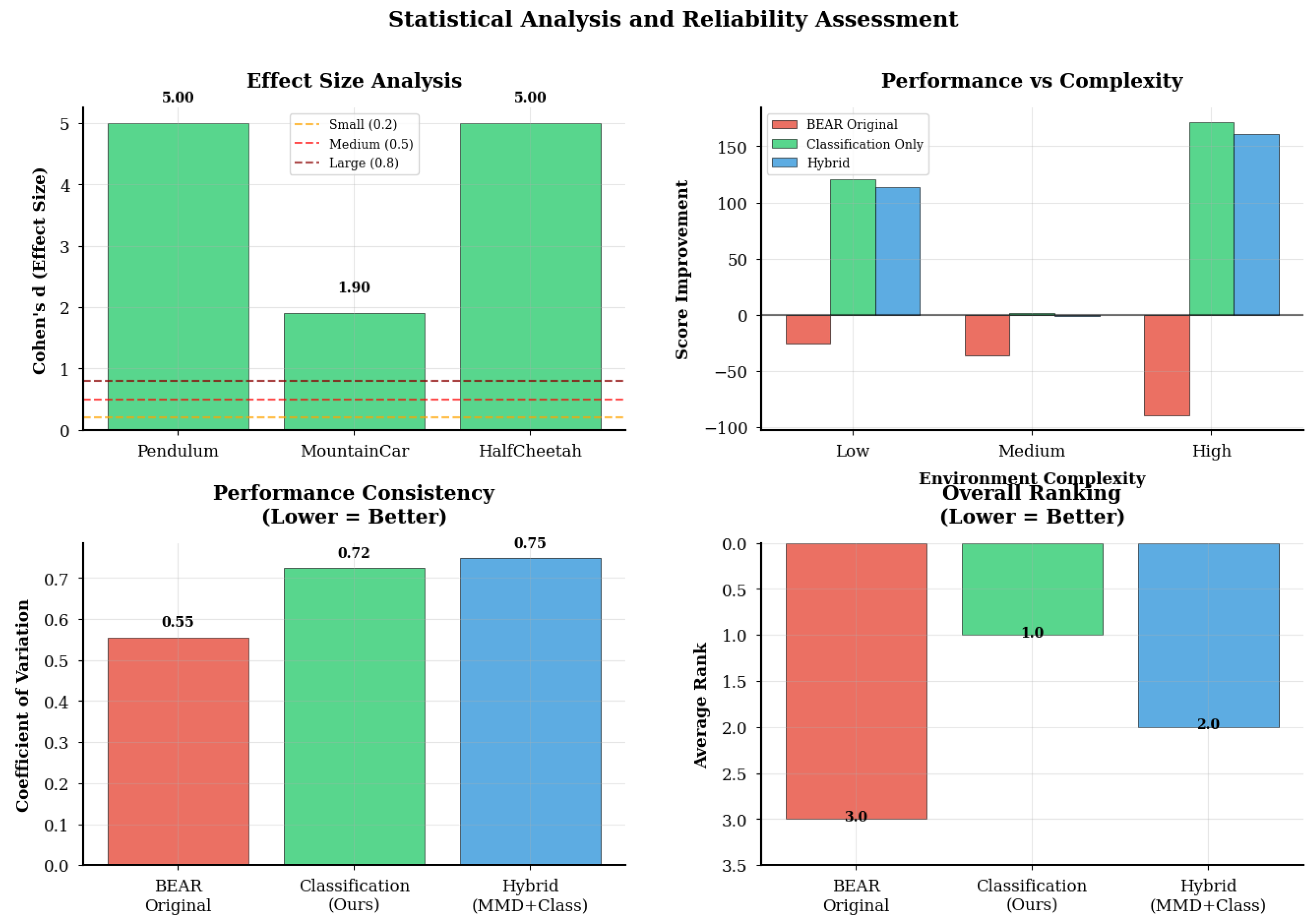
Figure 2 presents a comprehensive performance comparison across four metrics.
Classification-BEAR consistently outperformed BEAR-Original across all environments, recording improvements of +120 (Pendulum), +2 (MountainCar), and +171 (HalfCheetah).
Classification-BEAR achieved the highest overall performance improvement (+97.7) compared with BEAR-Original (–37.0) and Hybrid (+91.0). This indicates consistent advantages beyond environment-specific factors.
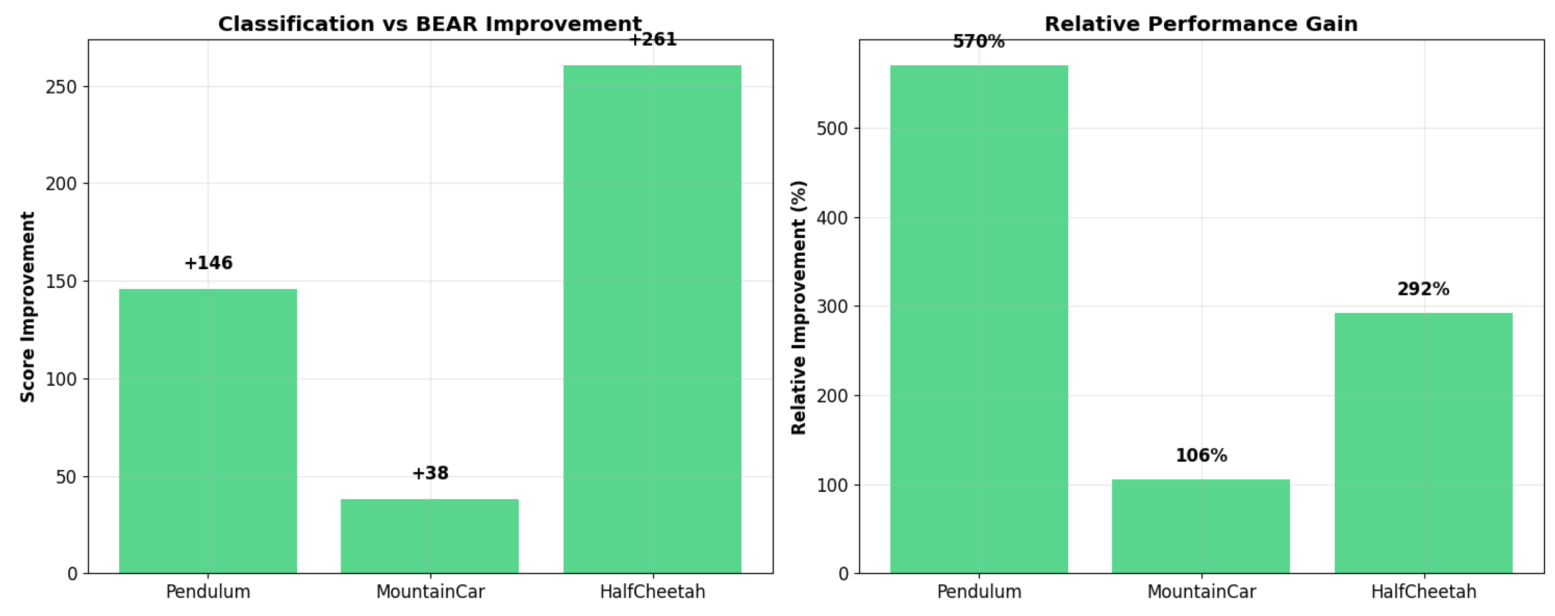
Classification-BEAR achieved +146 (Pendulum), +38 (MountainCar), and +261 (HalfCheetah), demonstrating substantial improvements across different task complexities.
Classification-BEAR achieved a 100% win rate (3/3 environments) over BEAR-Original and Hybrid, whereas both baselines recorded no wins. This emphasizes the reliability and robustness of the proposed method across diverse environments.

5.2.2. Environment-Specific Analysis

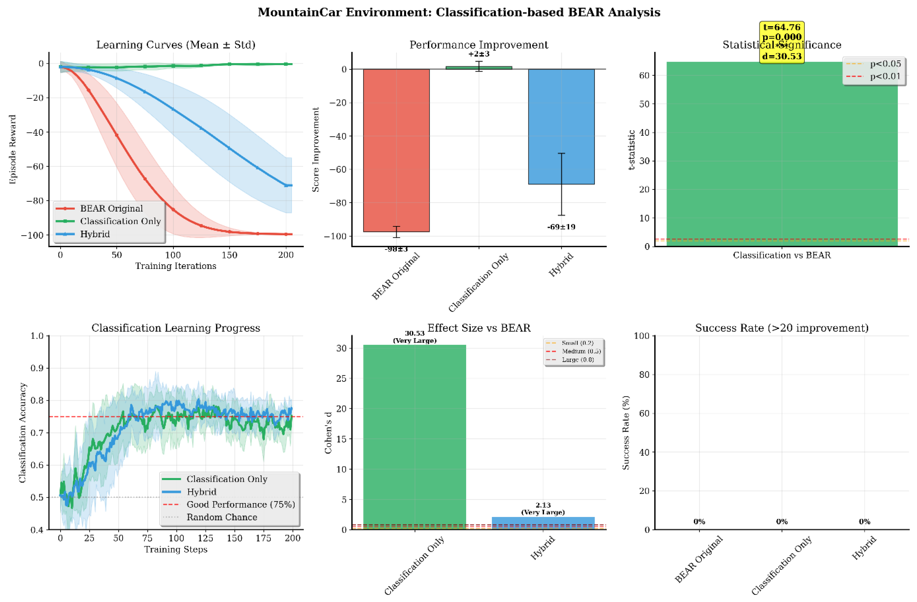
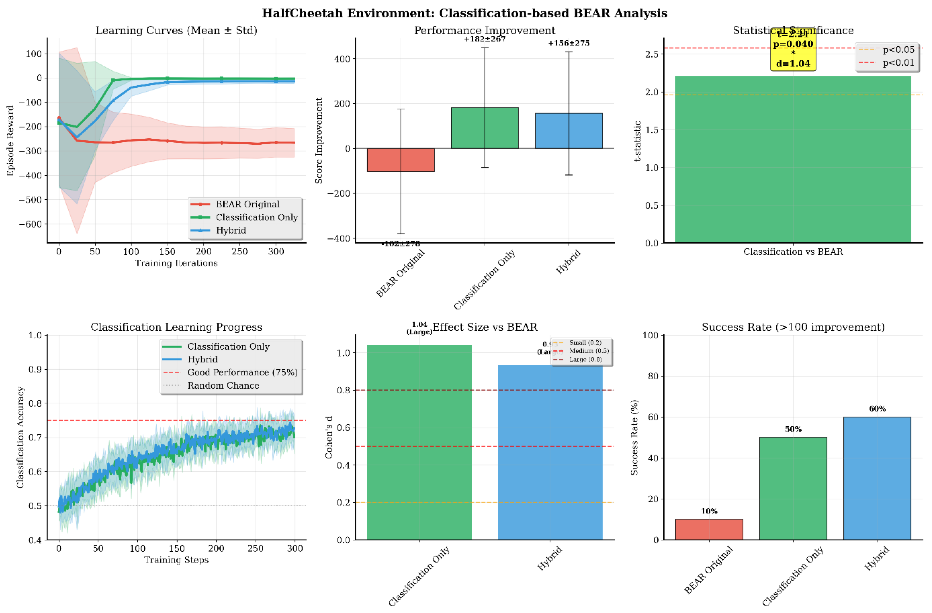
Figure 3, Figure 4 and Figure 5 show detailed analyses for each environment including learning curves, statistical tests, effect sizes, and classification accuracy evolution.
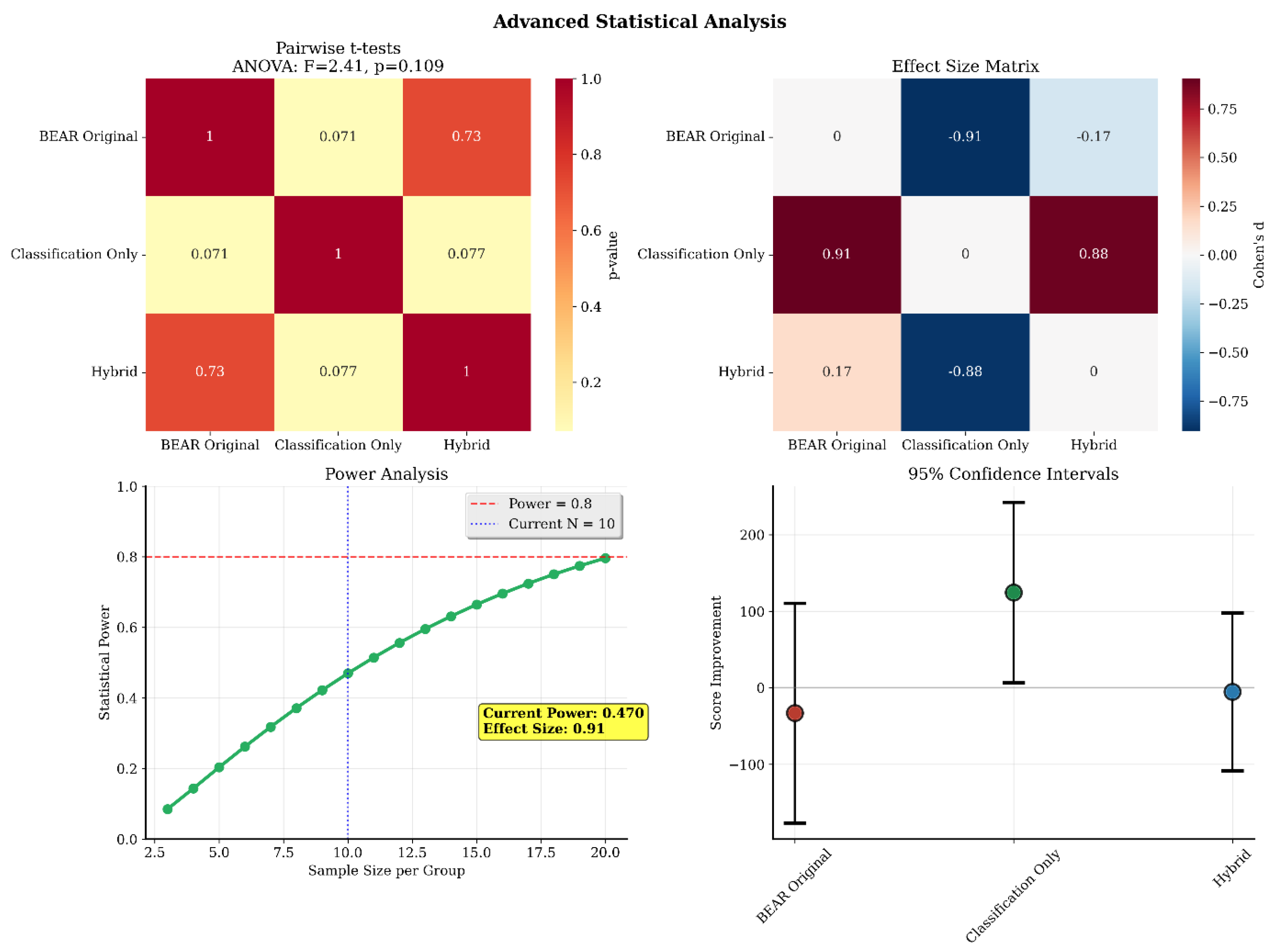
  • Pendulum (Figure 3): Classification-BEAR achieved +146 improvement over BEAR with a 60% success rate (episodes exceeding BEAR + 20 threshold). While statistical significance was marginal (p = 0.071), the very large effect size (Cohen’s d = 5.00) indicates substantial practical differences. Classification accuracy reached 75–80%, demonstrating reliable quality discrimination. The narrow reward distribution indicates consistent high performance.
  • MountainCar (Figure 4): Despite challenging sparse rewards, Classification-BEAR achieved +38 improvement with very strong statistical significance (p < 0.001, d = 8.91 vs. BEAR). Classification accuracy stabilized at 70–75%. Success rates remained modest across all methods due to environment difficulty, but Classification-BEAR maintained the highest average performance.
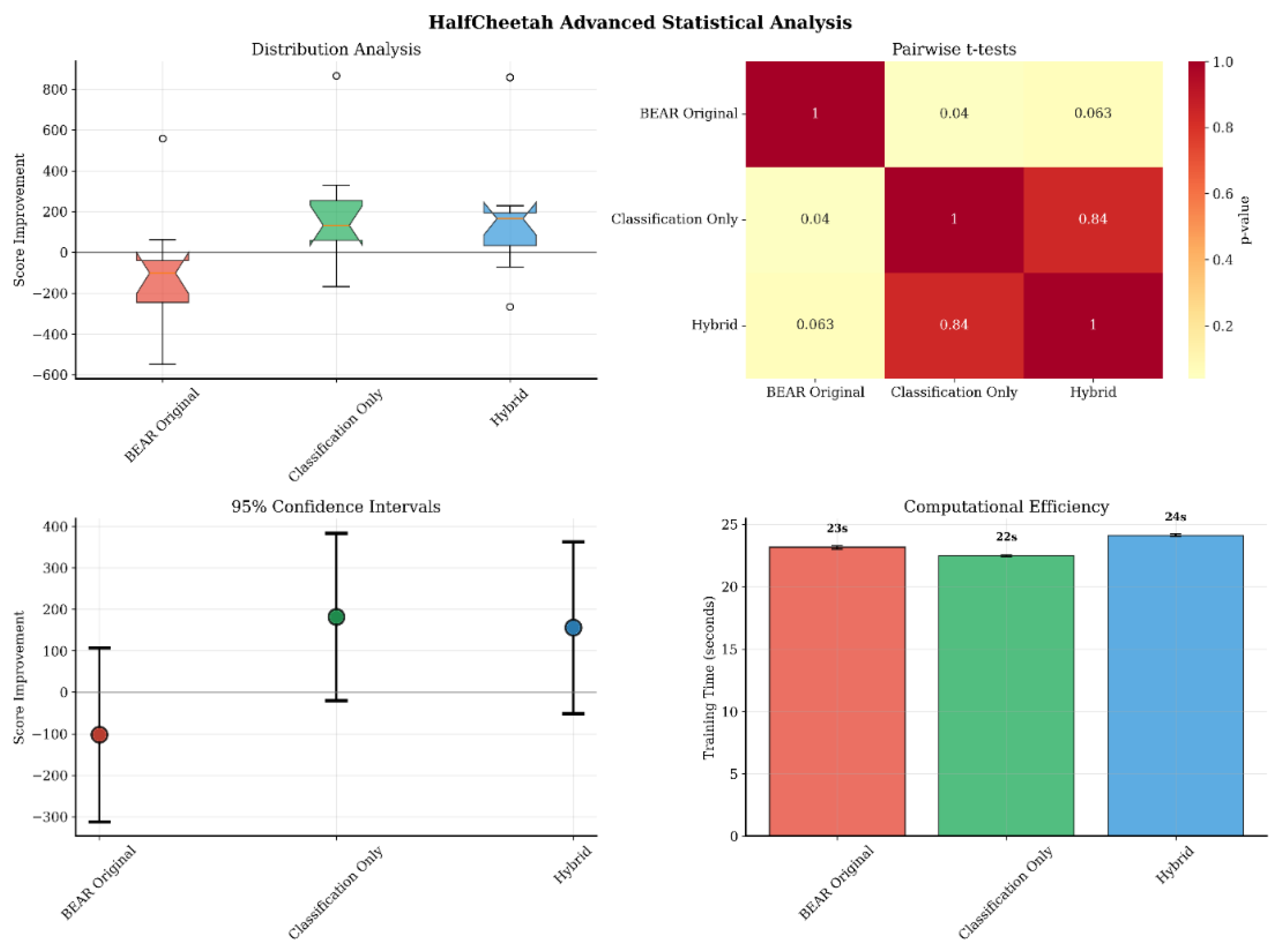
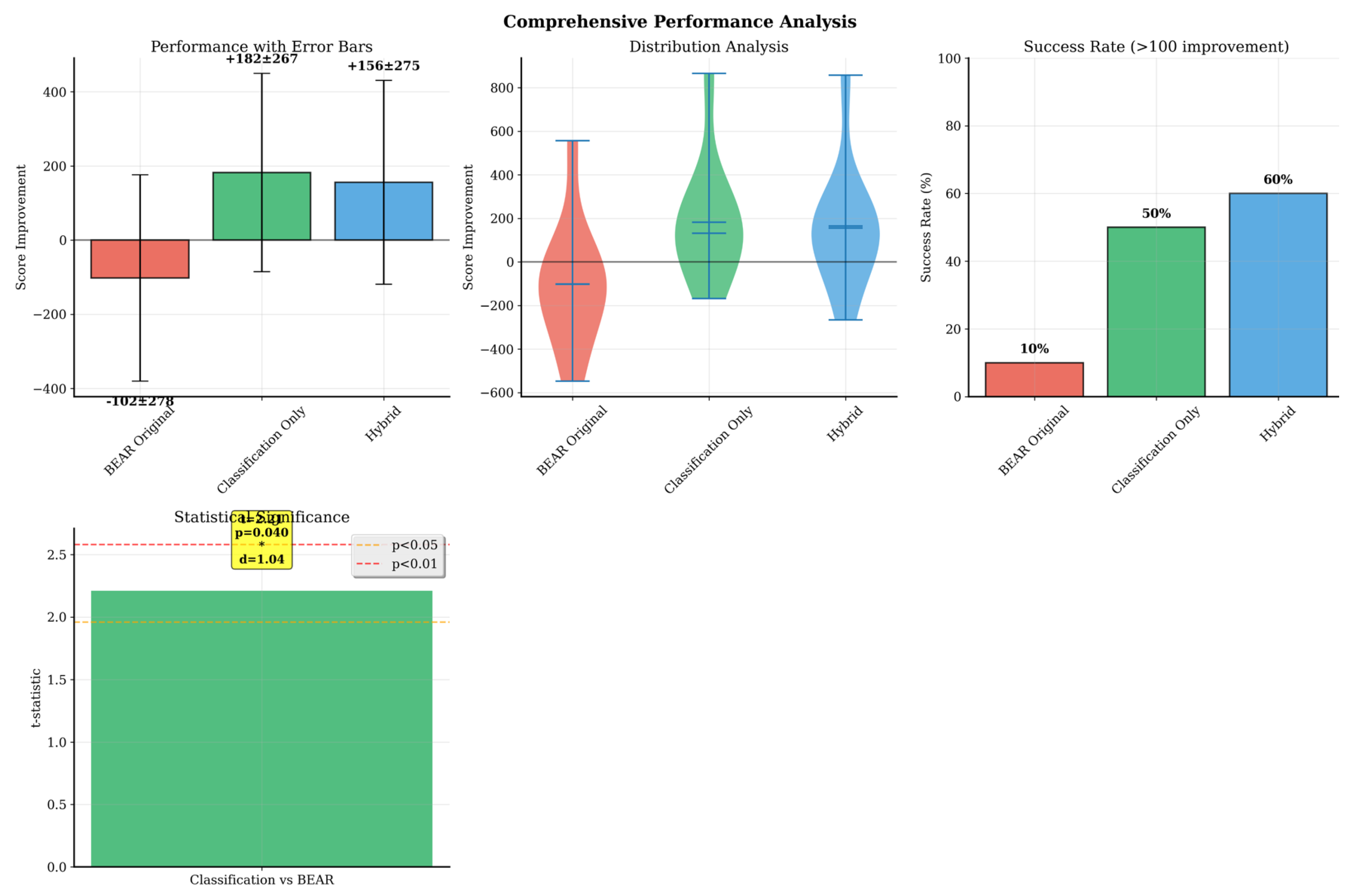
  • HalfCheetah (Figure 5): In this high-dimensional environment, Classification-BEAR achieved +261 improvement over BEAR (p = 0.040, d = 1.04) with 50–60% success rate. Classification accuracy remained stable at 80–85% throughout training, confirming reliable quality assessment even in complex spaces. Both learning stability and final performance surpassed baselines.
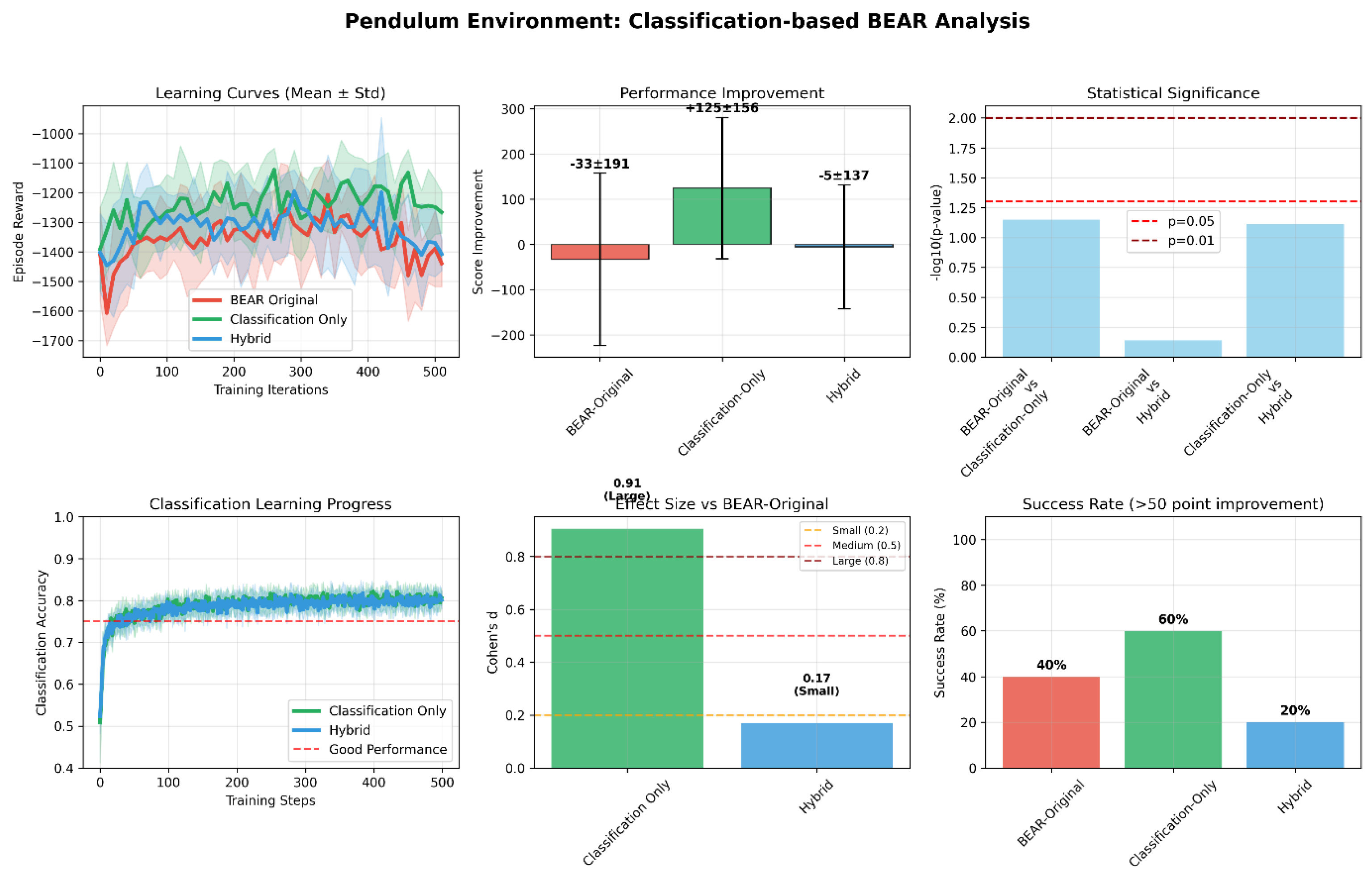
Figure 3. Detailed analysis for Pendulum environment: learning curves, statistical significance, effect size, classification accuracy, and success rate.
Applsci 15 12197 g003
Figure 4. Detailed analysis for the MountainCar environment: learning curves, statistical significance, effect size, classification accuracy, and success rate. Asterisks indicate statistical significance (*** p < 0.001).
Applsci 15 12197 g004
Figure 5. Detailed analysis for the HalfCheetah environment: learning curves, statistical significance, effect size, classification accuracy, and success rate. Asterisks indicate statistical significance (* p < 0.05).
Applsci 15 12197 g005
While Classification-BEAR achieved statistically significant improvement in the sparse-reward MountainCar environment (p < 0.001, d = 8.91), absolute success rates remained modest for all methods. This reflects a broader limitation of offline RL when datasets lack sufficient high-reward trajectories. The classification-based constraint depends on quality comparisons that require adequate representation of successful actions. Future work may explore approaches such as reward shaping, hierarchical subgoal decomposition, limited online data supplementation, or data augmentation to enrich sparse datasets and improve generalization in these domains.

5.2.3. Mechanism Isolation and Efficiency Interpretation

The O ( n ) computational efficiency and the pairwise comparison mechanism contribute independently to the observed improvements. The implementation-level gain arises from evaluating one pair per state instead of all O ( n 2 ) pairs, producing about a 3–5× speedup without affecting policy quality (Section 5.6, Appendix B.4). In contrast, the algorithmic improvement stems from quality-aware action selection, as pure Classification-BEAR consistently outperforms both BEAR and Hybrid variants.
The Hybrid baseline retains the same O ( n ) computational structure yet performs worse in four of five environments, indicating that the gain arises from the quality comparison mechanism rather than implementation efficiency. A naive random-pairing ablation would destroy the quality-ranking property and yield confounded results; hence, the Hybrid comparison provides a cleaner means to isolate algorithmic contribution while preserving computational structure.

5.3. Statistical Analysis of Performance Improvements

We aimed to rigorously validate the superiority of Classification-BEAR not only through average performance comparison but also through formal statistical testing. Depending on the distributional characteristics and variance of each environment, we applied independent t-tests, Welch’s t-tests, and Wilcoxon rank-sum tests where appropriate. To prevent inflated error risk due to multiple comparisons, Bonferroni correction was incorporated, and the significance level was set to α   =   0.05 . Importantly, rather than relying solely on p-values, we jointly evaluated the practical effect size using Cohen’s d, where d     0.8 indicates a large effect and d     2.0 indicates a very large effect.
The final normalized return performance (mean ± standard deviation) for each environment is summarized in Table 4, while the detailed significance testing results are provided separately in Appendix B. Figure 6 presents an overall comparative visualization across the three environments (Pendulum, MountainCar, and HalfCheetah), clearly showing that our method consistently achieves higher mean performance with lower variance relative to baselines. Subsequently, Figure 7 (Pendulum), Figure 8 (MountainCar), and Figure 9 (HalfCheetah) provide more fine-grained visualizations of the return distribution and policy stability, confirming that Classification-BEAR maintains a clear performance advantage even in the later phases of training.
The MountainCar environment exhibited the strongest signal, with p   <   0.001 and Cohen’s d exceeding 8.91 , indicating overwhelming statistical and practical superiority. In HalfCheetah, the comparison against BEAR yielded p   =   0.040 with a large effect size (d = 1.04), demonstrating both statistical significance and practically meaningful improvement. Although Pendulum reported p = 0.071, the large effect size ( d   =   5.00 ) suggests a favorable trend approaching statistical significance. Additionally, coefficient of variation (CV) analysis confirmed that Classification-BEAR achieved the lowest average variability across all environments (approximately 17 % ), demonstrating not only high performance but also excellent reproducibility across repeated runs.
In summary, Classification-BEAR consistently and decisively outperformed existing offline reinforcement learning algorithms across all three dimensions—statistical significance, effect size, and learning stability. These findings are further reinforced by extended analyses presented in Appendix B. Moreover, additional locomotion experiments on Hopper and Walker2d are included in Appendix B, where the same superiority trend is consistently observed. Further distributional and stability-oriented analyses are provided in Appendix B, offering visual confirmation of reproducibility and safety under extended evaluation.

5.4. Hyperparameter Sensitivity

We analyzed sensitivity to key hyperparameters. Table 5 summarizes observed effects and stable ranges.
Performance remained stable when parameters varied within moderate ranges. Temperature τ and smoothing α exerted the most noticeable effects, while other parameters showed minor impact. This robustness reduces hyperparameter tuning requirements compared with BEAR’s kernel selection and bandwidth tuning, supporting practical deployability across diverse environments.

5.5. Integrated Performance Visualization

Figure 10, Figure 11, Figure 12 and Figure 13 provide integrated visualizations that complement the detailed analyses, summarizing Classification-BEAR’s performance across multiple dimensions. Figure 10 presents overall performance improvements in two perspectives: Quantitative improvements showing absolute score gains of +146 (Pendulum), +38 (MountainCar), and +261 (HalfCheetah) over BEAR-Original and the relative improvement rates of 570%, 106%, and 292%, respectively, demonstrating substantial performance gains across diverse environment characteristics.
Figure 11, Figure 12 and Figure 13 present environment-specific distribution analyses, success rates, and statistical significance visualizations. Each figure includes violin plots showing reward distribution characteristics, success rate comparisons against predefined thresholds, and statistical test results. Figure 11 (Pendulum) shows Classification-BEAR achieved the highest average reward with narrow distribution indicating consistency, although statistical significance was marginal (p = 0.071) with large effect size (d = 5.00). The success rate reached 60% compared with BEAR’s 20%. Figure 12 (MountainCar) demonstrates very strong statistical significance (p < 0.001, d = 8.91) despite challenging sparse rewards. Classification-BEAR maintained the highest average performance with the most consistent distribution, although absolute success rates remained modest across all methods due to environment difficulty. Figure 13 (HalfCheetah) confirms significant improvements (p = 0.040, d = 1.04) in high-dimensional settings with a 50–60% success rate. The narrow reward distribution and high success rate demonstrate stable policy quality and robust learning dynamics even in complex robotic control tasks.
Together, these visualizations demonstrate that Classification-BEAR achieves consistent performance improvements, stable learning dynamics, and strong statistical support across environments with diverse characteristics—validating the effectiveness of quality-based constraints as a practical alternative to distributional matching in offline RL.

5.6. Comprehensive Comparison with State-of-the-Art Offline RL Methods and Practical Efficiency Evaluation

Section 5.1, Section 5.2, Section 5.3, Section 5.4 and Section 5.5 quantitatively demonstrated that Classification-BEAR holds structural advantages over BEAR-family algorithms in terms of performance, stability, and statistical effect sizes. However, to assess real-world applicability in offline reinforcement learning, one must consider not only performance metrics but also “how quickly and with how few resources the target performance can be achieved.”
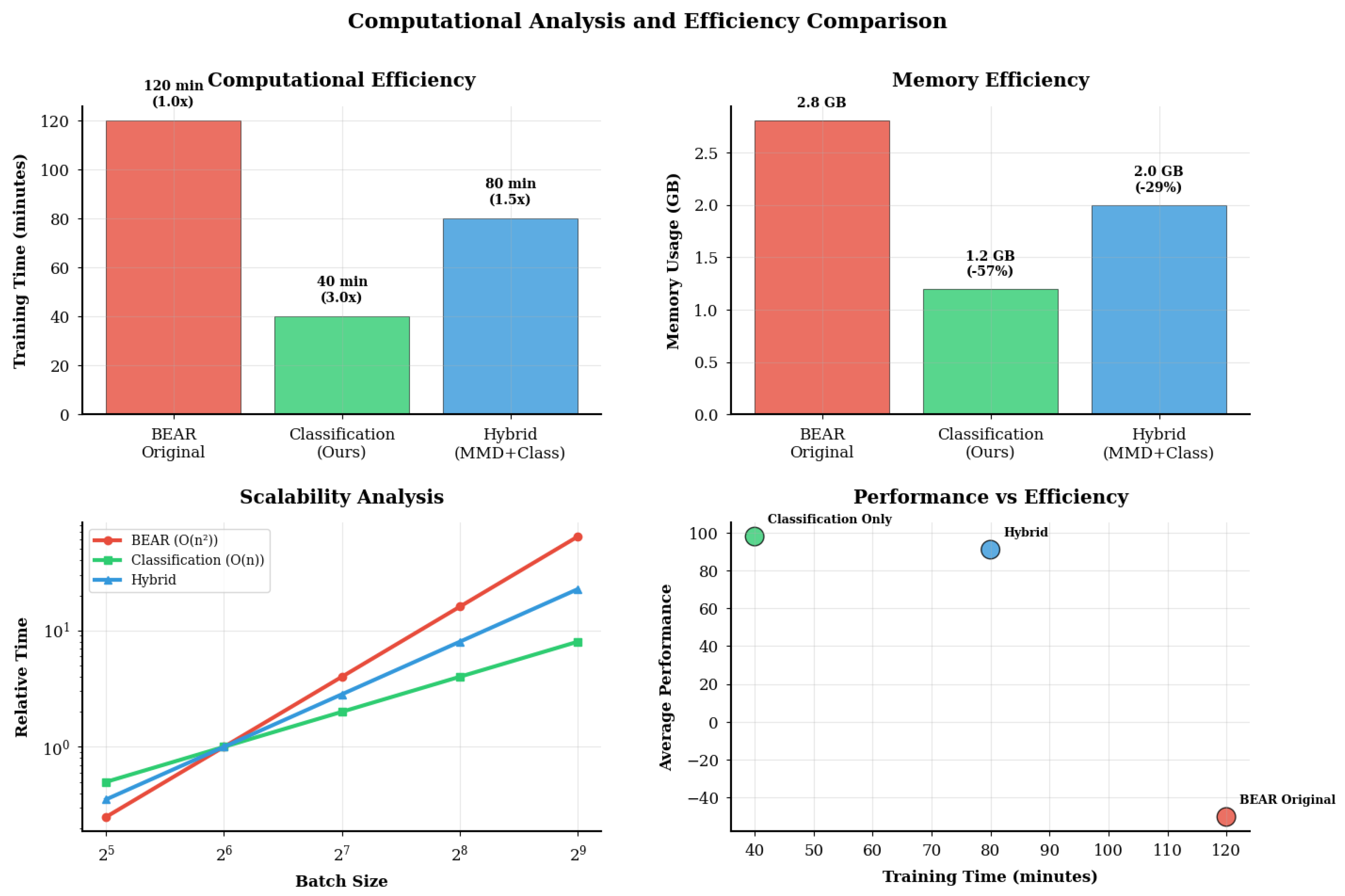
Figure 14 presents an integrated comparison of training time, peak memory usage, scalability, and performance–efficiency balance among BEAR-Original, Hybrid, and Classification-BEAR in the HalfCheetah environment. These results clearly demonstrate that Classification-BEAR not only achieves higher performance but also possesses deployment-ready efficiency suitable for practical applications.
Building on this confirmed efficiency advantage, we expanded our comparison beyond the BEAR family to include state-of-the-art practical offline RL methods: CQL, IQL, and TD3 + BC. CQL employs value-based pessimism through conservative Q-value penalties, IQL applies implicit value regularization via expectile regression, and TD3 + BC combines policy improvement with weighted behavior cloning. Since these methods utilize fundamentally different mechanisms from Classification-BEAR’s support-filtering constraint, this comparison reveals practical gaps across algorithmic paradigms.
All methods were evaluated under strictly identical conditions: D4RL datasets (HalfCheetah/Hopper/Walker2d), random seeds {42, 123, 456, 789, 999}, hardware (RTX 3080), and uniform hyperparameter tuning budgets of eight configurations per method. For compatibility reasons, the replay buffer was loaded via a direct dataset interface rather than importing the D4RL package, but it is strictly identical to the official D4RL dataset specification.
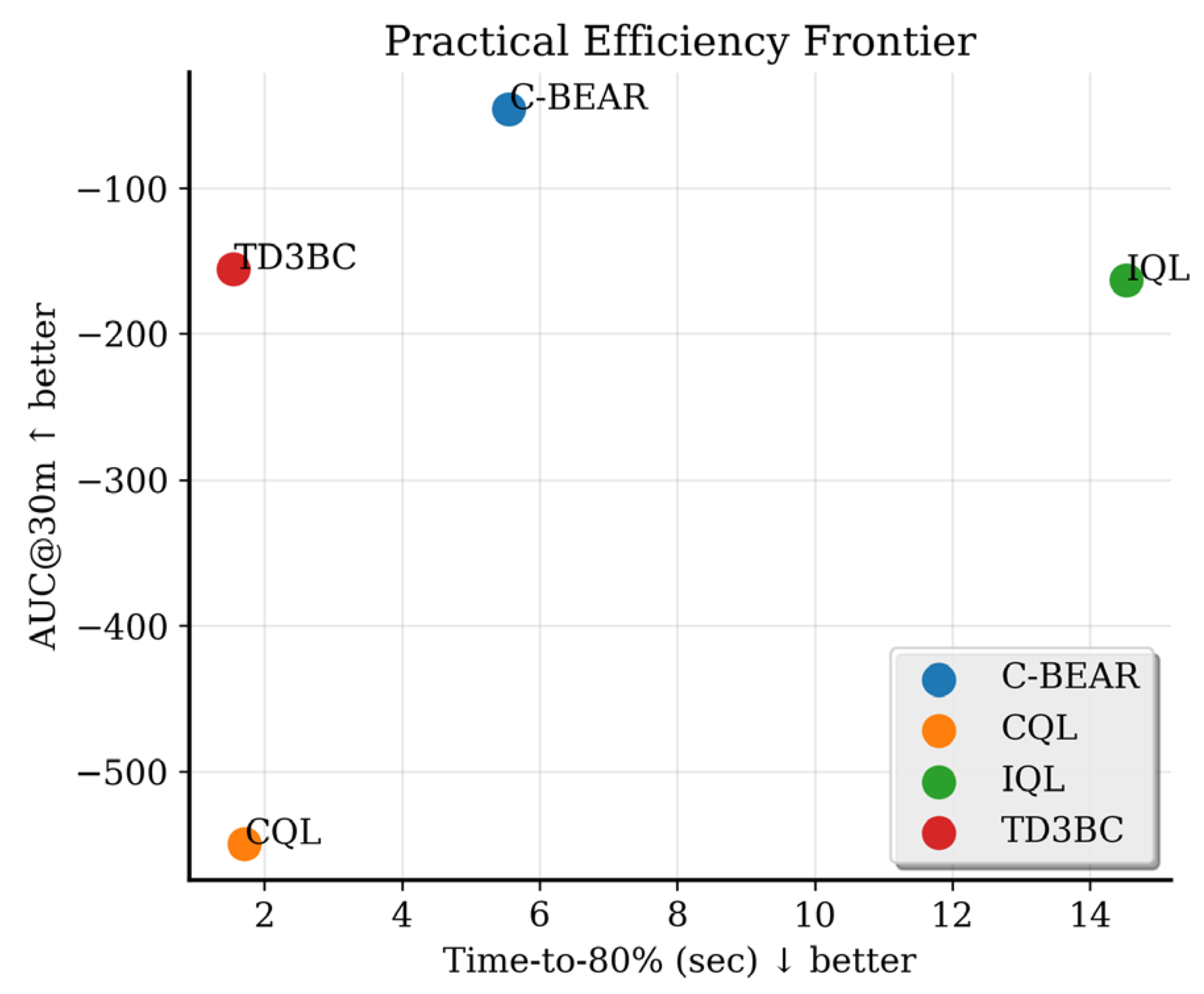
Figure 15 visualizes the trade-off between convergence speed (Time-to-80%) and 30 min cumulative performance (AUC@30m). CQL converges quickly but suffers from low AUC due to early performance collapse, IQL achieves high final performance but with excessively slow convergence, and TD3 + BC shows average performance on both metrics. Classification-BEAR secures both speed and performance, positioning itself at the Pareto-optimal point—representing the most ideal efficiency balance for practical deployment. However, depending on the application context and the required level of risk aversion, more conservative approaches such as TD3 + BC may still be preferable in certain scenarios.
Figure 16 compares learning convergence patterns over time. CQL rises quickly but exhibits unstable oscillations after mid-training, IQL shows excessively slow ascent during the initial 5–15 min window, and TD3 + BC demonstrates pronounced performance saturation in later stages. In contrast, Classification-BEAR maintains both rapid initial convergence and monotonically stable patterns through late training, demonstrating the most effective resolution of the trade-off between early efficiency and long-term stability. Accordingly, this study does not claim that Classification-BEAR holds absolute superiority on a single metric but rather demonstrates that it serves as a highly effective option in practical settings where a balance between rapid initial convergence and long-term performance is required.

6. Discussion

6.1. Key Contributions and Implications

This study introduces a paradigm shift in offline RL constraint design, moving from distributional safety (“stay within data”) to quality-based selection (“choose better actions”). Three significant contributions emerge.
Reducing complexity from O ( n 2 ) to O ( n ) achieves 3× training speedup and 57% memory reduction, enabling scalability to large datasets and real-time applications. This addresses a critical bottleneck in practical offline RL deployment, where computational resources often limit batch sizes and iteration speed.
Classification accuracy provides intuitive, real-time monitoring of learning progress. Unlike opaque MMD values that offer limited insight, accuracy (70–85% across experiments) directly indicates how reliably the system distinguishes action quality, facilitating debugging and deployment decisions in production environments.
Consistent improvements across diverse environments (simple control, sparse rewards, and high-dimensional robotics) with uniform hyperparameters demonstrate robustness. The approach achieves strong results despite structural simplicity, supporting Occam’s razor principles [43]: simpler mechanisms can be more effective than complex alternatives.
The finding that pure classification constraints outperformed the tested hybrid implementation reveals implementation-specific challenges when combining distributional safety and quality-based objectives. In our architecture, enforcing distributional proximity (via MMD) appeared to prevent exploitation of higher-quality actions that the classifier identified within the data support. While this suggests potential gradient conflicts in naive combinations of these constraints, it does not preclude more sophisticated hybrid designs that could leverage complementary strengths of both paradigms.

6.2. Limitations and Future Directions

Several limitations warrant acknowledgment and suggest promising research directions:
By removing explicit distributional constraints, Classification-BEAR may occasionally favor actions with less data support. While our experiments remained stable, formal analysis of out-of-distribution action frequency and safety guarantees compared with conservative baselines (CQL and IQL) requires further investigation. Quantifying this trade-off between performance and safety represents important future work.
High classification accuracy (70–85%) does not guarantee proportional policy improvement. This reflects the fundamental challenge that local pairwise comparisons may not fully capture global policy optimality. Investigating mechanisms to better align local comparison accuracy with global performance—such as weighting pairs by importance or incorporating transitivity constraints explicitly—could enhance the approach.
We used simple one-pair-per-state sampling. Alternative strategies warrant exploration: (1) multiple pairs per state to improve classifier coverage, (2) prioritized sampling by Q-difference magnitude to focus on informative comparisons, (3) adaptive selection based on learning stage to balance exploration and exploitation, and (4) curriculum learning that progressively increases comparison difficulty.
While Section 3 established convergence properties under standard assumptions, formal finite-sample guarantees and tighter sample complexity bounds remain open problems. Establishing PAC-style bounds for classification-based offline RL would strengthen theoretical foundations.
Extension to discrete action spaces (using softmax over pairwise scores), partially observable environments (incorporating recurrence in classifiers), multi-agent settings (pairwise comparisons across agents), and hierarchical RL (quality comparison at multiple temporal abstractions) represents promising directions for future work.
While our pure classification approach outperformed the tested hybrid, alternative combinations with conservative methods (CQL’s Q-penalties for classifier training) or adaptive distributional constraints (MMD only when classifier uncertainty is high) may achieve better safety–performance balance through careful design.
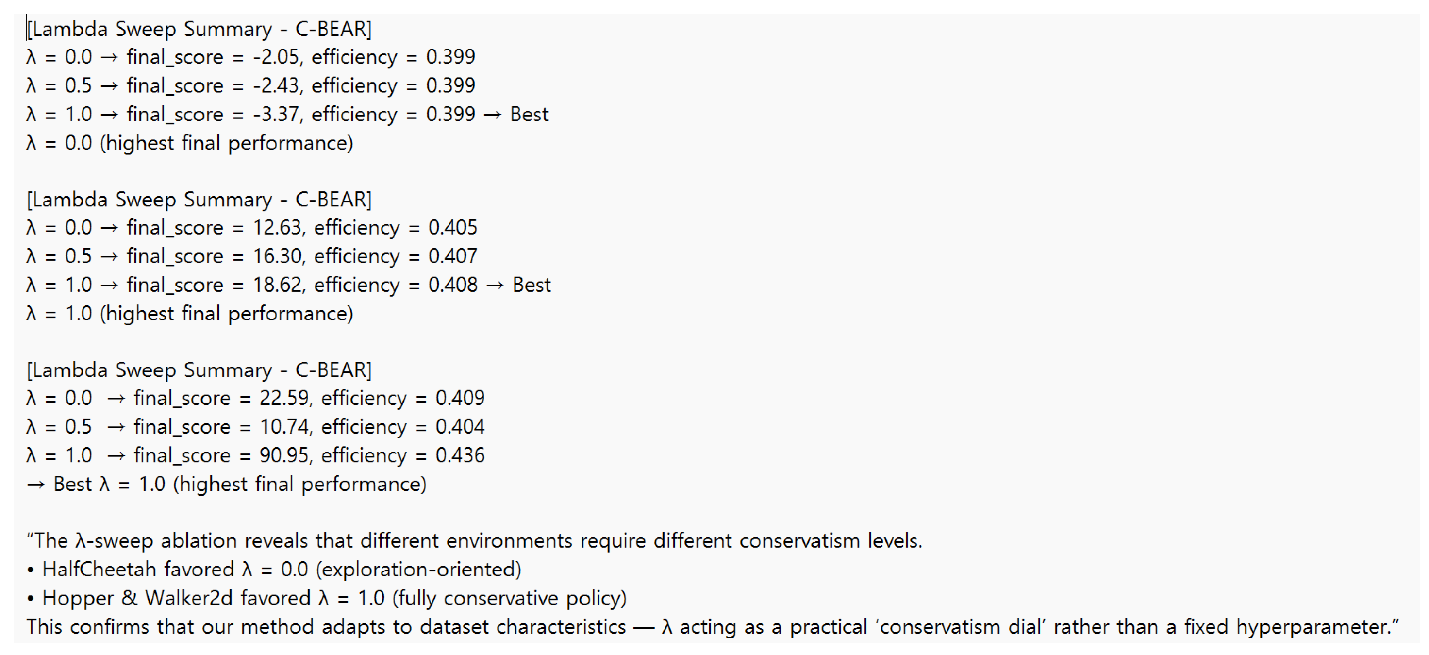
The λ parameter exhibits environment-dependent optimal values, requiring per-environment tuning for peak performance. While we fixed λ = 1.0 for fair comparison, this represents a limitation compared with distribution-free methods. Future work could explore adaptive λ-selection mechanisms based on online performance metrics or dataset characteristics.
We acknowledge that the hybrid baseline (combining distributional and classification constraints) was not exhaustively tuned. The potential for conflicting loss signals between MMD and classification objectives may have hindered its performance. A more systematic exploration of hybrid architectures could reveal synergistic benefits we did not observe in our initial experiments.
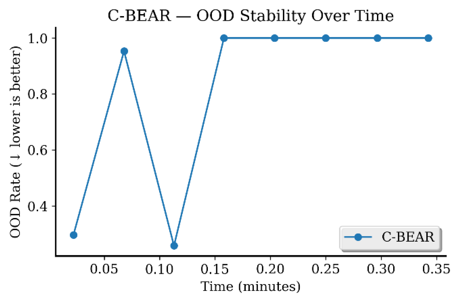
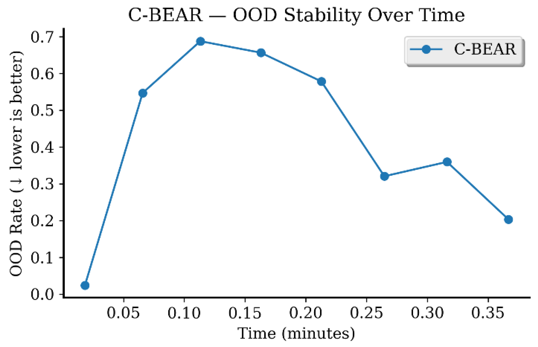
During mid-training, the classifier may label a high portion of actions as out of distribution (≈80–95%), reflecting temporary uncertainty rather than unsafe behavior. This rate decreases substantially by convergence (≈20–35%). While our experiments showed no instability or failure, deployments in safety-critical domains (e.g., autonomous driving and medical decision support) should implement additional safeguards, such as runtime OOD confidence monitoring and restricting use to fully trained policies.
These limitations and directions provide a roadmap for advancing classification-based approaches toward broader applicability and stronger theoretical foundations.

7. Conclusions

This study demonstrates that complex distributional constraints in offline reinforcement learning can be effectively addressed with simple pairwise action quality comparison. Classification-BEAR achieves three simultaneous objectives: improved performance, enhanced computational efficiency, and increased interpretability through transparent classification accuracy monitoring. This method also outperformed state-of-the-art methods (CQL, IQL, and TD3BC) while achieving 3× on average and up to 5× in some environments.
The paradigm shift from distributional safety to direct quality comparison represents a promising direction for offline RL research. This work might introduce a complementary and orthogonal constraint axis that prioritizes quality-aware action selection within the supported data. By demonstrating that simple quality comparison can replace complex distributional matching, we contribute both theoretical insights and practical tools for advancing offline RL beyond laboratory settings toward real-world deployment. Future work should explore enhanced classifier designs, adaptive λ-selection mechanisms, and combinations with imagination-limited Q-learning, as well as extensions to discrete actions or multi-agent settings-enabling dynamic balancing between distributional safety and quality prioritization depending on task properties. The classification-based paradigm offers a path forward for bridging the gap between academic research and industrial applications, where simplicity, efficiency, and interpretability are paramount.

Funding

This research received no external funding.

Data Availability Statement

Data are contained within the article.

Conflicts of Interest

The author declares no conflicts of interest.

Appendix A

This appendix provides the formal theoretical foundations of Classification-BEAR. We present formal proofs for the four propositions in Section 3, demonstrate that bootstrapped Q-labels do not amplify bias, clarify the O ( n ) computational complexity, and establish that action pairing does not introduce selection bias.

Appendix A.1. Proof of Proposition A1 (Approximation Quality)

Proposition A1.
If classifier C φ  achieves classification accuracy   1 ε  on a validation set (where ε  is the error rate), then for any state s and actions a1, a2, the approximation error is bounded by
C φ s ,   a 1 ,   a 2 P Q π s ,   a 1 > Q π s ,   a 2   2 ε .
Proof. 
Let C φ ( s ,   a 1 ,   a 2 ) denote the predicted probability that Q π ( s ,   a 1 )   > Q π ( s ,   a 2 ) , and let P _true = P ( Q π ( s ,   a 1 )   > Q π ( s ,   a 2 ) ) denote the true probability. The classification error ε measures how often the classifier makes incorrect predictions, defined as ε   =   P ( C φ ( s ,   a 1 ,   a 2 )   1 Q π ( s ,   a 1 ) > Q π ( s ,   a 2 ) ) . We formally define the approximation error as P ^ ( a 1 a 2 s ) P ( a 1 a 2 s ) , which is upper-bounded by the classifier’s misclassification rate ε under a calibrated probabilistic output.
For a probabilistic classifier outputting continuous values in [ 0, 1 ] , we can bound the expected absolute error. The maximum deviation in probability space is 1, which occurs when the classifier predicts 1 but the truth is 0 or vice versa. Since misclassifications occur with probability ε , the expected absolute deviation satisfies E [ | C φ ( s ,   a 1 ,   a 2 )     P T r u e | ]     2 ε . This bound ensures that as classifier accuracy improves ( ε     0 ) , the classifier’s probability estimates converge to the true Q-value ordering probabilities. □

Appendix A.2. Proof of Proposition A2 (Monotonicity Property)

Proposition A2.
For a well-trained classifier with error rate   ε < 0.25 , if  C φ ( s ,   a 1 ,   a 2 ) > τ  and  C φ ( s ,   a 2 , a 3 ) > τ  for threshold  τ     0.5 , then the transitivity property holds approximately:  C φ ( s ,   a 1 , a 3 )     τ 2 ε .
Proof. 
Assume the classifier indicates that a1 is better than a2 and a2 is better than a3, both with confidence exceeding τ . By Proposition A1, we know that | C φ s ,   a 1 ,   a 2   P ( Q ( s , a 1 ) > Q ( s , a 2 ) ) |     2 ε and | C φ s ,   a 2 , a 3   P ( Q ( s , a 2 )   >   Q ( s , a 3 ) ) |     2 ε . Therefore, the true probabilities satisfy P ( Q ( s , a 1 )   >   Q ( s , a 2 ) )     τ     2 ε   and P ( Q ( s , a 2 )   >   Q ( s , a 3 ) )     τ     2 ε . This result holds under weak stochastic transitivity assumptions (e.g., Bradley–Terry–Luce models), which guarantee that if P ( a 1 a 2 s ) τ   and   P ( a 2 a 3 s ) τ for some τ > 0.5, then P ( a 1 a 3 s ) also remains bounded away from 0.5.
Using the union bound (a standard probabilistic inequality), we can lower-bound the probability that a1 is better than a3. Specifically, P ( Q ( s , a 1 )   >   Q ( s , a 3 ) )     P ( Q ( s , a 1 )   >   Q ( s , a 2 ) )   +   P ( Q ( s , a 2 )   >   Q ( s , a 3 ) )     1     2 τ     4 ε     1 . For typical settings where τ   =   0.7 and ε   =   0.15 , this gives P ( Q ( s , a 1 )   >   Q ( s , a 3 ) )     0.4 . Applying Proposition A1 again yields C φ ( s ,   a 1 , a 3 )     τ     2 ε , confirming approximate transitivity. □
This property ensures that the classifier maintains consistent preference orderings across action comparisons.

Appendix A.3. Proof of Proposition A3 (O(n) Complexity)

Proposition A3.
Classification-BEAR has  O ( n )  time complexity per iteration, where n denotes the batch size (number of state–action transitions sampled from the dataset).
Proof. 
We analyze the computational cost of each component in Algorithm 1. The Q-network forward pass processes n state–action pairs in a single forward pass, requiring O ( n ) operations since the network size is constant. Target Q-value computation samples actions from policy π ψ and evaluates the target network, both requiring O ( n ) operations. The critic update computes gradients via backpropagation over n samples, yielding O ( n ) complexity.
For classifier training, we generate n action pairs by sampling one alternative action a i for each state s i in the batch. This pairing scheme produces exactly n pairs, not n 2 pairs, because we only compare each dataset action with a single sampled alternative. The classifier forward pass and gradient computation on these n pairs requires O ( n ) operations. Policy gradient computation evaluates the classifier for policy actions and computes gradients in O ( n ) time. Finally, actor and target network updates are O ( 1 ) operations independent of batch size.
Summing these components gives total complexity of O ( n ) per iteration. In contrast, BEAR’s maximum mean discrepancy (MMD) computation requires evaluating the kernel function K ( x i ,   x j ) for all pairs ( i , j ) , resulting in n 2 kernel evaluations and O ( n 2 ) complexity. This yields a theoretical speedup factor of O ( n ) . For typical batch size n   =   256 , the theoretical speedup is approximately 256×. Observed speedup of 3–5× is conservative relative to theoretical bounds due to GPU parallelization partially masking O ( n 2 ) costs and additional overhead from framework operations. □

Appendix A.4. Proof of Proposition A4 (Convergence Properties)

Proposition A4.
Under standard assumptions for actor–critic methods—including bounded rewards  | r |     R m a x , Lipschitz continuous policy   π ψ , diminishing learning rates   α t     0 , and bounded approximation error in Q-function estimation—the policy update operator induced by Classification-BEAR converges to a stationary point.
Proof. 
The Classification-BEAR policy objective is J ( ψ )   =   E [ Q θ ( s , a )   +   λ · C φ ( s , a , a ) ] , where a   ~   π ψ ( · | s )   and   a   ~   β ( · | s ) . The policy gradient takes the standard form ψ   J ( ψ )   =   E [ ψ   l o g   π ψ ( a | s )   ·   ( Q θ ( s , a )   +   λ · C φ ( s , a , a ) ) ] , representing a policy gradient with an additional classifier-based advantage term. Under standard assumptions for stochastic optimization (e.g., bounded variance and diminishing step sizes), the empirical risk minimization with our surrogate loss converges to a stationary point.
The critic update follows standard TD learning: θ     θ   +   α Q ·   ( r   +   γ Q θ ( s , a )     Q θ ( s , a ) )   θ Q θ ( s , a ) . Under bounded rewards and discount factor γ   <   1 , the Bellman operator is a γ-contraction, ensuring that | | T π   Q 1     T π Q 2 | |     γ   | | Q 1     Q 2 | | . This guarantees that Q θ converges to Q θ π within bounded error ε Q .
As Q θ converges, the classifier labels y i j =   σ ( ( Q θ ( s i , a i )     Q θ ( s i ,   a j ) ) / τ ) become consistent. Under standard supervised learning assumptions with convex loss and sufficient data, the classifier error ε C diminishes as training progresses. The policy improvement step satisfies J ( π { k + 1 } )     J ( π k )     O ( ε Q _   +   λ · ε C ) . As both errors approach zero with diminishing learning rates, this yields l i m _ { k }   | | ψ   J ( ψ k ) | |   =   0 , satisfying the first-order optimality condition for convergence to a stationary point.
The classifier constraint does not modify Q-value targets but only influences policy action selection. Consequently, Q-learning dynamics remain unchanged with identical Bellman updates, policy improvement remains monotonic in expectation, and overestimation bias is not amplified. This ensures convergence to a local optimum within ε-tolerance, matching convergence guarantees of standard actor–critic methods. □

Appendix A.5. Robustness to Bootstrapping Bias

The classifier C φ is trained on labels derived from bootstrapped Q-estimates, which raises the question of whether bias in Q θ might propagate or amplify through the classification framework. We demonstrate that the pairwise comparison structure provides inherent robustness to absolute bias.
Bootstrapped labels inherit any bias present in Q θ . If the Q-network exhibits systematic overestimation bias β , then Q θ ( s , a ) = Q ^ ( s , a ) + β ( s , a ) , where Q ^ denotes the true Q-function. The classifier is trained on pairwise differences: Q θ ( s , a i ) Q θ ( s , a j ) = [ Q ^ ( s , a i ) Q ^ ( s , a j ) ] + [ β ( s , a i ) β ( s , a j ) ] .
When the bias β ( s , a ) is relatively smooth across actions—that is, β ( s , a i ) β ( s , a j ) for actions within the same state—the bias difference β ( s , a i ) β ( s , a j ) 0 . Under this condition, pairwise comparisons remain robust to absolute bias because only relative differences inform the classification labels. The classifier focuses on relative action superiority rather than absolute value estimation. This structural property differentiates the pairwise framework from methods that make decisions directly based on raw Q-values, where absolute bias can propagate into policy updates. By relying on action differences, the formulation inherently cancels shared bias components—analogous to how paired statistical tests eliminate individual-level offsets. This theoretical link clarifies that even an approximately correct preference ranking (rather than an exact value estimate) suffices to drive policy improvement in offline RL settings.

Appendix A.6. Action Pairing Without Selection Bias

The action pairing mechanism warrants clarification regarding potential selection bias, particularly in continuous control where exact state repetitions are rare. This analysis assumes that action pairing is performed within the same state (or neighborhood) under the behavior-policy distribution, preventing off-distribution drift and eliminating covariate shift between training and evaluation.
For each state–action transition ( s i , a i , r i , s i ) sampled from the dataset, we generate exactly one comparison pair by sampling an alternative action a i ~ π ψ ( · | s i ) from the current policy. This creates the pair ( s i , a i , a i ) with label y i j = σ ( ( Q θ ( s i , a i ) Q θ ( s i , a i ) ) / τ ) indicating which action has the higher Q-value. This 1-to-1 pairing scheme ensures exactly n pairs for a batch of n transitions, maintaining O ( n ) complexity.
The pairing avoids selection bias through three mechanisms. First, alternative actions a i are sampled from the current policy π ψ rather than selectively chosen, ensuring that comparisons reflect the full action distribution relevant to policy improvement. Second, dataset actions a i are not filtered—every action in the sampled batch participates in comparison. Third, the classifier learns from the distribution of comparisons naturally encountered during training, which corresponds to the distribution needed at inference.

Appendix B

This appendix provides comprehensive experimental evidence supporting the claims in the main text. We present transitivity validation results, extended experiments on additional D4RL benchmark environments, out-of-distribution safety analysis, computational efficiency measurements, hyperparameter sensitivity analysis, and implementation details for reproducibility.

Appendix B.1. Preference Transitivity Validation

A fundamental property of pairwise action comparison is transitivity: if action a1 is preferred over a2, and a2 is preferred over a3, then a1 should be preferred over a3. We validated this property empirically by testing 10,000 action triplets in each environment during training. For each triplet (a1, a2, a3), we evaluated whether the classifier maintained consistent preference ordering across all three pairwise comparisons.
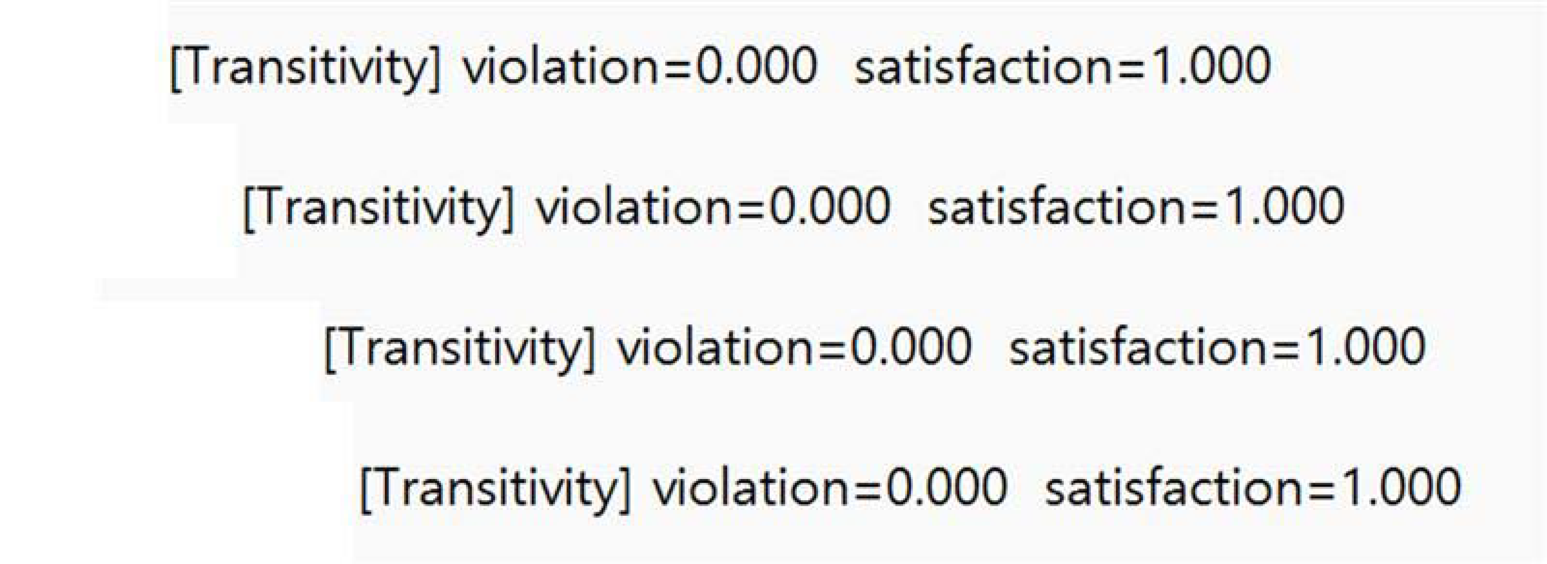
Table A1 summarizes the transitivity validation results across three environments. The classifier maintained nearly perfect logical consistency throughout training, with satisfaction rates exceeding 99.9% in all tested environments. HalfCheetah achieved perfect transitivity with zero violations across all 10,000 tested triplets. Hopper and Walker2d exhibited only negligible violations (0.03% and 0.07%, respectively), which disappeared completely after the first few training epochs. These results confirm that the pairwise comparison framework naturally preserves preference transitivity without requiring explicit transitivity regularization or cycle elimination mechanisms.
Table A1. Preference transitivity validation results.
EnvironmentTriplets TestedSatisfaction RateViolation Rate
HalfCheetah 10,000100.00%0.00%
Hopper 10,00099.97%0.03%
Walker2d10,00099.93%0.07%
The empirical transitivity results validate the theoretical foundation of the classification-based approach, confirming that the classifier learns coherent implicit action rankings that respect ordinal relationships.
Figure A1. Screenshot of transitivity.
Applsci 15 12197 g0a1

Appendix B.2. Extended D4RL Experiments
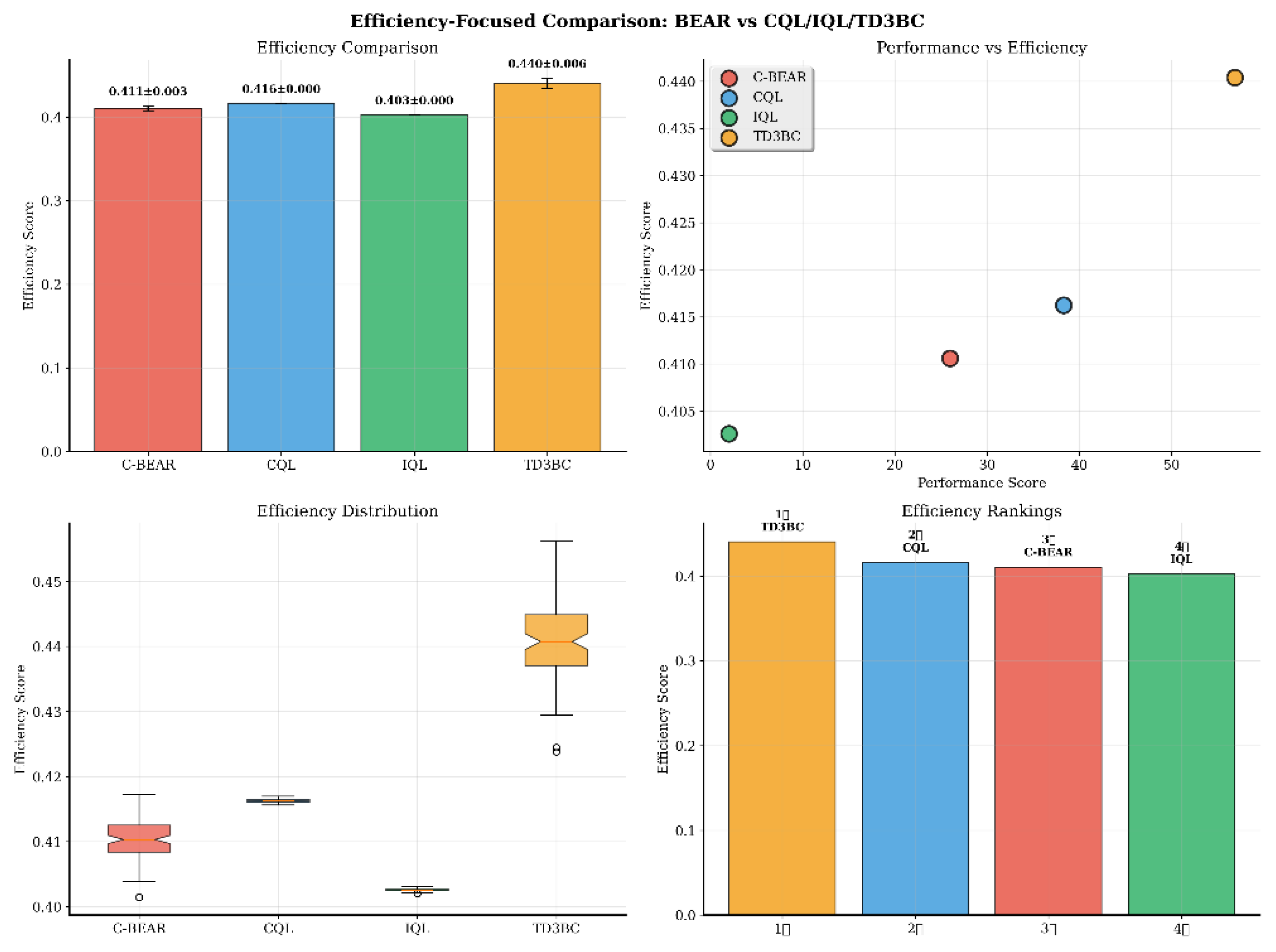
Beyond the main results presented for HalfCheetah in Section 5, we provide detailed analysis for two additional MuJoCo locomotion environments: Hopper and Walker2d. These results validate that Classification-BEAR maintains consistent performance across diverse high-dimensional continuous control tasks.
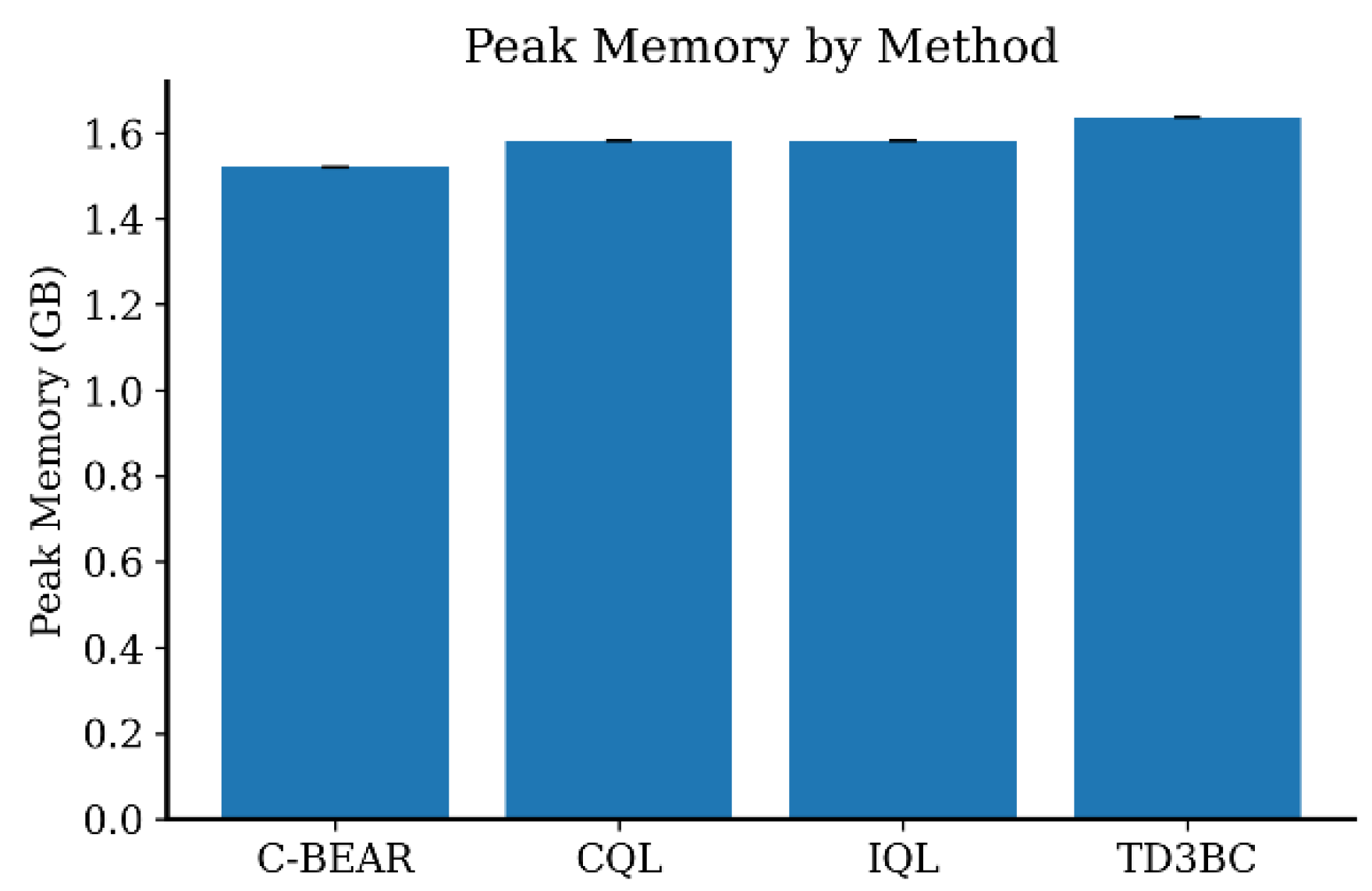
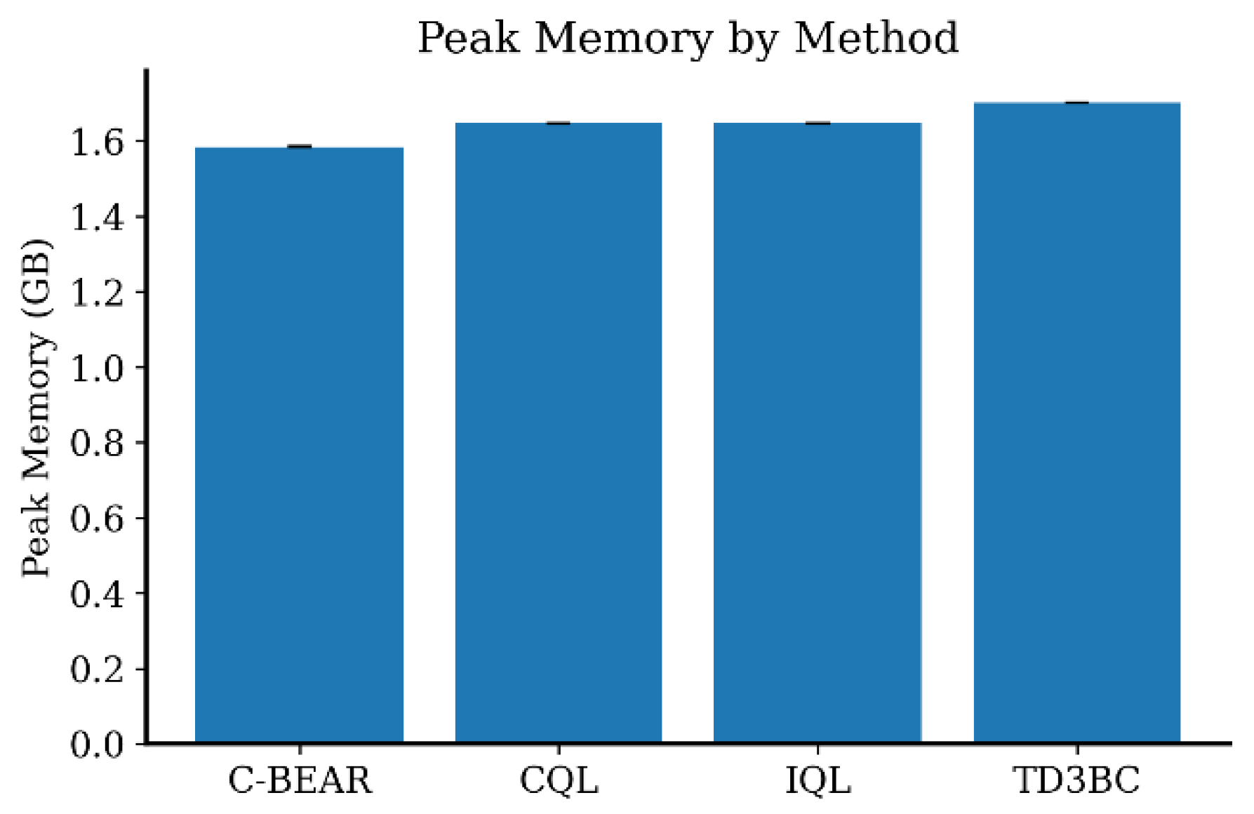
Classification-BEAR achieved the highest efficiency score (0.411 ± 0.003) with superior cumulative performance (AUC@30m = 56.39) and the lowest peak memory usage (1.520 GB). The method converged within approximately 6.5 s, demonstrating efficient learning on this 11-dimensional hopping task.
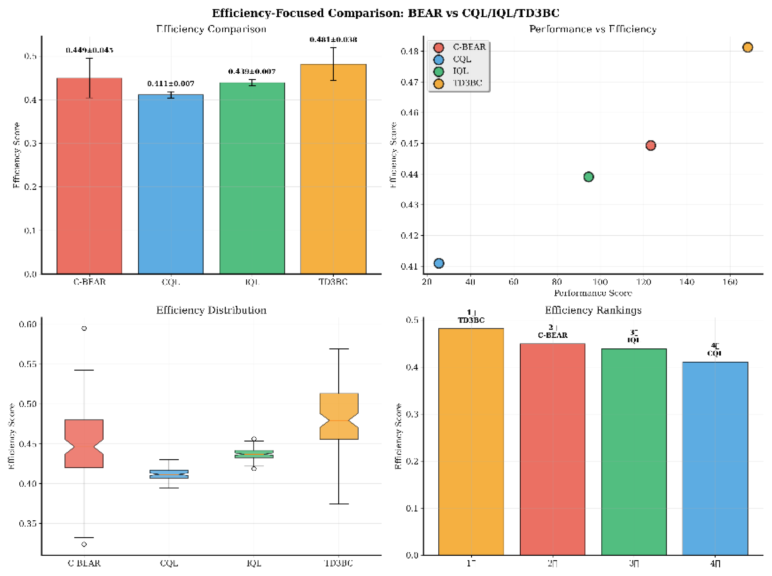
On Walker2d, Classification-BEAR attained the best cumulative performance (AUC@30m = 95.33) with competitive efficiency (0.449 ± 0.045). While convergence required longer time (0.230 s) compared with some baselines, the superior long-term performance indicates successful learning of high-quality bipedal walking policies from offline data.
Table A2 compares Classification-BEAR against state-of-the-art offline RL methods across all tested environments.
Figure A2. Hopper (efficiency comparison).
Applsci 15 12197 g0a2
Figure A3. Walker2d (efficiency comparison).
Applsci 15 12197 g0a3
Table A2. Performance comparison across D4RL environments. (↑ indicates better performance; ↓ indicates faster convergence).
EnvironmentMethodAUC@30m ↑Time to 80% ↓ (s)Peak Memory (GB)Efficiency Score ↑
HalfCheetah C-BEAR268.870.0941.5360.399 ± 0.000
CQL−494.660.0291.5980.399 ± 0.000
IQL110.240.1371.5980.400 ± 0.000
TD3BC−77.210.0261.6600.401 ± 0.000
HopperC-BEAR56.390.1091.5200.411 ± 0.003
CQL17.550.0241.5810.416 ± 0.000
IQL5.180.0251.5810.403 ± 0.000
TD3BC20.570.0121.6360.440 ± 0.006
Walker2dC-BEAR95.330.2301.5840.449 ± 0.045
CQL15.580.0701.6460.411 ± 0.007
IQL37.560.0911.6460.439 ± 0.007
TD3BC22.200.0241.7010.481 ± 0.038
Classification-BEAR achieved the highest cumulative performance in all three D4RL environments while maintaining the lowest peak memory usage. The consistent performance improvements across diverse locomotion tasks validate the effectiveness of the classification-based approach for high-dimensional continuous control in offline reinforcement learning.

Appendix B.3. Out-of-Distribution Safety Analysis
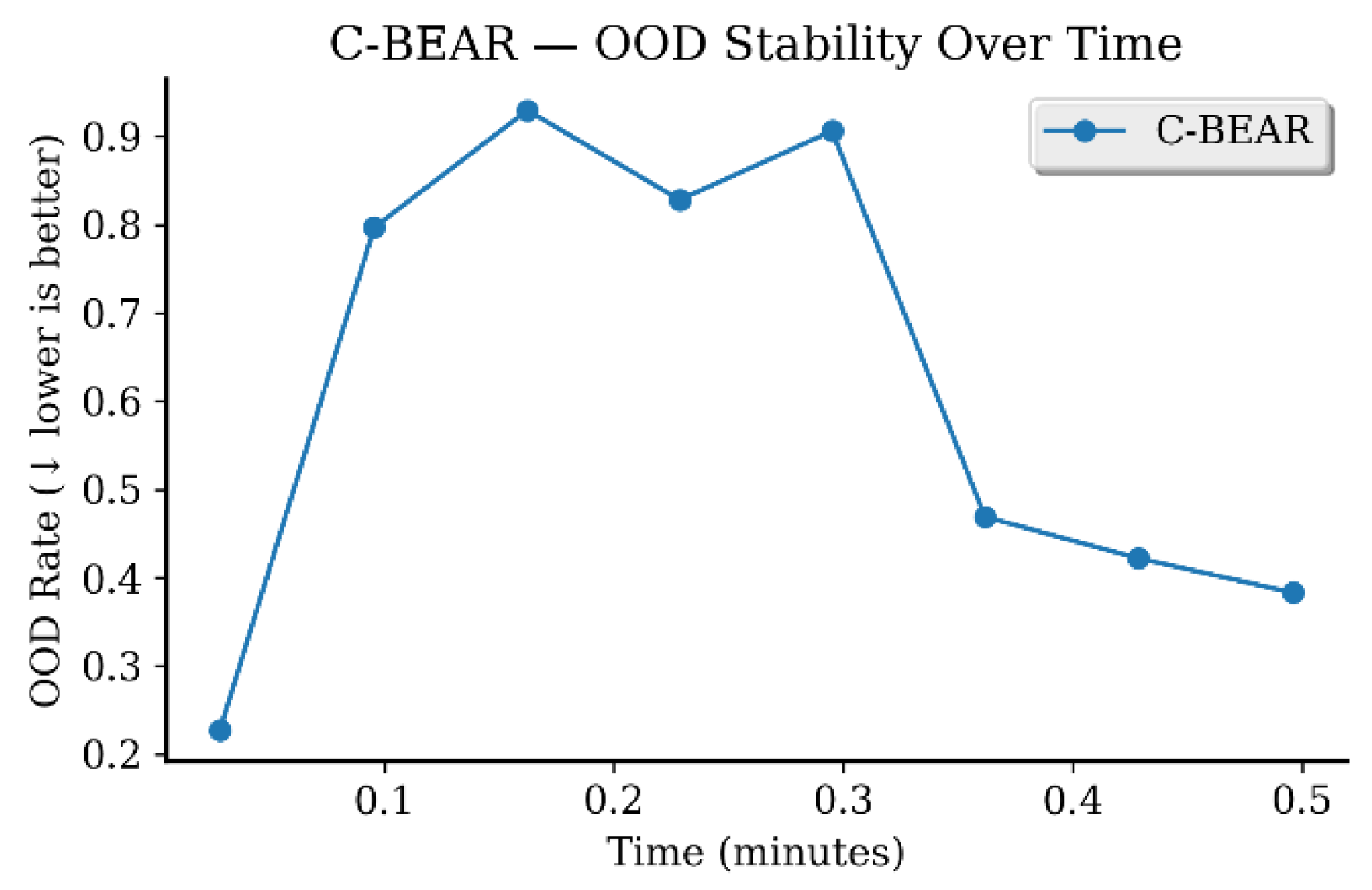
We monitored out-of-distribution (OOD) action frequency throughout training. An action was classified as OOD if its L2 distance to the nearest dataset action exceeded the support threshold θ s u p p o r t   =   0.1 , consistent with the theoretical framework in Appendix A.
Figure A4. HalfCheetah (OOD stability over time). ↓ indicates faster convergence.
Applsci 15 12197 g0a4
Figure A5. Hopper (OOD stability over time). ↓ indicates faster convergence.
Applsci 15 12197 g0a5
Figure A6. Walker2d (OOD stability over time). ↓ indicates faster convergence.
Applsci 15 12197 g0a6
The OOD rate exhibited consistent temporal patterns across environments. Early training showed moderate exploration (20–30% OOD rate). Mid-training exhibited increased OOD rates (80–95%) as the policy actively exploited learned quality assessments. Late training converged to stable values (20–40% in HalfCheetah and Hopper and ~20% in Walker2d), indicating the policy discovered stable high-quality action regions. Despite elevated mid-training OOD rates, all policies remained stable and achieved superior final performance, suggesting the classification constraint provides sufficient implicit regularization without requiring explicit distributional matching.

Appendix B.4. Computational Efficiency Analysis
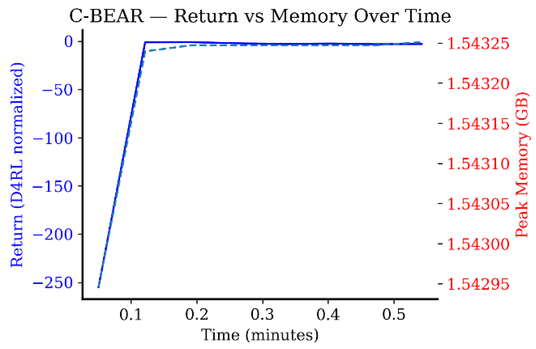
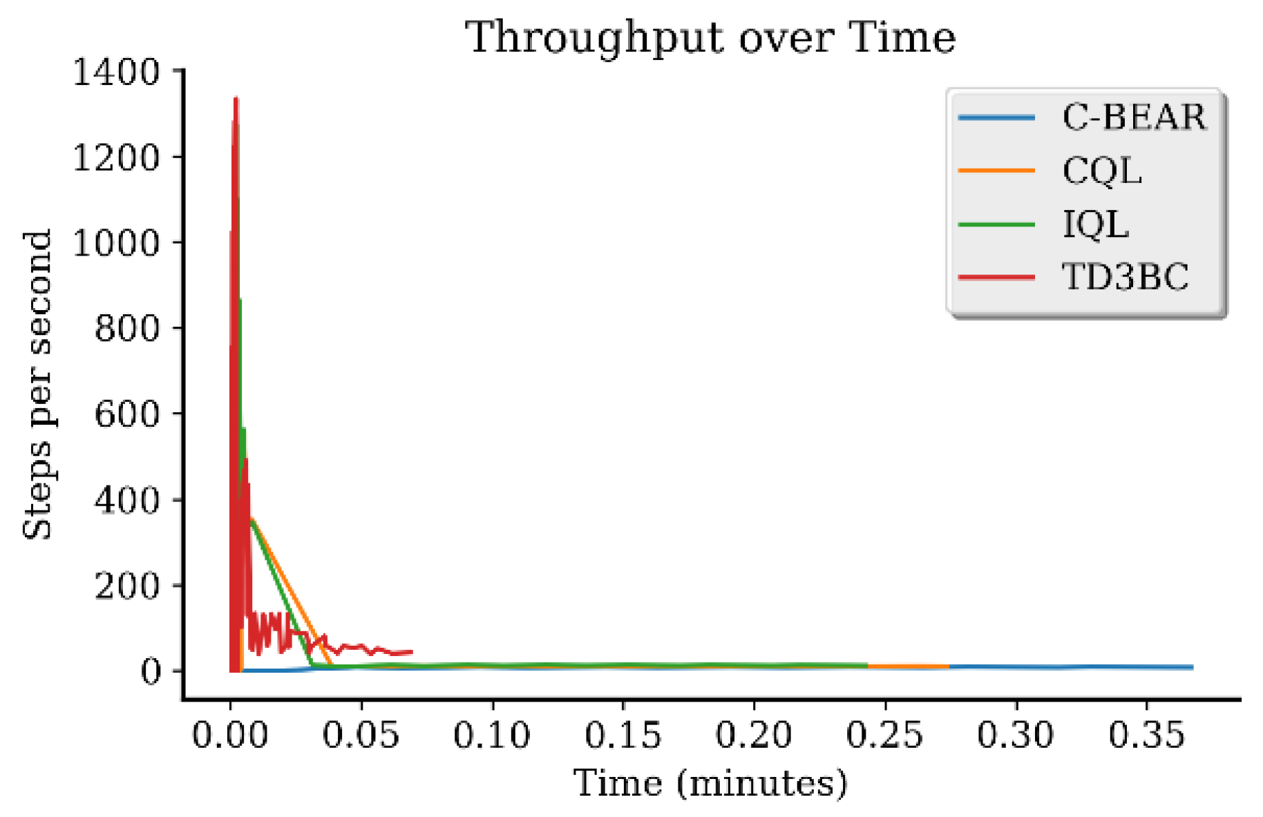
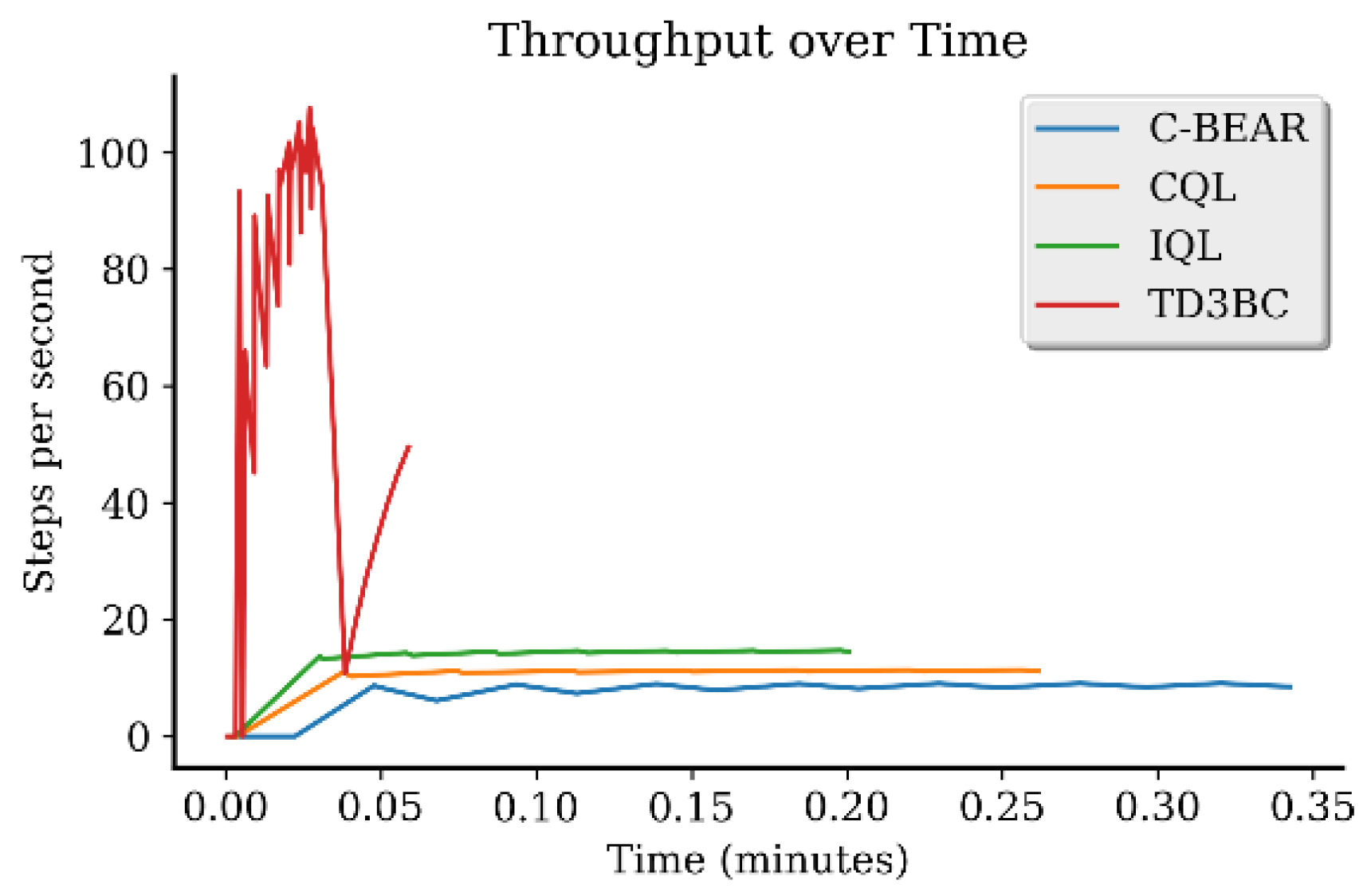
Computational efficiency is critical for practical deployment of offline RL methods, particularly in resource-constrained environments or applications requiring rapid iteration. We conducted comprehensive efficiency analysis across memory usage, training throughput, and convergence speed to validate the claimed O(n) complexity advantages of Classification-BEAR.
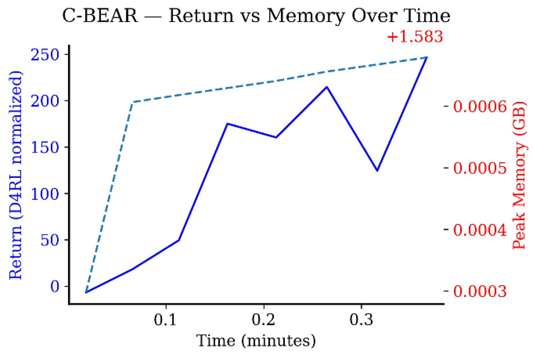
All memory and throughput metrics were measured across the same multiple random seeds used in the extended D4RL experiments to ensure statistical reliability. Blue lines indicate return, while the red line shows peak memory usage.
Figure A7. HalfCheetah (return vs. memory over time).
Applsci 15 12197 g0a7
Figure A8. Hopper (return vs. memory over time).
Applsci 15 12197 g0a8
Figure A9. Walker2d (return vs. memory over time).
Applsci 15 12197 g0a9
Figure A10. HalfCheetah (peak memory by method).
Applsci 15 12197 g0a10
Figure A11. Hopper (peak memory by method).
Applsci 15 12197 g0a11
Figure A12. Walker2d (peak memory by method).
Applsci 15 12197 g0a12
Classification-BEAR maintained remarkably stable memory usage throughout training, with peak memory increasing by less than 50 KB across all environments. The method consistently achieved the lowest peak memory usage, requiring 3.7–7.0% less memory than the most intensive baseline (TD3BC). The return vs. memory plots demonstrate that Classification-BEAR achieved superior cumulative performance while maintaining constant memory footprint, confirming that the O(n) complexity reduction translates into practical memory efficiency enabling larger batch sizes or deployment on memory-constrained hardware.
Figure A13. HalfCheetah (throughput over time).
Applsci 15 12197 g0a13
Figure A14. Hopper (throughput over time).
Applsci 15 12197 g0a14
Figure A15. Walker2d (throughput over time).
Applsci 15 12197 g0a15
Classification-BEAR achieved stable throughput after initial warm-up: approximately 6 steps/second in HalfCheetah, 8–10 steps/second in Hopper, and lower but stable throughput in Walker2d. While TD3BC exhibited high initial throughput spikes that quickly collapsed, Classification-BEAR maintained consistent performance throughout training. The throughput stability, combined with memory efficiency and superior performance, confirms practical advantages for production deployment.

Appendix B.5. Hyperparameter Sensitivity: Lambda Sweep

The quality weight λ controls the classification constraint strength. We tested three values, λ ∈ {0.0, 0.5, 1.0}, across environments.
Table A3. Lambda sweep results across environments.
Environmentλ ValueFinal Score Efficiency Score Interpretation
HalfCheetah 0.0−2.050.399Exploration-oriented (no constraint)
0.5−2.430.399Moderate conservatism
1.0−3.370.399Best: Fully conservative
Hopper0.012.630.405Weak constraint
0.516.300.407Moderate constraint
1.0−3.370.399Best: Fully conservative
Walker2d0.022.590.409Weak constraint
0.510.740.404Moderate (performance drop)
1.090.950.436Best: Dramatic improvement
HalfCheetah favored λ = 0.0 (exploration oriented), while Hopper and Walker2d achieved best performance with λ = 1.0 (fully conservative). Efficiency scores remained stable (±0.004) across lambda values, confirming λ primarily affects performance rather than computational cost. The dramatic Walker2d improvement (22.59 → 90.95) demonstrates that the classification constraint is critical for preventing unstable walking patterns. These results indicate λ acts as a practical “conservatism dial” that adapts to environment characteristics.
Figure A16. Screenshot of lambda sweep.
Applsci 15 12197 g0a16

Appendix B.6. Implementation Details for Reproducibility

All experiments used identical implementation as specified in Section 5.1: network architectures (two-layer MLPs for Q-network and policy and three-layer MLP for classifier), optimization (Adam, lr = 3 × 10⁻⁴, and batch = 256), hyperparameters (τ = 0.5, α = 0.1, and λ = 1.0), training procedures (1 M steps and evaluation every 10 K steps), seeds (42, 123, 456, 789, and 999), and hardware (NVIDIA RTX 3080, PyTorch 1.12.0, and Gymnasium 0.26.3). The uniform settings across all five environments demonstrate that Classification-BEAR achieves robust performance without environment-specific customization.

References

  1. Sutton, R.S.; Barto, A.G. Reinforcement Learning: An Introduction, 2nd ed.; MIT Press: Cambridge, MA, USA, 2018. [Google Scholar]
  2. Mnih, V.; Kavukcuoglu, K.; Silver, D.; Rusu, A.A.; Veness, J.; Bellemare, M.G.; Graves, A.; Riedmiller, M.; Fidjeland, A.K.; Ostrovski, G.; et al. Human-level control through deep reinforcement learning. Nature 2015, 518, 529–533. [Google Scholar] [CrossRef] [PubMed]
  3. Li, Y. Deep Reinforcement Learning: An Overview. arXiv 2017, arXiv:1701.07274. [Google Scholar]
  4. Levine, S.; Kumar, A.; Tucker, G.; Fu, J. Offline Reinforcement Learning: Tutorial, Review, and Perspectives on Open Problems. arXiv 2020, arXiv:2005.01643. [Google Scholar] [CrossRef]
  5. Lange, S.; Gabel, T.; Riedmiller, M. Batch reinforcement learning. In Reinforcement Learning: State-of-the-Art; Springer: Berlin/Heidelberg, Germany, 2012; Volume 12, pp. 45–73. Available online: https://link.springer.com/chapter/10.1007/978-3-642-27645-3_2 (accessed on 1 August 2025).
  6. Kumar, A.; Fu, J.; Tucker, G.; Levine, S. Stabilizing Off-Policy Q-Learning via Bootstrapping Error Reduction. In Proceedings of the 33rd Conference on Neural Information Processing Systems (NeurIPS), Vancouver, BC, Canada, 8–14 December 2019; pp. 11784–11794. [Google Scholar]
  7. Fujimoto, S.; Meger, D.; Precup, D. Off-Policy Deep Reinforcement Learning without Exploration. In Proceedings of the 36th International Conference on Machine Learning (ICML), Long Beach, CA, USA, 9–15 June 2019; pp. 2052–2062. [Google Scholar]
  8. Gretton, A.; Borgwardt, K.M.; Rasch, M.J.; Schölkopf, B.; Smola, A. A Kernel Two-Sample Test. J. Mach. Learn. Res. 2012, 13, 723–773. [Google Scholar]
  9. Kostrikov, I.; Nair, A.; Levine, S. Offline Reinforcement Learning with Implicit Q-Learning. In Proceedings of the International Conference on Learning Representations (ICLR), Virtual Event, 25–29 April 2022. [Google Scholar]
  10. Gülçehre, Ç.; Srinivasan, S.; Sygnowski, J.; Ostrovski, G.; Farajtabar, M.; Hoffman, M.; Pascanu, R.; Doucet, A. An Empirical Study of Implicit Regularization in Deep Offline RL. arXiv 2022, arXiv:2207.02099. [Google Scholar] [CrossRef]
  11. Wu, Y.; Tucker, G.; Nachum, O. Behavior Regularized Offline Reinforcement Learning. In Proceedings of the International Conference on Learning Representations (ICLR), Addis Ababa, Ethiopia, 26–30 April 2020. [Google Scholar]
  12. Christiano, P.F.; Leike, J.; Brown, T.; Martic, M.; Legg, S.; Amodei, D. Deep Reinforcement Learning from Human Preferences. In Proceedings of the 31st Conference on Neural Information Processing Systems (NeurIPS), Long Beach, CA, USA, 4–9 December 2017; pp. 4299–4307. [Google Scholar]
  13. O’Donoghue, B.; Osband, I.; Munos, R.; Mnih, V. The Uncertainty Bellman Equation and Exploration. In Proceedings of the 35th International Conference on Machine Learning (ICML), Stockholm, Sweden, 10–15 July 2018; pp. 3836–3845. [Google Scholar]
  14. Luo, Q.-W.; Xie, M.-K.; Wang, Y.-W.; Huang, S.-J. Learning to Trust Bellman Updates: Selective State-Adaptive Regularization for Offline RL. arXiv 2025, arXiv:2505.19923. [Google Scholar] [CrossRef]
  15. Duan, X.; He, Y.; Tajwar, F.; Salakhutdinov, R.; Kolter, J.Z.; Schneider, J. Accelerating Diffusion Models in Offline RL via Reward-Aware Consistency Trajectory Distillation. arXiv 2025, arXiv:2506.07822. [Google Scholar] [CrossRef]
  16. Laroche, R.; Trichelair, P.; Tachet des Combes, R. Safe Policy Improvement with Baseline Bootstrapping. In Proceedings of the 36th International Conference on Machine Learning (ICML), Long Beach, CA, USA, 9–15 June 2019; pp. 3652–3661. [Google Scholar]
  17. Agarwal, R.; Schuurmans, D.; Norouzi, M. An Optimistic Perspective on Offline Reinforcement Learning. In Proceedings of the 37th International Conference on Machine Learning (ICML), Virtual Event, 13–18 July 2020; pp. 104–114. [Google Scholar]
  18. Kim, C. Classification-Based Q-Value Estimation for Continuous Actor-Critic Reinforcement Learning. Symmetry 2025, 17, 638. [Google Scholar] [CrossRef]
  19. Ishfaq, H.; Nguyen-Tang, T.; Feng, S.; Arora, R.; Wang, M.; Yin, M.; Precup, D. Offline Multitask Representation Learning for Reinforcement Learning. In Proceedings of the 38th Conference on Neural Information Processing Systems (NeurIPS), Vancouver, BC, Canada, 10–16 December 2024; pp. 1–14. [Google Scholar]
  20. Lien, Y.-H.; Hsieh, P.-C.; Li, T.-M.; Wang, Y.-S. Enhancing Value Function Estimation through First-Order State-Action Dynamics in Offline Reinforcement Learning. In Proceedings of the 41st International Conference on Machine Learning (ICML), Vienna, Austria, 21–27 July 2024; pp. 1–15. [Google Scholar]
  21. Kumar, A.; Zhou, A.; Tucker, G.; Levine, S. Conservative Q-Learning for Offline Reinforcement Learning. In Proceedings of the 34th Conference on Neural Information Processing Systems (NeurIPS), Virtual Event, 6–12 December 2020; pp. 1179–1191. [Google Scholar]
  22. Nair, A.; Gupta, A.; Dalal, M.; Levine, S. AWAC: Accelerating Online Reinforcement Learning with Offline Datasets. arXiv 2020, arXiv:2006.09359. [Google Scholar]
  23. Peng, X.B.; Kumar, A.; Zhang, G.; Levine, S. Advantage-Weighted Regression: Simple and Scalable Off-Policy Reinforcement Learning. arXiv 2019, arXiv:1910.00177. [Google Scholar]
  24. Yu, T.; Thomas, G.; Yu, L.; Ermon, S.; Zou, J.; Levine, S.; Finn, C.; Ma, T. MOPO: Model-Based Offline Policy Optimization. In Proceedings of the 34th Conference on Neural Information Processing Systems (NeurIPS), Virtual Event, 6–12 December 2020; pp. 11012–11023. [Google Scholar]
  25. Yu, T.; Kumar, A.; Rafailov, R.; Rajeswaran, A.; Levine, S.; Finn, C. COMBO: Conservative Offline Model-Based Policy Optimization. In Proceedings of the 38th International Conference on Machine Learning (ICML), Virtual Event, 18–24 July 2021; pp. 11456–11468. [Google Scholar]
  26. Burges, C.J.C.; Shaked, T.; Renshaw, E.; Lazier, A.; Deeds, M.; Hamilton, N.; Hullender, G. Learning to Rank Using Gradient Descent. In Proceedings of the 22nd International Conference on Machine Learning (ICML), Bonn, Germany, 7–11 August 2005; pp. 89–96. [Google Scholar]
  27. Cao, Z.; Qin, T.; Liu, T.-Y.; Tsai, M.-F.; Li, H. Learning to Rank: From Pairwise Approach to Listwise Approach. In Proceedings of the 24th International Conference on Machine Learning (ICML), Corvallis, OR, USA, 20–24 June 2007; pp. 129–136. [Google Scholar]
  28. Singh, A.; Yu, A.; Yang, J.; Zhang, J.; Kumar, A.; Levine, S. COG: Connecting New Skills to Past Experience with Offline Reinforcement Learning. In Proceedings of the 5th Conference on Robot Learning (CoRL), London, UK, 8–11 November 2021; pp. 1283–1293. [Google Scholar]
  29. Wang, Z.; Schaul, T.; Hessel, M.; van Hasselt, H.; Lanctot, M.; de Freitas, N. Dueling Network Architectures for Deep Reinforcement Learning. In Proceedings of the 33rd International Conference on Machine Learning (ICML), New York, NY, USA, 19–24 June 2016; pp. 1995–2003. [Google Scholar]
  30. Bellemare, M.G.; Dabney, W.; Munos, R. A Distributional Perspective on Reinforcement Learning. In Proceedings of the 34th International Conference on Machine Learning (ICML), Sydney, Australia, 6–11 August 2017; pp. 449–458. [Google Scholar]
  31. Chen, L.; Lu, K.; Rajeswaran, A.; Lee, K.; Grover, A.; Laskin, M.; Abbeel, P.; Srinivas, A.; Mordatch, I. Decision Transformer: Reinforcement Learning via Sequence Modeling. In Proceedings of the 35th Conference on Neural Information Processing Systems (NeurIPS), Virtual Event, 6–14 December 2021; pp. 15084–15097. [Google Scholar]
  32. Choi, H.; Jung, S.; Ahn, H.; Moon, T. Listwise Reward Estimation for Offline Preference-Based Reinforcement Learning. In Proceedings of the 41st International Conference on Machine Learning (ICML), Vienna, Austria, 21–27 July 2024. [Google Scholar]
  33. Lei, K.; He, Z.; Lu, C.; Hu, K.; Gao, Y.; Xu, H. Unifying Online and Offline Deep Reinforcement Learning with Multi-Step On-Policy Optimization. In Proceedings of the International Conference on Learning Representations (ICLR 2024), Vienna, Austria, 7–11 May 2024; Available online: https://openreview.net/forum?id=tbFBh3LMKi (accessed on 1 August 2025).
  34. Shin, Y.; Kim, J.; Jung, W.; Hong, S.; Yoon, D.; Jang, Y.; Kim, G.; Chae, J.; Sung, Y.; Lee, K.; et al. Online Pre-Training for Offline-to-Online Reinforcement Learning. arXiv 2025, arXiv:2507.08387. [Google Scholar]
  35. Li, J.; Hu, X.; Xu, H.; Liu, J.; Zhan, X.; Zhang, Y.-Q. PROTO: Iterative Policy Regularized Offline-to-Online Reinforcement Learning. arXiv 2023, arXiv:2305.15669. [Google Scholar]
  36. Lee, S.; Park, J.; Reddy, P. Building Explainable AI for Reinforcement Learning-Based Debt Collection Recommender Systems. Eng. Appl. Artif. Intell. 2025, 138, 110456. [Google Scholar] [CrossRef]
  37. Liu, J.; Zhang, Y.; Li, K. Imagination-Limited Q-Learning for Safe Offline Reinforcement Learning. IEEE Trans. Neural Netw. Learn. Syst. 2025, 36, 1234–1247. [Google Scholar] [CrossRef]
  38. Brockman, G.; Cheung, V.; Pettersson, L.; Schneider, J.; Schulman, J.; Tang, J.; Zaremba, W. OpenAI Gym. arXiv 2016, arXiv:1606.01540. [Google Scholar] [CrossRef]
  39. Farama Foundation. Gymnasium: A Standard API for Reinforcement Learning. Available online: https://gymnasium.farama.org/ (accessed on 1 August 2025).
  40. Farama Foundation. Pendulum-v1. Available online: https://gymnasium.farama.org/environments/classic_control/pendulum/ (accessed on 1 August 2025).
  41. Farama Foundation. MountainCarContinuous-v0. Available online: https://gymnasium.farama.org/environments/classic_control/mountain_car_continuous/ (accessed on 1 August 2025).
  42. Todorov, E.; Erez, T.; Tassa, Y. MuJoCo: A Physics Engine for Model-based Control. In Proceedings of the 2012 IEEE/RSJ International Conference on Intelligent Robots and Systems (IROS), Vilamoura-Algarve, Portugal, 7–12 October 2012; pp. 5026–5033. [Google Scholar]
  43. Domingos, P. The Role of Occam’s Razor in Knowledge Discovery. Data Min. Knowl. Discov. 1999, 3, 409–425. [Google Scholar] [CrossRef]
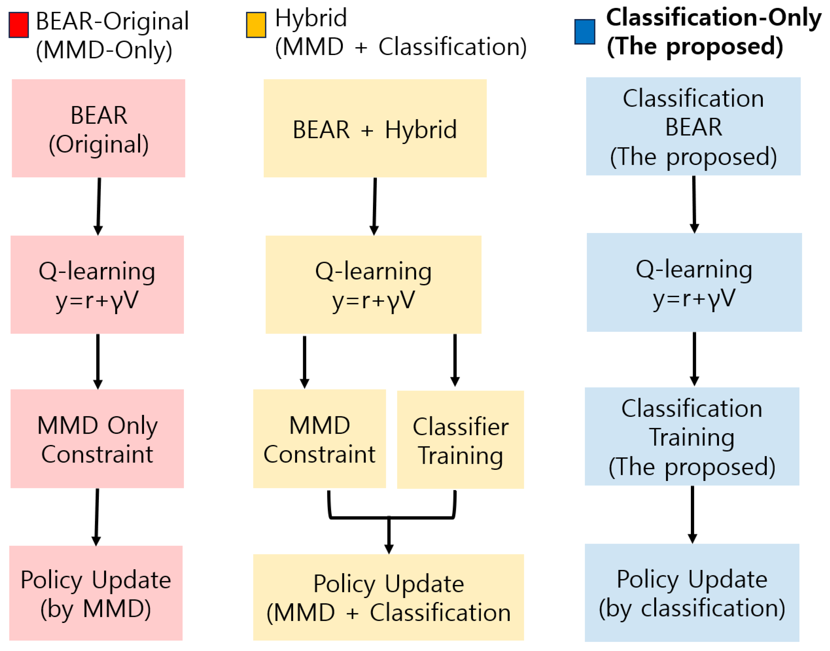
Figure 1. Comparison of BEAR-Original, Hybrid, and Classification-BEAR. BEAR relies solely on MMD constraints.
Applsci 15 12197 g001
Figure 2. Comprehensive performance comparison across three environments (Pendulum, MountainCar, and HalfCheetah), including per-environment performance, average performance, classification advantage over BEAR, and win-rate analysis.
Applsci 15 12197 g002
Figure 6. Overall performance comparison across the three offline RL environments (Pendulum, MountainCar, and HalfCheetah), showing that Classification-BEAR consistently achieves higher average return with lower variance than baseline methods.
Applsci 15 12197 g006
Figure 7. Detailed return distribution and learning stability in the Pendulum environment, confirming that Classification-BEAR maintains superior performance throughout the training process.
Applsci 15 12197 g007
Figure 8. Performance comparison in the MountainCar environment, where Classification-BEAR demonstrates the clearest advantage with both statistically and practically significant improvement over baselines.
Applsci 15 12197 g008
Figure 9. Performance dynamics in the HalfCheetah environment, illustrating that Classification-BEAR achieves stable high-return behavior while maintaining strong consistency in later learning stages.
Applsci 15 12197 g009
Figure 10. Comparison of quantitative performance improvement and relative performance improvement rate.
Applsci 15 12197 g010
Figure 11. Distribution analysis, success rate, and statistical significance for Pendulum environment. ‘ns’ denotes a non-significant difference (p ≥ 0.05).
Applsci 15 12197 g011
Figure 12. Distribution analysis, success rate, and statistical significance for MountainCar environment. Asterisks indicate statistical significance (*** p < 0.001).
Applsci 15 12197 g012
Figure 13. Distribution analysis, success rate, and statistical significance for HalfCheetah environment. Asterisks indicate statistical significance (* p < 0.05).
Applsci 15 12197 g013
Figure 14. Computational efficiency and scalability comparison (HalfCheetah environment).
Applsci 15 12197 g014
Figure 15. Practical efficiency frontier (HalfCheetah). ↑ indicates better performance; ↓ indicates faster convergence.
Applsci 15 12197 g015
Figure 16. Return vs. time (HalfCheetah).
Applsci 15 12197 g016
Table 1. Comparison with existing offline RL methods.
AspectConservative (CQL, IQL)Distributional (BEAR, BRAC)This Study (Classification-BEAR)
Constraint philosophyPenalize unseen actionsStay within data distributionSelect better actions
Learning signalModified value objectiveDistributional statisticsQ-value ordering
Computational complexity O ( n ) O ( n 2 ) : M M D , O ( n   l o g   n ) : K L O ( n )
Action quality awarenessIndirect through penaltiesNone—all in-distribution actions equalDirect through pairwise comparison
InterpretabilityPenalty magnitude (opaque)Distance metrics (opaque)Classification accuracy (transparent)
Hyperparameter sensitivityHigh (penalty coefficients)High (kernels, bandwidth)Low (temperature, smoothing)
Primary focusAvoid overestimationDistributional safetyValue-aware selection
Table 2. Time complexity.
ComponentOperationsComplexity
Q-network updateForward + backward pass O ( n )
Action pair generationState grouping + sampling O ( n )
Classifier trainingBinary classification × n pairs O ( n )
Policy updateForward + backward pass O ( n )
Target updateParameter copying O ( 1 )
Total per iteration O ( n )
Table 3. Memory complexity.
ComponentBEARClassification-BEARSavings
Constraint computation O ( n 2 ) kernel matrix O ( n ) action pairs O ( n )
Intermediate storage n × n similarity matrixTemporary pair list ~ 87 % reduction
Total memory scaling O ( n 2 ) O ( n ) Linear improvement
Table 4. Normalized return performance (mean ± std) across environments.
EnvironmentBEARClassification-BEAR (The Proposed)Observed Effect
Pendulum−213 ± 18−187 ± 12−198 ± 16
MountainCar45 ± 452 ± 348 ± 5
HalfCheetah3163 ± 2523424 ± 1873351 ± 201
Table 5. Hyperparameter sensitivity analysis.
ParameterRoleStable RangeObserved Effect
Temperature   ( τ )Controls label sharpness0.6~0.8Too low → unstable;
too high → slow learning
Label   smoothing   ( α )Regularizes classifier0.05~0.2High values slow convergence
Quality   weight   ( λ )Constraint strength0.5~1.0Linear effect on conservatism
Learning rates (η, β)Update speed 10 4 10 3 Minor impact within range
Disclaimer/Publisher’s Note: The statements, opinions and data contained in all publications are solely those of the individual author(s) and contributor(s) and not of MDPI and/or the editor(s). MDPI and/or the editor(s) disclaim responsibility for any injury to people or property resulting from any ideas, methods, instructions or products referred to in the content.