Determining the Optimal T-Value for the Temperature Scaling Calibration Method Using the Open-Vocabulary Detection Model YOLO-World

Abstract

Object detection is an important tool in many areas, such as robotics or autonomous driving. Especially in these areas, a wide variety of object classes must be detected or interacted with. Models from the field of Open-Vocabulary Detection (OVD) provide a solution here, as they can detect not only base classes but also novel object classes, i.e., those classes that were not seen during training. However, one problem with OVD models is their poor calibration, meaning that the predictions are often too over- or under-confident. To improve the calibration, Temperature Scaling is used in this study. Using YOLO World, one of the best-performing OVD models, the aim is to determine the optimal T-value for this calibration method. For this reason, it is investigated whether there is a correlation between the logit distribution and the optimal T-value and how this can be modeled. Finally, the influence of Temperature Scaling on the Expected Calibration Error (ECE) and the mAP (Mean Average Precision) will be analyzed. The results of this study show that similar logit distributions of different datasets result in the same optimal T-values. This correlation could be best modeled using Kernel Ridge Regression (KRR) and Support Vector Machine (SVM). In all cases, the ECE could be improved by Temperature Scaling without significantly reducing the mAP.

1. Introduction

Object detection plays an essential role in areas such as robotics and autonomous driving. Without reliable object detection, objects cannot be perceived, nor can interaction with them take place. A major challenge in this context is the detection of unknown object classes, i.e., those classes that the model has not seen during training. Many deep learning (DL) and machine learning (ML) approaches such as YOLO [1] or Faster R-CNN [2] train models on specific object classes and can only detect these during inference. Despite the generally good detection rate, it is not possible to detect object classes outside the training dataset. Adding new classes costs time and resources, as a new dataset must be created for each object class and the model must be retrained.

This limitation has given rise to the field of Open-Vocabulary Detection (OVD) [3], where models are being developed that can also detect object classes outside the training dataset. A model is therefore trained using base classes and can detect novel classes as well. There are currently a large number of Open-Vocabulary Detection models, such as mm-Grounding DINO [4], Det-CLIPv3 [5], Grounding DINO [6], Grounding DINO 1.5 Pro [7] and YOLO-World [8], to name a few methods. All these models have different structures and approaches to detecting unknown objects.

Grounding DINO and mm-Grounding DINO use a Swin Transformer [9] backbone to extract image features and a BERT [10] backbone to extract text features. In comparison, YOLO-World relies on a lightweight YOLOv8 backbone to extract image features, which greatly improves the inference speed compared to Grounding DINO and mm-Grounding DINO. In addition, CLIP [11] text encoder is used instead of BERT. DetCLIPv3 also trains a Swin-T and Swin-L backbone. One problem with the use and comparison of these models is the open-source access and the pre-training datasets. For example, the source code of DetCLIPv3 is not publicly available, just like that of Grounding DINO 1.5 Pro. For this reason, modifications to the source code, as required for this study, are not possible. Furthermore, Grounding DINO 1.5 Pro uses its own pre-training dataset (Grounding-20M), which is also not publicly available. This makes it nearly impossible to compare it with other models, such as YOLO-World, especially with regard to the detection of unknown objects under OVD conditions.

However, when comparing open-source models that use the same or similar pre-training datasets in terms of the accuracy of their predictions under OVD conditions, YOLO-World and mm-Grounding DINO currently prove to be the best performing models. Accuracy is assessed using the mAP (mean average precision) and LVIS minival [12] (a subset of LVIS [13]) is used as the evaluation dataset. mm-Grounding DINO was pre-trained using the Ojects365v1 [14] and GoldG [12] datasets, while YOLO-World-V2.1 also includes CC-LiteV2 [15] in addition to Ojects365v1 and GoldG. The achieved mAP is 35.7% for mm-Grounding DINO [4] and 35.5% for YOLO-World-V2.1-L [15]. However, in terms of inference speed, YOLO-World is significantly faster at around 52.0 FPS on one NVIDIA V100 GPU, while Grounding DINO only achieves 1.5 FPS [8] (mm-Grounding DINO is based almost unchanged on the Grounding DINO model [4], hence the inference speeds are in the same order of magnitude). Therefore, the investigations in this study focus on the open-source model YOLO-World-V2.1.

In addition to accuracy and inference speed, the calibration of these models is also essential for the use of OVD models in the real world. It was demonstrated in [16] that YOLO-World is not well calibrated; the model is overconfident in its predictions. If many false positive (FP) predictions occur with a high confidence value, this suggests a trustworthy prediction, even though the object being searched for was not correctly detected. Many such predictions can result in personal injury and property damage, especially in safety-critical applications. It is therefore important that OVD models are well calibrated. There are numerous methods for correcting miss-calibration, which are listed in [17,18] for neural networks. In [19], the simple calibration method Temperature Scaling is applied to CLIP to reduce the calibration error. The study [16] showed that Temperature Scaling can positively influence the calibration of the OVD model YOLO-World by reducing the calibration error. However, the optimal T-value depends heavily on the calibration dataset used, i.e., a suitable calibration dataset was able to reduce the Expected Calibration Error (ECE) by several percent, while an unsuitable dataset resulted in a suboptimal T-value and increased the ECE.

The objectives of this study can be derived from the findings in [16]. Since the calibration dataset has a decisive influence on the determination of the optimal T-value, the first step is to investigate whether there is a correlation between different datasets and the optimal T-values of the Temperature Scaling calibration method. To this end, the logit distributions according to the YOLO-World prediction of a dataset will be analyzed. The optimal T-values will be determined with a view to minimizing the ECE. Subsequently, the extent to which the optimal T-values can be predicted from a given logit distribution will be investigated. Various machine learning models will be tested to model the relationship. Finally, the accuracy (mAP) will be examined once after calibration, i.e., after optimization of the ECE, as the mAP should not decrease significantly despite improved calibration. In addition, the influence of temperature scaling on the ECE of the respective datasets is also analyzed.

The results of this investigation show that there is a correlation between the logit distribution and the optimal T-values, i.e., if two distributions are similar, they also result in the same optimal T-values. Different distributions have T-values that differ from each other. This makes it possible to predict the optimal T-values based on a given logit distribution. After calibration using temperature scaling, the mAP decreases slightly or remains unchanged when the T-value is less than 1 and increases in most cases when T is greater than 1. An improvement in ECE was achieved in all cases.

2. Related Work

2.1. YOLO-World

YOLO-World is a powerful object detection model with real-time Open-Vocabulary detection capabilities [8]. As input, YOLO-World receives an image I and a text F, from which the text embeddings $W=TextEncoder\left(F\right)\in {\mathbb{R}}^{C\times D}$ and the object embeddings ${\left\{e_k\right\}}_{k=1}^K$ ($e_k\in {\mathbb{R}}^D$) are derived. D reflects the embedding dimension, C is the number of classes and K is the number of objects. A frozen CLIP text encoder is used to extract the text embeddings. The image features are extracted by a YOLOv8 backbone, which are converted into object embeddings using the RepVL-PAN (Re-parameterizable Vision-Language Path Aggregation Network) and the text contrastive head. Subsequently, the text embeddings are L2-normalized (L2-Norm), while the object embeddings are batch-normalized (Batch-Norm) [15]. The logits (object-text similarity) $l_{k,j}$ between the j-th text embedding $w_j\in W$ and the k-th object embedding $e_k$ can be calculated by

$$l_{k,j}=\alpha ·\mathrm{Batch-Norm}\left(e_k\right)·\mathrm{L2-Norm}{\left(w_j\right)}^T+\beta .$$

(1)

$\alpha$ and $\beta$ are two constants, which scale and shift the result. Detailed explanations of how YOLO-World works are provided in [8]. Finally, the logits are activated by a sigmoid function,

$$\sigma \left(l_{k,j}\right)={\displaystyle \frac{1}{1+e^{-l_{k,j}}}},$$

(2)

which then yields the corresponding probabilities or confidence values of the predictions. Unlike a softmax activation function, all logits are considered independently of each other.

2.2. Temperature Scaling

Temperature scaling is a method designed to improve the calibration of a model. It scales the logits of a model using a constant value, the temperature value $T>0$ [17,18]. Temperature scaling can therefore be applied after a model has been trained and has proven to be a simple but efficient method in the literature [18]. This method is applied before the logits are activated by a softmax function, but can also be applied to other activation functions, such as sigmoid. The logits after calibration $l_{k,j}^{cal}$ can be calculated as

$$l_{k,j}^{cal}={\displaystyle \frac{l_{k,j}}{T}}.$$

(3)

where $l_{k,j}$ represents the logits before calibration. Usually, a calibration dataset is required to determine the optimal T-value.

2.3. Expected Calibration Error

A commonly used metric for quantitatively determining the calibration error is the expected calibration error (ECE) [17,18].

After a prediction, a sample i consists of a confidence value ${\widehat{p}}_i$, a predicted class label ${\widehat{y}}_i$, a predicted bounding box ${\widehat{b}}_i$, a true class label $y_i$ and a true bounding box $b_i$. Based on this information, a sample can be categorized as either a true positive ($t_i=1$) or a false positive ($t_i=0$). A detailed description of how to determine a true positive and a false positive can be found in [16]. According to the confidence values ${\widehat{p}}_i$, all samples i can be divided into M equally sized bins $B_1,\dots ,B_M$, where the bin $B_m$ ($m\in \{1,\dots ,M\}$) includes all samples of the interval $I_m=({\displaystyle \frac{m-1}{M}},{\displaystyle \frac{m}{M}}]$. The interval size is fixed and is $1/M$.

To determine the ECE, the accuracy $acc\left(B_m\right)$ and confidence $conf\left(B_m\right)$ must be calculated for each bin $B_m$. The accuracy $acc\left(B_m\right)$ represents the ratio of true positives to the total number of samples ($|B_m|$) of the bin $B_m$ and can be calculated using the equation

$$acc\left(B_m\right)={\displaystyle \frac{1}{|B_m|}}\sum _{i\in B_m}{t}_i.$$

(4)

The confidence $conf\left(B_m\right)$ is the average of all confidence values ${\widehat{p}}_i$ that are in Bin $B_m$ and is defined as

$$conf\left(B_m\right)={\displaystyle \frac{1}{|B_m|}}\sum _{i\in B_m}{\widehat{p}}_i.$$

(5)

Finally, the expected calibration error can be derived based on the accuracy and confidence. The ECE is the weighted average of the difference between $acc\left(B_m\right)$ and $conf\left(B_m\right)$ across all bins $B_m$,

$$ECE=\sum _{m=1}^M{\displaystyle \frac{|B_m|}{n}}|acc\left(B_m\right)-conf\left(B_m\right)|,$$

(6)

where n is the total number of all samples i. The ECE is equal to 0 for a perfectly calibrated model, i.e., $acc\left(B_m\right)=conf\left(B_m\right)$ for all bins $B_1,\dots ,B_M$.

2.4. Limitations of Existing Methods

In comparison to other methods for determining the optimal T-value, such as cross-validation [20,21], one of the practical advantages of the proposed approach lies in the reduced time required. Once test data has been collected and an ML model has been trained, the optimal T-value can be easily predicted using a practically obtained logit distribution, without having to test numerous possibilities. The biggest advantage of the proposed approach is its real-world applicability, as no ground truth annotations/labelings need to be created from the collected object detection data (e.g., from a robot) in order to determine an optimal T-value. Cross-validation cannot be used in this case.

In addition, temperature scaling was preferred over more powerful methods such as vector scaling and matrix scaling [18], as only one optimal value needs to be determined, which is much easier to achieve with little data (logit distributions) when a post-hoc calibration improvement is the objective. In contrast, vector scaling and matrix scaling require a large number of values to be optimized, which means that more training data is needed, which is difficult to generate. Furthermore, the computational effort required to determine the optimal T-values per dataset is higher, as significantly more combinations have to be tested.

3. Methodology

3.1. Overall Approach

This study aims to determine whether there is a correlation between the logit distributions and the optimal T-values of different datasets in order to achieve the best possible calibration using the Temperature Scaling calibration method. Furthermore, the extent to which modeling is possible is investigated, i.e., whether the optimal T-values can be predicted based on a given logit distribution. Finally, the influence of the method on the accuracy (mAP) and calibration error (ECE) of the predictions is determined.

For all investigations carried out within the scope of this study, the model YOLO-World-V2.1-L (resolution: 1280) [15] is used, which detects objects using bounding boxes. A maximum of 300 predictions per image will be accepted (default setting). The reasons for using this model are listed in Section 1. The literature source [16] explains how false positives (FP) and true positives (TP) are determined.

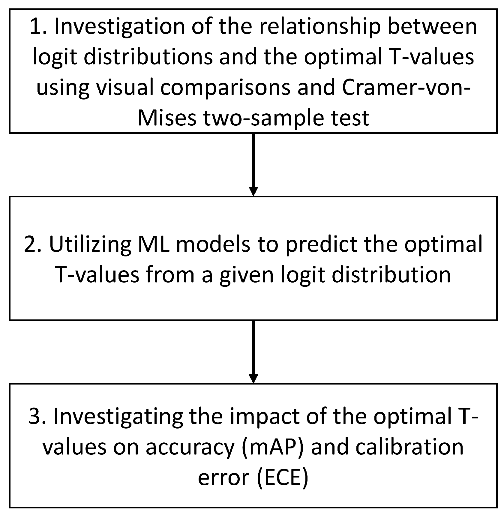
Figure 1 provides a summary of the methodology. In the first step, the relationship between the logit distributions and the optimal T-values is investigated. To do this, the optimal T-values of different datasets must first be determined, which differ from each other depending on the dataset. In total, the optimal T-values are derived from 7 different datasets (LVIS minival [12], Open Images V7 [22,23], Pascal VOC [24], COCO [25], EgoObjects [26], Objects365v1 [14] and a self-created dataset (see Section 3.2)) with different variants (see Section 4.1 for further explanations).

As a metric that should be minimized, the ECE is used, which can be calculated according to Equation (6). This means that a T-value is optimal if the ECE is minimal. Based on [16], two IoU (intersection over union) threshold values ($IoU=0.5$ and $IoU=0.75$) are considered for the calculation of the ECE, i.e., there are also two corresponding optimal T-values, one for the minimum $ECE@[\mathrm{IoU}=0.5]$ and one for the minimum $ECE@[IoU=0.75]$. The temperature values are set to $T\in \{0.4+0.05·u\mid u\in \mathbb{Z},0\le u\le 32\}$ in accordance with [16,19]. The set contains $T=0.4$ as the minimum and $T=2.0$ as the maximum value. For each of these T-values contained in the set, the $ECE@[IoU=0.5]$ and the $ECE@[IoU=0.75]$ are calculated and the minimum is derived. For the calculation of the ECE, $M=10$ applies to all investigations.

After the optimal T-values have been determined for each dataset, the logit distribution is extracted, which contains the logits of all predictions of a dataset, which are then filtered. Since YOLO-World uses an internal confidence threshold of 0.001 for all predictions, i.e., YOLO-World rejects all predictions whose confidence is less than equal to 0.001, it follows from Equations (2) and (3) that

$$0.001<{\displaystyle \frac{1}{1+e^{-l_{k,j}^{cal}}}}=\sigma \left(l_{k,j}^{cal}\right),$$

(7)

and rearranged to $l_{k,j}^{cal}$, this results in

$$l_{k,j}^{cal}>-ln\left({\displaystyle \frac{1-0.001}{0.001}}\right)\approx -6.9068.$$

(8)

This means that only the logit values that satisfy the condition from Equation (8) are retained, which greatly reduces the number of logits, since these would not be considered anyway. The logit distribution is always determined at a T-value of $T=1.0$, which corresponds to the prediction of YOLO-World without temperature scaling.

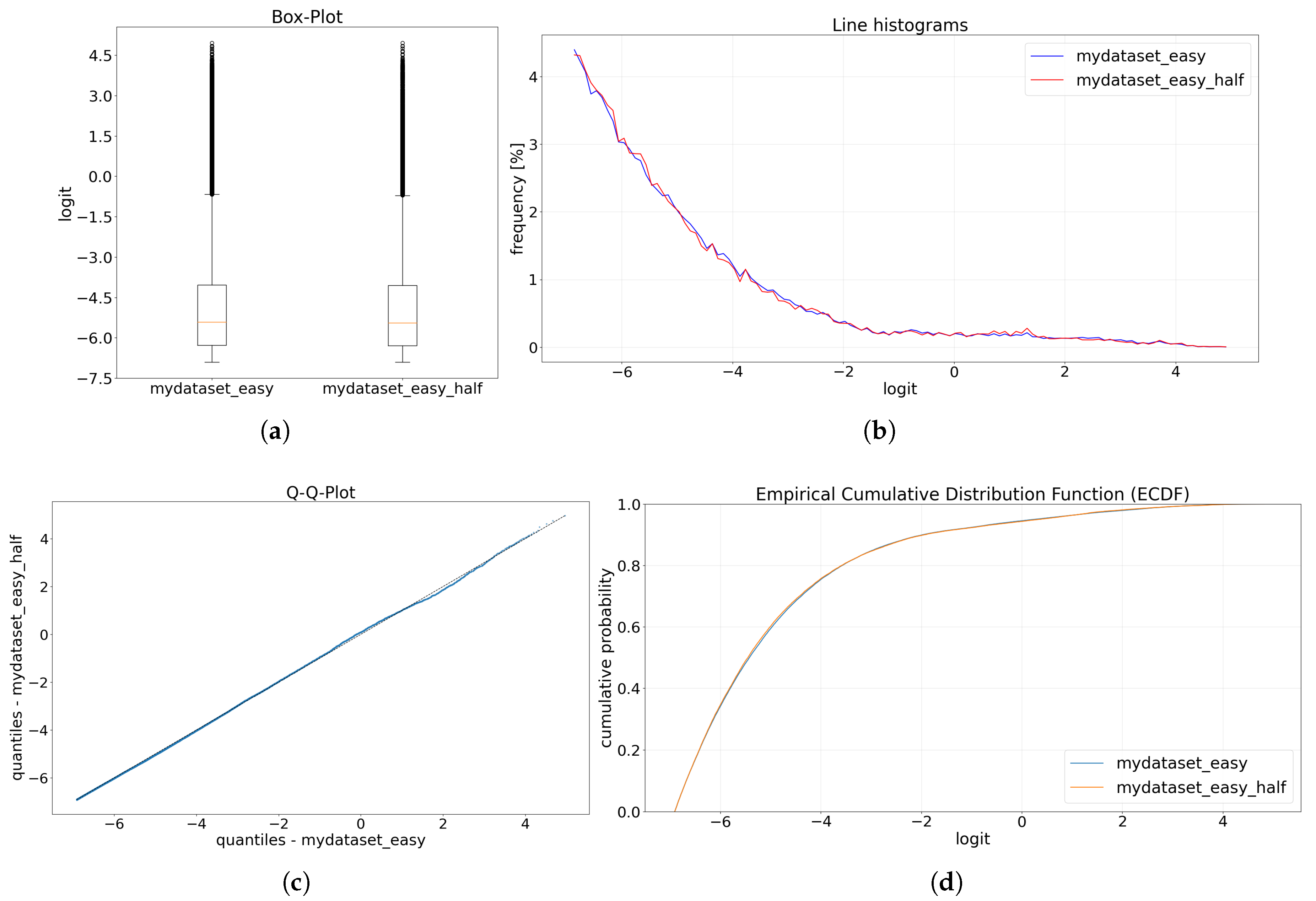
To check the relationship between the optimal T-values and the logit distributions, selected distributions are first tested visually to obtain an initial assessment of whether the same optimal T-values are also based on similar distributions and whether unequal T-values have dissimilar distributions. For the visual comparison, four diagrams are used: box plot, line histogram, Q-Q plot (quantile-quantile plot) and ECDF (empirical cumulative distribution function) plot. The box plot is shown here by default with the first quartile, median and third quartile, where the whiskers according to Tukey [27] can be calculated as 1.5 times the interquartile range (IQR). Outliers (data points outside the whiskers) are marked as points [28]. For the Q-Q plot, a total of 10,000 quantiles are calculated per logit distribution and these are plotted against each other for two distributions. The bin size of the histograms for the division of the logits is calculated using the Freedman-Diaconis Estimator [29], whereby the bin sizes from both logit distributions to be compared are calculated together. A line histogram is then derived from the bin histogram by replacing all bins with a point in the center of the respective bin, which are connected to form a line. In addition, the frequency of the vertical axis is given as a percentage.

After the visual examination, the logit distributions of selected datasets should be compared with each other using a statistical test. This is another way to show that similar distributions result in the same optimal T-values and that different distributions also have different T-values. As a statistical test, the Cramer-von-Mises two-sample test [30] is used for this investigation. The null hypothesis of this test states that two samples come from the same distribution. This is considered to be fulfilled if $p>\eta$, where the standard value $\eta =0.05$ is assumed in this study. In addition to the statistical test, the Earth Mover’s Distance (EMD) [31,32] and the non-parametric effect size Cliff’s Delta [33] are calculated in order to make further conclusions regarding a correlation between the optimal T-values and the logit distributions. If there is an exact match between two logit distributions, both EMD and Cliff’s Delta are 0. So if two distributions have the same optimal T-values, then EMD and Cliff’s Delta should be very small.

After the relationship between the logit distributions and the optimal T-values has been investigated, this relationship is modeled in the second step utilizing machine learning (ML) methods. The general scheme is illustrated in Figure 2. Since the number of logits depends on the number of classes and the number of images, the distributions have different sizes. Furthermore, a logit distribution sometimes consists of several million logits, which means it is not reasonable to use them directly as input for the ML model. Instead, the distribution is mapped using summary statistics, as suggested in [34], which then serve as input for the ML model. As output/prediction, the optimal T-values for an IoU threshold of 0.5 and 0.75 are obtained, which minimize the respective ECE most, i.e., achieve the best calibration.

To quantify the prediction errors, three error metrics Mean Absolute Error (MAE), Root Mean Square Error (RMSE) and coefficient of determination (R²) are calculated, as suggested in [35]. The bootstrap resampling method [36,37] is used to measure the uncertainty of these errors, where S corresponds to the number of bootstrap runs ($s\in \{1,\dots ,S\}$). The error metrics can be interpreted and calculated as follows, based on [35,38]. The MAE indicates the average deviation between the predicted T-values ${\widehat{T}}_{z,\delta }^{\left(s\right)}$ and the true optimal T-values $T_{z,\delta }^{\left(s\right)}$, i.e., it is the average prediction error of the ML models. Here, $Z^{\left(s\right)}$ represents the number of true optimal T-values (or predicted T-values) for each bootstrap run s per IoU threshold $\delta \in \{0.5,0.75\}$. In addition, $z\in \{1,\dots ,Z^{\left(s\right)}\}$ applies. The RMSE is also calculated from the mean of the difference between ${\widehat{T}}_{z,\delta }^{\left(s\right)}$ and $T_{z,\delta }^{\left(s\right)}$, however the difference is squared, which means that large deviations are weighted more heavily. Afterwards, the square root is taken from the result. With the help of R², it is possible to describe how well the model can explain the variance of the dependent variable ($T_{z,\delta }^{\left(s\right)}$) based on the input data (summary statistics of the logit distribution) in comparison to the mean ${\overline{T}}_{\delta }^{\left(s\right)}$. In general, the smaller the MAE and the RMSE are, the better the prediction of the model is, while an R² value approaching 1 means that the variance could be explained perfectly. The MAE, RMSE, and R² can be calculated as a function of the IoU thresholds $\delta$ and of the bootstrap run s as follows:

$${MAE}^{\left(s\right)}@[IoU=\delta ]={\displaystyle \frac{1}{Z^{\left(s\right)}}}\sum _{z=1}^{Z^{\left(s\right)}}\left|{\widehat{T}}_{z,\delta }^{\left(s\right)}-T_{z,\delta }^{\left(s\right)}\right|,$$

(9)

$${RMSE}^{\left(s\right)}@[IoU=\delta ]=\sqrt{{\displaystyle \frac{1}{Z^{\left(s\right)}}}\sum _{z=1}^{Z^{\left(s\right)}}{\left({\widehat{T}}_{z,\delta }^{\left(s\right)}-T_{z,\delta }^{\left(s\right)}\right)}^2},$$

(10)

$$R^{2,\left(s\right)}@[IoU=\delta ]=1-{\displaystyle \frac{{\sum }_{z=1}^{Z^{\left(s\right)}}{\left({\widehat{T}}_{z,\delta }^{\left(s\right)}-T_{z,\delta }^{\left(s\right)}\right)}^2}{{\sum }_{z=1}^{Z^{\left(s\right)}}{\left(T_{z,\delta }^{\left(s\right)}-{\overline{T}}_{\delta }^{\left(s\right)}\right)}^2}},$$

(11)

where,

$${\overline{T}}_{\delta }^{\left(s\right)}={\displaystyle \frac{1}{Z^{\left(s\right)}}}\sum _{z=1}^{Z^{\left(s\right)}}{T}_{z,\delta }^{\left(s\right)}.$$

(12)

In addition, all predicted T-values ${\widehat{T}}_{z,\delta }^{\left(s\right)}$ are rounded to the next multiple of 0.05 before the errors are calculated, since the true T-values $T_{z,\delta }^{\left(s\right)}$ are also only available in intervals of 0.05. Subsequently, the median and the 95% percentile bootstrap confidence intervals [39] are determined from the S bootstrap runs of the 3 error metrics. Therefore, the errors $MAE@[IoU=\delta ]$, $RMSE@[IoU=\delta ]$ and $R^2@[IoU=\delta ]$ are always given as the median and 95% confidence interval ($[Q0.025,Q0.975]$).

In the third and final step, a discussion of the calibration error (ECE) and the accuracy (mAP) should take place. On the one hand, it should be investigated how much the ECE could be improved by the temperature scaling calibration procedure, based on the respective datasets. In this way, the efficiency of this procedure should be derived. On the other hand, the mAP is examined before and after the calibration, as it must not be significantly worse despite an improvement in the calibration error. Finally, the influence of temperature scaling on the metrics Brier Score [40,41] and Sigmoid Cross-Entropy [42,43] is briefly discussed. Temperature scaling only affects the confidence values and does not influence thresholding or post-processing.

3.2. Self-Created Object Detection Dataset

For these and further investigations, a separate dataset consisting of 10 different object classes was created. For simplicity, this will be referred to as mydataset. The dataset contains the object classes dustpan, light switch, trowel, USB flash drive, and drawing compass, which are not included in the datasets Objects365v1 [14] (one of the pre-training datasets from YOLO-World) and COCO [25], and the object classes cup, scissors, bottle, power outlet/socket, and computer keyboard, which appear in Objects365v1 [14], LVIS [13] and Open Images V7 [22,23].

Two different cameras were used to take the pictures: the 48-megapixel camera of the Galaxy A41 smartphone with an image resolution of 3000 × 4000 and a 5 MP Raspberry Pi camera with a 160° wide angle, whereby the resolution of the images is 640 × 480. mydataset consists of three different complexity levels: easy, medium, and hard. Half of the images in each level were taken with the Galaxy camera and the other half with the Raspberry Pi camera. Each object class occurs equally often in total and per complexity level. A summary of the most important attributes of all complexity levels can be found in

Table 1. Summary of the most important attributes of the different complexity levels that were considered when taking the images for the dataset mydataset.

Attribute	Easy	Medium	Hard
background	simple, no distractions	slightly more complex, less contrast	more complex, less contrast
occlusion	not allowed	not allowed	partial occlusion
positioning of objects	centered	no specification	no specification
different variants of the objects	yes	yes	yes
different perspectives	yes, but no extreme	yes, but no extreme	yes, extreme angles and inclinations
distances to the object	slightly variable, but the object fills a large part of the image	larger and more variable	even larger
lighting conditions	slightly variable	slightly variable	slightly variable
number of objects per image	1	first part: 1 second part: 2–4	4–8

.

The complexity level easy consists of a total of 800 images, i.e., 400 images were taken with the Galaxy camera and 400 with a Raspberry Pi camera. Each image contains exactly one object, i.e., each of the 10 object classes appears a total of 80 times. The easy level includes additional criteria according to which the images were taken. The background must be simple and must not contain any distractions from the object. The objects are centered in the middle of the image and not occluded. Different variants and angles of the object are allowed, as are slightly changing distances and slightly different lighting conditions, as these are practically unavoidable.

The second level of complexity (medium) consists of two different requirements. In the first part, there is again exactly one object class per image, each class appearing a total of 50 times, whereby this time the distance to the object varies more greatly. This means that larger distances to the object are possible when taking the picture. In addition, the backgrounds are more complex (i.e., slightly less contrast between the object and the background) and contain additional objects, but none of the 10 object classes listed here. As in the easy complexity level, the lighting conditions are slightly variable and occlusion of objects is not allowed. The second part may contain several object classes per image, whereby the same criteria apply as in the first part. Here, each object class should appear 50 times and a random number of the desired objects between 2 and 4 per image. Each object class appears 100 times in this complexity level, which contains a total of 670 images.

In the last level (hard), partial occlusions of objects are allowed, the backgrounds become more complex, i.e., the object is no longer in focus, distances become even larger and perspectives more extreme. As in the other levels, the lighting conditions differ slightly, as this cannot be avoided when taking the pictures. Each object class appears a total of 40 times, where one image contains between 4 and 8 classes. A total of 72 images are included. The complexity level hard also has an extension hard_aug, which includes all images from hard and all images from medium that are augmented. To augment the medium images, Salt&Pepper Noise is applied, where randomly 2% of the pixels are changed to black and white pixels (50% each), a blurring using 11 × 11 Gaussian kernel and a change in brightness by ±35%. This means that from one image, four augmented images are generated, however, the non-augmented images of the medium level are not part of hard_aug. Thus, hard_aug comprises 2752 images.

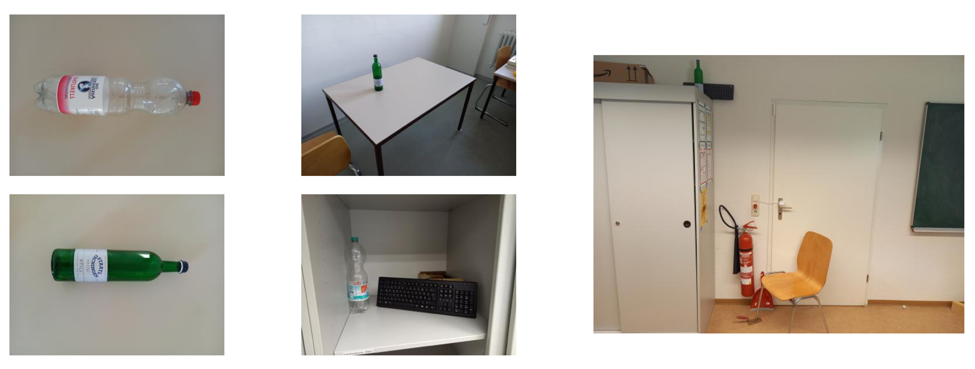
An example of the images for each complexity level, which includes, among other things, the object class bottle, can be found in Figure 3. From these 4 complexity levels, two further variants can be derived. The variant all includes the 1542 images from easy, medium, and hard, whereas all_aug contains the 4222 images from easy, medium, and hard_aug. The annotation of the images was done using bounding boxes and the software used was Roboflow [44]. The images and annotations are available at [45].

• Usage of GenAI

For this study, the following generative AI models were used for the following purposes:

• DeepL was used for the translation from German to English.
• ChatGPTo3 and ChatGPT5 were used to support code generation in Python 3.10.11.

4. Experiments & Results

4.1. Determination of the Optimal Ground-Truth T-Values for All Used Datasets

As already mentioned in Section 3.1, the seven datasets, LVIS minival [12], mydataset, Open Images V7 [22,23], COCO [25], Pascal VOC [24], EgoObjects [26], and Objects365v1 [14], including some variants of these, are used for the investigations in this study. Since T can take the values $T\in \{0.4+0.05·u\mid u\in \mathbb{Z},0\le u\le 32\}$, 66 ECE values ($ECE@[IoU=0.5]$ and $ECE@[IoU=0.75]$, respectively) must be calculated for each dataset, which corresponds to 33 evaluation runs per dataset (one run per T-value). Furthermore, the resulting optimal T-values must also be distinct from each other, which is why as many different datasets as possible should be used. Therefore, the generation of data is difficult and time-consuming.

Table 2. Overview of the used datasets and the corresponding optimal T-values.

Dataset	# Images	# Classes	Shuffle, Seed	Train, Val, Test	Opt. T@IoU = 0.5	Opt. T@IoU = 0.75
LVIS minival	4809/5000	1203	-	val	0.60	0.55
mydataset_easy_half	400	10	yes, 17	test	1.55	1.55
mydataset_easy	800	10	-	test	1.55	1.55
mydataset_medium	670	10	-	test	1.20	1.20
mydataset_hard	72	10	-	test	1.60	1.50
mydataset_hard_aug	2752	10	-	test	1.25	1.20
mydataset_all	1542	10	-	test	1.35	1.35
mydataset_all_aug	4222	10	-	test	1.25	1.25
Open Images val_1	7196/8000	601	no	val	0.65	0.60
Open Images val_2	7196/8000	530	no	val	0.70	0.60
Open Images val_3	17,921/20,000	558	yes, 60	val	0.70	0.60
Open Images train_1	10,000	514	no	train	0.70	0.60
Open Images train_2	9000	501	yes, 51	train	0.70	0.60
Open Images train_3	5000	442	yes, 22	train	0.75	0.65
COCO train_1	20,000	80	no	train	0.90	0.90
COCO train_2	12,000	80	yes, 76	train	0.90	0.90
COCO train_3	6000	80	yes, 75	train	0.90	0.90
COCO val	5000	80	-	val	0.90	0.90
Pascal VOC val	5823	20	-	val	0.80	1.20
Pascal VOC train	5717	20	-	train	0.80	1.25
Pascal VOC tainval	11,540	20	-	trainval	0.80	1.25
EgoObjects val	5000	637	yes, 33	val	0.55	0.55
EgoObjects train	6000	637	yes, 58	train	0.55	0.55
Objects365 tiny val	622	65	-	val	1.20	1.15
Objects365 tiny train	8688	65	-	train	1.20	1.15

provides an overview of the different datasets, including their variants. The variations relate to the number of images (# images), the number of classes (# classes), whether the training, validation, or test dataset was used (train, val, test), and whether the images were selected at random (shuffle, seed). If the images were selected at random, the corresponding seed is also specified. For the Open Images variations, only a subset of the training and validation dataset is used; the same applies to EgoObjects and the COCO training dataset. Since not all images are fully annotated in LVIS minival and Open Images, the column “# images” always shows the actual number of annotated images (e.g., 4809 for LVIS minival) and the total number of images (e.g., 5000 for LVIS minival). In the case of Open Images and COCO, the images and annotations were extracted using the fiftyone library [46], while for EgoObjects, the Python module random was used to draw images at random. The dataset mydataset_easy_half was generated by randomly selecting exactly half of the images from mydataset_easy, where each object class continues to be represented equally often. A total of 25 different datasets are used.

Also shown in Table 2 are the optimal T-values for the two IoU thresholds $IoU=0.5$ and $IoU=0.75$, which result in the minimum ECE values $ECE@[IoU=0.5]$ and $ECE@[IoU=0.75]$ of the 33 evaluation runs per dataset. As can be seen, the optimal T-values differ between the different datasets. Each dataset also has the corresponding logit distribution, which was determined at $T=1$ (see Section 3.1). Therefore, each of the 25 datasets can be assigned a data pair consisting of the two optimal T-values and the logit distribution.

4.2. Relationship Between the Logit Distribution and the Optimal T-Values

The first step in investigating the relationship between logit distributions and optimal T-values is to visually compare the distributions of the selected datasets. The Table 2 shows that the datasets mydataset_easy and mydataset_easy_half have exactly the same optimal T-values, $opt.T@[\mathrm{IoU}=0.5]=1.55$ and $opt.T@[\mathrm{IoU}=0.75]=1.55$. Since the optimal T-values of these two datasets are the same, the underlying logit distributions should also be similar. This is verified by the representation of the 4 plots, box plot, Q-Q plot, histogram and ECDF plot, in Figure 4.

The two box plots of the logit distributions of mydataset_easy and mydataset_easy_half look similar because the median, IQR, and whiskers are in a comparable position. The line histograms also have a similar shape. The quantiles plotted on the Q-Q plot are almost all on the 45° line, and the ECDFs of the two distributions are also almost identical. From this visual analysis, it can be concluded that the two logit distributions are similar.

Looking at two datasets with different optimal T-values, first mydataset_easy with $opt.T@[\mathrm{IoU}=0.5]=1.55$ and $opt.T@[\mathrm{IoU}=0.75]=1.55$ and second Open Images train_3 with $opt.T@[\mathrm{IoU}=0.5]=0.75$ and $opt.T@[\mathrm{IoU}=0.75]=0.65$, it is clear that the box plots, line histograms, and ECDF plots differ significantly from one another (see Figure 5). It should be noted that 500,000 samples were randomly selected (without replacement) from the logit distribution of Open Images train_3 to display the line histogram, as otherwise the line histogram of mydataset_easy would be much noisier. Also in the Q-Q plot, there is a clear deviation from the 45° line. This means that the two logit distributions of the datasets mydataset_easy and Open Images train_3 do not show any similarities. This simple analysis already provides an initial indication that similar logit distributions result in identical optimal T-values and that different distributions also have different T-values.

Using the Cramer-von-Mises two-sample test, further datasets are tested against each other with regard to equal logit distributions. As already mentioned in Section 3.1, there are no statistically significant differences in the distributions if $p>0.05$. For this test, the logit distributions of some datasets, such as Open Images or LVIS minival, are not considered, as these consist of several million logits. The problem here is that according to [47,48], even the smallest deviations become statistically significant in large samples, and thus the p value approaches 0, even if there are no practically significant differences. However, the Cramer-von-Mises two-sample test is sufficient for an initial assessment.

In Figure 6, all logit distributions of some selected datasets were tested against each other. In doing so, only the distributions of mydataset_easy and mydataset_easy_half and of Pascal VOC train and Pascal VOC trainval have the same optimal T-values (see Table 2). The results show that the Cramer-von-Mises test between the logit distributions of datasets with the same optimal T-values yields a p-value that is greater than 0.05 (these values are highlighted in bold). In all other cases, p is clearly below 0.05. The results of this comparison are a further proof that there is a correlation between the logit distributions and the optimal T-values.

Further evidence that similar logit distributions can be assigned the same optimal T-values is provided by EMD and Cliff’s Delta in Figure 7. For all datasets that result in the same optimal T-values, the underlying logit distributions have very small EMD values. For example, the datasets Open Images train_2 and Open Images val_2 both have optimal T-values of $opt.T@[\mathrm{IoU}=0.5]=0.70$ and $opt.T@[\mathrm{IoU}=0.75]=0.60$, and the resulting EMD has a value of 0.0195. This is very low compared to EMD values for logit distributions with unequal optimal T-values. In general, the EMD of distributions with equal optimal T-values are less than 0.025 and are thus highlighted in bold in Figure 7. The remaining EMD values are above 0.1.

Since calculating Cliff’s delta is very computationally intensive, it was determined using m-out-of-n bootstrap [49,50]. To do this, 20,000 samples were drawn with replacement from each of the two distributions to be compared; afterwards, Cliff’s delta was calculated, and this procedure was repeated for 2000 bootstrap runs. Figure 7 shows the median and the 95% confidence intervals. This clearly shows that the median and confidence intervals for logit distributions with the same optimal T-values take the lowest values. The Cliff’s delta confidence interval for these distributions has the smallest width and the Cliff’s delta median is also very low. From this, it can be deduced that modeling this correlation is the next reasonable step.

4.3. Prediction of the Optimal T-Values

As already explained in Section 4.1, generating data pairs is difficult and time-consuming. As a reminder, a data pair of a dataset consists of the optimal T-values and the logit distribution at $T=1$. For this reason, ML models that do not rely on huge amounts of training data are needed for modeling. Some models that meet this requirement are listed in [51]. These include Support Vector Machine (SVM) and Gaussian Process Regression (GPR), among others. In [52], it is shown that Kernel Ridge Regression (KRR) is also a powerful model and can outperform SVM. Therefore, the three models SVM, GPR, and KRR were selected for this investigation.

According to Figure 2, the respective ML model is given a logit distribution as input, from which the optimal T-values are predicted. Bootstrap is used to evaluate the stability of the model performance of the predictions. The number of bootstrap runs is set to $S=1000$. Exactly 25 data pairs are randomly drawn with replacement from the data pairs in Table 2, which are used as training data. The remaining data is used for testing. After all runs, the errors $MAE@[IoU=\delta ]$, $RMSE@[IoU=\delta ]$, and $R^2@[IoU=\delta ]$ can be derived, as described in Section 3.1.

The accuracy of the predictions depends not only on the selection of a suitable ML model, but also on its parameters. For KRR and SVM, the hyperparameter $\gamma$ was defined according to [53], i.e., $\gamma \in \{e^{-10},e^{-9},\dots ,e^0\}$. The hyperparameters $\alpha$ (KRR) and C (SVM) are defined as $\alpha ,C\in \{e^{-10},e^{-9},\dots ,e^{10}\}$. Furthermore, the parameter $\epsilon$ of the support vector machine can take the values $\{0.01,0.1\}$. The determination of the optimal hyperparameters of KRR and SVM is carried out by Grid Search, i.e., all possible combinations of the defined hyperparameters are tested, and Leave-One-Out cross-validation, where always exactly one data pair (from all data pairs in the training data) is used as a test sample and the remaining data pairs continue to be used as training samples. Each data pair appears exactly once as a test sample. The models are optimized during the training on the MAE, more precisely, a maximization of the negative MAE is aimed for. An RBF (radial basis function) kernel is used for all models (KRR, SVM, and GPR). Before the various ML models are trained, the x-values of the data pairs, i.e., the summary statistics of the logit distributions, are also scaled by the mean and the standard deviation. The other settings and parameters of KRR, SVM and GPR are based on the scikit-learn [54] standard implementation in Python. Further information on how the ML models KRR, SVM, and GPR work is listed in [55].

To map the logit distributions, in an initial investigation, based on [34], the summary statistics mean, standard deviation (std), coefficient of variation (CV), skewness, kurtosis, IQR, and median are defined. The results are listed in

Table 3. Error metrics RMSE, MAE, and R² after predicting the T-values for the IoU thresholds 0.5 and 0.75 using bootstrap ($S=1000$) and the summary statistics: mean, std, CV, skewness, kurtosis, IQR, and median. The best results are highlighted in bold.

Model	MAE@[IoU = 0.5]	RMSE@[IoU = 0.5]	R2@[IoU = 0.5]	MAE@[IoU = 0.75]	RMSE@[IoU = 0.75]	R2@[IoU = 0.75]
KRR	0.117 [0.050–0.410]	0.175 [0.066–0.600]	0.667 [−3.255–0.932]	0.094 [0.036–0.382]	0.148 [0.050–0.623]	0.787 [−2.790–0.971]
GPR	0.125 [0.036–0.457]	0.200 [0.053–0.687]	0.556 [−4.818–0.964]	0.105 [0.036–1.000]	0.167 [0.052–1.079]	0.722 [−10.474–0.973]
SVM	0.112[0.033–0.315]	0.184[0.046–0.471]	0.626[−2.108–0.963]	0.086[0.018–0.310]	0.155[0.033–0.459]	0.766[−1.244–0.987]

, where the best results are highlighted in bold. Based on the results, it is clear that SVM is the most powerful model, as both the median is very low and the confidence intervals (CI) are the narrowest. In general, SVM predictions have the highest stability compared to the other models. KRR also performs well, even though the median is slightly better in some cases, the confidence intervals are usually larger. GPR performs the worst.

However, the error metrics can be further reduced by using the summary statistics kurtosis, skewness, Q0.125, Q0.25, Q0.375, Q0.5, Q0.625, Q0.75, Q0.875, as suggested in [34], to map the logit distribution.

Table 4. Error metrics RMSE, MAE, and R² after predicting the T-values for the IoU thresholds 0.5 and 0.75 using bootstrap ($S=1000$) and the summary statistics: kurtosis, skewness, Q0.125, Q0.25, Q0.375, Q0.5, Q0.625, Q0.75, and Q0.875. The best results are highlighted in bold.

Model	MAE@[IoU = 0.5]	RMSE@[IoU = 0.5]	R2@[IoU = 0.5]	MAE@[IoU = 0.75]	RMSE@[IoU = 0.75]	R2@[IoU = 0.75]
KRR	0.085 [0.027–0.396]	0.139 [0.042–0.645]	0.784 [−3.156–0.981]	0.075 [0.025–0.423]	0.123 [0.038–0.673]	0.852 [−2.828–0.985]
GPR	0.112 [0.028–0.492]	0.181 [0.042–0.737]	0.647 [−4.574–0.976]	0.089 [0.020–0.955]	0.147 [0.033–1.034]	0.783 [−8.430–0.989]
SVM	0.090 [0.025–0.406]	0.152 [0.039–0.640]	0.752 [−3.399–0.979]	0.073 [0.017–0.367]	0.131 [0.029–0.575]	0.840 [−2.024–0.991]

shows the results, with KRR and SVM performing best. For an IoU threshold of 0.5, KRR is slightly better than SVM. In terms of MAE, KRR has an median error of 0.085, which is relatively low, with a CI of [0.027–0.396]. The CI is narrower compared to SVM and GPR, which means that KRR provides the most stable and reliable predictions. The same applies to the RMSE, even though the two confidence intervals of KRR and SVM are almost identical here. The median RMSE is also relatively low (0.139). However, the widths of the confidence intervals are generally relatively large, with a value of 0.369 for the MAE and 0.603 for the RMSE, considering that the step size of the T-values is 0.05 and T can take a minimum value of 0.4 and a maximum value of 2.0. The KRR model performance therefore varies between the different bootstrap datasets. The R² score yields similar results. Here, the median of KRR is the best with a value of 0.784 compared to the other models, as this should be as close to 1 as possible. Looking at the width of the confidence interval (4.137), relatively large fluctuations in the predictions are to be expected here as well. How well the model can explain the variance of the dependent variable based on the summary statistics compared to a simple application of the mean therefore varies. Similar results are obtained for an IoU threshold of 0.75, with the difference that SVM is the most powerful. The median values are relatively low, while the width of the confidence intervals is relatively high.

In general, it can therefore be concluded that the median values of the error metrics indicate minor deviations between the predicted T-values and the true optimal T-values. However, the deviations vary depending on the bootstrap dataset.

Nevertheless, the results of this study show that there is a correlation between the logit distributions and the optimal T-values. Even though the results may vary depending on the data, a modeling of this correlation is possible using ML models, with SVM and KRR proving to be the best models.

• Which summary statistics (features) are most relevant?

The following analysis will examine which summary statistics (features) are most relevant for predicting T-values, whether and to what extent the features can be reduced, and which features worsen the prediction.

Table 4 shows that the nine summary statistics kurtosis, skewness, Q0.125, Q0.25, Q0.375, Q0.5, Q0.625, Q0.75, and Q0.875 provide the best results, i.e., the best medians and the best confidence intervals, after 1000 bootstrap runs. KRR and SVM perform similarly well, so only KRR is used for the following investigations, and due to the high computational effort, the number of bootstrap runs is reduced to $S=50$. In a first step, all nine features are considered individually and their influence on the stability and accuracy of the prediction errors is examined. In addition, all error metrics of all features are calculated again together for 50 bootstrap runs as a reference. The first finding can already be derived from the results in

Table 5. Error metrics RMSE, MAE, and R₂ after predicting the T-values for the IoU thresholds 0.5 and 0.75 using bootstrap ($S=50$). The type and number of features (summary statistics) vary, with all features being considered individually, except for all (all nine features are taken into account). All error metrics were calculated only for the predictions of KRR.

Features	MAE@[IoU = 0.5]	RMSE@[IoU = 0.5]	R2@[IoU = 0.5]	MAE@[IoU = 0.75]	RMSE@[IoU = 0.75]	R2@[IoU = 0.75]
all	0.081 [0.025–0.445]	0.137 [0.043–0.675]	0.786 [−3.648–0.982]	0.077 [0.019–0.515]	0.128 [0.033–0.735]	0.846 [−4.291–0.988]
kurtosis	0.307 [0.160–2.416]	0.407 [0.206–3.885]	−0.547 [−173.545–0.301]	0.306 [0.157–1.591]	0.438 [0.198–2.376]	−0.435 [−51.757–0.433]
skewness	0.268 [0.157–3.161]	0.378 [0.181–7.713]	−0.559 [−650.026–0.512]	0.346 [0.142–3.096]	0.439 [0.225–7.295]	−0.609 [−642.533–0.449]
Q0.125	0.136 [0.077–1.812]	0.195 [0.095–3.554]	0.528 [−94.543–0.883]	0.131 [0.072–1.915]	0.179 [0.099–3.807]	0.580 [−112.626–0.898]
Q0.25	0.138 [0.092, 1.426]	0.193 [0.117, 2.921]	0.556 [−53.856, 0.847]	0.138 [0.083, 1.672]	0.192 [0.117, 3.367]	0.623 [−86.552, 0.844]
Q0.375	0.138 [0.079, 0.904]	0.182 [0.089, 1.844]	0.623 [−27.252, 0.889]	0.130 [0.083, 1.254]	0.182 [0.109, 2.516]	0.634 [−43.454, 0.865]
Q0.5	0.123 [0.061, 0.468]	0.156 [0.079, 0.810]	0.729 [−3.862, 0.926]	0.125 [0.070, 0.824]	0.169 [0.083, 1.663]	0.648 [−17.853, 0.927]
Q0.625	0.110 [0.058, 0.297]	0.161 [0.073, 0.454]	0.735 [−1.127, 0.921]	0.085 [0.032, 0.354]	0.131 [0.041, 0.678]	0.831 [−2.600, 0.975]
Q0.75	0.178 [0.062, 0.405]	0.255 [0.081, 0.518]	0.238 [−2.969, 0.886]	0.102 [0.040, 0.233]	0.143 [0.051, 0.312]	0.819 [−0.198, 0.973]
Q0.875	0.162 [0.101, 1.021]	0.234 [0.123, 1.626]	0.355 [−47.577, 0.829]	0.131 [0.053, 0.910]	0.199 [0.096, 1.463]	0.621 [−26.897, 0.890]

. When viewed individually, all quantile-features have relatively good median values and confidence intervals, which are significantly better than those of kurtosis and skewness. Particularly noteworthy are the features Q0.625 for the IoU threshold value 0.5 and Q0.75 for the IoU threshold value 0.75, whose confidence intervals already exceed those of the reference (all features).

In the next step, the sequential forward selection (SFS) [56,57] method is applied to select the best feature pairs. SFS is applied without floating. Overall, this method determines the best 2, 3, …, 6 feature combinations for the respective IoU thresholds while minimizing the median MAE.

Table 6. Error metrics RMSE, MAE, and R² after predicting the T-values for the IoU thresholds 0.5 and 0.75 using bootstrap ($S=50$). SFS was used to determine the best 2, 3, …, 6 feature combinations in terms of minimizing the median MAE. The smallest errors and thus the best feature combinations for the respective IoU thresholds are highlighted in bold. All error metrics were calculated only for the predictions of KRR.

Best Features IoU = 0.5	MAE@[IoU = 0.5]	RMSE@[IoU = 0.5]	R2@[IoU = 0.5]	Best Features IoU = 0.75	MAE@[IoU = 0.75]	RMSE@[IoU = 0.75]	R2@[IoU = 0.75]
Q0.125, Q0.625	0.067 [0.017, 0.300]	0.095 [0.029, 0.566]	0.889 [−1.439, 0.991]	Q0.25, Q0.75	0.048 [0.017, 0.377]	0.074 [0.029, 0.745]	0.949 [−3.253, 0.991]
Q0.125, Q0.625, Q0.75	0.063 [0.018, 0.255]	0.095 [0.034, 0.430]	0.858 [−0.768, 0.986]	Q0.125, Q0.25, Q0.75	0.055 [0.013, 0.296]	0.080 [0.025, 0.518]	0.943 [−1.143, 0.995]
Q0.125, Q0.375, Q0.625, Q0.75	0.074 [0.025, 0.249]	0.114 [0.038, 0.444]	0.805 [−0.854, 0.980]	Q0.125, Q0.25, Q0.5, Q0.75	0.059 [0.015, 0.314]	0.098 [0.028, 0.573]	0.878 [−1.572, 0.991]
Q0.125, Q0.375, Q0.625, Q0.75, Q0.875	0.079 [0.020, 0.311]	0.122 [0.040, 0.552]	0.839 [−1.317, 0.981]	Q0.125, Q0.25, Q0.375, Q0.5, Q0.75	0.055 [0.017, 0.361]	0.087 [0.030, 0.659]	0.926 [−2.342, 0.989]
Q0.125, Q0.25, Q0.375, Q0.625, Q0.75, Q0.875	0.079 [0.020, 0.293]	0.119 [0.033, 0.537]	0.835 [−1.146, 0.985]	Q0.125, Q0.25, Q0.375, Q0.5, Q0.625, Q0.75	0.056 [0.015, 0.361]	0.079 [0.035, 0.633]	0.934 [−1.711, 0.990]

shows the best feature combinations for each IoU threshold. The best results in terms of the median and confidence interval are highlighted in bold and include three features for the IoU values 0.5 (Q0.125, Q0.625, Q0.75) and 0.75 (Q0.125, Q0.25, Q0.75). It can be seen that the feature combination Q0.125 and Q0.75 works particularly well. Compared to the reference (all nine features), the median of MAE, RMSE, and R² has improved, as have the corresponding confidence intervals for both IoU thresholds.

The two best feature combinations of the respective IoU threshold are finally examined for 1000 bootstrap runs in order to have a fair comparison with Table 4. The results in

Table 7. Error metrics RMSE, MAE, and R² after predicting the T-values for the IoU thresholds 0.5 and 0.75 using bootstrap ($S=1000$). The error metrics of the two best feature combinations, which were determined using SFS, are calculated. All error metrics were calculated only for the predictions of KRR.

Best Features	MAE@[IoU = 0.5]	RMSE@[IoU = 0.5]	R2@[IoU = 0.5]	MAE@[IoU = 0.75]	RMSE@[IoU = 0.75]	R2@[IoU = 0.75]
Q0.125, Q0.625, Q0.75	0.057 [0.015–0.375]	0.088 [0.029–0.651]	0.904 [−2.541–0.989]	0.045 [0.010–0.344]	0.071 [0.022–0.561]	0.952 [−1.867–0.995]
Q0.125, Q0.25, Q0.75	0.056 [0.015–0.417]	0.087 [0.027–0.708]	0.904 [−3.190–0.990]	0.050 [0.013–0.414]	0.078 [0.025–0.710]	0.941 [−3.142–0.993]

show that these three features are sufficient to achieve similarly good or even better results compared to the error metrics of the KRR model in Table 4. From this, it can be concluded that the features can be significantly reduced without any deterioration in the predictions. In addition, Table 6 shows that the features kurtosis and skewness are not included in the best feature combinations, only the quantile features. Kurtosis and skewness are therefore of rather low relevance for mapping the logit distributions.

4.4. Investigation of the mAP and the ECE

In order to finally determine the influence of temperature scaling,

Table 8. ECE [%] and mAP [%] of the different datasets—the ECE and mAP are calculated once for $T=1.0$, i.e., no temperature scaling was applied, and contrasted with the ECE and mAP of the respective optimal T-values of the IoU thresholds 0.5 and 0.75. A green highlighting of the mAP indicates an improvement in the mAP, a red highlighting indicates a deterioration, and blue indicates no change.

Dataset	T = 1.0			opt. T-Wert@[IoU = 0.5]			opt. T-Wert@[IoU = 0.75]
	mAP	ECE@0.5	ECE@0.75	mAP	ECE@0.5	ECE@0.75	mAP	ECE@0.5	ECE@0.75
LVIS minival	35.5	5.43	5.75	35.4	1.95	2.34	35.2	1.99	2.21
mydataset_easy_half	47.4	3.33	3.33	49.7	0.27	0.26	49.7	0.27	0.26
mydataset_easy	45.7	3.45	3.44	48.1	0.27	0.27	48.1	0.27	0.27
mydataset_medium	54.8	0.98	0.81	55.2	0.12	0.16	55.2	0.12	0.16
mydataset_hard	27.2	3.44	2.96	27.9	0.18	0.33	27.8	0.36	0.16
mydataset_hard_aug	47.0	1.07	0.90	47.4	0.09	0.16	47.3	0.16	0.08
mydataset_all	45.0	1.85	1.70	45.9	0.15	0.16	45.9	0.15	0.16
mydataset_all_aug	47.6	1.21	1.06	48.1	0.11	0.13	48.1	0.11	0.13
Open Images val_1	41.0	3.37	3.78	40.7	0.96	1.28	40.3	1.28	1.10
Open Images val_2	41.2	3.17	3.59	41.0	0.94	1.43	40.5	1.39	1.07
Open Images val_3	40.1	3.23	3.66	39.9	0.94	1.43	39.5	1.42	1.09
Open Images train_1	42.6	3.47	3.90	42.3	1.39	1.90	41.2	1.84	1.69
Open Images train_2	43.9	3.57	4.09	43.7	1.18	1.77	43.0	1.85	1.50
Open Images train_3	46.6	3.01	3.55	46.4	1.25	1.88	46.1	1.8	1.53
COCO train_1	45.6	0.87	1.47	45.6	0.61	1.43	45.6	0.61	1.43
COCO train_2	45.8	0.89	1.49	45.8	0.63	1.45	45.8	0.63	1.45
COCO train_3	46.0	0.88	1.47	45.9	0.62	1.43	45.9	0.62	1.43
COCO val	45.0	0.89	1.49	45.0	0.63	1.44	45.0	0.63	1.44
Pascal VOC val	63.1	0.93	1.37	63.0	0.77	1.96	63.1	0.99	1.13
Pascal VOC train	63.0	0.95	1.42	62.9	0.77	2.08	63.0	1.03	1.17
Pascal VOC tainval	62.9	0.94	1.39	62.8	0.75	2.02	63.0	1.02	1.15
EgoObjects val	38.3	5.40	5.56	37.8	1.67	1.87	37.8	1.67	1.87
EgoObjects train	35.8	5.31	5.47	35.2	1.62	1.84	35.2	1.62	1.84
Objects365 tiny val	33.8	0.63	0.53	35.2	0.10	0.24	34.9	0.12	0.15
Objects365 tiny train	34.4	0.80	0.58	36.0	0.04	0.17	35.8	0.14	0.06

shows the mAP and the ECE before and after the calibration with the optimal T-values. The influence of each optimal T-value on the mAP and ECE is considered individually, i.e., for each optimal T-value $opt.T@[IoU=0.5]$ and $opt.T@[IoU=0.75]$, the mAP and the $ECE@[IoU=0.5]$ and $ECE@[IoU=0.75]$ are calculated. For better clarity, only the short form of $ECE@[IoU=0.5]$ and $ECE@[IoU=0.75]$ is used, i.e., $ECE@0.5$ and $ECE@0.75$. The calculation of the mAP was performed using mmdet.LVISMetric, which is why all annotation files of the datasets were converted to the LVIS format. For the datasets COCO, Pascal VOC and mydataset, the list neg_category_ids contains all class IDs for which there are no annotations in the respective image. Since the labeling for Open Images and Objects365 is not exhaustive, there is no entry in the list neg_category_ids for these datasets. In Table 8, the mAP values for those where there was a decrease are shown in red and those where the mAP increased are shown in green, whereas no changes are highlighted in blue. The ECE and the mAP are both expressed as percentages. The optimal T-values for each dataset can be found in Table 2.

Based on Table 8, it can be seen that in all cases where the optimal T-value is less than 1 ($T<1$), the mAP is slightly reduced or remains unchanged. The largest reduction is 1.4% for the Open Images train_1 dataset (IoU = 0.75). In this case, the optimal T-value is $opt.T@[IoU=0.75]=0.60$ and the mAP before and after calibration is 42.6% and 41.2%, respectively. But in general, for the case $T<1$, the influence on the mAP is rather negligible. For optimal T-values that are greater than 1 ($T>1$), temperature scaling results in an increase in mAP, with the exception of the Pascal VOC val and Pascal VOC train datasets, where the mAP does not change. The strongest increase occurred in the mydataset_easy dataset, where the mAP improved by 2.4%. For most other datasets, the increase in mAP is rather small.

The ECE has been reduced by temperature scaling with the optimal T-values in all cases, i.e., a better calibration has been achieved. For the datasets LVIS minival, mydataset, Open Images, EgoObjects, and Objects365 the effect on the ECE is greatest, with a reduction of up to 3.54% (in the case of LVIS minival). The influence is slightly lower for Pascal VOC and COCO; however, it should be noted that the ECE is already relatively low at $T=1$. It is also interesting to note that despite a sigmoid activation of the logits (see Equation (2)), in which all logits are considered independently of each other, the ECE can be improved and the mAP remains largely unaffected.

When looking at the mAP in Table 8, it can be seen that it varies greatly depending on the dataset. One possible reason for this, among others, could be the different annotations and labels used in the various datasets. Therefore, the annotation of objects is not trivial. For example, one could annotate a light switch with the frame, as it is usually done, but also without the frame. A multiple power outlet could be annotated completely as one power outlet or even each outlet individually. This is particularly interesting if a different annotation strategy was used for the pre-training dataset of the model. This inconsistency then contributes to part of the uncertainty (data uncertainty) of the model predictions.

As mentioned in Section 3.1, other metrics to indirectly measure the calibration of the model are Brier Score (BS) and Sigmoid Cross-Entropy (SiCE), which will be briefly discussed below. The equations for calculating BS and SiCE are defined in the Appendix A in Equations (A1) and (A2), respectively, based on [40,41] (BS) and [42,43] (SiCE). The corresponding notation is defined in Section 2.3.

Table A1. BS [%] of the different datasets—BS is calculated once for $T=1.0$, i.e., no temperature scaling was applied, and contrasted with the BS of the respective optimal T-values of the IoU thresholds 0.5 and 0.75. The optimal T-values are the ECE optimized ones.

Dataset	T = 1.0		opt. T-Wert@[IoU = 0.5]		opt. T-Wert@[IoU = 0.75]
	BS@0.5	BS@0.75	BS@0.5	BS@0.75	BS@0.5	BS@0.75
LVIS minival	2.40	2.23	2.59	2.34	2.93	2.64
mydataset_easy_half	4.66	4.68	0.91	0.91	0.91	0.91
mydataset_easy	4.70	4.70	0.89	0.89	0.89	0.89
mydataset_medium	2.38	2.23	1.05	0.99	1.05	0.99
mydataset_hard	4.58	4.04	1.25	1.07	1.31	1.13
mydataset_hard_aug	2.48	2.32	0.95	0.88	1.14	1.06
mydataset_all	3.28	3.11	0.99	0.93	0.99	0.93
mydataset_all_aug	2.63	2.49	1.03	0.96	1.03	0.96
Open Images val_1	1.81	1.52	2.09	1.67	2.39	1.90
Open Images val_2	1.81	1.51	1.96	1.57	2.51	2.00
Open Images val_3	1.86	1.56	1.99	1.60	2.54	2.02
Open Images train_1	1.94	1.66	2.15	1.77	2.78	2.29
Open Images train_2	2.15	1.79	2.30	1.84	2.87	2.29
Open Images train_3	2.17	1.79	2.37	1.90	2.91	2.32
COCO train_1	1.90	1.84	2.42	2.34	2.42	2.34
COCO train_2	1.91	1.84	2.44	2.35	2.44	2.35
COCO train_3	1.92	1.85	2.44	2.35	2.44	2.35
COCO val	1.95	1.87	2.47	2.38	2.47	2.38
Pascal VOC val	1.37	1.49	2.97	3.27	0.70	0.76
Pascal VOC train	1.37	1.50	2.98	3.31	0.64	0.70
Pascal VOC tainval	1.37	1.50	2.97	3.29	0.63	0.68
EgoObjects val	1.97	1.89	2.14	2.02	2.14	2.02
EgoObjects train	1.92	1.83	2.09	1.94	2.09	1.94
Objects365 tiny val	1.73	1.55	0.86	0.76	1.01	0.90
Objects365 tiny train	2.05	1.83	0.95	0.85	1.14	1.02

and

Table A2. SiCE [%] of the different datasets – SiCE is calculated once for $T=1.0$, i.e., no temperature scaling was applied, and contrasted with the SiCE of the respective optimal T-values of the IoU thresholds 0.5 and 0.75. The optimal T-values are the ECE optimized ones.

Dataset	T = 1.0		opt. T-Wert@[IoU = 0.5]		opt. T-Wert@[IoU = 0.75]
	SiCE@0.5	SiCE@0.75	SiCE@0.5	SiCE@0.75	SiCE@0.5	SiCE@0.75
LVIS minival	10.82	10.31	10.38	9.35	11.69	10.47
mydataset_easy_half	20.31	20.45	4.14	4.16	4.14	4.16
mydataset_easy	20.74	20.81	4.06	4.07	4.06	4.07
mydataset_medium	9.61	8.95	4.46	4.23	4.46	4.23
mydataset_hard	20.84	18.28	5.70	4.95	5.99	5.20
mydataset_hard_aug	10.27	9.56	4.22	3.91	4.96	4.61
mydataset_all	14.01	13.27	4.47	4.24	4.47	4.24
mydataset_all_aug	10.97	10.32	4.56	4.28	4.56	4.28
Open Images val_1	8.55	7.61	9.01	7.26	10.24	8.16
Open Images val_2	8.43	7.47	8.44	6.86	10.72	8.52
Open Images val_3	8.63	7.65	8.54	6.95	10.82	8.61
Open Images train_1	8.71	7.79	8.91	7.40	11.41	9.31
Open Images train_2	9.52	8.42	9.47	7.70	11.87	9.42
Open Images train_3	9.31	8.07	9.66	7.83	11.87	9.41
COCO train_1	7.40	7.14	9.26	8.87	9.26	8.87
COCO train_2	7.46	7.16	9.31	8.90	9.31	8.90
COCO train_3	7.50	7.20	9.38	8.91	9.38	8.91
COCO val	7.60	7.26	9.47	9.01	9.47	9.01
Pascal VOC val	5.34	5.68	10.94	11.70	3.06	3.22
Pascal VOC train	5.32	5.70	10.86	11.79	2.86	3.02
Pascal VOC tainval	5.33	5.69	10.90	11.74	2.82	2.97
EgoObjects val	9.63	9.41	8.73	8.22	8.73	8.22
EgoObjects train	9.46	9.20	8.52	7.92	8.52	7.92
Objects365 tiny val	7.61	6.83	3.99	3.61	4.63	4.16
Objects365 tiny train	8.77	7.84	4.25	3.83	5.01	4.51

show the changes in these metrics depending on the T-value. As already seen for the ECE in Table 8, the metrics are calculated once for $T=1$ and once for the respective optimal T-values depending on the IoU thresholds. The optimal T-values are still those values that result in the lowest ECE. The calibration and reliability of the predictions are optimal if $BS=0$ and $SiCE=0$. The results show that BS and SiCE could always be reduced when the optimal T-value was greater than 1. In the case of T-values less than 1, the SiCE was improved in some cases and worsened in others. BS became worse in all cases. However, the T-values were also not optimized for these metrics.

5. Discussion and Conclusions

This paper examined how to determine the optimal T-value of the temperature scaling method for improving the model calibration of YOLO-World. To do this, the logit distributions of selected datasets were first compared with each other using visual representations (box plots, line histograms, Q-Q plots, and ECDF plots), a statistical test (Cramer-von-Mises two-sample test), the Earth mover’s distance (EMD) and the non-parametric effect size Cliff’s delta. The results showed that datasets with similar logit distributions also result in the same optimal T-values and datasets with different logit distributions result in different optimal T-values. The optimal T-value therefore depends on the underlying logit distribution, which was generated by YOLO-World. Based on this finding, the ML methods KRR, SVM, and GPR were utilized to model the relationship. Using the summary statistics kurtosis, skewness, Q0.125, Q0.25, Q0.375, Q0.5, Q0.625, Q0.75 and Q0.875, the logit distributions could initially be best described. The KRR and SVM models provide the best results with small median MAE and RMSE values and an R² median close to 1 for both IoU thresholds. However, the confidence intervals are relatively wide, which means that the performance of the models varies in terms of predicting the optimal T-values. For some bootstrap variations, the predictions are very accurate, while in other cases they are rather inaccurate. In further investigations using the KRR model, the nine summary statistics could be reduced to three, achieving the same and in some cases even better results.

The temperature scaling with the optimal T-value was able to improve the calibration error ECE in all cases and this without significantly reducing the mAP. A slight negative influence on the mAP is present in most datasets in which the optimal T-value is less than 1. However, for T-values greater than 1, the mAP is increased in most cases. The extent to which the ECE can be reduced depends on the dataset (see Section 4.4), i.e., in some cases the impact is greater, while in others only a slight improvement could be achieved. Temperature scaling thus proves to be a simple and, in some cases, effective method for improving the calibration of YOLO-World.

This study also showed that this approach has some disadvantages. Various datasets with different optimal T-values are required for training the ML models, as there is no optimal T-value that is the same for all datasets. Furthermore, an evaluation run must be carried out for each dataset and for each T-value in order to determine the optimal T-value, which is time-consuming. This approach is therefore less practical for models such as mm-Grounding DINO, as these models have a significantly higher inference time.

In conclusion, this study shows that there is a correlation between the optimal T-values and the logit distributions generated by YOLO World, which can be modeled using ML models. Through temperature scaling with the optimal T-values, the ECE could be reduced in all cases, with the extent depending on the dataset. The influence on the mAP is generally rather negligible, however a T-value less than 1 can lead to a decrease and a T-value greater than 1 can lead to an increase in the mAP.

In future work, further methods and approaches for improving the determination of confidence values for OVD models from the fields of calibration and uncertainty estimation should be tested and evaluated.