Improved DBSCAN-Based Electricity Theft Detection Using Spatiotemporal Fusion Features

Abstract

Electricity theft is a major source of non-technical losses in distribution networks, threatening both economic revenues and power supply reliability. This study addresses the identification of nodes exhibiting anomalous load behavior (anomalous nodes) in 10 kV distribution feeders. Based on the IEEE-33 bus benchmark system, the disturbance patterns induced by abnormal consumption are analyzed. The results show that voltage and current fluctuations intensify with increasing electrical distance from the power source, while branch loss peaks localize at the affected terminals and propagate unidirectionally along the power flow path. Building on these findings, an improved density-based spatial clustering of applications with noise (DBSCAN) method is proposed, integrating five spatial network features and sixteen temporal electrical features extracted from voltage, current, and power series. Prior to clustering, the features are standardized and reduced via principal component analysis (PCA), retaining over 90% of the cumulative variance. Validation on a hybrid dataset demonstrates that the proposed method achieves 90.7% accuracy, 87.5% recall, and an F1-score of 0.895, outperforming traditional K-means and approaching supervised CNN models without requiring labeled data. These results confirm the method’s robustness and suitability for practical deployment in distribution networks.

1. Introduction

Energy losses are inevitable throughout the process of electricity generation, transmission, and consumption. These losses can be categorized into technical losses (TL) and non-technical losses (NTL) [1,2]. TL primarily arise from inherent dissipation in transmission lines, substations, distribution systems, and metering processes required to maintain normal grid operation. Conversely, NTL primarily stems from abnormal electricity consumption behaviors, notably electricity theft at the distribution level, constituting controllable losses [3,4]. Global economic losses due to electricity theft are estimated to exceed USD 96 billion annually [5]. In China, NTL accounts for approximately 16% of total electricity generation, while in India, it exceeds 25% [6]. Even in developed countries, the corresponding losses are considerable, reaching about USD 10 billion in Canada and USD 6 billion in the United States [7]. Common theft techniques include line hooking, meter bypassing, and meter tampering [8]. Therefore, effective and accurate theft detection is essential for safeguarding utility revenues and ensuring distribution system reliability.

Traditional electricity theft detection relies on manual inspection and heuristic judgment, which are inefficient and lack precise localization. With the deployment of Advanced Metering Infrastructure (AMI) and the widespread installation of smart meters, utilities now have access to massive amounts of consumption data, providing the foundation for data-driven theft detection [9]. Existing methods can generally be divided into two categories: network-oriented and data-oriented approaches [10]. The former leverage the physical and topological characteristics of the distribution network, while the latter analyzes statistical and temporal patterns of customer load data.

Network-oriented methods typically utilize voltage, current, and other electrical measurements from distribution sensors, in combination with network topology, to identify abnormal nodes. Luan et al. proposed a “weight-dropped polling” state estimation method for theft detection [11]. Silva et al. developed a P-median model to optimize the placement of power-quality monitors [12]. Manito et al. introduced an Equivalent Operational Impedance (EOI) approach to distinguish TL and NTL using load-flow analysis [13]. Ferreira et al. employed node voltage and active/reactive power data to locate illegal connections [14]. Veeramani et al. utilized an IoT-based current comparison between distribution transformers and aggregated customer currents [15]. These approaches accurately represent the physical laws of distribution networks, directly reflect real operating conditions, and exhibit low dependence on customer-side data, making them interpretable and practically implementable in engineering applications.

Data-oriented methods focus on mining temporal consumption patterns such as daily energy usage and load fluctuations to identify abnormal behaviors. They can be further divided into supervised and unsupervised techniques [10]. Supervised approaches rely on labeled datasets to train models that distinguish between normal and theft behaviors. Ul Haq et al. developed a Deep Convolutional Neural Network (Deep-CNN) for theft detection [16]. Bai et al. proposed a dual-scale dual-branch CNN combined with a Gaussian-weighted Transformer [17]. Fernandes introduced a probabilistic Optimum-Path Forest (OPF) classifier [18]. Rajesh proposed a hybrid method combining Dynamic Time Warping (DTW) and k-Nearest Neighbor (k-NN) [19]. Punmiya et al. improved eXtreme Gradient Boosting (XGBoost) for theft detection under Time-of-Use (ToU) pricing [20]. Xia et al. adopted a Convolutional Long Short-Term Memory (ConvLSTM) model to capture both global and local temporal dependencies [21]. Supervised learning methods generally achieve higher accuracy and exhibit strong pattern recognition capabilities when sufficient labeled data are available.

Unsupervised approaches, on the other hand, detect anomalies by exploring intrinsic data structures without requiring labeled samples. Wu applied K-means clustering to analyze consumption patterns [22]. Peng et al. combined K-means and Local Outlier Factor (LOF) for anomaly detection [23]. Bondok et al. integrated K-means, autoencoders, and one-class SVM [24]. Tian et al. employed DBSCAN to detect anomalous energy use [25]; and Zheng et al. used density-Clust with local density and distance metrics to characterize abnormal patterns [26]. These unsupervised methods effectively eliminate the dependence on labeled datasets, discover hidden patterns autonomously, and offer strong generalization and scalability in real-world applications.

Although supervised methods generally achieve higher detection accuracy, electricity theft data are highly confidential within utilities, and large-scale labeling is both difficult and privacy-sensitive. Even when suspicious users are detected, on-site verification is still required. Therefore, unsupervised approaches that can detect anomalies from unlabeled data offer greater practical value. Additionally, most existing studies rely solely on consumption data without considering spatial information, such as the user’s position in the distribution feeder. This limitation weakens the model’s ability to represent electrical correlations across the network. Incorporating network topology into analysis can improve detection accuracy under the same amount of electrical measurement data.

To address these challenges, this study investigates electricity theft detection in 10 kV distribution feeders. The disturbance patterns of node voltage, branch current, and power loss under theft scenarios are analyzed, and an improved DBSCAN-based electricity theft detection method with spatiotemporal feature fusion is proposed. Spatially, five topological features are constructed based on the node adjacency matrix; temporally, sixteen load time-series features are extracted. The fused spatiotemporal features are then reduced via Principal Component Analysis (PCA), and DBSCAN clustering is applied to achieve unsupervised identification of nodes exhibiting anomalous load behavior (anomalous nodes).

The main contributions of this paper are as follows:

• Analyzes the impact of anomalous load behaviors on node voltage, branch current, and power loss in distribution feeders, providing physical insights and engineering guidance for theft detection in practical systems.
• Enables low-cost implementation relying solely on data collected from existing smart meters, without the need for additional monitoring devices.
• Proposes a spatiotemporal feature fusion approach that jointly captures electrical correlations in feeder topology and temporal load dynamics, enhancing the representational capacity of input features.
• Develops an unsupervised detection framework integrating PCA-based dimensionality reduction and DBSCAN clustering, effectively removing dependence on labeled or historical data.

The remainder of this paper is organized as follows. Section 2 introduces the benchmark distribution system and analyzes the impact of theft behaviors on electrical parameters. Section 3 describes the proposed improved DBSCAN-based detection method incorporating spatiotemporal fusion features. Section 4 provides case studies and performance evaluations. Section 5 discusses the practical application, significance, limitations, and potential future improvements of the proposed method. Finally, Section 6 concludes the paper.

2. Electrical Parameter Analysis of Single-Node and Multi-Node Anomalies in Distribution Networks

2.1. Benchmark Model Construction

The IEEE 33-bus distribution network is adopted as the benchmark model in this study due to its representative 10 kV radial structure and moderate network scale, which effectively balances modeling realism and computational efficiency for simulation-based theft analysis [27]. As shown in Figure 1, the system consists of 33 nodes and 32 feeder branches in a typical radial configuration.

Bus 1 serves as the slack (source) node. A single main feeder (trunk line) extends from Bus 1 to Bus 18, from which three lateral branches supply downstream consumer areas (Buses 19–33). The network parameters, including line impedances and load power vectors, are derived from the IEEE PES Test Feeder standard [28]. The detailed configuration parameters are listed in

Table 1. Benchmark Parameter Configuration of IEEE 33-Bus Distribution System.

Node $\mathit{i}$	Node $\mathit{j}$	Line Impedance/p.u.	Node $\mathit{j}$ Load/kW + j kVar	Node $\mathit{i}$	Node $\mathit{j}$	Line Impedance/p.u.	Node $\mathit{j}$ Load/kW + j kVar
1	2	0.0922 + j0.047	100 + j60	17	18	0.3720 + j0.5740	90 + j40
2	3	0.4930 + j0.2511	90 + j40	2	19	0.1640 + j0.1565	90 + j40
3	4	0.3660 + j0.1864	120 + j80	19	20	1.5042 + j1.3554	90 + j40
4	5	0.3811 + j0.1941	60 + j30	20	21	0.4095 + j0.4784	90 + j40
5	6	0.8190 + j0.7070	60 + j20	21	22	0.7089 + j0.9373	90 + j40
6	7	0.1872 + j0.6188	200 + j100	3	23	0.4512 + j0.3083	90 + j50
7	8	0.7114 + j0.2351	200 + j100	23	24	0.8980 + j0.7091	420 + j200
8	9	1.0300 + j0.7400	60 + j20	24	25	0.8960 + j0.7011	420 + j200
9	10	1.0440 + j0.7400	60 + j20	6	26	0.2030 + j0.1034	60 + j25
10	11	0.1966 + j0.0650	45 + j30	26	27	0.2842 + j0.1447	60 + j25
11	12	0.3744 + j0.1238	60 + j35	27	28	1.0590 + j0.9337	60 + j20
12	13	1.4680 + j1.1550	60 + j35	28	29	0.8042 + j0.7006	120 + j70
13	14	0.5416 + j0.7129	120 + j80	29	30	0.5075 + j0.2585	200 + j600
14	15	0.5910 + j0.5260	60 + j10	30	31	0.9744 + j0.9630	150 + j70
15	16	0.7463 + j0.5450	60 + j20	31	32	0.3105 + j0.3619	210 + j100
16	17	1.2890 + j1.7210	60 + j20	32	33	0.3410 + j0.5362	60 + j40

.

To address the scarcity of labeled datasets for electricity theft identification, this study constructs power flow analysis models for theft scenarios by proportionally reducing the injected power at selected nodes of the IEEE 33-bus system using open-source load data. Both single-node and multi-node theft cases are simulated under theft ratios of 0.2, 0.4, 0.6, and 0.8. The Newton–Raphson algorithm is used to solve the power flow equations.

Based on the simulation results, the impacts of electricity theft on network electrical parameters are analyzed. Typical patterns include voltage drop at anomalous nodes, current reduction in adjacent branches, and variations in power factor. These results provide essential support for the subsequent identification of anomalous nodes.

2.2. Parameters Under Normal Operating Conditions

Figure 2 depicts the voltage distribution characteristics of the IEEE-33 distribution network under normal operating conditions, solved via the Newton-Raphson power flow algorithm. As the electrical distance from the 11 kV source bus increases, the system exhibits a characteristic voltage gradient decay, with node voltage magnitudes decreasing in a stepwise manner along the feeder direction.

To facilitate comparative analysis of electrical parameter variations in the IEEE-33 distribution network model under theft conditions, the branches are systematically numbered (see

Table 2. Branch Numbering of the IEEE-33 Distribution Network.

Line ID	From Node	To Node	Line ID	From Node	To Node	Line ID	From Node	To Node	Line ID	From Node	To Node
Line1	1	2	Line9	9	10	Line17	17	18	Line25	6	26
Line2	2	3	Line10	10	11	Line18	2	19	Line26	26	27
Line3	3	4	Line11	11	12	Line19	19	20	Line27	27	28
Line4	4	5	Line12	12	13	Line20	20	21	Line28	28	29
Line5	5	6	Line13	13	14	Line21	21	22	Line29	29	30
Line6	6	7	Line14	14	15	Line22	3	23	Line30	30	31
Line7	7	8	Line15	15	16	Line23	23	24	Line31	31	32
Line8	8	9	Line16	16	17	Line24	24	25	Line32	32	33

for numbering conventions).

The key electrical parameters under normal conditions, including branch voltages, currents, and power losses, are presented in

Table 3. Electrical Parameters of Branches in the IEEE 33-Bus Distribution System.

Line ID	Voltage/V	Current/A	Power Loss /kW + j kVar	Line ID	Voltage/V	Current/A	Power Loss /kW + j kVar
Line1	36.72	210.34	7.07 + j3.12	Line17	5.83	4.92	0.02 + j0.03
Line2	179.30	187.11	29.90 + j15.23	Line18	7.10	18.09	0.10 + j0.09
Line3	95.76	134.61	11.49 + j5.85	Line19	47.62	13.58	0.48 + j0.43
Line4	94.72	127.87	10.79 + j5.50	Line20	9.88	9.06	0.06 + j0.07
Line5	233.79	124.75	22.08 + j19.06	Line21	9.22	4.53	0.03 + j0.03
Line6	65.37	58.38	1.105 + j3.65	Line22	45.88	48.48	1.84 + j1.25
Line7	62.01	47.61	2.80 + j0.92	Line23	86.59	43.69	2.97 + j2.34
Line8	80.79	36.78	2.41 + j1.73	Line24	43.12	21.88	0.74 + j0.58
Line9	74.73	33.71	2.06 + 1.46	Line25	25.78	65.34	1.50 + j0.76
Line10	10.99	30.64	0.32 + j0.11	Line26	34.51	62.48	1.92 + j9.79
Line11	19.13	28.00	0.51 + 0.17	Line27	145.83	59.63	6.52 + j5.75
Line12	79.59	24.60	1.54 + j1.21	Line28	105.25	56.97	4.52 + j3.94
Line13	32.85	21.18	0.42 + j0.55	Line29	49.89	50.58	2.25 + j1.15
Line14	19.44	14.19	0.21 + j0.18	Line30	55.40	23.35	0.92 + j0.91
Line15	17.94	11.21	0.16 + j0.12	Line31	12.49	15.13	0.12 + j0.14
Line16	30.04	8.06	0.15 + j0.19	Line32	3.95	3.59	0.008 + j0.012

, serving as a reference baseline for subsequent comparative studies of anomalous conditions.

2.3. Single-Node Anomaly Analysis

Based on the IEEE 33-bus distribution network model, a single-node anomaly scenario is constructed. The scenario selects the central feeder nodes (6 and 4) and secondary branch nodes (14 and 24) to investigate the variations in node voltages, branch currents, and branch power losses under theft conditions. The calculation formula for the rate of change is given in Equation (1), and the variations in complex power injections at the anomalous nodes are listed in

Table 4. Proportional Changes in Power Load of Anomalous Node.

No.	Node	Normal Power Load/kW + jkVar	Power at Theft Ratio r/kW + jkVar
			r1 = 0.2	r2 = 0.4	r3 = 0.6	r4 = 0.8
1	4	120 + j80	96 + j64	72 + j48	48 + j32	24 + j16
2	6	60 + j20	48 + j16	36 + j12	24 + j8	12 + j4
3	14	120 + j80	96 + j64	72 + j48	48 + j32	24 + j16
4	24	420 + j200	336 + j160	252 + j120	168 + j80	84 + j40

.

$$\Delta x_k(\%)=\left({\displaystyle \frac{x_k^{post}-x_x^{pre}}{x_k^{pre}}}\right)\times 100\%,$$

(1)

In Equation (1), $x_k^{pre}$ and $x_k^{post}$ denote the branch or node data before and after electricity theft, respectively.

(1)

Node Voltage Variation under Single-Node Anomalies

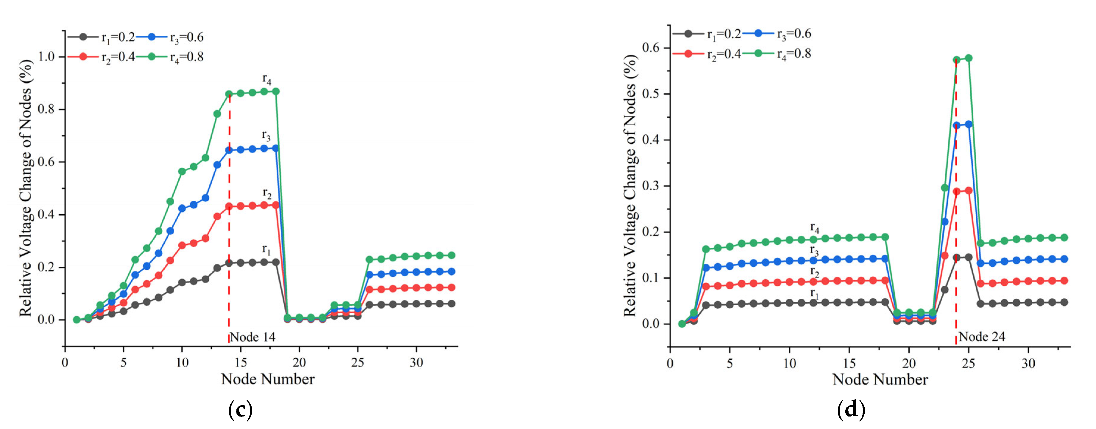
Figure 3a–d show the relative voltage changes in nodes in the IEEE-33 distribution network under a single-node anomaly. Upstream nodes (1–3) exhibit increasing voltage disturbances with electrical distance from the source, peaking at the anomalous node. In the middle and downstream sections of the main feeder (nodes 4–18), voltage fluctuations remain relatively stable, whereas branch lines (19–22, 23–25) follow disturbance patterns similar to their adjacent main feeder nodes. The radial network structure amplifies voltage variations at remote nodes due to higher impedance and sudden changes in theft current, causing significant Ohmic voltage drops.

Comparing Figure 3a–c with Table 4, the voltage change trends remain consistent as the theft ratio increases from 0.2 to 0.8. For instance, node 4 shows voltage change rates of 2.26%, 4.56%, 6.64%, and 9.11% corresponding to theft ratios of 0.2, 0.4, 0.6, and 0.8, respectively, demonstrating approximate linear proportionality. Node 17, located at the feeder terminus, also shows increasing changes of 2.47%, 4.94%, 7.39%, and 9.86%, indicating that theft has a network-wide impact. These results confirm that, under stable operation of other nodes, an increase in theft proportion leads to proportional voltage changes across the system.

(2)

Branch Current Variation under Single-Node Anomalies

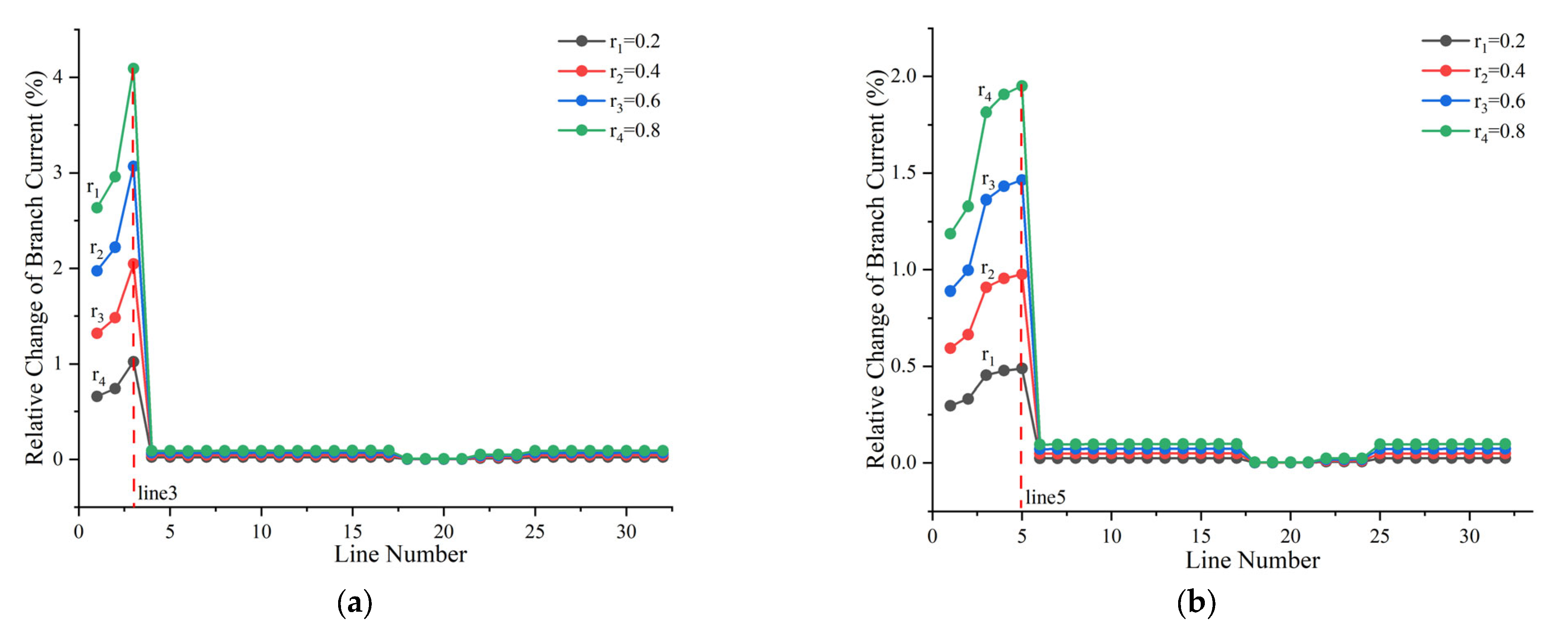
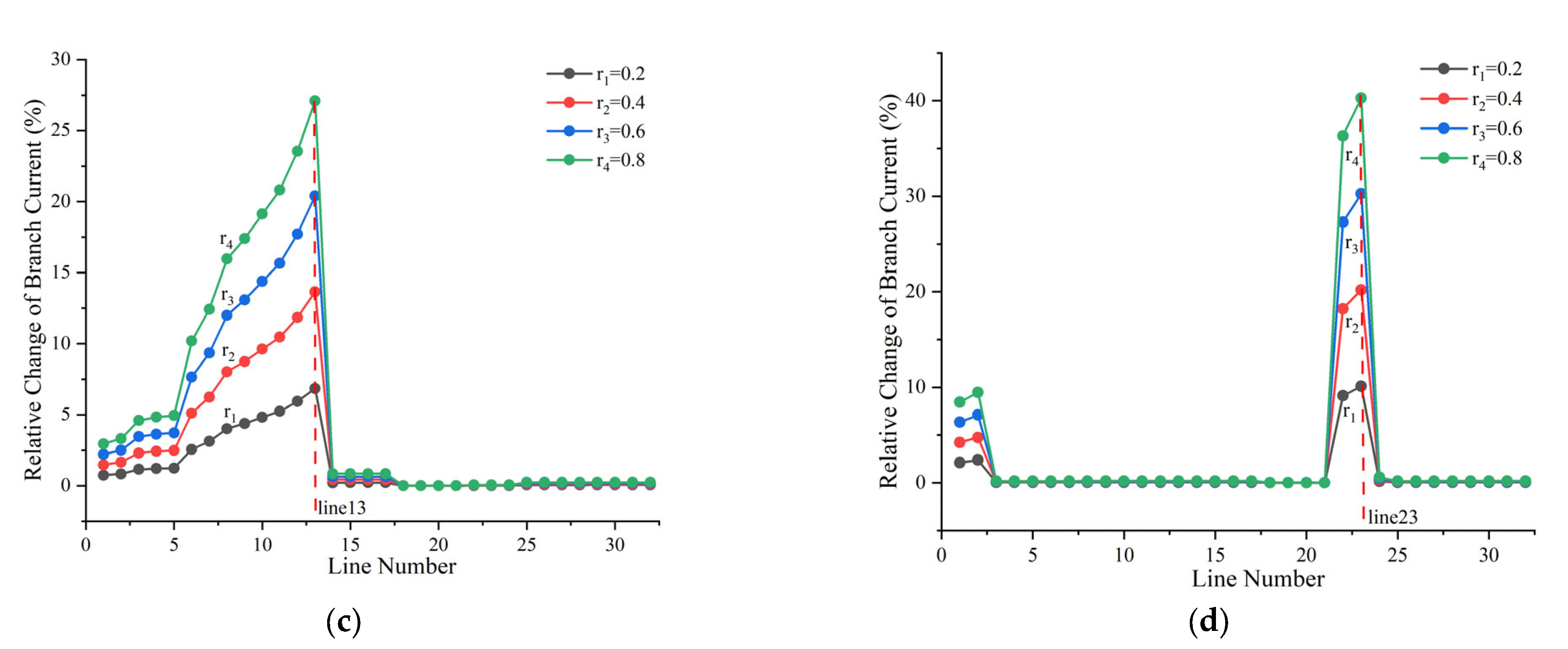
Figure 4a–d present relative changes in branch currents under single-node anomalies. In Figure 4a, upstream branches of the anomalous node exhibit increasing current changes along the feeder in the reverse direction, peaking at the terminal branch, while other branches show negligible fluctuations. A similar pattern is observed in Figure 4b. For remote-node theft (Figure 4c), the current variation gradient increases along the main feeder branches (Line 1–Line 13), while subsequent branches (Line 14–19, etc.) remain unchanged. In Figure 4d, proximal branch theft induces pronounced disturbances solely in upstream segments of the theft branches (Line 22–Line 24), with maximum change rates exceeding 40%.

(3)

Branch Power Loss Variation under Single-Node Anomalies

Based on the IEEE-33 distribution network benchmark model, the relative changes in branch power losses caused by a single-node anomaly at node 6 (near the source on the main feeder) and node 24 (end of the secondary branch) are listed in

Table 5. Relative Variation in Branch Power Loss under Single-Node Anomaly (%).

Branch	Electricity Theft at Node 6				Electricity Theft at Node 24
	r1 = 0.2	r2 = 0.4	r3 = 0.6	r4 = 0.8	r1 = 0.2	r2 = 0.4	r3 = 0.6	r4 = 0.8
Line1	0.593	1.183	1.771	2.357	4.196	8.288	12.279	16.168
Line2	0.664	1.325	1.983	2.639	4.701	9.274	13.72	18.04
Line3	0.906	1.808	2.704	3.595	0.092	0.183	0.274	0.364
Line4	0.952	1.899	2.841	3.777	0.092	0.184	0.275	0.366
Line5	0.974	1.943	2.906	3.863	0.092	0.184	0.276	0.367
Line6	0.048	0.095	0.143	0.19	0.092	0.183	0.274	0.364
Line7	0.048	0.096	0.144	0.192	0.092	0.184	0.276	0.367
Line8	0.049	0.097	0.145	0.194	0.093	0.186	0.279	0.371
Line9	0.049	0.097	0.146	0.194	0.094	0.187	0.279	0.372
Line10	0.049	0.097	0.146	0.195	0.094	0.187	0.28	0.373
Line11	0.049	0.098	0.146	0.195	0.094	0.187	0.281	0.373
Line12	0.049	0.098	0.147	0.196	0.094	0.188	0.281	0.374
Line13	0.049	0.098	0.147	0.196	0.094	0.188	0.282	0.375
Line14	0.049	0.098	0.147	0.196	0.095	0.189	0.282	0.376
Line15	0.049	0.098	0.148	0.197	0.095	0.189	0.283	0.376
Line16	0.049	0.099	0.148	0.197	0.095	0.189	0.283	0.377
Line17	0.049	0.099	0.148	0.197	0.095	0.189	0.283	0.377
Line18	0.002	0.004	0.005	0.007	0.012	0.025	0.037	0.05
Line19	0.002	0.004	0.005	0.007	0.013	0.025	0.037	0.05
Line20	0.002	0.004	0.005	0.007	0.013	0.025	0.037	0.05
Line21	0.002	0.004	0.005	0.007	0.013	0.025	0.037	0.05
Line22	0.012	0.024	0.035	0.047	17.412	33.115	47.127	59.459
Line23	0.012	0.024	0.035	0.047	19.203	36.314	51.351	64.331
Line24	0.012	0.024	0.036	0.047	0.29	0.577	0.863	1.146
Line25	0.048	0.097	0.145	0.193	0.093	0.185	0.278	0.369
Line26	0.048	0.097	0.145	0.193	0.093	0.186	0.278	0.37
Line27	0.049	0.097	0.145	0.194	0.093	0.186	0.279	0.371
Line28	0.049	0.097	0.146	0.194	0.093	0.186	0.279	0.371
Line29	0.049	0.097	0.146	0.194	0.094	0.187	0.279	0.372
Line30	0.049	0.098	0.147	0.195	0.094	0.188	0.281	0.374
Line31	0.049	0.098	0.147	0.196	0.094	0.188	0.281	0.374
Line32	0.049	0.098	0.147	0.196	0.094	0.188	0.281	0.374

. The changes in branch power losses induced by theft follow trends similar to those of branch currents. In the main feeder theft scenario (node 6), the power losses of upstream branches along the energy transmission path (Line 1–Line 5) increase significantly compared to normal operation. In the secondary branch theft scenario (node 24), the branches closer to the source (Line 1, Line 2) and the connected branches (Line 22, Line 23) also exhibit notable increases in losses. The results indicate that in both scenarios, the magnitude of branch power loss gradually increases along the energy transmission path, reaching a maximum at the branch where theft occurs, while subsequent branches show no significant fluctuations.

2.4. Multi-Node Anomaly Analysis

This section establishes multi-node electricity theft scenarios by combining central trunk nodes (nodes 4 and 9) with branch nodes (nodes 20 and 24). The variations in injected complex power loads at anomalous nodes are summarized in

Table 6. Changes in Power Load of Anomalous Nodes.

No.	Node	Normal Power Load/kW + jkVar	Power at Theft Ratio r/kW + jkVar
			r1 = 0.2	r2 = 0.4	r3 = 0.6	r4 = 0.8
1	4	120 + j80	96 + j64	72 + j48	48 + j32	24 + j16
	9	60 + j20	48 + j16	36 + j12	24 + j8	12 + j4
2	20	90 + j40	72 + j32	54 + j24	36 + j16	18 + j8
	24	420 + j200	336 + j160	252 + j120	168 + j80	84 + j40

.

(1)

Node Voltage Variation under Multi-Node Anomalies

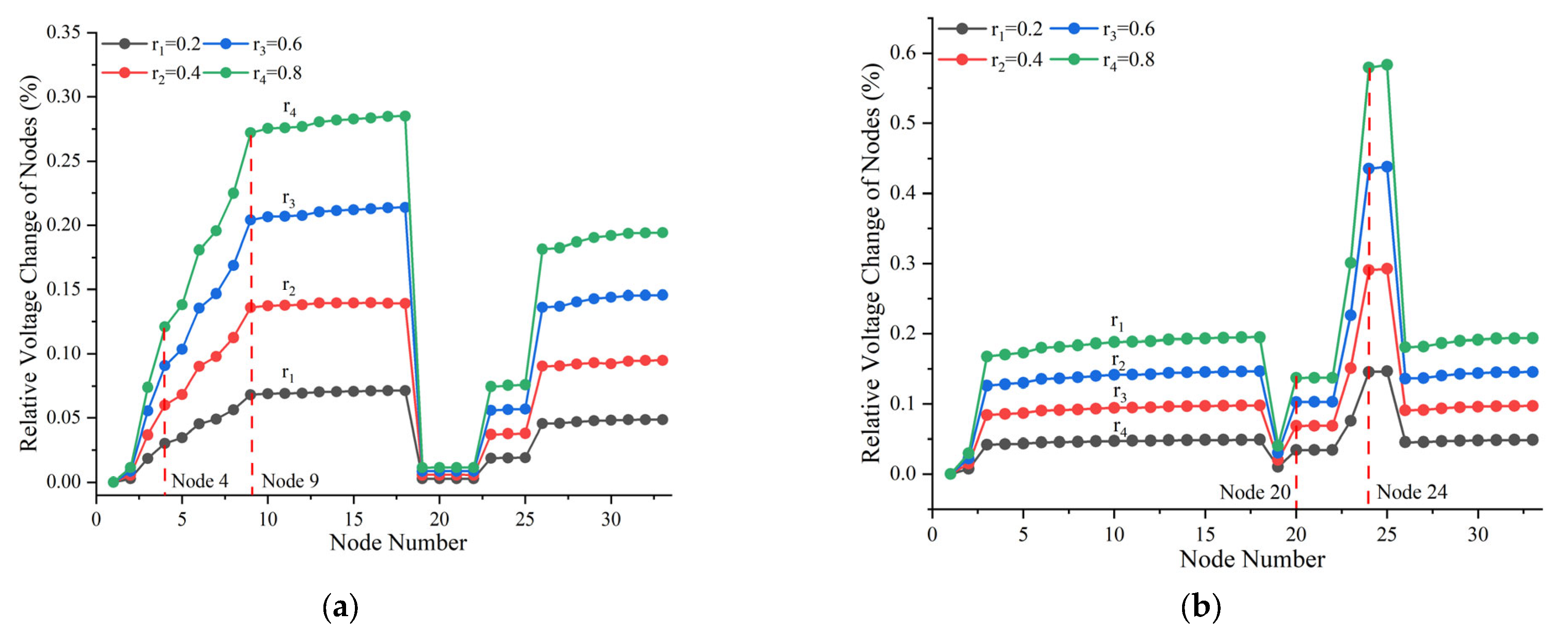
Figure 5a,b illustrate the spatial distribution of relative node voltage changes under multi-node anomalies in the IEEE-33 distribution network. In the trunk-feeder scenario (Figure 5a), voltage variation rates in the upstream region of anomalous nodes (nodes 1–9) increase with electrical distance from the source, peaking at nodes 4 and 9. Downstream branch nodes exhibit voltage changes comparable to their nearest anomalous node, while lateral branches (nodes 19–23, 23–25) follow the variations in their respective connection points on the main feeder. In the secondary branch scenario (Figure 5b), trunk feeder voltages remain stable (fluctuations <0.1%), whereas terminal branch nodes 20 and 24 experience significant voltage surges.

In these cases, each anomalous node induces abnormal currents in its upstream branches, which in turn generate ohmic voltage drops on the corresponding line impedances. Consequently, the upstream feeders of multiple anomalous nodes consistently exhibit a distance-dependent increase in voltage variation rate. Branch voltages are always constrained by the potentials of their connection points to the main feeder. Regardless of whether theft occurs on a single-node or multi-node system, voltage disturbances on branch feeders remain synchronized with their main feeder connection points—an inherent property determined by electrical connectivity. Both single-node anomalies (Figure 4d, node 25) and multi-node anomalies (Figure 5b, nodes 20 and 24) exhibit elevated voltage change rates at terminal nodes, indicating the relative instability of electrical node voltages at these locations.

Simulation experiments indicate that each anomalous node precipitates incremental voltage change rates in subsequent branch nodes. When the anomalous nodes are located in close proximity, the voltage fluctuations rise sharply. This reveals that the spatial distribution of anomalous nodes directly influences electrical parameter fluctuations in the distribution network.

(2)

Branch Current Variation under Multi-Node Anomalies

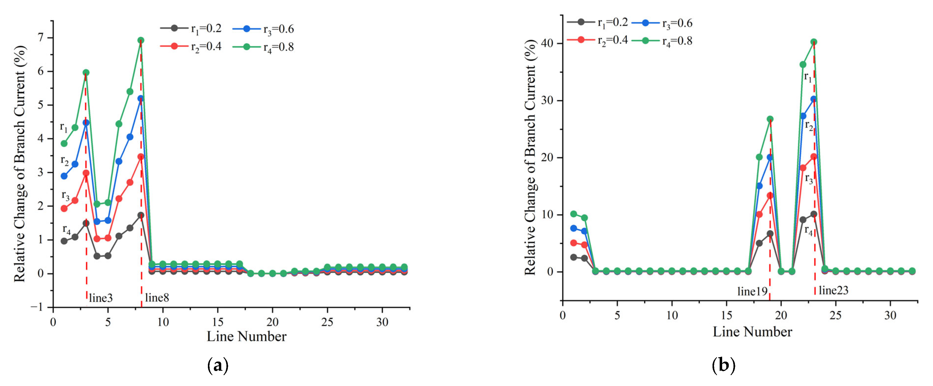
Figure 6a,b depict relative branch current variations under multi-node anomalies. In the trunk-feeder theft scenario (Figure 6a), upstream branches of anomalous nodes (Line 1–2 and Line 5–7) exhibit gradually increasing currents, peaking at terminal branches connected to anomalous nodes (Line 3 and Line 8). Subsequent branches (Line 9–18) and lateral branches (Line 18–24) show negligible changes.

In the branch feeder theft scenario (Figure 6b), currents in branches directly connected to anomalous nodes (Line18–19 and Line22–23) also increase progressively, reaching their maximum at the anomalous nodes. Due to shorter paths and higher branch resistances, current variations in lateral feeders are more pronounced than in the trunk feeder.

Overall, in multi-node theft conditions, abnormal currents originating from each anomalous node propagate upstream toward the source, causing incremental increases in upstream branch currents and peaking at the terminal branches where theft occurs. This trend is consistent with single-node theft scenarios. Furthermore, because of their shorter paths and higher resistances, branch feeders exhibit more substantial current fluctuations than trunk feeders under identical theft levels.

(3)

Branch Power Loss Variation under Multi-Node Anomalies

Multi-node theft scenarios are simulated at trunk nodes 4 and 6 and branch nodes 20 and 24.

Table 7. Relative Variation in Branch Power Loss under Multi-Node Anomaly (%).

No.	Electricity Theft at Nodes 4 and 9				Electricity Theft at Nodes 20 and 24
	r1 = 0.2	r2 = 0.4	r3 = 0.6	r4 = 0.8	r1 = 0.2	r2 = 0.4	r3 = 0.6	r4 = 0.8
Line1	1.921	3.821	5.702	7.562	5.034	9.923	14.669	19.273
Line2	2.156	4.286	6.391	8.471	4.704	9.28	13.728	18.049
Line3	2.964	5.88	8.748	11.569	0.095	0.189	0.283	0.376
Line4	1.030	2.053	3.068	4.077	0.095	0.19	0.284	0.378
Line5	1.053	2.098	3.136	4.166	0.095	0.19	0.285	0.379
Line6	2.211	4.394	6.548	8.675	0.095	0.189	0.282	0.376
Line7	2.687	5.333	7.939	10.504	0.095	0.19	0.285	0.379
Line8	3.441	6.817	10.127	13.372	0.096	0.192	0.288	0.383
Line9	0.141	0.281	0.421	0.56	0.097	0.193	0.288	0.384
Line10	0.141	0.282	0.422	0.561	0.097	0.193	0.289	0.384
Line11	0.141	0.282	0.422	0.562	0.097	0.193	0.290	0.385
Line12	0.142	0.283	0.424	0.564	0.097	0.194	0.290	0.386
Line13	0.142	0.283	0.424	0.565	0.097	0.194	0.291	0.387
Line14	0.142	0.284	0.425	0.566	0.098	0.195	0.291	0.388
Line15	0.142	0.284	0.426	0.567	0.098	0.195	0.292	0.388
Line16	0.143	0.285	0.426	0.568	0.098	0.195	0.292	0.389
Line17	0.143	0.285	0.427	0.568	0.098	0.195	0.292	0.389
Line18	0.006	0.011	0.017	0.023	9.804	19.096	27.878	36.149
Line19	0.006	0.011	0.017	0.023	12.94	24.976	36.11	46.343
Line20	0.006	0.011	0.017	0.023	0.069	0.137	0.206	0.274
Line21	0.006	0.011	0.017	0.023	0.069	0.137	0.206	0.274
Line22	0.038	0.076	0.113	0.151	17.414	33.119	47.131	59.464
Line23	0.038	0.076	0.113	0.151	19.205	36.317	51.355	64.335
Line24	0.038	0.076	0.114	0.152	0.292	0.583	0.871	1.157
Line25	0.096	0.191	0.287	0.382	0.096	0.191	0.286	0.381
Line26	0.096	0.192	0.287	0.383	0.096	0.192	0.287	0.382
Line27	0.096	0.192	0.288	0.384	0.096	0.192	0.288	0.383
Line28	0.096	0.193	0.288	0.384	0.096	0.192	0.288	0.383
Line29	0.097	0.193	0.289	0.385	0.097	0.193	0.288	0.384
Line30	0.097	0.194	0.290	0.385	0.097	0.193	0.288	0.384
Line31	0.097	0.194	0.291	0.385	0.097	0.194	0.290	0.386
Line32	0.097	0.194	0.291	0.385	0.097	0.194	0.290	0.386

summarizes relative branch power loss variations. Using the source side as a reference, it is observed that branches adjacent to anomalous nodes exhibit significantly higher increases in power loss compared with other branches, and the magnitude of variation is strongly correlated with the topological location of the anomalous nodes. This finding suggests that branch power loss can serve as an effective localization indicator, where the analysis of loss gradients enables identification of anomalous nodes within the network.

3. Spatiotemporal Feature Fusion-Based Improved DBSCAN for Anomalous Nodes Detection

Power flow analysis results show that, under normal operating conditions and electricity theft scenarios, the distribution network exhibits significantly different patterns in the distribution of electrical parameters. Abnormal consumption at nodes introduces load disturbances that propagate through the network, with their magnitude strongly dependent on nodes’ topological positions. To enable unsupervised detection of anomalous nodes, it is essential to construct a recognition model that integrates both spatial and temporal features. From the spatial perspective, the connectivity among nodes must be exploited, while from the temporal perspective, the dynamic characteristics of voltage magnitudes, branch current phases, and complex power fluctuations must be captured.

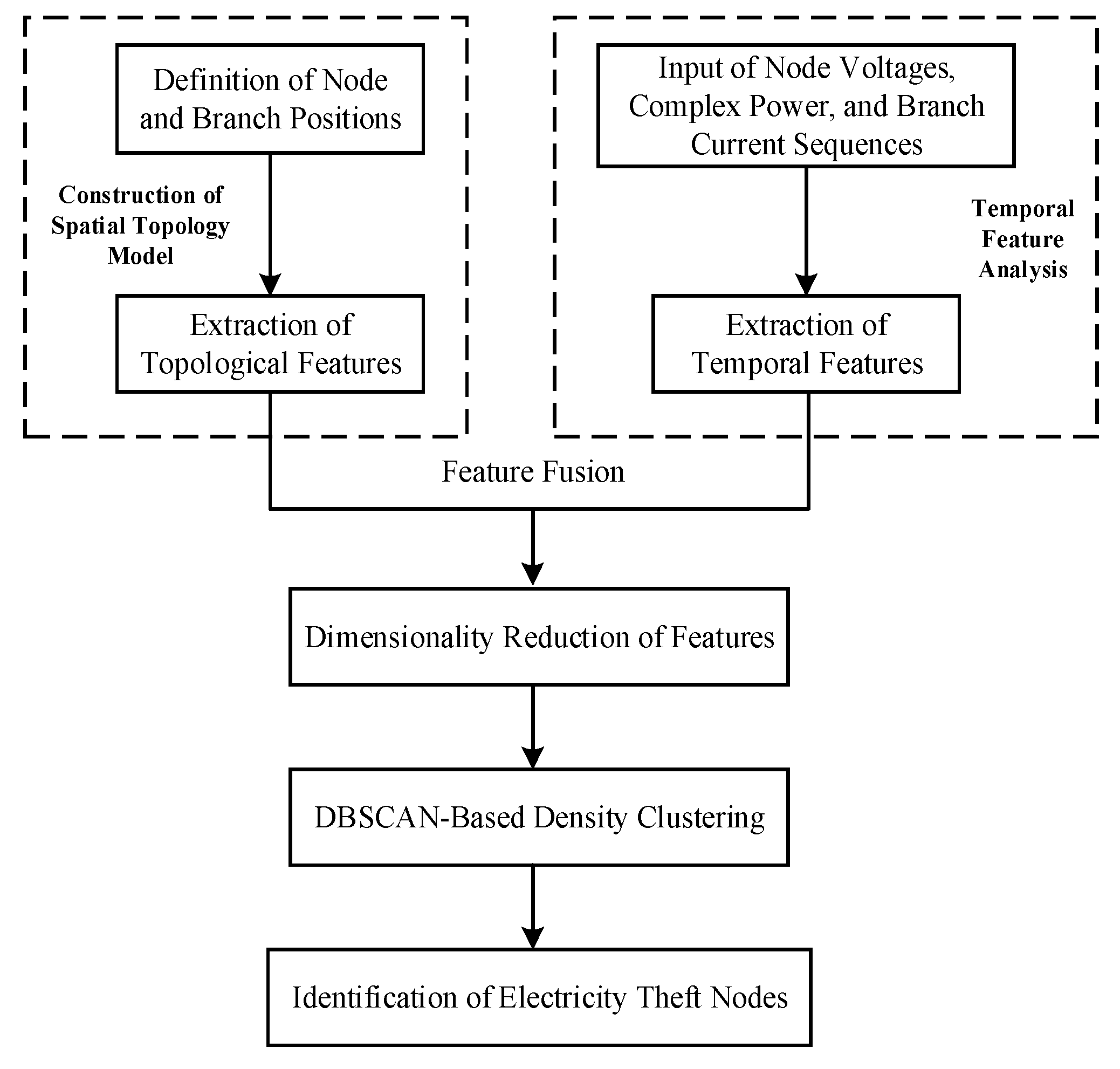
This paper proposes an improved DBSCAN-based method for electricity theft detection using spatiotemporal fusion features, with operational data from distribution feeders as the foundation. The overall procedure is illustrated in Figure 7. The method comprises three steps: first, establishing a nodal spatial topology model based on grid connectivity relations and analyzing the time-series variation features of parameters such as voltage and current; second, integrating spatial and temporal features and applying PCA for dimensionality reduction; finally, employing DBSCAN density-based clustering to automatically identify anomalous nodes.

3.1. Extraction of Topological Features and Load Data Features

The 10 kV distribution feeder is characterized by a tree-like topology, where node positions are determined by their physical connectivity. Specifically, the low-voltage side of the 35 kV/11 kV or 110 kV/11 kV transformer is defined as the root node, while the high-voltage side of the 11 kV/0.4 kV transformer serves as the leaf nodes. The adjacency matrix $A\in {\{0,1\}}^{\mathit{N}\times \mathit{N}}$ is employed to represent the connectivity among nodes, where $A_{ij}=1$ indicates that node $i$ is directly connected to node $j$. Based on this relationship, five categories of spatial network features are extracted, with their calculation methods summarized in

Table 8. Spatial Network Characteristic Parameters and Their Calculation Methods.

No.	Topological Feature	Calculation Method
1	Node Closeness Centrality	$C_{close}(i)={\displaystyle \frac{N-1}{{\displaystyle {\sum }_{j\ne i}d(i,j)}}}$
2	Node Betweenness Centrality	$C_{btw}(i)={\displaystyle {\sum }_{s\ne i\ne t}\frac{{\delta }_{st(i)}}{{\delta }_{st}}}$
3	Node Hierarchical Depth	$D(i)=l(i)$
4	Neighbor Connectivity Density	$p(i)={\displaystyle \frac{k_i}{k_{\max }}}$
5	Electrical Coupling Strength	$E(i)={\displaystyle \frac{1}{{\mathit{Z}}_{avg}(i)}}\hspace{1em}$${\mathit{Z}}_{\mathrm{avg}}(i)={\displaystyle \frac{1}{k_i}}{\displaystyle \sum _{j\in \mathcal{N}(i)}{\mathit{Z}}_{ij}}$

Here, $N$ denotes the total number of nodes; $d(i,j)$ is the shortest path length between nodes $i$ and $j$; ${\delta }_{st}$ is the total number of shortest paths between nodes $s$ and $t$; ${\delta }_{st(i)}$ is the number of shortest paths passing through node $i$; $l(i)$ represents the shortest path length from the root node to node $i$; $k_i$ and $k_{\max }$ denote the actual and maximum possible number of neighbors, respectively; $Z_{ij}$ is the impedance magnitude of the branch between node $i$ and its neighbor; and $N(i)$ is the neighbor set of node $i$.

.

The listed spatial network features characterize structural properties of distribution network nodes from different dimensions. Node closeness centrality measures the extent to which a node is close to the network core; anomalous nodes are typically located at the periphery but can induce deviations in central node parameters. Node betweenness centrality reflects the bridging role of a node, where anomalies on critical paths can exert wider influence. Node hierarchical depth describes the vertical position within the tree structure. Neighbor connectivity density reveals local sparsity, where low-density regions are more likely to conceal anomalies. Electrical coupling strength captures electrical correlations with adjacent nodes; theft behaviors cause observable fluctuations in the parameters of neighboring nodes.

Electrical parameters within the distribution transformer area display seasonal cyclic fluctuation characteristics over time. Based on annual time-series data of node voltages, branch currents, and complex power, load usage patterns at both the feeder and node level can be identified, while theft behaviors lead to significant abnormal deviations. For implementation, annual data are divided into monthly windows, from which temporal features of voltage, current, and power at each node are extracted, thereby constructing a load behavior analysis framework covering the annual cycle. With monthly data as the analysis unit, the extracted temporal electrical features are summarized in

Table 9. Summary of Extracted Temporal Electrical Features.

No.	Feature Name	Calculation Method	No.	Feature Name	Calculation Method
1	Monthly Average Voltage	${\overline{V}}_m={\displaystyle \frac{1}{T}}{\displaystyle {\sum }_{t=1}^T{V}_t}$	9	Current Jump Frequency	$\mathrm{Count}\left({\displaystyle \frac{\left|I_{t+1}-I_t\right|}{{\overline{I}}_m}}>0.3\right)$
2	Voltage Fluctuation Index	${\sigma }_V=\sqrt{{\displaystyle \frac{1}{N}}{\displaystyle \sum _{t=1}^T{(V_t-{\overline{V}}_m)}^2}}$	10	Monthly Active Power Integral	$E_P={\displaystyle \sum _{t=1}^N{P}_t}\Delta t$
3	Voltage Skewness	$S_V={\displaystyle \frac{\frac{1}{T}{\displaystyle {\sum }_{t-1}^T{(V_t-{\overline{V}}_m)}^3}}{{\sigma }_V^3}}$	11	Monthly Reactive Power Integral	$E_Q={\displaystyle \sum _{t=1}^N{Q}_t}\Delta t$
4	Weekly Fluctuation Rate	${\sigma }_{V,w}={\displaystyle \frac{1}{4}}{\displaystyle \sum _{k=1}^4{\sigma }_{V,k}}$	12	Mean Power Factor	${\mathrm{PF}}_m={\displaystyle \frac{1}{N}}{\displaystyle \sum _{t=1}^N\frac{P_t}{\sqrt{P_t^2+Q_t^2}}}$
5	Mean Daily Peak-to-Valley Voltage	$\Delta V_{day}={\displaystyle \frac{1}{D}}{\displaystyle \sum _{d=1}^D\left(\max (V_d)-\min (V_d)\right)}$	13	Power–Current Covariance	$\mathrm{Cov}(P,I)={\displaystyle \frac{1}{N}}{\displaystyle \sum _{t=1}^N(P_t-{\overline{P}}_m)}(I_t-{\overline{I}}_m)$
6	Voltage Jump Frequency	$\mathrm{Count}\left(\left|V_t-{\overline{V}}_m\right|>3{\delta }_V\right)$	14	Power Output per Unit Current	$\eta ={\displaystyle \frac{{\overline{P}}_m}{{\overline{I}}_m}}$
7	Monthly Average Current	${\overline{I}}_m={\displaystyle \frac{1}{T}}{\displaystyle {\sum }_{t=1}^T{I}_t}$	15	Voltage–Current Correlation Coefficient	${\rho }_{V,I}={\displaystyle \frac{\mathrm{Cov}(V_t,I_t)}{{\sigma }_V{\sigma }_I}}$
8	Peak-to-Valley Current Difference	$\Delta I_{\max -\min }=\max (I_t)-\min (I_t)$	16	Power-Time Peak-Valley Synchronization	$\mathrm{Sync}={\displaystyle \frac{\mathrm{Count}\left(\arg \max (P_d)=\arg \max (V_d)\right)}{D}}$

Here, $T$ is the number of sampling points in the month; $\Delta t$ is the sampling interval; $V_t$ is the voltage at sampling instant $t$; ${\overline{V}}_m$ is the monthly average voltage; $V_d$ is the voltage sequence of day $d$; ${\sigma }_V$ is the voltage standard deviation; ${\sigma }_{V,k}$ is the standard deviation of weekly voltage; ${\delta }_V$ denotes the voltage fluctuation index; $I_t$ is the current at sampling instant $t$; ${\overline{I}}_m$ is the monthly average current; $P_t$ and $Q_t$ are the active and reactive power at sampling instant $t$; ${\overline{P}}_m$ is the monthly average active power; ${\sigma }_I$ is the current standard deviation; $\arg \max (P_d)$ and $\arg \max (V_d)$ represent the peak and valley instants of power and voltage, respectively.

.

Among the electricity consumption features, Features 1–6 are derived from voltage data, Features 7–9 are extracted from current data, Features 10–12 are generated from power data, and Features 13–16 are obtained by combining the relationships among voltage, current, and power. These features capture regularities, periodicity, and parameter correlations, thereby simplifying computation while retaining critical information, and enabling a comprehensive analysis of the electricity consumption patterns of each node.

3.2. Feature Dimensionality Reduction

The feature set constructed based on the spatiotemporal feature extraction method consists of T months of multidimensional monitoring data per sample (with D feature parameters per month), forming a high-dimensional multivariate time-series feature set of size T × D. Direct application of unsupervised clustering algorithms to such high-dimensional data can be severely affected by the “curse of dimensionality”, which may distort Euclidean distance calculations between samples, leading to biased cluster partitioning and misclassification of noise points. To address this, Principal Component Analysis (PCA) is employed to perform global dimensionality reduction, extracting principal component vectors that account for over 90% of the cumulative variance. This approach compresses the feature space while retaining the major variance information of the original data [29].

Initially, the feature matrix of the i-th node $X_i\in {ℝ}^{T\times D}$ is flattened as:

$$x_i=\mathrm{vec}(X_i)={\left[x_{i,1}^{(1)},x_{i,2}^{(1)},\dots ,x_{i,D}^{(T)}\right]}^{\top }\in {ℝ}^{T\cdot D},$$

(2)

where $x_{i,1}$ to $x_{i,5}$ denotes spatial features, and $x_{i,6}$ to $x_{i,21}$ denotes temporal features.

To avoid the influence of differing units across dimensions, Z-score standardization is applied to each feature:

$$z_{i,k}={\displaystyle \frac{z_{i,k}-{\mu }_k}{{\sigma }_k}},\hspace{1em}k=1,2,\dots ,21,$$

(3)

where ${\mu }_k$ and ${\sigma }_k$ are the mean and standard deviation of the k-th feature across all nodes in the distribution network.

The standardized data matrix $Z\in {ℝ}^{N\times (T\cdot D)}$ is then computed as:

$$C={\displaystyle \frac{1}{N-1}}{Z}^{\top }Z$$

(4)

The covariance matrix $C$ is decomposed by eigenvalue decomposition:

$$C=V\Lambda V^{\top }$$

(5)

where $\Lambda =\mathrm{diag}({\lambda }_1,{\lambda }_2,\dots ,{\lambda }_{T\cdot D})$ is the diagonal matrix of eigenvalues, and $\mathrm{V}=[{\mathrm{v}}_1,{\mathrm{v}}_1,\dots ,{\mathrm{v}}_{T\cdot D}]$ is the matrix of eigenvectors.

The variance contribution rate for each feature is calculated as:

$${\mathrm{CR}}_j={\lambda }_j/{\displaystyle \sum _{i=1}^{T\cdot D}{\lambda }_i}$$

(6)

The first k principal components are selected such that the cumulative variance contribution rate meets or exceeds the threshold, and the data is projected onto these components for dimensionality reduction:

$${\mathrm{F}}_{\mathrm{PCA}}{=\mathrm{ZV}}_{[:,1:\mathrm{k}]}=[F_1,F_2,\dots ,F_k]\in {ℝ}^{\mathrm{N}\cdot \mathrm{k}}$$

(7)

3.3. Anomalous Node Identification Based on DBSCAN

Density-Based Spatial Clustering of Applications with Noise (DBSCAN) is a density-based unsupervised clustering algorithm. Its core principle is to partition high-density regions into clusters by defining a neighborhood density threshold $ϵ$ and a minimum number of neighbors $MinPts$, while sparsely distributed outliers are identified as noise. Compared with traditional clustering methods, DBSCAN does not require a predefined number of clusters and is highly adaptable to arbitrarily shaped data distributions, making it particularly suitable for detecting anomalous nodes with irregular and unknown spatial distribution in electricity theft scenarios [30].

Based on the number of nodes in the distribution area and empirical experience, $MinPts$ is specified. The Euclidean distance from each node to its $MinPts$-th nearest neighbor is calculated and denoted as the $k$-distance (8):

$$d(F_i,F_j)=\sqrt{{\displaystyle \sum _{k=1}^D{\left(f_{ik}-f_{jk}\right)}^2}},$$

(8)

All nodes’ $k$-distances are sorted in ascending order, selecting the distance of maximal curvature as $ϵ$:

$$ϵ=\arg {\max }_x\left|{\displaystyle \frac{d^{2}k(x)}{d{x}^2}}\right|,$$

(9)

For each node $F_i$, its $ϵ$-neighborhood is defined as the ensemble of all samples $F_i$ with Euclidean distances not exceeding $ϵ$:

$$N_{ϵ}(F_i)=\left\{F_j\in D|d(F_i,F_j)\le ϵ\right\},$$

(10)

If the number of samples within the neighborhood $N_{ϵ}(F_i)$ of node $F_i$ is not less than $MinPts$, then $F_i$ is defined as a core point. If node $F_j\in N_{ϵ}(F_i)$ but does not itself satisfy the core point condition, it is designated as a border point. If node $F_k\in N_{ϵ}(F_i)$ and $F_i$ is a core point, then $F_k$ is said to be directly density-reachable from $F_i$. Furthermore, if there exists a chain of nodes $F_i\to F_j\to F_k\to \cdots \to F_z$, then the node $F_z$ is considered density-reachable from $F_i$.

Starting from an unvisited core node, all density-reachable nodes are recursively merged into a single cluster. When no new nodes can be added, the expansion of that cluster ends. After all clusters are formed, nodes not assigned to any cluster are identified as noise points, which are directly regarded as anomalous nodes.

To evaluate the clustering performance in identifying anomalous nodes, three mainstream metrics are employed: Silhouette Coefficient, Calinski–Harabasz Index, and Davies–Bouldin Index:

• Silhouette Coefficient evaluates clustering quality by comparing the average intra-cluster distance with the nearest-cluster distance. Its value ranges from −1 to 1, with values closer to 1 indicating better cluster structure.
• Calinski–Harabasz Index is based on the ratio of between-cluster variance to within-cluster variance, with higher values indicating better inter-cluster separation and intra-cluster compactness.
• Davies–Bouldin Index calculates the mean ratio of intra-cluster compactness to inter-cluster separation; lower values indicate superior clustering performance.

Table 10. Comparison of Clustering Performance.

Evaluation Metric	K-Means Results	DBSCAN Results
Silhouette Coefficient	0.32	0.68
Calinski–Harabasz Index	152.7	286.4
Davies–Bouldin Index	1.85	0.62

compares K-means and DBSCAN clustering results across these metrics.

DBSCAN significantly outperforms K-means: the Silhouette Coefficient increases to 0.68, the Calinski–Harabasz Index reaches 286.4, and the Davies–Bouldin Index decreases to 0.62. These results confirm that DBSCAN is effective in identifying complex and sparsely distributed anomalous nodes. Therefore, DBSCAN is selected as the unsupervised method for detecting anomalous nodes in the distribution network.

4. Case Study of Anomalous Node Identification in a Distribution Feeder

4.1. Feeder Topology and Two-Anomalous-Node Scenario

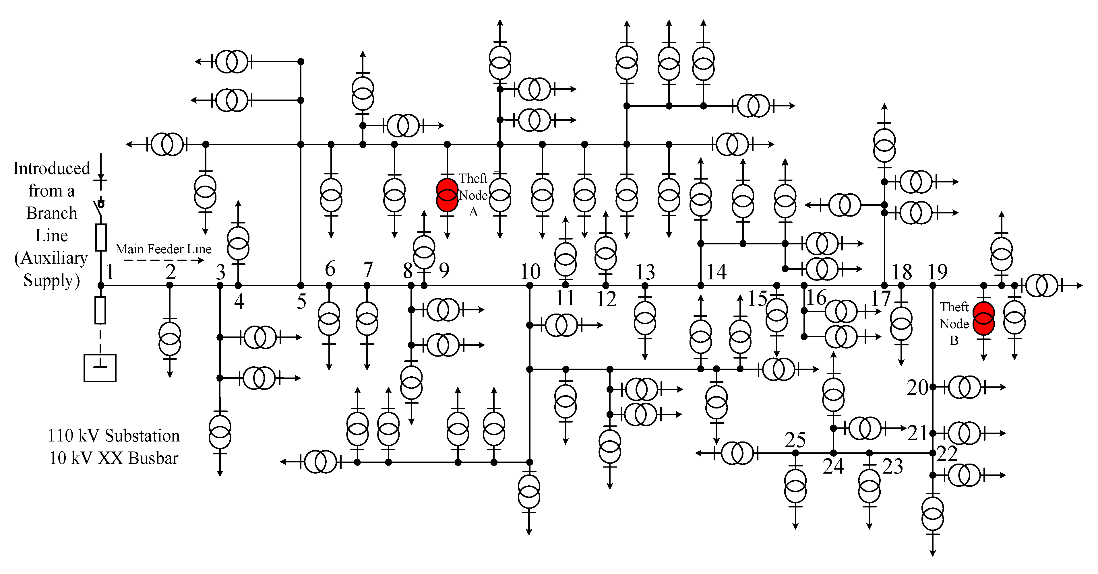
A 10 kV busbar distribution network of a substation is selected as the application case for algorithm validation, with its topology illustrated in Figure 8. The network comprises 76 public transformers, with a total line length of 98.86 km and a rated capacity of 8085 kVA.

Based on one-year operational data of node voltages, nodal complex power, and branch currents, 5–10% of the nodes were randomly selected as anomalous nodes. Corresponding electrical parameters for these nodes were generated, and the resulting theft disturbance data were combined with historical normal data at a 10% anomaly sample ratio to construct a hybrid validation dataset. This dataset strikes a balance between realism and controllability, providing a reliable benchmark for evaluating the proposed anomalous nodes identification algorithm.

To demonstrate the effectiveness of the proposed method, a two-nodes exhibiting anomalous load behavior scenario is implemented. Two representative anomalous nodes, A and B, are marked in red in Figure 8, and all subsequent experiments and analyses are conducted under this scenario.

4.2. Node Feature Analysis

Feature extraction was performed using a monthly sliding window.

Table 11. Characteristic Values and Z-Score Standardized Values of Nodes under Normal Operating Conditions (January).

No.	Feature	Node A Value	Z-Score	Node B Value	Z-Score
1	Node Closeness Centrality	0.081	−0.32	0.078	−0.49
2	Node Betweenness Centrality	650	0.49	146	−0.55
3	Node Hierarchical Depth	9	−0.63	19	1.12
4	Neighbor Connectivity Density	0.027	0.037	0.027	0.037
5	Electrical Coupling Strength	4.80%	−0.45	3.60%	−1.11
6	Monthly Average Voltage (kV)	10.51	0.35	10.36	0.05
7	Voltage Fluctuation Index	0.15%	0.55	0.12%	0.42
8	Voltage Skewness	0.03	0.12	0.08	0.42
9	Weekly Fluctuation Rate	0.25%	−1.02	0.18%	−1.31
10	Mean Daily Peak-to-Valley Voltage (kV)	0.18	−0.75	0.25	0.13
11	Voltage Jump Frequency	1/month	−1.22	3/month	0.25
12	Monthly Average Current (A)	480.3	1.25	85.6	−0.32
13	Peak-to-Valley Current Difference (A)	78.5	0.28	45.2	−0.35
14	Current Jump Frequency	2/month	−0.54	5/month	0.84
15	Monthly Active Power Integral (MWh)	1380	1.12	65.8	−0.31
16	Monthly Reactive Power Integral (MVarh)	320	0.85	12.3	−0.67
17	Mean Power Factor	0.90	0.41	0.85	−0.23
18	Power-Current Covariance	0.65	0.95	0.42	0.25
19	Power Output per Unit Current (kW/A)	0.33	0.15	0.25	−0.45
20	Voltage-Current Correlation Coefficient	0.87	0.91	0.82	−0.54
21	Power-Time Peak-Valley Synchronization	0.92	0.65	0.75	0.26

lists the spatiotemporal feature values and their Z-score normalization results for Nodes A and B in January under normal operating conditions.

From the spatial network features, node A’s closeness centrality (Z = −0.32) is slightly closer to the network center than node B (Z = −0.49), although neither qualifies as a core node. The difference in betweenness centrality (node A Z = 0.49; node B Z = −0.55) indicates that node A functions as a transmission hub, while node B is at the downstream end.

From the temporal electrical features, node A exhibits typical industrial load behavior, with a monthly average current of 480 A (Z = 1.25), electricity consumption of 1380 MWh (Z = 1.12), and a power factor of 0.90, indicating stable operation. In contrast, node B has a monthly average current of 85.6 A (Z = −0.32), electricity consumption of 65.8 MWh (Z = −0.31), and experiences five current jumps in the month (Z = 0.84), demonstrating intermittent residential load patterns. These distinct differences in spatial and temporal features confirm the identifiability of nodes with different load characteristics.

After theft occurs (node A: undercurrent type; node B: phase-shifting type), the spatial network features remain unchanged, as theft actions do not alter network connectivity. However, temporal electrical features show notable deviations. Figure 9 presents the Z-score variations (ΔZ) before and after theft, where ΔZ is defined as the post-theft Z minus the pre-theft Z.

Node A exhibits systematic negative shifts in monthly average current (ΔZ = −0.48), monthly active power integral (ΔZ = −0.42), and voltage-current correlation coefficient (ΔZ = −0.73), revealing current attenuation patterns. Node B shows declines in power-current covariance (ΔZ = −0.43), monthly active power integral (ΔZ = −0.29), and power factor (ΔZ = −0.87), while monthly reactive power integral increases (ΔZ = +1.82), indicating phase disturbance effects. Both theft types cause significant deviation from normal feature patterns, confirming the sensitivity of spatiotemporal features to theft disturbances.

4.3. Detection Results of the Unsupervised Clustering Method

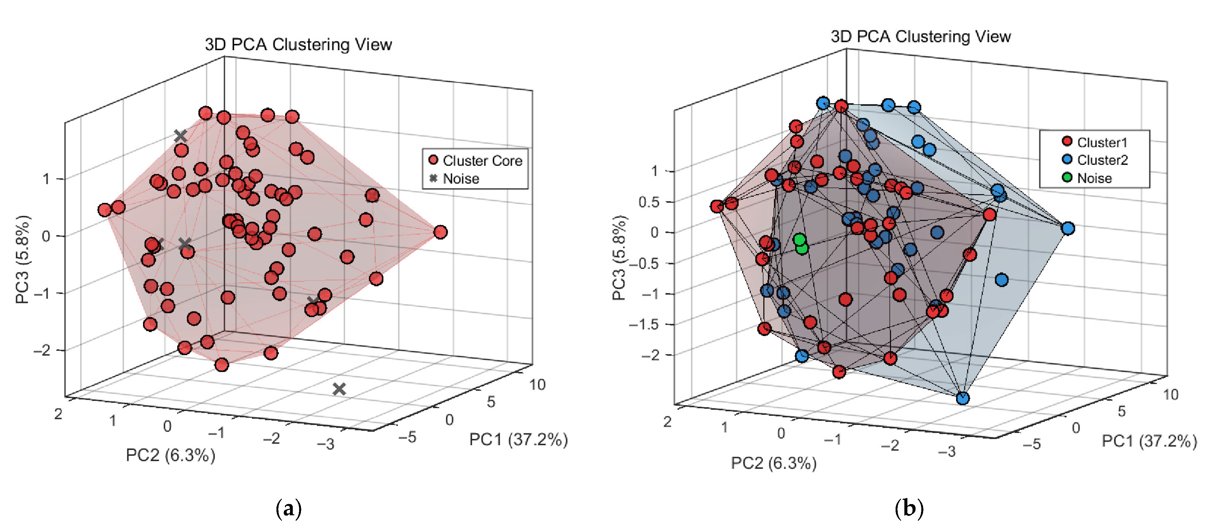
To evaluate the effectiveness of the proposed improved DBSCAN method in detecting anomalous nodes, experiments were conducted under the same feature extraction settings, with K-means clustering used for comparison. Figure 10a,b present 3D visualizations of the detected anomalous nodes, with X, Y, and Z axes corresponding to the top three principal components obtained via PCA.

As shown in Figure 10a, K-means identifies six noise points. Verification against feeder logs and tampering records reveals that five are normal nodes, and only one is an actual theft case, indicating a high false positive rate and reduced detection reliability. In contrast, Figure 10b demonstrates that the DBSCAN algorithm can adaptively identify clusters of varying densities, automatically separating the nodes into two user groups and accurately detecting two theft cases. By integrating feeder topology, the first group corresponds to residential areas (e.g., small community transformers and villages), and the second to industrial and commercial users (e.g., schools, hospitals, steel plants). The results demonstrate that the proposed DBSCAN method achieves higher detection accuracy and robustness than traditional K-means clustering.

4.4. Method Robustness and Quantitative Performance Evaluation

To further assess the robustness and effectiveness of the proposed approach, extended experiments were conducted on the 10 kV feeder case. Considering that theft typically occurs at low frequencies in real networks, anomaly ratios were set between 1% and 5%. Twenty combinations of dual-node theft scenarios were generated, forming 100 diverse validation samples that balance data volume and realistic variability.

Based on the benchmark feature set, six ablation experiments were conducted by removing different feature categories (Figure 11). The configurations were as follows: G0—All 21 spatiotemporal features; G1—Excluding spatial features; G2—Excluding voltage features; G3—Excluding current features; G4—Excluding power features; G5—Excluding cross-correlation features.

Under low-anomaly-rate conditions (1–5%), the full feature group (G0) achieved the best performance, with an accuracy of 90.7%, precision of 88.2%, recall of 87.5%, and an F1-score of 0.895.

Feature ablation experiments were conducted to quantify the contribution of different feature categories. As shown in Figure 11, excluding spatial (G1) or power features (G4) caused minor degradation, while removing current (G3) or cross-correlation features (G5) led to significant drops in performance, with F1-scores of 0.755 and 0.710, respectively. These results indicate that cross-correlation, current, and spatial features contribute most to model robustness, whereas voltage features have limited marginal impact.

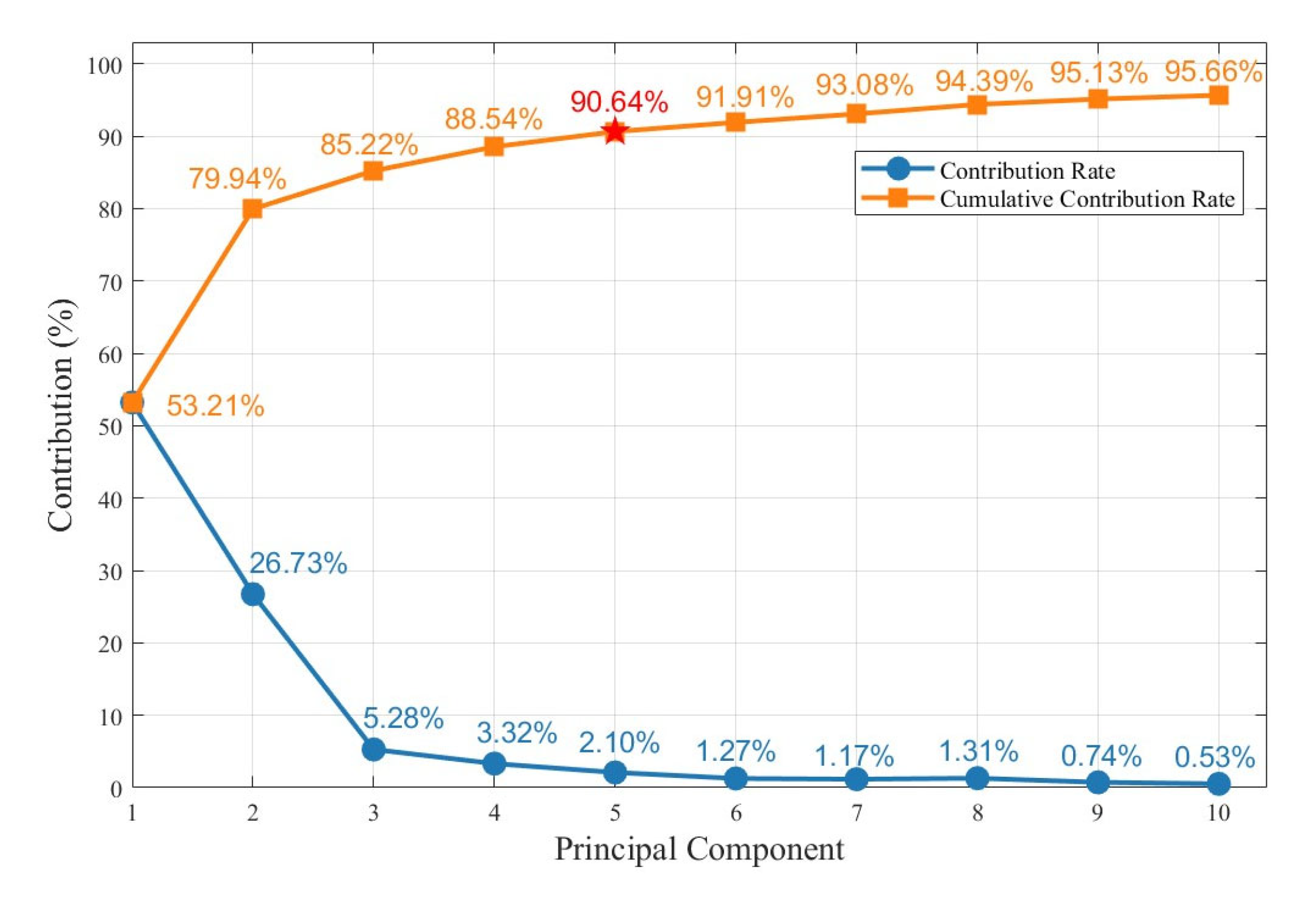
During PCA-based dimensionality reduction, component selection was determined by cumulative variance contribution. When the cumulative contribution exceeds 90%, the reduced representation can be considered to preserve the essential information of the original dataset. As shown in Figure 12, the first five principal components explain 53.21%, 26.73%, 5.28%, 3.32%, and 2.10% of the variance, respectively, with a cumulative contribution of 90.64%. Thus, five principal components are sufficient to capture the main variance structure while substantially reducing feature dimensionality. This ensures computational efficiency and supports reliable clustering-based identification of anomalous nodes.

4.5. Comparison with Supervised and Unsupervised Baselines

To evaluate overall performance, the proposed method was compared with K-means clustering and a supervised CNN model under low-anomaly-rate (1–5%) conditions. All methods used the same 21 standardized spatiotemporal features, and the CNN input was reshaped to match network requirements. The results are presented in

Table 12. Comparison of Detection Performance under Low Anomaly Rate (1–5%).

Method	Accuracy (%)	Anomaly Variability (%)	Noise Sensitivity (%)	Label Requirement
Proposed Method	90.72	±1.2	±2.15	None
CNN (Supervised)	92.31	±0.8	±1.53	High
K-means	84.84	±4.51	±6.32	None

.

In 100 low-anomaly (1–5%) distribution feeder samples, the supervised CNN model achieved slightly higher accuracy than the proposed improved DBSCAN method. However, CNN relies heavily on large amounts of labeled data, which are difficult to obtain in practice due to privacy constraints and the scarcity of confirmed theft labels in real power systems, making it unsuitable for large-scale deployment. Both the proposed method and K-means are unsupervised and require no labeled data. Nevertheless, the proposed approach outperforms K-means in terms of accuracy and stability, demonstrating stronger adaptability to real-world distribution networks where labeled data are limited.

5. Discussion

5.1. Practical Application Significance

The proposed improved DBSCAN-based unsupervised detection method demonstrates significant practical value in power distribution systems. Unlike supervised approaches that rely on extensive manual labeling, this method requires no prior labels. It can directly utilize multi-dimensional data collected by AMI to identify nodes exhibiting anomalous load behavior, effectively addressing the “label scarcity” issue commonly encountered in real-world scenarios. Since the algorithm depends only on basic measurements such as voltage, current, and power, it offers low deployment cost and strong scalability, enabling rapid implementation at the feeder or substation level. Experimental results confirm that the method maintains high accuracy and robustness under low anomaly rates (1–5%), making it an effective tool to support anti-theft operations in distribution networks.

5.2. Limitations

Although the proposed method achieves promising performance in terms of detection accuracy and practicality, several limitations remain. In real AMI systems, measurement data may suffer from noise interference, sampling loss, or drifting baselines, which can blur cluster boundaries and reduce detection accuracy. Moreover, when processing millions of user records or long time-series datasets, the computational complexity of density-based clustering may lead to reduced efficiency in large-scale environments.

5.3. Future Research Directions

Future work will focus on more realistic and complex distribution network scenarios. A closed-loop framework will be developed to integrate detection results with on-site verification. This will enable self-adaptive parameter tuning and continuous model optimization. In addition, parallel and distributed implementations of the algorithm will be explored to improve computational efficiency and scalability for large-scale power data applications. Moreover, the development of secondary post-clustering filters, such as those based on branch loss gradients or topological location, will be investigated to further mitigate potential false positives.

6. Conclusions

This study addresses the challenges of label scarcity, and complex feature interactions in distribution networks. An improved DBSCAN-based unsupervised detection method is proposed, integrating spatiotemporal features for identifying nodes exhibiting anomalous load behavior. The effectiveness of the proposed approach is verified through hybrid dataset experiments. The main conclusions are summarized as follows:

(1)

Based on the IEEE 33-bus benchmark distribution network, the disturbance patterns of voltage, current, and power loss under theft conditions were analyzed. Results indicate that the farther a theft node is from the power source, the stronger the propagated voltage and current disturbances along the feeder. The electrical distance is positively correlated with fluctuation amplitude. Meanwhile, branch loss peaks are localized near theft terminals and increase unidirectionally along the power flow path without back-propagation to downstream lines.

(2)

By exploring the correlation between theft disturbances and network topology, a comprehensive set of spatial, temporal, and cross-correlation features was constructed to represent node operating states. An improved DBSCAN clustering framework was developed based on these fused features.

(3)

Validation on hybrid datasets demonstrated that the proposed method achieved an accuracy of 90.7%, a recall of 87.5%, and an F1-score of 0.895, outperforming the traditional K-means algorithm and approaching the performance of supervised CNN models—without the need for labeled data.

(4)

The proposed method relies solely on basic electrical measurements such as voltage, current, and power, without requiring user labels or complex training. This ensures low deployment cost, strong scalability.

In summary, the improved DBSCAN-based method achieves high detection accuracy and robustness, offering a practical and scalable approach for electricity theft detection in distribution networks. Future work will focus on parallel optimization, and field feedback integration to further enhance the real-time performance and engineering applicability of the method.

References

1. Reddy Depuru, S.S.S.; Wang, L.; Devabhaktuni, V. Electricity theft: Overview, issues, prevention and a smart meter based approach to control theft. Energy Policy 2011, 39, 1007–1015. [Google Scholar] [CrossRef]
2. Jiang, R.; Lu, R.; Wang, Y.; Luo, J.; Shen, C.; Shen, X. Energy-theft detection issues for advanced metering infrastructure in smart grid. Tsinghua Sci. Technol. 2014, 19, 105–120. [Google Scholar] [CrossRef]
3. Massaferro, P.; Di Martino, J.M.; Fernández, A. Fraud detection in electric power distribution: An approach that maximizes the economic return. IEEE Trans. Power Syst. 2019, 35, 703–710. [Google Scholar] [CrossRef]
4. Esmael, A.A.; Da Silva, H.H.; Ji, T.; da Silva Torres, R. Non-technical loss detection in power grid using information retrieval approaches: A comparative study. IEEE Access 2021, 9, 40635–40648. [Google Scholar] [CrossRef]
5. Xia, X.; Xiao, Y.; Liang, W.; Cui, J. Detection methods in smart meters for electricity thefts: A survey. Proc. IEEE 2022, 110, 273–319. [Google Scholar] [CrossRef]
6. Muzumdar, A.; Modi, C.; Vyjayanthi, C. Designing a blockchain-enabled privacy-preserving energy theft detection system for smart grid neighborhood area network. Electr. Power Syst. Res. 2022, 207, 107884. [Google Scholar] [CrossRef]
7. Ahmad, T.; Chen, H.; Wang, J.; Guo, Y. Review of various modeling techniques for the detection of electricity theft in smart grid environment. Renew. Sustain. Energy Rev. 2018, 82, 2916–2933. [Google Scholar] [CrossRef]
8. Shahid, M.B.; Shahid, M.O.; Tariq, H.; Saleem, S. Design and development of an efficient power theft detection and prevention system through consumer load profiling. In Proceedings of the 2019 International Conference on Electrical, Communication, and Computer Engineering (ICECCE), Cox’s Bazar, Bangladesh, 7–9 February 2019; pp. 1–6. [Google Scholar]
9. Wang, Y.; Chen, Q.; Hong, T.; Kang, C. Review of smart meter data analytics: Applications, methodologies, and challenges. IEEE Trans. Smart Grid 2018, 10, 3125–3148. [Google Scholar] [CrossRef]
10. Messinis, G.M.; Hatziargyriou, N.D. Review of non-technical loss detection methods. Electr. Power Syst. Res. 2018, 158, 250–266. [Google Scholar] [CrossRef]
11. Luan, W.; Wang, G.; Yu, Y.; Lin, J.; Zhang, W.; Liu, Q. Energy theft detection via integrated distribution state estimation based on AMI and SCADA measurements. In Proceedings of the 2015 5th International Conference on Electric Utility Deregulation and Restructuring and Power Technologies (DRPT), Changsha, China, 26–29 November 2015; pp. 751–756. [Google Scholar]
12. Silva, L.G.d.O.; da Silva, A.A.; de Almeida-Filho, A.T. Allocation of power-quality monitors using the P-median to identify nontechnical losses. IEEE Trans. Power Deliv. 2016, 31, 2242–2249. [Google Scholar] [CrossRef]
13. Manito, A.R.; Bezerra, U.H.; Soares, T.M.; Vieira, J.P.; Nunes, M.V.; Tostes, M.E.; de Oliveira, R.C. Technical and non-technical losses calculation in distribution grids using a defined equivalent operational impedance. IET Gener. Transm. Distrib. 2019, 13, 1315–1323. [Google Scholar] [CrossRef]
14. Ferreira, T.S.D.; Trindade, F.C.; Vieira, J.C. Load flow-based method for nontechnical electrical loss detection and location in distribution systems using smart meters. IEEE Trans. Power Syst. 2020, 35, 3671–3681. [Google Scholar] [CrossRef]
15. Veeramani, P.; Aravindaguru, I.; Prathap, M.; Bhavesh, L.; Kamalesh, R.; Hassan, A.T. IOT Based Power Theft Detection For Transmission Lines. In Proceedings of the 2024 5th International Conference on Smart Electronics and Communication (ICOSEC), Tholurpatti, India, 18–20 September 2024; pp. 507–512. [Google Scholar]
16. Haq, E.U.; Pei, C.; Zhang, R.; Jianjun, H.; Ahmad, F. Electricity-theft detection for smart grid security using smart meter data: A deep-CNN based approach. Energy Rep. 2023, 9, 634–643. [Google Scholar] [CrossRef]
17. Bai, Y.; Sun, H.; Zhang, L.; Wu, H. Hybrid CNN-Transformer Network for Electricity Theft Detection in Smart Grids. Sensors 2023, 23, 8405. [Google Scholar] [CrossRef]
18. Fernandes, S.E.; Pereira, D.R.; Ramos, C.C.; Souza, A.N.; Gastaldello, D.S.; Papa, J.P. A probabilistic optimum-path forest classifier for non-technical losses detection. IEEE Trans. Smart Grid 2018, 10, 3226–3235. [Google Scholar] [CrossRef]
19. Ahir, R.K.; Chakraborty, B. Pattern-based and context-aware electricity theft detection in smart grid. Sustain. Energy Grids Netw. 2022, 32, 100833. [Google Scholar] [CrossRef]
20. Punmiya, R.; Choe, S. ToU Pricing-Based Dynamic Electricity Theft Detection in Smart Grid Using Gradient Boosting Classifier. Appl. Sci. 2021, 11, 401. [Google Scholar] [CrossRef]
21. Xia, X.; Lin, J.; Jia, Q.; Wang, X.; Ma, C.; Cui, J.; Liang, W. ETD-ConvLSTM: A Deep Learning Approach for Electricity Theft Detection in Smart Grids. IEEE Trans. Inf. Forensics Secur. 2023, 18, 2553–2568. [Google Scholar] [CrossRef]
22. Wu, Q.; Zhang, M.; Liao, L. Analysis of electricity stealing based on user electricity characteristics of electricity information collection system. Energy Rep. 2022, 8, 488–494. [Google Scholar] [CrossRef]
23. Peng, Y.; Yang, Y.; Xu, Y.; Xue, Y.; Song, R.; Kang, J.; Zhao, H. Electricity theft detection in AMI based on clustering and local outlier factor. IEEE Access 2021, 9, 107250–107259. [Google Scholar] [CrossRef]
24. Bondok, A.; Abdelsalam, O.; Badr, M.; Mahmoud, M.; Alsabaan, M.; Alsaqhan, M.; Ibrahem, M.I. Accurate Power Consumption Predictor and One-Class Electricity Theft Detector for Smart Grid “Change-and-Transmit” Advanced Metering Infrastructure. Appl. Sci. 2024, 14, 9308. [Google Scholar] [CrossRef]
25. Tian, L.; Xiang, M. Abnormal power consumption analysis based on density-based spatial clustering of applications with noise in power systems. Autom. Electr. Power Syst. 2017, 41, 64–70. [Google Scholar]
26. Zheng, K.; Wang, Y.; Chen, Q.; Li, Y. Electricity theft detecting based on density-clustering method. In Proceedings of the 2017 IEEE Innovative Smart Grid Technologies-Asia (ISGT-Asia), Auckland Central, New Zealand, 4–7 December 2017; pp. 1–6. [Google Scholar]
27. Dolatabadi, S.H.; Ghorbanian, M.; Siano, P.; Hatziargyriou, N.D. An enhanced IEEE 33 bus benchmark test system for distribution system studies. IEEE Trans. Power Syst. 2020, 36, 2565–2572. [Google Scholar] [CrossRef]
28. Baran, M.E.; Wu, F.F. Network reconfiguration in distribution systems for loss reduction and load balancing. IEEE Trans. Power Deliv. 2002, 4, 1401–1407. [Google Scholar] [CrossRef]
29. Gewers, F.L.; Ferreira, G.R.; Arruda, H.F.D.; Silva, F.N.; Comin, C.H.; Amancio, D.R.; Costa, L.d.F. Principal component analysis: A natural approach to data exploration. ACM Comput. Surv. 2021, 54, 1–34. [Google Scholar] [CrossRef]
30. Hahsler, M.; Piekenbrock, M.; Doran, D. dbscan: Fast density-based clustering with R. J. Stat. Softw. 2019, 91, 1–30. [Google Scholar] [CrossRef]
Figure 1. Radial Topological Structure of the IEEE 33-Node Distribution System.
Applsci 15 12028 g001
Figure 2. Voltage Distribution of Nodes in the IEEE-33 Distribution System. All voltage values are in kV. The color gradient from yellow to green to blue indicates the gradual voltage decrease along the feeder.
Applsci 15 12028 g002
Figure 3. Node Voltage Disturbance under a Single-Node Anomaly Scenario: (a) anomaly at node 4; (b) anomaly at node 6; (c) anomaly at node 14; (d) anomaly at node 24. The vertical red dashed line indicates the location of the anomalous node.
Applsci 15 12028 g003aApplsci 15 12028 g003b
Figure 4. Branch Current Disturbance under a Single-Node Anomaly Scenario: (a) anomaly at node 4; (b) anomaly at node 6; (c) anomaly at node 14; (d) anomaly at node 24. The vertical red dashed line indicates the branch containing the anomalous node.
Applsci 15 12028 g004aApplsci 15 12028 g004b
Figure 5. Node Voltage Disturbance under Multi-Node Anomaly Scenarios: (a) anomaly at nodes 4 and 9; (b) anomaly at nodes 20 and 24. The vertical red dashed line indicates the location of the anomalous node.
Applsci 15 12028 g005
Figure 6. Branch Current Disturbance under Multi-Node Anomaly Scenarios: (a) anomaly at nodes 4 and 9; (b) anomaly at nodes 20 and 24. The vertical red dashed line indicates the branch containing the anomalous node.
Applsci 15 12028 g006
Figure 7. Framework of Anomalous Node Detection in Distribution Networks.
Applsci 15 12028 g007
Figure 8. Distribution Topology Diagram of a 10 kV Busbar in a Substation.
Applsci 15 12028 g008
Figure 9. Standardized Scores of Node Features Before and After Electricity Theft.
Applsci 15 12028 g009
Figure 10. Three-dimensional PCA Clustering Visualization of the Case Study Area: (a) K-means clustering; (b) DBSCAN clustering.
Applsci 15 12028 g010
Figure 11. Robustness of the Proposed Method under Low Anomaly Rate Scenarios.
Applsci 15 12028 g011
Figure 12. Variance contribution rates and cumulative contribution rates of PCA components.
Applsci 15 12028 g012