Article

Landslide Susceptibility Mapping Using Remote Sensing Interpretation and a Blending-XGBoost-CNN Model

1
School of Architecture and Civil Engineering, Xi’an University of Science and Technology, Xi’an 710054, China
2
School of Civil Engineering and Geomatics, Shandong University of Technology, Zibo 255000, China
3
Geological Disaster Mitigation Department, Shandong Provincial Territorial Spatial Ecological Restoration Center, Jinan 250014, China
4
On-Site Inspection Section, Zibo Municipal Government Service Center, Zibo 255100, China
5
Boshan District Section, Zibo Bureau of Natural Resources, Zibo 255000, China
*
Author to whom correspondence should be addressed.
Appl. Sci. 2025, 15(22), 11969; https://doi.org/10.3390/app152211969
Submission received: 23 September 2025 / Revised: 31 October 2025 / Accepted: 3 November 2025 / Published: 11 November 2025

Abstract

The accuracy of historical landslide data is a key factor affecting the precision of landslide susceptibility mapping. The degree of conformity between mathematical models and disaster-prone environments cannot be predetermined, and the optimal model needs to be determined through comparative studies. In this paper, SBAS-InSAR and the object-oriented classification method were integrated to provide data for landslide susceptibility mapping: SBAS-InSAR was used to process Sentinel-1 images, while the object-oriented classification method was applied to interpret Landsat 8 images. Eleven hazard factors were selected for landslide susceptibility modeling, and the best-performing model was determined. The influences of single and multiple hazard factors on landslide susceptibility were analyzed using Geodetector. The results showed that 246 potential landslides were identified, with a total area of 0.427 km2 and a total volume of 2.161 × 10⁶ m3. The Blending-XGBoost-CNN model achieved the highest AUC and Precision, outperforming the XGBoost model and CNN model. The extreme high susceptible areas, high susceptible areas, moderate susceptible areas, minor susceptible areas and extreme minor susceptible areas accounted for 6.24% (91.4 km2), 15.07% (220.6 km2), 29.15% (426.8 km2), 30.58% (447.7 km2), and 18.96% (277.8 km2) of the total area, respectively. NDVI and gradient were key factors determining landslide occurrence. Elevation, slope aspect, distance from river, and land use also played significant roles in landslide occurrence. The contributions of TWI and lithology to landslide occurrence were relatively small, while those of plane curvature and distance from road were minimal. The interaction of hazard factors exhibited NE or BE relationships, not only increasing landslide risk but also potentially leading to more complex disaster patterns. This study can provide a theoretical basis for landslide prevention-oriented land use planning.

1. Introduction

A landslide is a natural phenomenon where rock and soil slide downward, either as a whole or in fragments, along a weak surface (weak zone) and under the influence of gravity [1]. According to China’s National Bureau of Statistics, 5659 geological disasters occurred in 2022, resulting in over 140 casualties and economic losses of 1502.81 million yuan. Among these, landslides accounted for 3919 incidents, representing 69.25% of the total [2]. Landslide susceptibility mapping (LSM) calculates landslide occurrence probability and divides areas into different susceptibility levels. This helps to understand the status and development trends of landslides, providing a basis for formulating scientific and effective disaster mitigation policies [3,4].
The accuracy of historical landslide data is a key factor affecting the precision of LSM [5]. Interferometric Synthetic Aperture Radar (InSAR) exhibits excellent performance in surface deformation monitoring, particularly in complex terrain environments. InSAR can provide continuous and stable monitoring data, offering high practical value for landslide identification [6]. The Small Baseline Subset InSAR (SBAS-InSAR) constructs multiple small baseline subsets by setting spatiotemporal baseline thresholds for multiple master images. This not only optimizes the data processing workflow but also enables high-precision joint solutions for each small baseline subset, yielding accurate time-series deformation results [7]. The object-oriented classification method transforms the spatial, textural, and spectral information of high-resolution panchromatic and multispectral data into an object-oriented format. By analyzing spatial relationships and feature differences of complex ground objects, this method achieves landslide identification based on multidimensional information, overcoming the issue of pixel spectral value interference caused by low-resolution remote sensing images [8,9]. Qin et al. [10] proposed a new remote-sensing image object detection algorithm based on the Faster R-CNN algorithm; a data augmentation method was then applied to the landslide dataset to solve the problem of an insufficient number of landslide samples in the training set. Yan et al. [11] presented an evaluation and prediction method of the potential long-runout landslide through the integration of remote sensing interpretation, SBAS-InSAR, and Massflow numerical simulation. The results revealed that Sentinel-1 ascending data were more appropriate for monitoring the deformation characteristics of the Songrong landslide. Chandra and Vaidya [12] extracted the landslide hazard information from multiple data sources, i.e., satellite and unmanned aerial vehicle (UAV) images, using a single staged object detection model, i.e., YOLOv5, YOLOv6, YOLOv7, and YOLOv8. The data from distinct platforms were utilized to infer the synergies between them. Choi et al. [13] presented a case study approach to fully leverage a variety of multi-source remote sensing technologies for analyzing the characteristics of a landslide. The chosen multi-source technologies encompassed digital photogrammetry using RGB and multi-spectral imagery, 3D point clouds acquired by light detection and ranging (LiDAR) mounted on UAV, and InSAR. Handwerger et al. [14] revisited the 2017 Mud Creek landslide in California using radar interferometry, pixel tracking, and elevation change measurements from satellite and airborne radar, LiDAR, and optical data. The results showed that pixel tracking of optical imagery captured the transition from slow motion to runaway acceleration starting one month before catastrophic failure—an acceleration undetected by satellite InSAR alone.
A single remote sensing interpretation method cannot guarantee the accuracy of historical landslide data [15]. The degree of conformity between mathematical models and disaster-prone environments cannot be predetermined, and the optimal model needs to be determined through comparative studies [16]. This study aimed to improve the identification accuracy of potential landslides by integrating SBAS-InSAR and the object-oriented classification method. The eXtreme Gradient Boosting (XGBoost) model, Convolutional Neural Networks (CNN) model and Blending-XGBoost-CNN model were employed for LSM, and the best model was selected. The landslide susceptible probabilities were divided into five levels: extreme minor susceptible, minor susceptible, moderate susceptible, high susceptible, and extreme high susceptible, and the landslide susceptible zoning maps were generated. The impacts of single and multiple hazard factors on landslide susceptibility were discussed based on Geodetector. The research flowchart is shown in Figure 1.

2. Study Area and Data

2.1. Overview of the Study Area

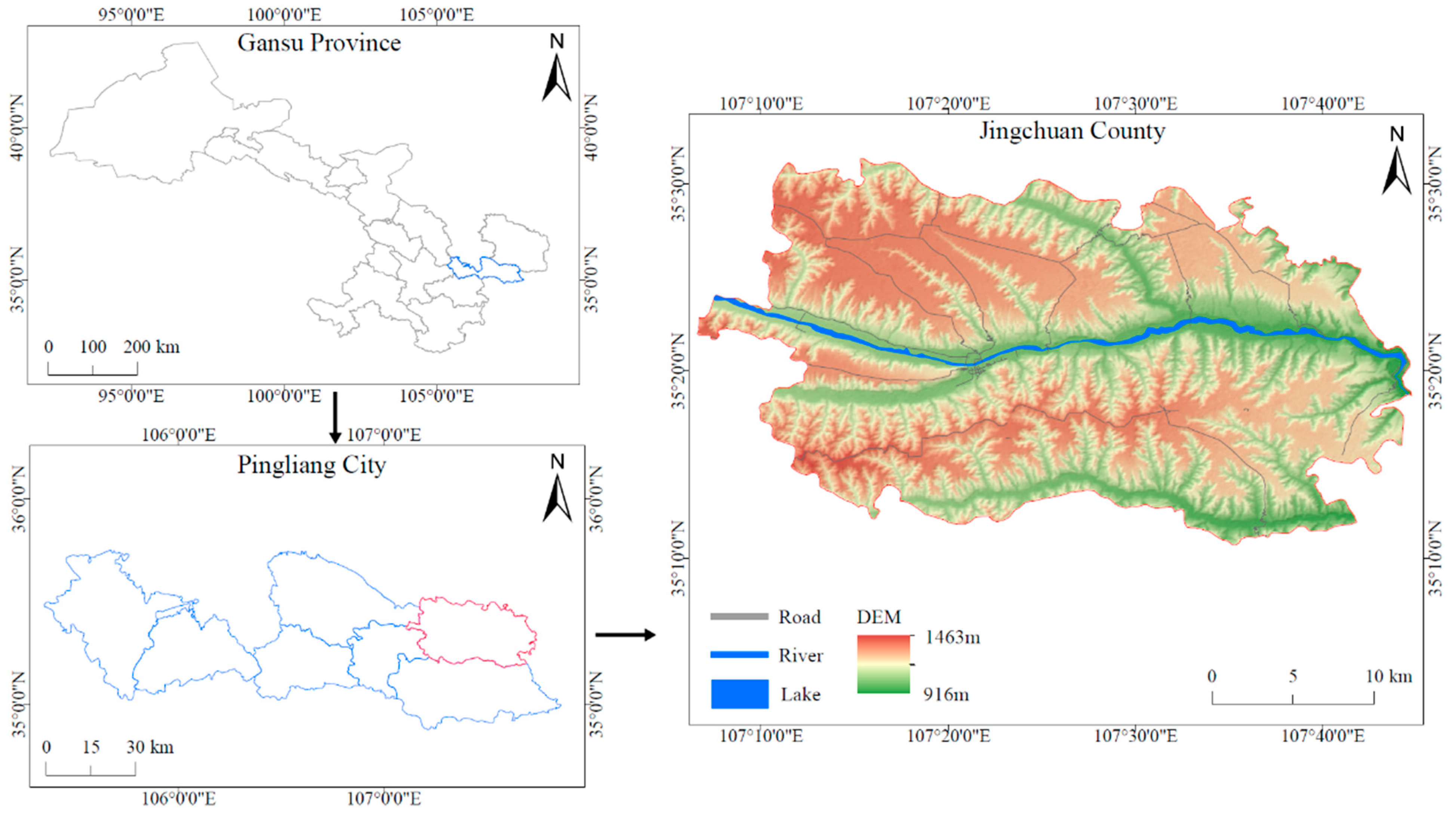
The study area is Jingchuan County, Pingliang City, Gansu Province, spanning from 107°15′ E to 107°45′ E, and 35°11′ N to 35°31′ N. It stretches 57 km from east to west and 36 km from north to south, covering an area of 1464 km2, as shown in Figure 2. The study area experiences a warm temperate semi-arid continental monsoon climate, with an average annual precipitation of 555 mm, of which over 65% occurs between June and September [17]. The terrain is higher in the west and lower in the east, with elevations ranging from 916 to 1463 m, and a cutting depth of 150–300 m. The study area is characterized by the Loess Plateau landforms of eastern Gansu, including loess hills and gully areas (63.4%), fragmented plateau areas (23.6%), river valleys and flatlands (9.4%), and other landforms (3.6%) [18].
The study area is situated on the southwestern edge of the Ordos Block. The exposed strata are primarily covered by Quaternary loess and fluvial deposits. The Cretaceous Zhidan Group’s Luohandong Formation and Jingchuan Formation strata are nearly horizontally exposed at the foot of river valley slopes and downstream gullies, with relatively simple stratigraphic structures [19]. The study area belongs to the Jing River Basin, a secondary tributary of the Yellow River. The main stream of the Jing River flows from west to east, with tributaries such as the Rui River and Hei River in the south, and the Hong River and Pu River in the north. Gullies are well-developed on both sides of the river valleys, with most gullies exposing descending springs that form perennial streams with flows of 1–5 L/s. Groundwater is classified into two types: Quaternary loose rock pore water and pre-Quaternary clastic rock fissure water [20].

2.2. Study Data and Sources

The data used in this study are shown in Table 1.

3. Identification of Potential Landslides in the Study Area

3.1. SBAS-InSAR

SBAS-InSAR reduces coherence differences by selecting subsets of SAR images with small baseline variations, thereby improving the accuracy and stability of deformation monitoring [21]. The Sentinel-1 satellite provides continuous SAR images [22]. Sixteen ascending orbit Sentinel-1A images were used in this study, covering a time range from 24 July 2022 to 16 November 2023, spanning 480 days.
(1) Preprocessing such as parameter setting, format conversion and region clipping were performed on the Sentinel-1A images using ENVI 5.6 [23].
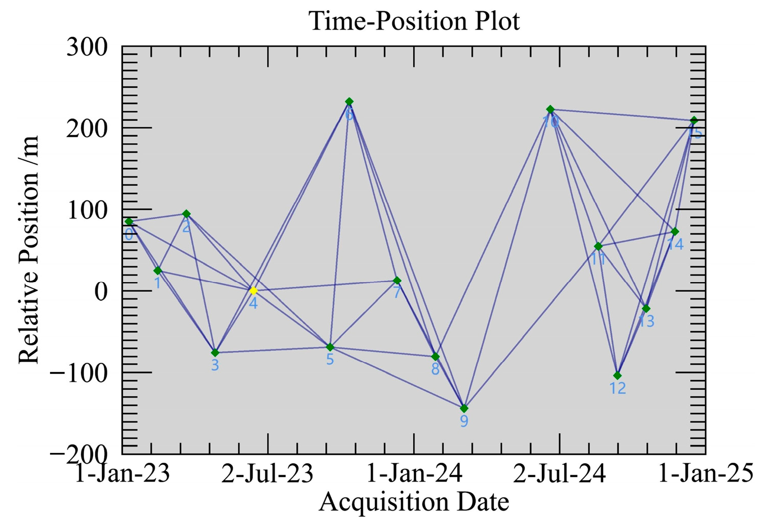
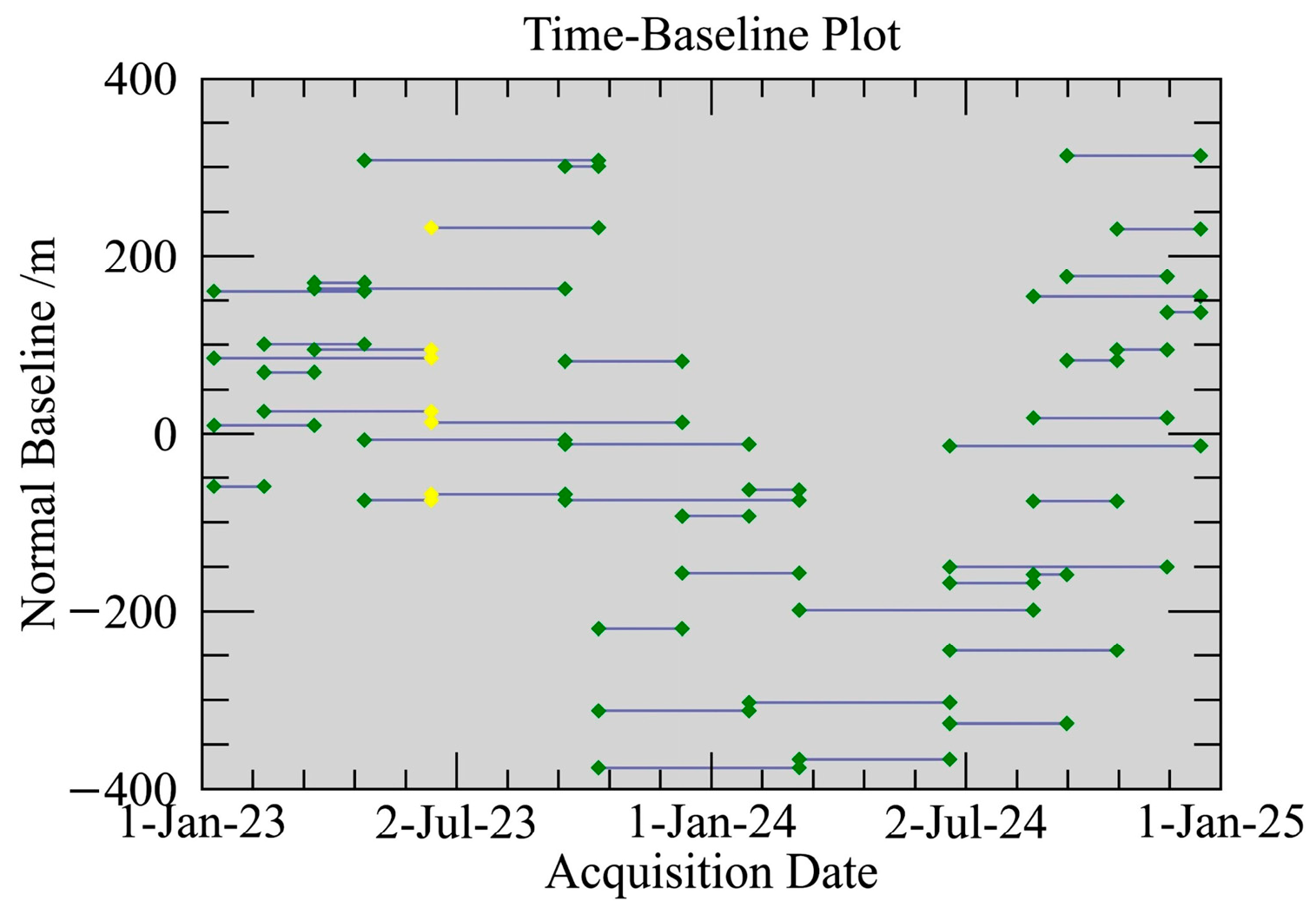
(2) The sixteen preprocessed Sentinel-1A images were paired using the connection graph tool. Under the optimal combination, the maximum number of pairs was 120, as shown in Figure 3 and Figure 4.
(3) For all interferometric pairs, coherence generation, flattening, filtering, and phase unwrapping were performed. These steps ensured that all data pairs were registered to a super master image, generating a series of unwrapped phase maps [24]. The results showed that although flipping occurred in the coherence coefficient maps and unwrapped phase maps, there was no significant loss of coherence. Therefore, no pairs were discarded in this study.
(4) The key steps of orbit refinement and re-flattening involve estimating and removing constant phase and residual phase ramps after unwrapping. Ground Control Points (GCPs) were used for re-flattening across all data pairs. GCPs needed to be effectively utilized in the unwrapped results of all pairs, requiring selection on a pair with good coherence [25]. However, due to varying coherence levels across pairs, it was challenging to find an ideal set of GCPs applicable to all pairs. Thus, 27 GCPs were selected, which met the criteria as closely as possible and were usable across all pairs.
(5) Step 1 of SBAS inversion was to estimate deformation rates and residual topography.
(6) Step 2 of SBAS inversion was to calculate time-series displacements. Using the deformation rates obtained in Step 1, customized atmospheric filtering was applied to estimate and remove atmospheric phases, yielding cleaner final time-series displacement results [26].
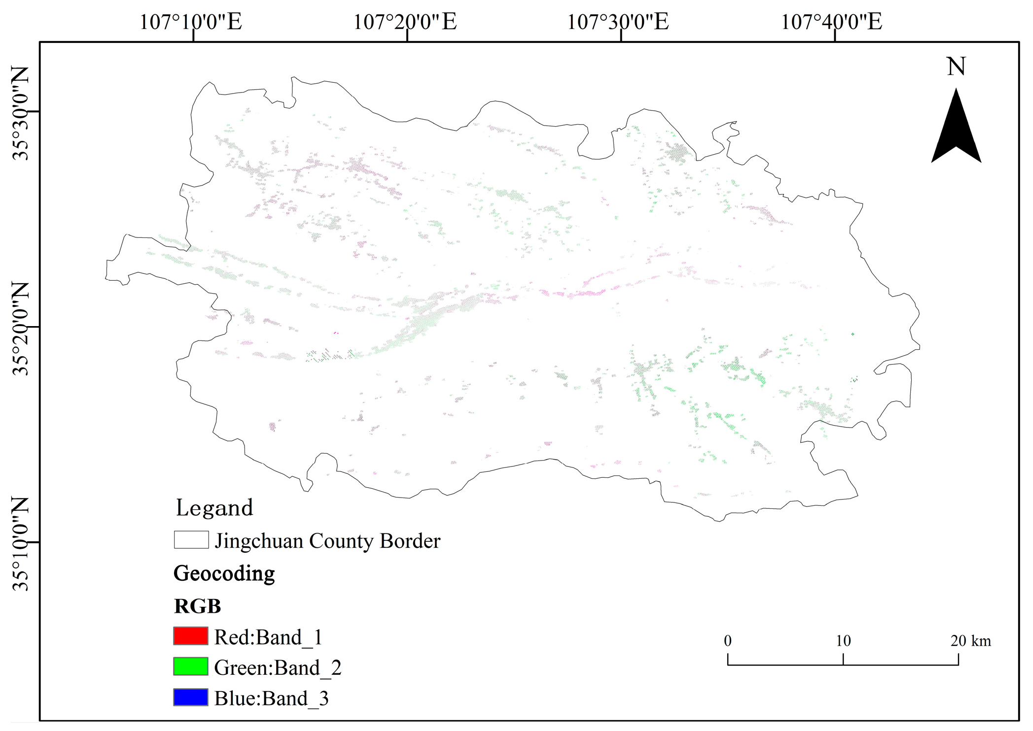
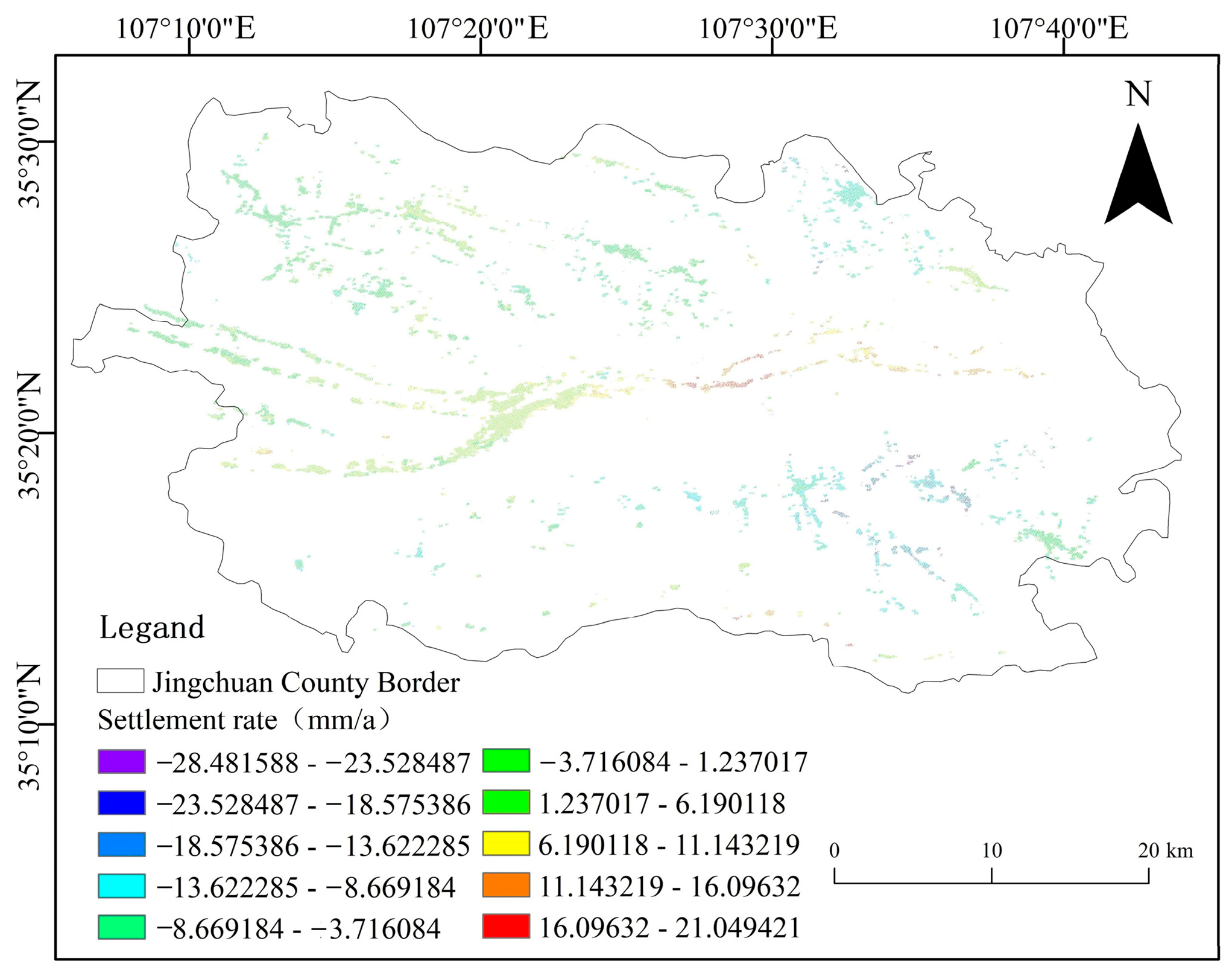
(7) The results from Step 2 were geocoded to project the ground deformation results in the correct direction, as shown in Figure 5, the ground deformation status of the study area was visualized, as shown in Figure 6.
It should be specifically noted that Figure 5 employed a false color composite technique. The colors shown are not the true colors of the features but are instead generated by combining different bands (Red: Band_1, Green: Band_2, Blue: Band_3) to enhance the visualization of feature characteristics. When these three bands are synthesized in RGB mode, the differences in reflectance of various features across the bands are converted into combinations of red, green, and blue, resulting in mixed colors such as purple and green.
Positive values indicate ground uplift; negative values indicate ground subsidence (mm/year). Green indicates low or no significant deformation. Red indicates ground uplift caused by activities such as construction. Blue indicates ground subsidence caused by groundwater changes, mining, gravity or other geological processes, typically marking potential landslide areas.

3.2. Object-Oriented Classification Method

The object-oriented classification method abstracts landslide features into objects, thereby identifying and classifying landslides. Compared to traditional pixel-level classification methods, the object-oriented classification method reflects the overall characteristics and spatial relationships of ground objects [27,28].
(1) Preprocessing such as geometric correction and radiometric correction were applied to the Landsat 8 imagery using ENVI 5.6. The images were then clipped according to the study area boundary [29].
(2) Radiometric calibration converted the digital values in the image into real-world physical quantities, such as ground reflectance, radiance, and temperature. Through a series of transformations, these values could reflect the actual radiance or reflectance of surface features.
(3) FLAASH is an advanced atmospheric correction method used to remove the effects of atmospheric conditions on surface reflectance in remote sensing images [30]. After applying FLAASH, the image data more accurately reflected surface reflectance characteristics, improving the accuracy of subsequent ground object classification and deformation detection.
(4) The Nearest Neighbor Diffusion method was used to fuse high-resolution panchromatic images with low-resolution multispectral images. Since the resolution of Landsat 8 images after radiometric calibration and FLAASH was relatively low, fusing them with high-resolution images enhanced the visual quality and analytical capability [31].
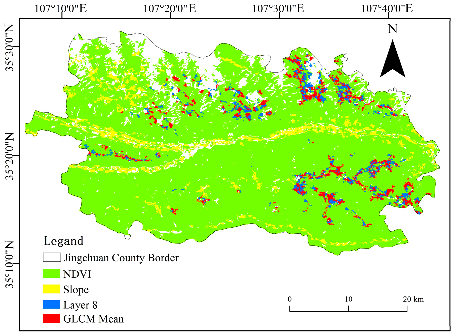
(5) Multiscale segmentation merged adjacent pixels or smaller segmented objects while maintaining homogeneity and heterogeneity. The optimal control factors were as follows: the segmentation scale was 83, shape factor was 0.5, spectral factor was 0.5, smoothness was 0.4, and compactness was 0.6 [32]. After repeated adjustments, the rule set for extracting potential landslides included the Normalized Difference Vegetation Index (NDVI), gradient, Landsat 8 infrared band (Layer 8), and Gray-Level Co-occurrence Matrix mean (GLCM mean). The calculation method for NDVI is shown in Equation (1), and the threshold range for each feature is listed in Table 2.
NDVI = N I R R N I R + R
where NIR is the reflectivity of the near-infrared band, R is the reflectivity of the red band.
The blue regions were identified as potential landslides based on Table 2, as shown in Figure 7.

3.3. Identification Results of Potential Landslides

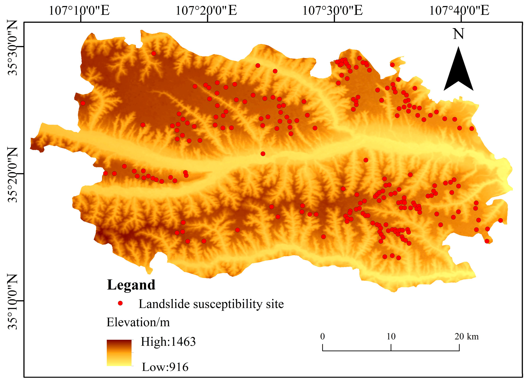
Surface deformation and potential landslides in the study area were identified by integrating SBAS-InSAR and the object-oriented classification method. Combined with field investigations conducted from 11 March to 17 March 2025, a total of 246 potential landslides were confirmed, as shown in Figure 8.
The area of the 246 potential landslides is 0.427 km2, while the volume is 2.161 × 10⁶ m3. The largest potential landslide is the Zhangmaocai Landslide, with an area of 0.013 km2 and a volume of 8.332 × 10⁴ m3. The DEM of the study area was resampled into 10 m × 10 m grids using ArcGIS 10.2, and the number of potential landslide grids was 6160. Since subsequent landslide susceptibility modeling requires both positive and negative samples, an additional 6160 grids were randomly selected from non-landslide areas to serve as negative samples. The method for selecting non-landslide grids was as follows: set the elevation to no more than 1200 m and the gradient to no more than 5°, then manually select non-landslide grids that are relatively distant from the landslide grids from the eligible grids.

4. LSM in the Study Area

4.1. Selection of Hazard Factors

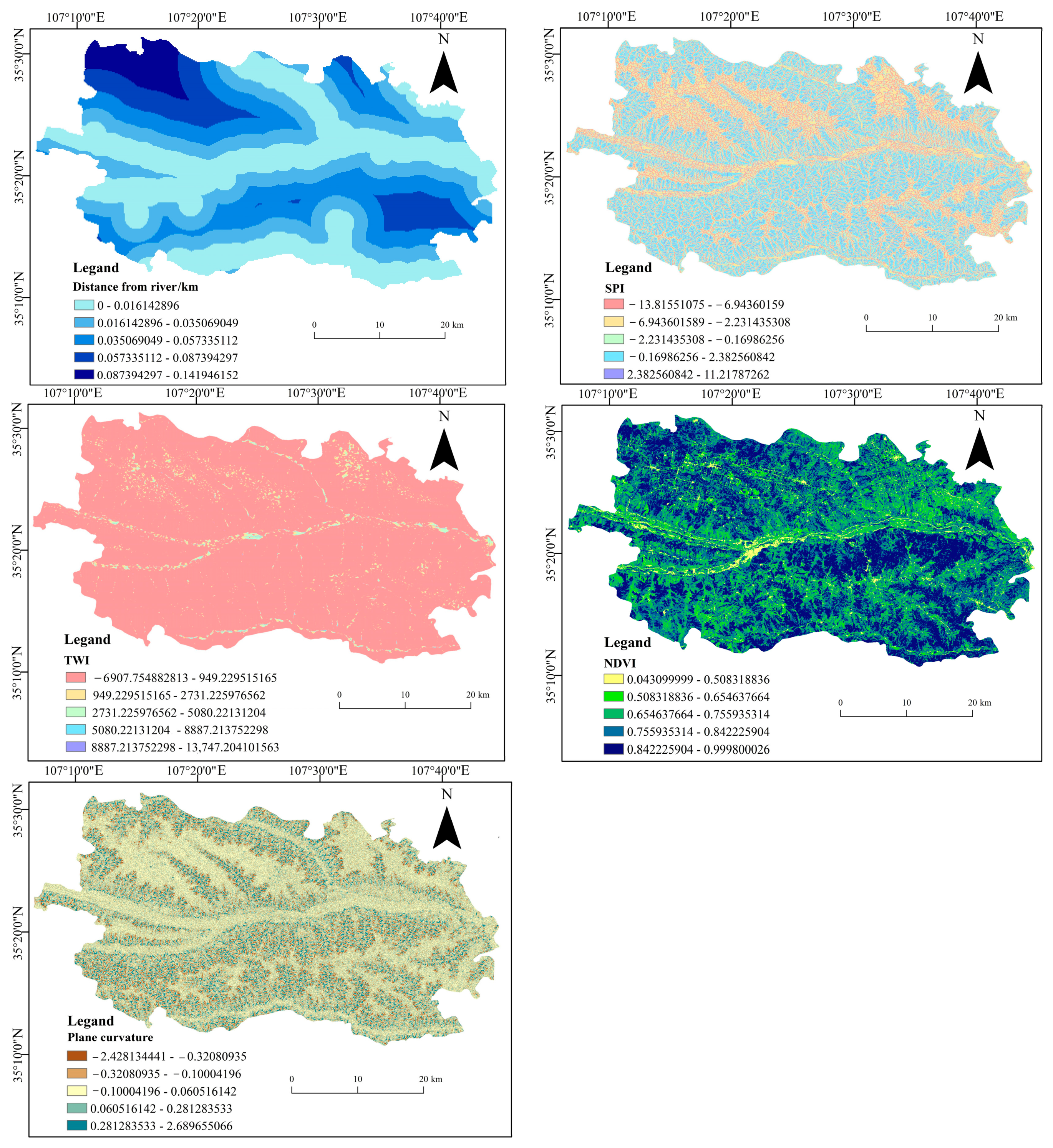
The landslide disaster-prone environment involves topographic and geological factors (elevation, gradient, slope aspect, plane curvature (PLC), profile curvature (PRC), lithology, distance from fault), hydrological and vegetation factors (distance from river, topographic wetness index (TWI), sediment transport index (STI), stream power index (SPI), NDVI), and human activity factors (distance from road, land use) [33,34]. Among them, TWI quantifies the influence of terrain on hydrological processes, describing the degree of surface saturation runoff, which increases with contributing area accumulation. STI represents the comprehensive terrain variable for slope sediment transport, indicating the degree to which surface sands and other materials are transported by water flow. SPI is an important parameter that characterizes the surface water erosion capacity and is used to identify strong flow paths formed by water accumulation and locations prone to gully erosion [35,36]. The calculation methods for SPI, STI, and TWI are shown in Equations (2) to (4) [37].
SPI = A s tan β
STI = A s 22.13 0.6 sin β 0.0896 1.3
TWI = ln A s tan β
where As is the area of the upstream area through which the surface water flows per unit contour length, which can be calculated from the cumulative area of the confluence and the length of the upstream water flow; β is the terrain slope gradient.
The bivariate correlation analysis method was used to calculate the Pearson correlation coefficient between any two hazard factors, as shown in Table 3.
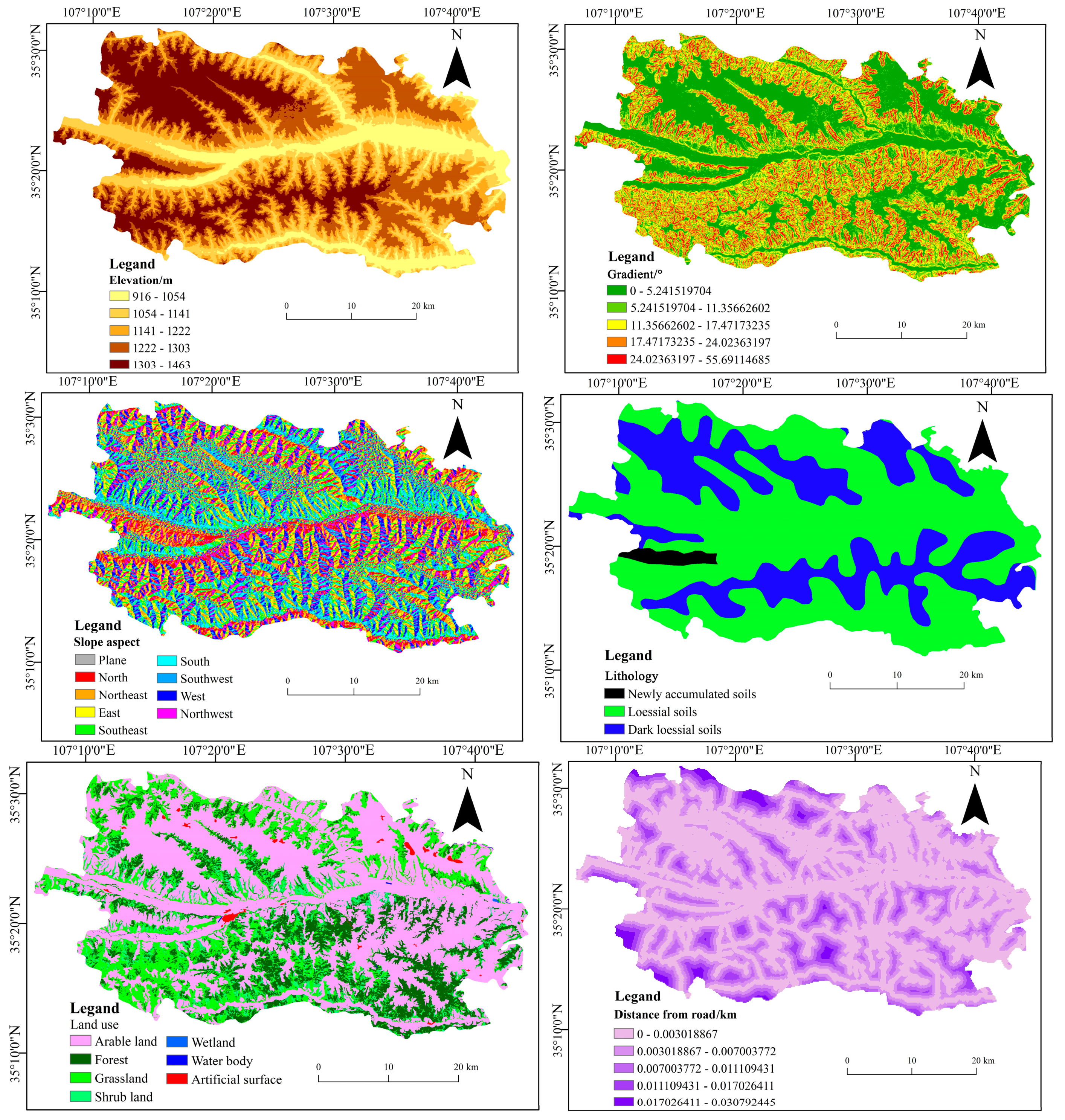
Since STI, distance from fault and PRC had Pearson correlation coefficients with absolute values ≥ 0.4 more than once, they were excluded. The remaining eleven hazard factors are elevation, gradient, slope aspect, lithology, land use, distance from road, distance from river, SPI, TWI, NDVI, and PLC. The eight quantitative factors were classified according to Yin et al. [38] and Li et al. [39], while the three qualitative factors were classified based on their natural attributes, as shown in Table 4.
The DEM of the study area was resampled into 10 m × 10 m grids using ArcGIS 10.2. The classification maps for the eleven hazard factors were generated based on Table 4, as shown in Figure 9.

4.2. Model Overview

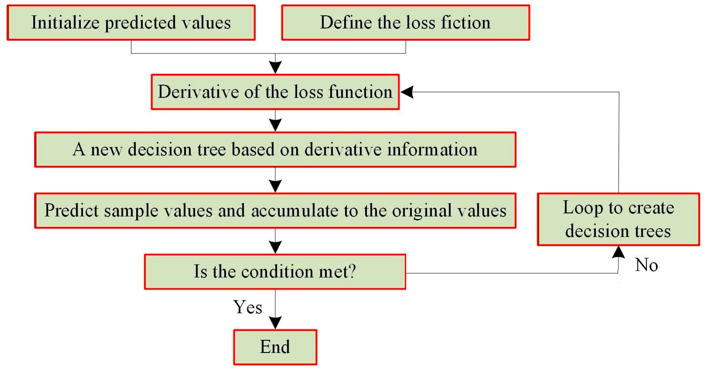
Compared to the traditional Gradient Boosting Decision Tree (GBDT) algorithm, the XGBoost model utilizes a second-order Taylor expansion to simplify the calculation when solving the loss function and introduces regularization terms such as L1 and L2 into the objective function, resulting in higher computational efficiency and improved overfitting prevention capabilities [40]. CNN leverages the structural advantages of parameter sharing and local connectivity, enabling efficient processing of grid-like data without relying on additional features. Compared to traditional fully connected networks, CNN exhibits fewer parameters and stronger representational power when handling high-dimensional data. The Blending-XGBoost-CNN model integrates the XGBoost model and CNN model through the Blending framework, which can enhance the overall performance [41]. The XGBoost model, CNN model, and Blending-XGBoost-CNN model were constructed based on Python 3.12 for LSM.

4.2.1. The XGBoost Model

The XGBoost model implements machine learning under the Gradient Boosting framework, capable of adapting to complex nonlinear relationships. It possesses strong parallel processing capabilities and high interpretability, effectively addressing overfitting issues. Additionally, it offers advantages such as fast computation speed and the ability to handle large-scale data. The XGBoost model is an improvement over the Gradient Boosting algorithm, optimizing the decision tree structure within the Gradient Boosting framework. It achieves a more precise approximation of the loss function and integrates first and second derivatives using CPU multi-threaded parallel computing [42]. The calculation method for the predicted values of the XGBoost model is shown in Equation (5), and the loss function is shown in Equation (6).
y ^ t = k = 1 t f k x i = y ^ t 1 + f t x i
L ϕ = i = 1 n l y ^ t , y ( t ) + k Ω f
where y ^ t is the final predicted landslide susceptible probability, y ^ t 1 is the accumulated landslide susceptible probability from previous iterations, xi is the feature values related to landslides, fk(xi) is the contribution of the newly generated tree in the current iteration to the landslide susceptible probability, t is the number of model iterations, n is the number of training samples, l( ) is the loss function for a single sample, y(t) is the true label value of the training sample, and Ω(f) is the regularization term, which defines the complexity of the model [43], as shown in Equation (7).
Ω f = γ T + λ ω 2 2
where γ and λ are manually set parameters, w is a vector formed by the values of all leaf nodes in the decision tree, and T is the number of leaf nodes. The computational process of the XGBoost model is shown in Figure 10.

4.2.2. CNN Model

The one-dimensional CNN network used in this study consisted of one input layer, one convolutional layer, one pooling layer, four fully connected layers, and one output layer. The network structure is shown in Figure 11.
The input layer was used to recognize one-dimensional vectors composed of hazard factor values. The convolutional layer included nine convolutional kernels, which were used to perform matrix dot product operations on the one-dimensional vectors to extract basic features of the data. The calculation method is shown in Equation (8) [44].
C j = i = 1 11 f ω j x i + b j
where Cj is the output of the j-th convolutional kernel, i is the position of the convolutional layer operation, xi (i = 1, 2, …, 11) is the hazard factor data corresponding to the convolutional window, f is the nonlinear activation function, and wj and bj are the weight and bias, respectively.
The pooling layer was used to filter the feature data extracted by the convolutional layer, reducing the number of feature vectors while retaining effective information and preventing overfitting [45]. Taking the max pooling operation for two-dimensional data as an example, the calculation method is shown in Equation (9).
O i = max i N a i n × n
where Oi is the output value of the max pooling operation, i is the pooling position, and a i n × n is the hazard factor data corresponding to the max pooling operation at position i.
The fully connected layer was used to integrate local information with categorical features, serving as a “classifier”, and transmitted the information to the next layer through an activation function. The SoftMax function was employed for multi-class classification [46]. The SoftMax function mapped output values to the range [0, 1] and ensured that the sum of the output values from all nodes was 1. In the binary classification algorithm, the output layer consisted of two neurons representing landslide and non-landslide, which were derived from the SoftMax activation function. The calculation method is shown in Equation (10).
S r = e z r r = 1 R e z r
where Sr is the value of the SoftMax function, e is the natural constant, and e z r is the exponential value of the r-th element in the array Z.
The backpropagation algorithm helps optimize CNN parameters, enabling the model’s loss value to reach a convergent state. This study employed the cross-entropy loss function to measure the distance between two probability distributions. The smaller the cross-entropy loss value, the closer the probability distributions of the true samples and the predicted samples are [47]. The cross-entropy loss function is shown in Equation (11).
L o s s = 1 T v = 1 T y v log y ^ v + 1 y v log 1 y ^ v
where Loss is the value of the cross-entropy loss function; yv and y ^ v are the true label and predicted label of the v-th input sample, respectively.

4.2.3. The Blending-XGBoost-CNN Model

Blending is a variant of the Stacking model, introduced in the Netflix competition, which uses a two-layer structure consisting of base models and a meta-model. The base models learn the relationship between data and labels, generate predicted values, and output them to form a new feature dataset. The meta-model then learns from and makes predictions on this new feature dataset [48]. Unlike traditional Stacking, Blending reserves a portion of the data as an independent test set, which does not participate in the training of the base models. The base models are trained only on the remaining data and generate predictions based on the independent test set to improve computational efficiency and avoid data leakage [49]. In this study, the Blending framework was used to connect the XGBoost model and CNN model to construct the Blending-XGBoost-CNN model for LSM.

4.3. LSM Results

70% of landslide grids (4312) and 70% of non-landslide grids (4312) were selected as training samples, while the remaining 30% of landslide grids (1848) and 30% of non-landslide grids (1848) were validation samples. The input values for each sample were the hazard factors, while output value was 1 for landslide grids and 0 for non-landslide grids [50]. The XGBoost model, CNN model, and Blending-XGBoost-CNN model were trained using the training samples. The trained models were used to calculate the output values for all 14,642,667 grids in the study area, which represented the landslide susceptible probability. The results show that the output values for the XGBoost model range from 0.093 to 0.982, for the CNN model from 0.041 to 0.886, and for the Blending-XGBoost-CNN model from 0.087 to 0.945.
TPR was used to measure the proportion of landslide grids that the model correctly predicted [51], as shown in Equation (12).
T P R = T P T P + F N
where TP is the number of landslide grids that the model correctly predicted, and FN is the number of landslide grids that the model incorrectly predicted.
FPR was used to measure the proportion of landslide grids that the model incorrectly predicted, as shown in Equation (13).
F P R = F P F P + T N
where FP is the number of non-landslide grids that the model incorrectly predicted, and TN is the number of non-landslide grids that the model correctly predicted.
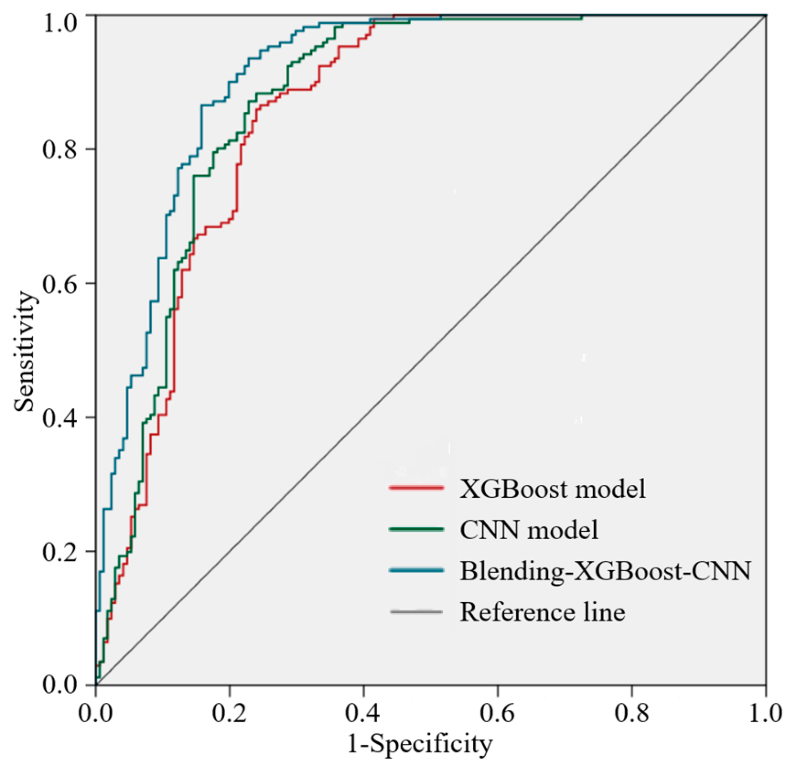
ROC curves were plotted with TPR and FPR as the vertical and horizontal axes, respectively. The area under the curve (AUC) is a commonly used metric to evaluate the model’s performance. The AUC value ranges from 0 to 1, and when the AUC is close to 1, the model performs well and can effectively distinguish between positive and negative samples [52]. The ROC curves for the XGBoost model, CNN model, and Blending-XGBoost-CNN model are shown in Figure 12, and the AUC-related statistical values are shown in Table 5.
Precision was also used for evaluating the model’s performance. It measures the proportion of landslide grids correctly predicted [53]. The calculation method is shown in Equation (14).
Precision = T P T P + F P
The Precisions for the XGBoost model, CNN model, and Blending-XGBoost-CNN model are 0.77, 0.79, and 0.83, respectively. The Blending-XGBoost-CNN model has the highest AUC and Precision, indicating that this model outperforms the XGBoost model and CNN model. Therefore, it can be promoted and applied in landslide monitoring and early warning systems.
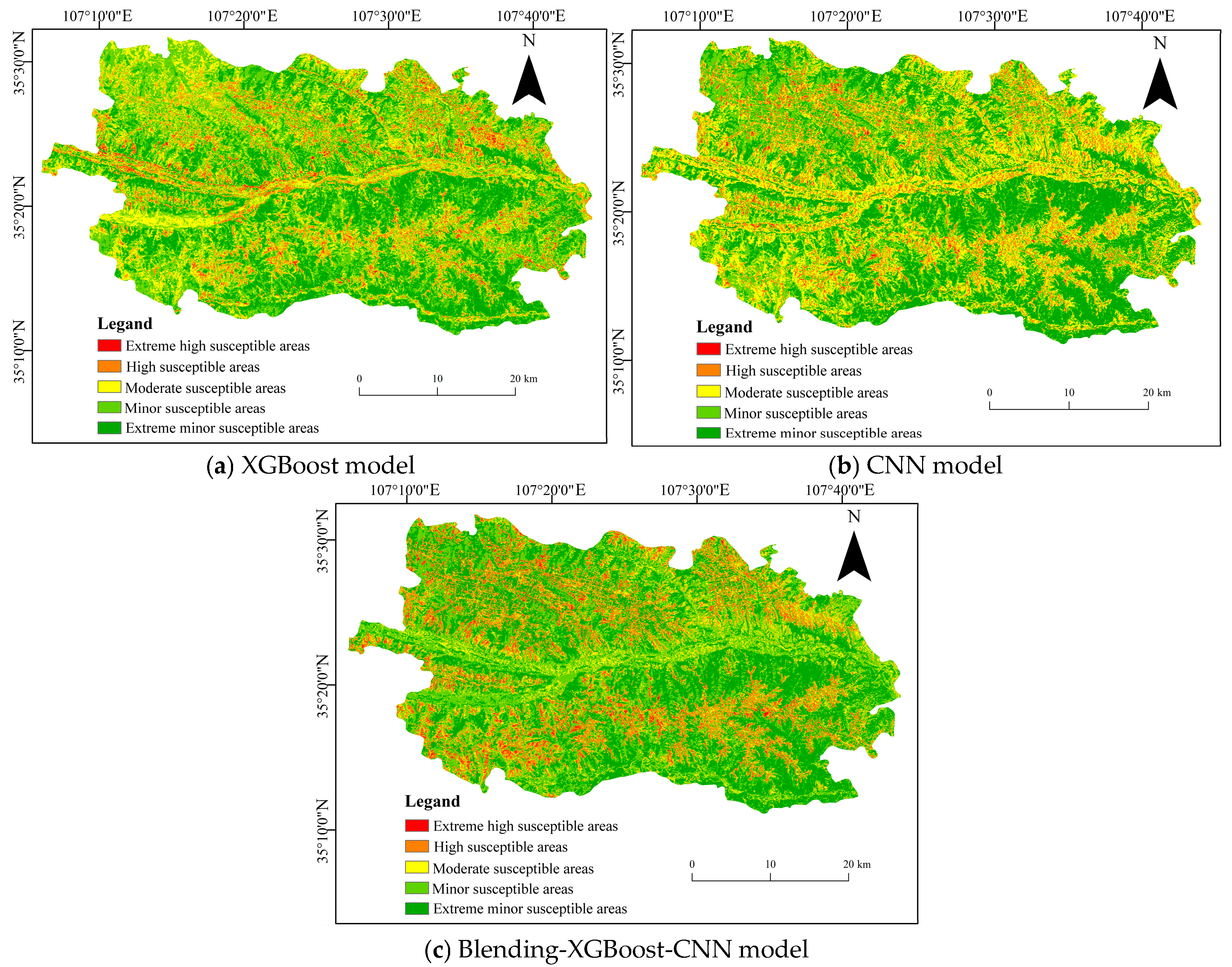
The landslide susceptible probabilities were divided into five levels: extreme minor susceptible [0.000, 0.200), minor susceptible [0.200, 0.400), moderate susceptible [0.400, 0.600), high susceptible [0.600, 0.800), and extreme high susceptible [0.800, 1.000] [54]. Landslide susceptible zoning maps for the XGBoost model, CNN model, and Blending-XGBoost-CNN model were generated based on ArcGIS 10.2, as shown in Figure 13.
Based on the LSM results of the Blending-XGBoost-CNN model, the extreme high susceptible areas, high susceptible areas, moderate susceptible areas, minor susceptible areas, and extreme minor susceptible areas account for 6.24% (91.4 km2), 15.07% (220.6 km2), 29.15% (426.8 km2), 30.58% (447.7 km2), and 18.96% (277.8 km2) of the total area, respectively. Among the 6160 landslide grids, 69.15% (4260 grids), 16.35% (1007 grids), 8.26% (509 grids), 4.06% (250 grids), and 2.18% (134 grids) are in these areas, respectively.

5. Discussions

LSM results of the Blending-XGBoost-CNN model were discussed based on the Geodetector considering the eleven hazard factors as independent variables [55].

5.1. Factor Detector

A larger q indicates a stronger explanatory power, meaning the spatial heterogeneity is more pronounced as a single hazard factor in the Factor Detector function of Geodetector [56]. The explanatory power of hazard factors except for SPI on landslide susceptibility passed the significance tests, indicating that q was statistically significant, as shown in Table 6. The explanatory power was classified into four levels: very high (0.6 ≤ q ≤ 1.0), high (0.3 ≤ q < 0.6), moderate (0.15 ≤ q < 0.3), and low (0.0 ≤ q < 0.15).
NDVI and gradient are key factors determining landslide occurrence. Elevation, slope aspect, distance from river, and land use also play significant roles in landslide occurrence. the contributions of TWI and lithology to landslide occurrence are relatively small, while PLC and distance from road have q values close to 0, indicating their influences on the landslide occurrence are minimal.
Li et al. [39] conducted a similar study in Yiyuan County, Zibo City, Shandong Province. The results showed that elevation and land use were the key determinants of landslide susceptibility, while SPI and PLC had almost no effect. These conclusions differed significantly from those obtained in this paper. The main reasons include: (1) the study area is located on the Loess Plateau, where vegetation coverage is generally low. Vegetation can intercept rainfall and reduce flow velocity. Therefore, slopes with higher NDVI are less likely to experience landslides, while the opposite is true for slopes with lower NDVI. (2) Loess has high porosity and well-developed vertical joints, allowing it to remain stable in a near-vertical state under natural conditions. However, when saturated with water, the structure of loess rapidly disintegrates, leading to significant changes in gradient.

5.2. Interaction Detector

Through the Interaction Detector function of Geodetector, the q of any two combined hazard factors increased to varying degrees compared to that of any single factor [57]. The explanatory power on landslide susceptibility exhibits two types of interactions: Nonlinear-Enhance (NE) and Bi-Enhance (BE). NE and BE both indicate that the two factors have nonlinear effects on landslide susceptibility. However, NE follows only a single nonlinear rule, resulting in a relatively simple influencing mechanism. In contrast, BE involves multiple NE operations, adheres to no fewer than two nonlinear rules, and exhibits a more complex influencing mechanism, as shown in Table 7.
The interactions between eleven pairs of hazard factors are BE, including (slope aspect, NDVI), (PLC, NDVI), (PLC, slope aspect), (distance from river, slope aspect), (distance from river, PLC), (distance from road, PLC), (lithology, TWI), (lithology, PLC), (lithology, distance from river), (lithology, distance from road), (land use, lithology). Among them, the interactions between lithology and the other five factors, as well as between PLC and the other five factors, are BE. Similarly, the interactions between slope aspect and the other three factors, and between distance from river and the other three factors, are also BE. This indicates that these four hazard factors have more complex triggering mechanisms for landslides. The interaction of hazard factors not only increases landslide risk but also leads to more complex disaster patterns. Therefore, when formulating landslide mitigation strategies, it is essential to fully consider the complex relationships among hazard factors. This approach enables more effective landslide prediction and prevention.

6. Conclusions

(1) To provide the data required for LSM, potential landslides in Jingchuan County were identified using two remote sensing interpretation methods: surface subsidence was interpreted using SBAS-InSAR with Sentinel-1A ascending orbit images; landslides were interpreted using the object-oriented classification method with Landsat 8 images. A total of 246 potential landslides were identified, covering an area of 0.427 km2, and a volume of 2.161 × 10⁶ m3. The largest potential landslide was at Zhangmaocai Village, covering an area of 0.013 km2 with a volume of 8.332 × 10⁴ m3.
(2) Based on the Pearson bivariate correlation analysis, eleven landslide hazard factors were determined. Landslide susceptible zoning maps for Jingchuan County were generated using the XGBoost model, CNN model, and Blending-XGBoost-CNN model. Among these, the Blending-XGBoost-CNN model performed the best, with landslide susceptible probabilities ranging from 0.087 to 0.945. The extreme high susceptible areas, high susceptible areas, moderate susceptible areas, minor susceptible areas, and extreme minor susceptible areas accounted for 6.24% (91.4 km2), 15.07% (220.6 km2), 29.15% (426.8 km2), 30.58% (447.7 km2), and 18.96% (277.8 km2) of the total area. Among the 6160 landslide grids, 69.15% (4260 grids), 16.35% (1007 grids), 8.26% (509 grids), 4.06% (250 grids), and 2.18% (134 grids) are in these areas, respectively.
(3) NDVI and gradient are key factors determining landslide occurrence. Elevation, slope aspect, distance from river, and land use also play significant roles in landslide occurrence. The contribution of TWI and lithology to landslide occurrence is relatively small, while PLC and distance from road have q values close to 0, indicating their influence on the landslide occurrence is minimal. When any two hazard factors are combined, their q values increase to varying degrees compared to those of individual factors. The interaction of multiple hazard factors not only increases landslide risk but also leads to more complex disaster patterns.
(4) This study utilized remote sensing interpretation to identify potential landslides and conducted LSM based on the XGBoost model, CNN model, and Blending-XGBoost-CNN model, respectively. The results can provide a theoretical basis for landslide prevention-oriented land use planning. However, further improvements can be made in the following aspects: (1) With the advancement of artificial intelligence technology, advanced brain-like neural network models can offer more approaches for LSM, and there is still significant room for improving the accuracy of the results. (2) This study analyzed the interaction of hazard factors on landslide susceptibility and categorized them into NE and BE. However, this research was still in its early stages, and the specific mechanisms of influence remain unclear. (3) Although the method proposed in this paper demonstrated high applicability to the study area, the limited size of the area and its unique geological characteristics mean that the applicability of the method to other regions with distinct geological features remains unclear. The authors intend to conduct further in-depth research on these topics in the future.

Author Contributions

Methodology, B.M., F.G., X.S. and M.L.; Software, C.Y.; Formal analysis, C.Y., X.S. and M.L.; Investigation, B.M. and F.G.; Data curation, C.Y.; Writing—original draft, B.M. and X.S.; Writing—review & editing, C.Y. and M.L.; Project administration, F.G.; Funding acquisition, C.Y. All authors have read and agreed to the published version of the manuscript.

Funding

This research was funded by National Natural Science Foundation of China, grant number [51808327] and Natural Science Foundation of Shandong Province, grant number [ZR2019PEE016].

Institutional Review Board Statement

Not applicable.

Informed Consent Statement

Not applicable.

Data Availability Statement

The original contributions presented in this study are included in the article. Further inquiries can be directed to the corresponding author.

Conflicts of Interest

The authors declare no conflict of interest.

References

  1. Longoni, L.; Scaioli, A.; Panzeri, L.; Arosio, D.; Corti, M.; Hojat, A.; Papini, M. A new Landslide Investigation and Simulation Archive through downscaled landslide experiments. Sci. Data 2025, 12, 1668. [Google Scholar] [CrossRef]
  2. Yin, C.; Tian, W.B.; Che, F.; Guo, B.; Wang, S.P.; Jia, Z.R. Model tests and numerical simulations on hydraulic fracturing and failure mechanism of rock landslides. Nat. Hazards 2023, 115, 1977–1996. [Google Scholar] [CrossRef]
  3. Trinh, T.; Luu, B.T.; Nguyen, D.H.; Le, T.H.T.; Pham, S.V.; Thi, N.V. A study of non-landslide samples and weights for mapping landslide susceptibility using regression and clustering methods. Earth Sci. Inform. 2023, 16, 4009–4034. [Google Scholar] [CrossRef]
  4. Oliveira, S.C.; Zêzere, J.L.; Garcia, R.A.C.; Pereira, S.; Vaz, T.; Melo, R. Landslide susceptibility assessment using different rainfall event-based landslide inventories: Advantages and limitations. Nat. Hazards 2024, 120, 9361–9399. [Google Scholar] [CrossRef]
  5. Li, Y.M.; Ji, P.K.; Liu, S.Y.; Zhao, J.Z.; Yang, Y.M. Susceptibility evaluation of highway landslide disasters based on SBAS-InSAR: A case study of S211 highway in Lanping County. Nat. Hazards 2025, 121, 2587–2612. [Google Scholar] [CrossRef]
  6. Jin, B.J.; Zeng, T.R.; Yin, K.L.; Gui, L.; Guo, Z.Z.; Wang, T.F. Dynamic landslide susceptibility mapping based on the PS-InSAR deformation intensity. Environ. Sci. Pollut. Res. 2024, 31, 7872–7888. [Google Scholar] [CrossRef]
  7. Li, Y.C.; Chen, J.P.; Tan, C.; Li, Z.H.; Zhang, Y.S.; Yan, J.H. Deformation and potential failure analysis of a giant old deposit in the southeastern margin of the Qinghai-Tibet Plateau based on SBAS-InSAR and numerical simulation. Bull. Eng. Geol. Environ. 2023, 82, 58. [Google Scholar] [CrossRef]
  8. Zheng, X.S.; Lu, W.J.; Jiang, R.C.; Li, J.H.; Zhang, L.M. Analysis of landslide on Meizhou-Dapu expressway based on satellite remote sensing. Geoenviron. Disasters 2025, 12, 25. [Google Scholar] [CrossRef]
  9. Arpitha, G.A.; Choodarathnakara, A.L.; Rajaneesh, A.; Sinchana, G.S.; Sajinkumar, K.S. Creation of a Landslide Inventory for the 2018 Storm Event of Kodagu in the Western Ghats for Landslide Susceptibility Mapping Using Machine Learning. J. Indian Soc. Remote Sens. 2024, 52, 2443–2459. [Google Scholar] [CrossRef]
  10. Qin, H.; Wang, J.Z.; Mao, X.; Zhao, Z.A.; Gao, X.Y.; Lu, W.J. An Improved Faster R-CNN Method for Landslide Detection in Remote Sensing Images. J. Geovis. Spat. Anal. 2023, 8, 2. [Google Scholar] [CrossRef]
  11. Yan, Y.Q.; Guo, C.B.; Zhang, Y.N.; Song, D.G.; Qiu, Z.D. Comprehensive evaluation and prediction of potential long-runout landslide in Songrong, Tibetan Plateau: Insights from remote sensing interpretation, SBAS-InSAR, and Massflow numerical simulation. Bull. Eng. Geol. Environ. 2024, 83, 198. [Google Scholar] [CrossRef]
  12. Chandra, N.; Vaidya, H. Automated detection of landslide events from multi-source remote sensing imagery: Performance evaluation and analysis of YOLO algorithms. J. Earth Syst. Sci. 2024, 133, 127. [Google Scholar] [CrossRef]
  13. Choi, S.K.; Ranirez, R.A.; Lim, H.H.; Kwon, T.H. Multi-source remote sensing-based landslide investigation: The case of the August 7, 2020, Gokseong landslide in South Korea. Sci. Rep. 2024, 14, 12048. [Google Scholar] [CrossRef]
  14. Handwerger, A.L.; Lacroix, P.; Bell, A.F.; Booth, A.M.; Huang, M.H.; Mudd, S.M.; Bürgmann, R.; Fielding, E.J. Multi-sensor remote sensing captures geometry and slow-to-fast sliding transition of the 2017 Mud Creek landslide. Sci. Rep. 2025, 15, 29831. [Google Scholar] [CrossRef]
  15. Yang, X.W.; Chen, D.N.; Dong, Y.H.; Xue, Y.M.; Qin, K.X. Identification of potential landslide in Jianzha county based on InSAR and deep learning. Sci. Rep. 2024, 14, 21346. [Google Scholar] [CrossRef]
  16. Yin, C.; Li, H.R.; Che, F.; Li, Y.; Liu, D. Susceptibility mapping and zoning of highway landslide disasters in China. PLoS ONE 2020, 15, e0235780. [Google Scholar] [CrossRef]
  17. Mao, X.C.; Liu, P.; Deng, H.; Liu, Z.K.; Li, L.J.; Wang, Y.S.; Ai, Q.X.; Liu, J.X. A Novel Approach to Three-Dimensional Inference and Modeling of Magma Conduits with Exploration Data: A Case Study from the Jinchuan Ni-Cu Sulfide Deposit, NW China. Nat. Resour. Res. 2023, 32, 901–928. [Google Scholar] [CrossRef]
  18. Sun, D.; Zhang, C.Y.; Zhang, S.A.; Xu, J.D.; Tao, Z.G.; Wu, M.L.; Li, D.X.; Zhang, G.H.; Liu, Y.P.; Wang, F.N.; et al. Hydraulic Fracturing In-Situ Stress Measurements and Large Deformation Evaluation of 1000m-Deep Soft Rock Roadway in Jinchuan No. 2 Mine, Northwestern China. Rock Mech. Rock Eng. 2025, 58, 2781–2801. [Google Scholar] [CrossRef]
  19. Chen, W.; Wang, J.L.; Xie, X.S.; Hong, H.Y.; Trung, N.V.; Bui, D.T.; Wang, G.; Li, X.R. Spatial prediction of landslide susceptibility using integrated frequency ratio with entropy and support vector machines by different kernel functions. Environ. Earth Sci. 2016, 75, 1344. [Google Scholar] [CrossRef]
  20. Jin, T.; Zhang, X.; Xie, J.C.; Liang, J.C.; Wang, T.T. Study on hydrological response of runoff to land use change in the Jing River Basin, China. Environ. Sci. Pollut. Res. 2023, 30, 101075–101090. [Google Scholar] [CrossRef]
  21. Chen, X.W.; Chen, J.P.; Wang, G.H.; Zhang, Q.; Zheng, Y.W. Mining Subsidence Based on Integrated SBAS-InSAR and Unmanned Aerial Vehicles Technology. J. Ocean Univ. China 2025, 24, 113–129. [Google Scholar] [CrossRef]
  22. Ijaz, Z.; Zhao, C.; Ijaz, N.; Rehman, Z.; Ijaz, A. Novel application of Google earth engine interpolation algorithm for the development of geotechnical soil maps: A case study of mega-district. Geocarto Int. 2022, 37, 18196–18216. [Google Scholar] [CrossRef]
  23. Duan, M.; Li, Z.W.; Xu, B.; Jiang, W.P.; Cao, Y.M.; Xiong, Y.; Wei, J.C. Turbulent atmospheric phase correction for SBAS-InSAR. J. Geod. 2024, 98, 81. [Google Scholar] [CrossRef]
  24. Zhang, J.Y.; Gao, J.; Gao, F.Z. Time series land subsidence monitoring and prediction based on SBAS-InSAR and GeoTemporal transformer model. Earth Sci. Inform. 2024, 17, 5899–5911. [Google Scholar] [CrossRef]
  25. Tao, Q.X.; Liu, R.X.; Li, X.P.; Gao, T.F.; Chen, Y.; Xiao, Y.X.; He, H.Z.; Wei, Y.G. A method for monitoring three-dimensional surface deformation in mining areas combining SBAS-InSAR, GNSS and probability integral method. Sci. Rep. 2025, 15, 2853. [Google Scholar] [CrossRef]
  26. Niu, W.; Hu, X.N.; Lin, B.; Meng, F.Q.; Zhang, Y.; Zhao, J. Detection and Monitoring of Potential Geological Disaster Using SBAS-InSAR Technology. KSCE J. Civ. Eng. 2023, 27, 4884–4896. [Google Scholar] [CrossRef]
  27. Dahiya, N.; Singh, S.; Gupta, S. Comparative Analysis and Implication of Hyperion Hyperspectral and Landsat-8 Multispectral Dataset in Land Classification. J. Indian Soc. Remote Sens. 2023, 51, 2201–2213. [Google Scholar] [CrossRef]
  28. Brahim, S.V.; Olatunji, A.S.; Umaru, A.O.; Olisa, O.G.; Reyoug, S.S.; Hamoud, A. Lithological, structural, and alteration mapping of uraniferous granitoid using Landsat 8, in the oriental part of the Reguibat shield, northern Mauritania. Arab. J. Geosci. 2024, 17, 170. [Google Scholar] [CrossRef]
  29. Singh, G.; Dahiya, N.; Sood, V.; Singh, S.; Sharma, A. ENVINet5 deep learning change detection framework for the estimation of agriculture variations during 2012-2023 with Landsat series data. Environ. Monit. Assess. 2024, 196, 233. [Google Scholar] [CrossRef]
  30. Ranjithkumar, S.; Anbazhagan, S.; Tamilarasan, K. Image Processing of Landsat-8 OLI Satellite Data for Mapping of Alkaline-Carbonatite Complex, Southern India. Remote Sens. Earth Syst. Sci. 2024, 7, 90–112. [Google Scholar] [CrossRef]
  31. Akhtar, N.; Uddin, M.K.; Tan, Y.M. Remote sensing-based changes in the Ukhia Forest, Bangladesh. GeoJournal 2022, 87, 4269–4287. [Google Scholar] [CrossRef]
  32. Jombo, S.; Adelabu, S. Evaluating Landsat-8, Landsat-9 and Sentinel-2 imageries in land use and land cover (LULC) classification in a heterogeneous urban area. GeoJournal 2023, 88, 377–399. [Google Scholar] [CrossRef]
  33. Wang, Y.; Zhou, C.; Cao, Y.; Meena, S.R.; Feng, Y.; Wang, Y. Utilizing deep learning approach to develop landslide susceptibility mapping considering landslide types. Bull. Eng. Geol. Environ. 2024, 83, 430. [Google Scholar] [CrossRef]
  34. Huang, F.M.; Yang, Y.; Jiang, B.C.; Chang, Z.L.; Zhou, C.B.; Jiang, S.H.; Huang, J.S.; Catani, F.; Yu, C.S. Effects of different division methods of landslide susceptibility levels on regional landslide susceptibility mapping. Bull. Eng. Geol. Environ. 2025, 84, 276. [Google Scholar] [CrossRef]
  35. Li, Z.B.; Yin, C.; Tan, Z.Y.; Liu, X.L.; Li, S.F.; Ma, X.B.; Zhang, X.X. Landslide Susceptibility Assessment Considering Time-Varying of Dynamic Factors. Nat. Hazards Rev. 2024, 25, 05024004. [Google Scholar] [CrossRef]
  36. Ijaz, Z.; Zhao, C.; Ijaz, N.; Rehman, Z.; Ijaz, A. Development and optimization of geotechnical soil maps using various geostatistical and spatial interpolation techniques: A comprehensive study. Bull. Eng. Geol. Environ. 2023, 82, 215. [Google Scholar] [CrossRef]
  37. Wang, P.; Deng, H.W.; Li, Y.Y.; Pan, Z.; Peng, T. Enhancing landslide susceptibility modelling through predicted InSAR deformation rates. Environ. Earth Sci. 2025, 84, 347. [Google Scholar] [CrossRef]
  38. Yin, C.; Wang, Z.H.; Zhao, X.K. Spatial prediction of highway slope disasters based on convolution neural networks. Nat. Hazards 2022, 113, 813–831. [Google Scholar] [CrossRef]
  39. Li, S.F.; Yin, C.; Li, J.X.; Sun, T.Q. Landslide susceptibility assessment based on remote sensing interpretation and DBN-MLP model: A case study of Yiyuan County. Stoch. Environ. Res. Risk Assess. 2025, 39, 493–508. [Google Scholar] [CrossRef]
  40. Wang, P.; Deng, H.W. The impact of different sampling strategies on landslide susceptibility assessment: An explainable hybrid BO-XGBoost model. Earth Sci. Inform. 2025, 18, 440. [Google Scholar] [CrossRef]
  41. Yuan, H.P.; Ji, S.J.; Li, H.Z.; Zhu, C.Q.; Zou, Y.Y.; Ni, B.; Gu, Z.A. Classification forecasting research of rock burst intensity based on the BO-XGBoost-Cloud model. Earth Sci. Inform. 2025, 18, 95. [Google Scholar] [CrossRef]
  42. Kavzoglu, T.; Teke, A. Predictive Performances of Ensemble Machine Learning Algorithms in Landslide Susceptibility Mapping Using Random Forest, Extreme Gradient Boosting (XGBoost) and Natural Gradient Boosting (NGBoost). Arab. J. Sci. Eng. 2022, 47, 7367–7385. [Google Scholar] [CrossRef]
  43. Sahin, E.K. Implementation of free and open-source semi-automatic feature engineering tool in landslide susceptibility mapping using the machine-learning algorithms RF, SVM, and XGBoost. Stoch. Environ. Res. Risk Assess. 2023, 37, 1067–1092. [Google Scholar] [CrossRef]
  44. Chen, J.G.; Yin, C.; Sun, T.Q.; Li, J.X. Seismic Damage Risk Assessment of Reinforced Concrete Bridges Considering Structural Parameter Uncertainties. Coatings 2025, 15, 1242. [Google Scholar] [CrossRef]
  45. Wan, C.H.; Gan, J.J.; Chen, A.B.; Acharya, P.; Li, F.H.; Yu, W.J.; Liu, F.Z. A Novel Method for Identifying Landslide Surface Deformation via the Integrated YOLOX and Mask R-CNN Model. Int. J. Comput. Intell. Syst. 2024, 17, 255. [Google Scholar] [CrossRef]
  46. Li, L.M.; Wang, C.Y.; Wen, Z.Z.; Gao, J.; Xia, M.F. Landslide displacement prediction based on the ICEEMDAN, ApEn and the CNN-LSTM models. J. Mt. Sci. 2023, 20, 1220–1231. [Google Scholar] [CrossRef]
  47. Nguyen, D.D.; Nguyen, M.D.; Nguyen, T.V.; Cao, C.T.; Phong, T.V.; Duc, D.M.; Bien, T.X.; Prakash, I.; Le, H.V.; Pham, B.T. Enhanced Landslide Spatial Prediction Using Hybrid Deep Learning Model and SHAP Analysis: A Case Study of the Tuyen Quang-Ha Giang Expressway, Vietnam. J. Indian Soc. Remote Sens. 2024, 53, 1647–1666. [Google Scholar] [CrossRef]
  48. Dey, S.; Das, S.; Saha, A. Exploring uncertainty analysis in GIS-based Landslide susceptibility mapping models using machine learning in the Darjeeling Himalayas. Earth Sci. Inform. 2025, 18, 42. [Google Scholar] [CrossRef]
  49. Alqadhi, S.; Mallick, J.; Alkahtani, M.; Ahmad, I.; Alqahtani, D.; Hang, H.T. Developing a hybrid deep learning model with explainable artificial intelligence (XAI) for enhanced landslide susceptibility modeling and management. Nat. Hazards 2024, 120, 3719–3747. [Google Scholar] [CrossRef]
  50. Mandal, S.; Mani, A.; Lall, A.R.; Kumar, D. Slope stability assessment and landslide susceptibility mapping in the Lesser Himalaya, Mussoorie, Uttarakhand. Discov. Geosci. 2024, 2, 51. [Google Scholar] [CrossRef]
  51. Zhao, Y.Y.; Qin, S.W.; Zhang, C.B.; Yao, J.Y.; Xing, Z.Y.; Cao, J.S.; Zhang, R.C. Landslide susceptibility assessment based on frequency ratio and semi-supervised heterogeneous ensemble learning model. Environ. Sci. Pollut. Res. 2024, 31, 32043–32059. [Google Scholar] [CrossRef]
  52. Liu, X.D.; Xiao, T.; Zhang, S.H.; Sun, P.H.; Liu, L.L.; Peng, Z.W. Comparative study of sampling strategies for machine learning-based landslide susceptibility assessment. Stoch. Environ. Res. Risk Assess. 2024, 38, 4935–4957. [Google Scholar] [CrossRef]
  53. Dutta, K.; Wanjari, N.; Misra, A.K. Landslide susceptibility assessment in Sikkim Himalaya with RS & GIS, augmented by improved statistical methods. Arab. J. Geosci. 2024, 17, 138. [Google Scholar] [CrossRef]
  54. Wang, C.L.; Zhou, J.L.; Wang, Z.G.; Yang, Y.T.; Lu, J.Y.; Kang, D.J.; Wang, S.H.; Zhang, H. Assessment of landslide susceptibility in watersheds during extreme rainfall using a complex network of slope units. Sci. Rep. 2025, 15, 5194. [Google Scholar] [CrossRef] [PubMed]
  55. Chen, Z.; Song, D.Q.; Dong, L.H. An innovative method for landslide susceptibility mapping supported by fractal theory, GeoDetector, and random forest: A case study in Sichuan Province, SW China. Nat. Hazards 2023, 118, 2543–2568. [Google Scholar] [CrossRef]
  56. Liu, L.C.; Wang, P.Q.; Su, L.B.; Li, F. Landslide data sample augmentation and landslide susceptibility analysis in Nyingchi City based on the MCMC model. Sci. Rep. 2025, 15, 25624. [Google Scholar] [CrossRef]
  57. Liu, D.F.; He, M.J.; Huang, B.; Dong, Q.; Liu, S.Q. Global landslide mapping using Tibetan plateau landslide dataset and improved YOLOX. Earth Sci. Inform. 2025, 18, 313. [Google Scholar] [CrossRef]
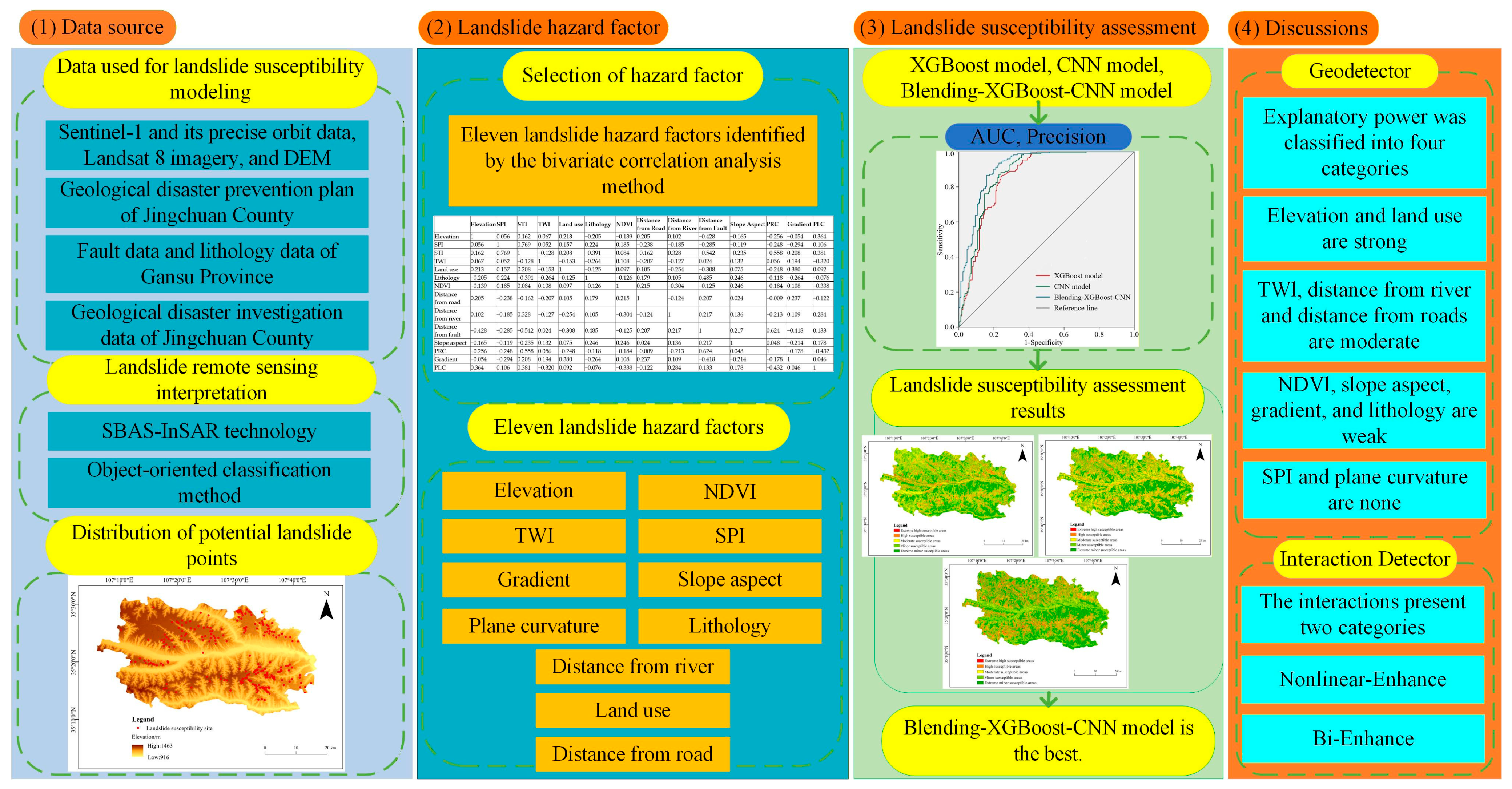
Figure 1. Research flowchart.
Applsci 15 11969 g001
Figure 2. Overview of the study area.
Applsci 15 11969 g002
Figure 3. Spatial baseline of image pairs.
Applsci 15 11969 g003
Figure 4. Temporal baseline of image pairs.
Applsci 15 11969 g004
Figure 5. Geocoding results.
Applsci 15 11969 g005
Figure 6. Average deformation rate.
Applsci 15 11969 g006
Figure 7. Multiscale segmentation results.
Applsci 15 11969 g007
Figure 8. Distribution of potential landslides.
Applsci 15 11969 g008
Figure 9. Hazard factor classification maps.
Applsci 15 11969 g009aApplsci 15 11969 g009b
Figure 10. Computational process of the XGBoost model.
Applsci 15 11969 g010
Figure 11. One-dimensional CNN network structure.
Applsci 15 11969 g011
Figure 12. ROC curves.
Applsci 15 11969 g012
Figure 13. Landslide susceptible zoning maps.
Applsci 15 11969 g013
Table 1. Data, download address and access date.
DataDownload AddressAccess Date
Sentinel-1 and its precise orbit datahttps://asf.alaska.edu/11 July 2024
Landsat 8 imageryhttps://www.usgs.gov/11 July 2024
Digital Elevation Model (DEM)https://envi.geoscene.cn/; https://geol.ckcest.cn/15 November 2024
Fault data of Gansu Provincehttps://geolckcest.cn/15 November 2024
Lithology data of Gansu Provincehttps://www.resdc.cn/9 December 2024
Geological disaster investigation data of Jingchuan Countyhttps://zrzy.pingliang.gov.cn/9 December 2024
Table 2. Rules for extracting potential landslides.
Feature ObjectNDVIGradientLayer 8GLCM Mean
Threshold range[0.1, 0.6][50°, 80°][430, 490][125, 129]
Table 3. Pearson correlation coefficient calculation results.
ElevationSPISTITWILand UseLithologyNDVIDistance from RoadDistance from RiverDistance from FaultSlope AspectPRCGradientPLC
Elevation10.0560.1620.0670.213−0.205−0.1390.2050.102−0.428−0.165−0.256−0.0540.364
SPI0.05610.7690.0520.1570.2240.185−0.238−0.185−0.285−0.119−0.248−0.2940.106
STI0.1620.7691−0.1280.208−0.3910.084−0.1620.328−0.542−0.235−0.5580.2080.381
TWI0.0670.052−0.1281−0.153−0.2640.108−0.207−0.1270.0240.1320.0560.194−0.320
Land use0.2130.1570.208−0.1531−0.1250.0970.105−0.254−0.3080.075−0.2480.3800.092
Lithology−0.2050.224−0.391−0.264−0.1251−0.1260.1790.1050.4850.246−0.118−0.264−0.076
NDVI−0.1390.1850.0840.1080.097−0.12610.215−0.304−0.1250.246−0.1840.108−0.338
Distance from road0.205−0.238−0.162−0.2070.1050.1790.2151−0.1240.2070.024−0.0090.237−0.122
Distance from river0.102−0.1850.328−0.127−0.2540.105−0.304−0.12410.2170.136−0.2130.1090.284
Distance from fault−0.428−0.285−0.5420.024−0.3080.485−0.1250.2070.21710.2170.624−0.4180.133
Slope aspect−0.165−0.119−0.2350.1320.0750.2460.2460.0240.1360.21710.048−0.2140.178
PRC−0.256−0.248−0.5580.056−0.248−0.118−0.184−0.009−0.2130.6240.0481−0.178−0.432
Gradient−0.054−0.2940.2080.1940.380−0.2640.1080.2370.109−0.418−0.214−0.17810.046
PLC0.3640.1060.381−0.3200.092−0.076−0.338−0.1220.2840.1330.178−0.4320.0461
Table 4. Hazard factor classifications.
Hazard FactorClassification
QuantitativeElevation916–1054 m, 1054–1141 m, 1141–1222 m, 1222–1303 m, 1303–1463 m.
Gradient0–5.241519704°, 5.241519704–11.35662602°, 11.35662602–17.47173235°, 17.47173235–24.02363197°, 24.02363197–55.69114685°.
Distance from road0–0.003018867 km, 0.003018867–0.007003772 km, 0.007003772–0.011109431 km, 0.011109431–0.017026411 km, 0.017026411–0.030792445 km.
Distance from river0–0.016142896 km, 0.016142896–0.035069049 km, 0.035069049–0.057335112 km, 0.057335112–0.087394297 km, 0.087394297–0.141946152 km.
SPI−13.81551075–−6.94360159, −6.94360159–−2.231435308, −2.231435308–−0.16986256,
−0.16986256–2.382560842, 2.382560842–11.21787262.
TWI−6907.754882813–949.229515165, 949.229515165–2731.225976562, 2731.225976562–5080.22131204, 5080.22131204–8887.213752298, 8887.213752298–13,747.204101563.
NDVI0.043099999–0.508318836, 0.508318836–0.654637664, 0.654637664–0.755935314,
0.755935314–0.842225904, 0.842225904–0.999800026.
PLC−2.428134441–−0.32080935, −0.32080935–−0.10004196, −0.10004196–0.060516142,
0.060516142–0.281283533, 0.281283533–2.689655066.
QualitativeSlope aspectPlane, North, Northeast, East, Southeast, South, Southwest, West, Northwest.
LithologyNewly accumulated soil, Loessal soil, Dark loessal soil.
Land useArable land, Forest, Grassland, Shrub land, Wetland, Water body, Artificial surface.
Table 5. AUC-related statistical values.
ModelAUCStandard ErrorAsymptotic SignificanceApproaching the 95% Confidence Interval
Lower LimitLimit
XGBoost model0.8820.0210.0000.8140.898
CNN model0.9000.0170.0000.8620.941
Blending-XGBoost-CNN model0.9120.0160.0000.8830.947
Table 6. Explanatory power of hazard factors on landslide susceptibility.
Hazard FactorElevationNDVITWISlope AspectGradient
q0.4510.6040.2040.4320.742
Hazard factorPLCDistance from riverDistance from roadLithologyLand use
q0.0790.3490.0450.1980.384
Table 7. Interaction detection results among hazard factors.
ElevationNDVITWISlope AspectGradientPLCDistance from RiverDistance from RoadLithologyLand Use
Elevation0.416NENENENENENENENENE
NDVI0.1200.894NEBENEBENENENENE
TWI0.8940.3170.894NENENENENEBENE
Slope aspect0.4890.0290.9160.415NEBEBENENENE
Gradient0.8590.3470.2470.1540.129NENENENENE
PLC0.132 0.0950.3790.8440.4510.045BEBEBENE
Distance from river0.9510.4840.2940.6260.1520.5620.207NEBENE
Distance from road0.4520.1820.3370.0520.4850.8790.3510.305BENE
Lithology0.5890.3080.6470.5890.8720.1560.5090.4290.117BE
Land use0.7840.5460.6530.2970.5460.4510.672 0.6040.694 0.462
Disclaimer/Publisher’s Note: The statements, opinions and data contained in all publications are solely those of the individual author(s) and contributor(s) and not of MDPI and/or the editor(s). MDPI and/or the editor(s) disclaim responsibility for any injury to people or property resulting from any ideas, methods, instructions or products referred to in the content.