A Review of the CLH Index, an Empirical Methodology for TBM Cutter Wear Estimation

Abstract

This study presents a comprehensive review of the CLH index, a predictive tool developed to estimate the wear of tunnel boring machine (TBM) disc cutters operating in hard rock conditions. The CLH index provides a simplified, time-efficient, and cost-effective alternative to conventional wear prediction methods by employing a statistically derived empirical formula. The methodology is based on the identification and quantitative assessment of key rock properties that influence cutter wear. A detailed statistical analysis was conducted to validate the index, quantify potential errors, and determine confidence levels. As part of this review, updated reference tables are proposed to facilitate cutter wear estimation without the need for preliminary laboratory testing. These tables are derived from empirical data obtained at the Rock Mechanics Laboratory of the Higher Technical School of Mining and Energy Engineers (ETSIME-UPM), using operational records from TBM excavation in multiple Spanish high-speed railway tunnels, with a total length exceeding 120 km. The results confirm the reliability and practical applicability of the CLH index as a decision-support tool in TBM performance forecasting and maintenance planning.

1. Introduction

The growth in underground construction, driven by societal demand for better communications and environmental constraints, has enabled the development of large tunnel boring machines (TBMs) for the construction of a larger number of tunnels and for more efficient excavation of heterogeneous terrain.

Tunnel boring machines (TBMs) have become essential tools in the construction of modern underground infrastructure due to their ability to perform continuous excavation, enhance operational safety, and reduce environmental impact compared to conventional methods. Their widespread adoption in large-scale projects, such as high-speed railway lines and urban metro systems, has been driven by advances in automation, cutterhead design, and ground conditioning technologies. Nevertheless, optimal TBM performance is highly dependent on site-specific geotechnical conditions, with rock abrasivity being one of the most critical factors, as it directly affects cutter wear, advance rates, and overall project costs.

Among the various operational parameters, cutter wear is one of the most difficult to predict due to the complex and dynamic interaction between the cutting tools and the ground. This interaction is influenced by multiple factors, including rock mineralogy, grain size, uniaxial compressive strength, and the presence of discontinuities. Cutter wear not only impacts the excavation rate but also contributes significantly to unplanned stoppages, maintenance costs, and operational risks. Therefore, accurate estimation of cutter consumption is essential for improving TBM utilization and minimizing downtime.

The aim of this article is to reduce the complexity of predicting TBM cutter wear, as the large number of parameters involved in predicting the progress of this type of TBM makes its calculation extremely complicated.

The index presented in this article is not intended to replace these existing methods but to act as an additional tool, offering simplicity and low testing costs, making it especially suitable for preliminary design phases. The six-parameter structure enables the CLH to encompass rock mass variability and heterogeneity, providing a more comprehensive view. The re-vision presented in this study demonstrates greater robustness and accuracy in cutter wear time estimation.

The TBM utilization factor U is a key performance indicator, defined as the ratio between the net advance rate Ar (excluding stoppages) and the penetration rate Pr (including stoppages), as expressed in Equation (1):

$$U \left(\%\right)={\displaystyle \frac{P_r}{A_r}}\times 100$$

(1)

Typical values of U range between 30% and 50% [1]. Stoppages may be planned (e.g., scheduled maintenance, tool inspection) or unplanned (e.g., cutter failure, ground instability), and minimizing the latter requires a strong focus on preventive maintenance and robust predictive models [2,3].

Over the past decades, numerous models have been proposed to estimate cutter life and penetration rates, many of which rely on quantifying rock abrasivity through standardized tests such as the Cerchar Abrasivity Index (CAI), the LCPC abrasivity test, and the Sievers’ J-value [4,5,6]. While these models have provided valuable insights, they often exhibit limited applicability outside the specific geological contexts for which they were developed. Moreover, many have been calibrated exclusively for rock excavation, despite the increasing use of TBMs in mixed-face conditions, where soil and rock coexist within the same section [4,7].

The technological evolution of TBMs has expanded their use to a wider range of geological environments, complicating machine selection and performance prediction. Engineers must consider not only lithological variability but also operational constraints, cutterhead configuration, and real-time monitoring data. Despite the availability of empirical and semi-empirical models [2,8,9,10], considerable uncertainty remains in their predictive capability, particularly in heterogeneous and abrasive rock masses [6].

In this context, the present study aims to contribute to the field by developing a new empirical approach for estimating cutter life, based on laboratory data and field observations. The research is grounded in rock samples collected along more than 120 km of high-speed railway tunnels in Spain, including the following:

• Guadarrama Tunnels (Madrid–Segovia): Two parallel tubes, 9.5 m in diameter, 28 km in length.
• Das Maceiras Tunnels (Pontevedra): Two parallel tubes, 9.5 m in diameter, 8.5 km in length.
• Pajares Tunnels (León–Asturias): Two parallel tubes, 9.5 m in diameter, 24.6 km in length.

These samples were tested at the Rock Mechanics Laboratory of the Higher Technical School of Mining and Energy Engineers (ETSIME-UPM), using a comprehensive suite of geomechanical tests to characterize rock properties and monitor TBM performance. The resulting dataset enabled the development of an empirical formula to estimate the average service life of cutterhead disc cutters, based on a newly proposed index referred to as CLH. It should be noted that “CLH” is not an acronym, but rather a simple label chosen by the authors to represent the model.

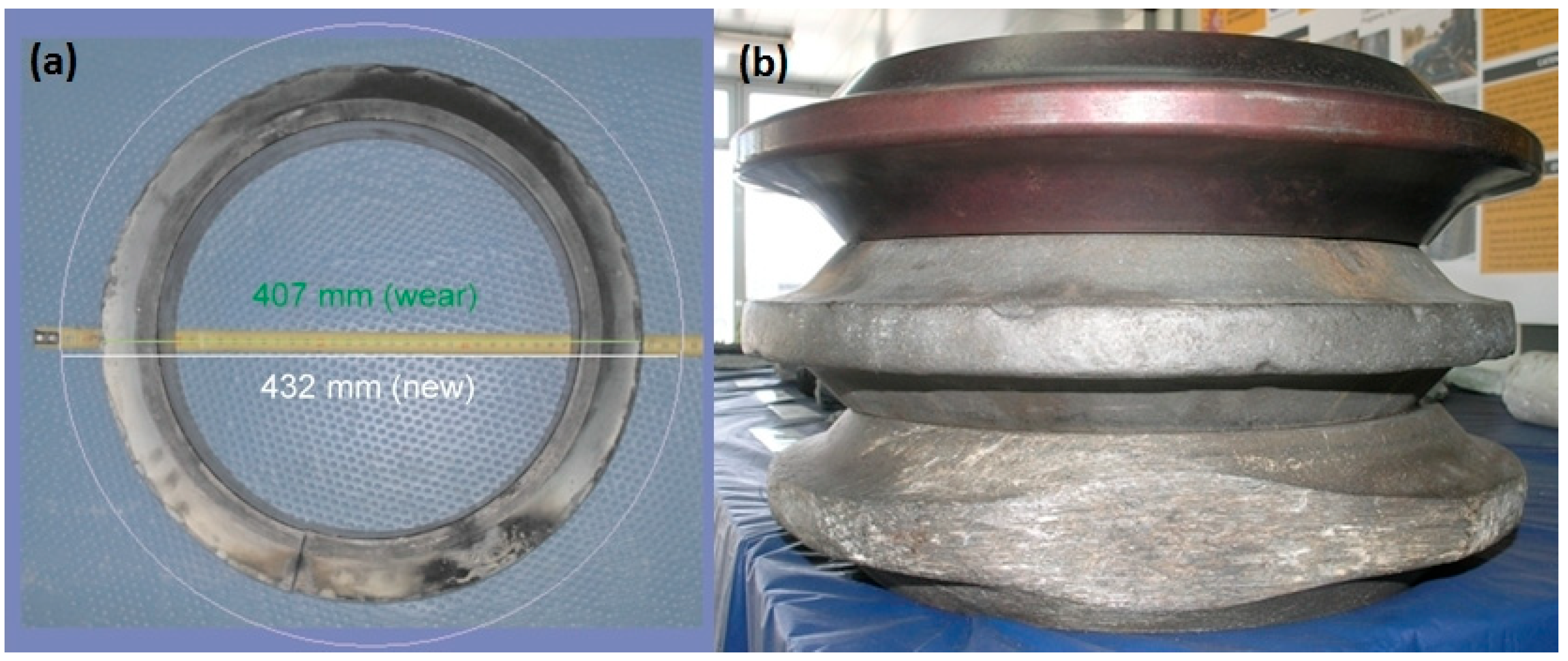
In hard and abrasive rock masses, cutter replacement costs can represent a significant portion of total excavation expenses. As illustrated in Figure 1a [11], the wear of a 17″ (432 mm) disc cutter used in the Guadarrama Tunnels exemplifies the impact of sustained contact with abrasive rock. Although TBMs can bore through most natural rock masses, execution costs may become prohibitively high compared to drill-and-blast methods [12]. As shown in Figure 1b, cutter replacement may be required due to various factors, including bearing seizure, ring breakage, or wear from prolonged rock contact.

In the Guadarrama Tunnels, wear was identified as the predominant cause of cutter consumption, accounting for 80% and 65% of replacements in the two tubes, respectively [11]. The main causes of cutter replacement observed in the studied projects include the following:

• Wear of the cutter ring during face excavation
• Breakage of the ring support due to rockfall
• Misalignment of the cutter ring relative to its axis
• Accelerated wear of peripheral cutters due to longer travel paths
• Loss of bearing lubrication and bearing seizure or fracture
• Heterogeneous face conditions and abrupt geological transitions
• Fracturing of the excavation face leading to rock block falls or jamming
• Excessive torque or thrust resulting in peak loads on individual cutters
• Elevated vibration levels and insufficient water flow for cutterhead cooling

Cutter-related stoppages recorded in the Guadarrama Tunnels included cutterhead inspection and verification, cutterhead cleaning, cutter tightening, overcutting for gauge cutter installation, cutter replacement, retaining ring welding, and wedge-related cutter repairs. It is worth noting that some stoppages unrelated to cutter issues were opportunistically used for cutter maintenance or replacement.

By integrating laboratory data, field observations, and operational records, this study proposes a new predictive framework for estimating cutter life, with the aim of improving TBM performance forecasting, reducing maintenance costs, and supporting more efficient excavation in abrasive geological conditions.

The application of the CLH index in multiple Spanish high-speed railway tunnels relies on original datasets compiled for this study from internal technical reports prepared for the joint ventures (UTEs) of the Guadarrama, Das Maceiras, and Pajares tunnels. These reports provided Sievers’ J (SJ), S20, AVS, equivalent quartz content, UCS, and CAI results, together with detailed TBM operation and cutter-consumption records.

2. Materials and Methods

Numerous empirical and analytical models have addressed TBM performance and cost prediction, including penetration rates, cutter wear, and project timelines [7,13,14,15,16,17]. Among the most widely accepted methods are: (i) the Norwegian Method (developed at the Norwegian University of Science and Technology, NTNU) [15], developed by the Norwegian Institute of Technology; (ii) the Colorado School of Mines Method (CSM) [18]; (iii) the Rock Mass Excavability Index (RME) developed by Barton [19]; and (iv) the QTBM method proposed by Bieniawski [20]. While these methods have been applied successfully in various tunnelling projects, each presents limitations when applied to specific geological settings or mixed-face conditions, thereby motivating the development of alternative predictive tools such as the CLH index [21,22].

The NTNU method is based on performance data collected from TBMs operating in a range of rock types, enabling the estimation of cutter wear, penetration rates, and tunnelling times. It accounts for both intact rock properties, using the Drilling Rate Index (DRI), and rock mass characteristics. Originally developed for predicting the penetration rate of percussive drilling hammers, the DRI is now widely regarded as a reliable indicator of TBM advance rates.

The CSM method assesses the influence of rock mechanical properties on TBM cutting performance by determining cutter forces, from which thrust, torque, and cutterhead power are calculated. These calculated parameters are compared against the machine’s design specifications to determine the maximum achievable penetration rate or to verify a target rate.

The QTBM method adapts Barton’s Q-system for rock mass classification to predict TBM net advance rates. It integrates parameters such as joint spacing, rock quality designation, groundwater conditions, and stress factors.

The RME method proposed by Bieniawski incorporates five key parameters describing rock mass behaviour and TBM characteristics to derive an index for predicting excavability. While useful in preliminary feasibility studies, it requires calibration for each geological setting.

2.1. Development of the CLH Index

The CLH index was developed at the ETSIME-UPM Rock Mechanics Laboratory to provide a simple, rapid, and cost-effective method for estimating TBM disc cutter life in hard rock tunnelling. The methodology is underpinned by extensive laboratory testing and statistical analysis of rock samples from over 120 km of TBM-excavated Spanish high-speed railway tunnels, including the Guadarrama, Das Maceiras, and Pajares projects.

A total of 204 samples, representing various lithologies such as orthogneiss, cataclasites, porphyry, and granite, were collected for testing. All laboratory investigations were performed at the ETSIME-UPM Rock Mechanics Laboratory, equipped with calibrated instruments and testing systems compliant with International Society for Rock Mechanics (ISRM) suggested methods, as well as ASTM and UNE standards where applicable. Procedures were designed to ensure repeatability, comparability, and statistical reliability of results.

Rock samples were collected during core drilling campaigns conducted alongside tunnel excavation. Each specimen was labelled with precise geological and spatial provenance to enable correlation with in situ TBM performance data. Prior to testing, samples were cleaned, dried, and, where required, cut to standardized dimensions. Test sequences were planned to minimize alteration of material properties between procedures. Duplicate or triplicate specimens were tested to assess variability, and anomalous results were re-tested. All results were stored in a centralized database for subsequent calibration of the CLH index.

Six rock properties were identified as the most influential on cutter wear and service life, and were determined using the following standardized laboratory procedures:

• Drillability (Sievers’ J miniature drill test, SJ). Quantifies the ease of rock penetration by a steel stylus under controlled conditions. A conical steel point is applied to the rock surface under a specified load, and penetration depth is recorded after a fixed number of revolutions. Lower SJ values indicate harder, less drillable rocks, whereas higher values correspond to softer, more easily drillable lithologies. Drillability influences cutter penetration rate and the energy required for excavation [23,24].
• Brittleness (Impact test, S20). Measures the tendency of a rock to fracture upon impact. Standardized specimens are subjected to repeated blows from a falling weight, and the resulting grain size distribution is analyzed. Higher S20 values reflect greater brittleness, often linked to increased cutter wear due to sharp-edged fragments accelerating tool degradation [15,25].
• Rock abrasivity (Abrasion Value Steel, AVS). Evaluates the abrasive effect of rock particles on steel. Rock material, ground to a standardized grain size, is used to abrade a steel specimen under controlled conditions. The weight loss of the steel piece is recorded as the AVS value, with higher values indicating greater potential for cutter ring wear during TBM operation [26].
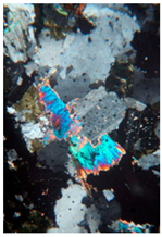
• Equivalent quartz content. Determined petrographically from thin sections under a polarizing microscope. The Rosiwal method is used to quantify mineral content and relative hardness, yielding an equivalent quartz percentage. Higher quartz content typically correlates with increased abrasivity and reduced cutter wear [27,28].
• Uniaxial compressive strength (UCS). Represents the maximum axial stress a rock specimen can withstand before failure. Tests are carried out on cylindrical cores (commonly 54 mm diameter) at a constant strain rate until failure. Higher UCS values require greater TBM thrust force for penetration, increasing cutter loading and wear [29,30].
• Cerchar Abrasivity Index (CAI). Quantifies rock abrasivity by scratching the rock surface with a steel stylus under a specified load (typically 70 N) over a fixed length. The width of the wear flat on the stylus tip is measured; higher CAI values indicate greater abrasivity and a higher likelihood of accelerated cutter-ring wear [31].

2.2. CLH Index Calculation and Validation

From all the samples evaluated in the ETSIME-UPM Rock Mechanics Laboratory for monitoring various TBM-excavated tunnels in Spain, 204 were selected. These samples had in common the six necessary tests for the calculation of the CLH index. The index is derived from a multivariate statistical correlation between these key rock properties and in-situ measurements of TBM cutter wear.

The data analyzed in Section 2.2 and Section 2.3 were obtained from internal technical reports prepared for the joint ventures (UTEs) responsible for the Guadarrama, Das Maceiras, and Pajares tunnels and were made available to the authors through collaboration agreements.

The CLH index is calculated using the following empirical Equation (2):

$$CLH=A+B+C+D+E+F$$

(2)

where

• A is the numerical value assigned to drillability (SJ).
• B is the numerical value assigned to brittleness (S20).
• C is the numerical value assigned to rock abrasivity on steel (AVS).
• D is the numerical value assigned to equivalent quartz content.
• E is the numerical value assigned to uniaxial compressive strength (UCS).
• F is the numerical value assigned to the Cerchar Abrasivity Index (CAI).

Each of the six test results is mapped to a specific numerical score (

Table 1. Assignment of values for the six parameters considered in the determination of the CLH index.

SJ (1/10 mm)	A	S20 (%)	B	AVS (mg)	C	Qz (%)	D	CS (MPa)	E	CAI	F
<10	4	0–20	3	0–10	10	0–10	20	0–25	10	<0.5	10
10–20	10	20–30	4.5	10–15	9	11–20	19	25–50	9.5	0.5–1	9
20–30	16	30–35	5	15–20	8	21–25	18	50–75	9	1–2	8
30–40	21	35–40	5.5	20–25	8.5	25–30	17	75–100	8.5	2–3	7
40–50	26	40–45	6	25–30	7.5	30–35	16	100–125	8	3–4	6
50–60	31	45–50	6.5	30–35	7	35–40	15	125–150	7.5	4–5	5
60–70	35	50–55	7	35–40	6.5	40–45	14	150–175	7	5–6	4
>70	40	55–60	7.5	40–45	6	45–50	13	175–200	6.5	6–7	3
		60–65	8	45–50	5.5	50–55	12	200–225	6	7–8	2
		65–70	8.5	>50	5	55–60	11	225–250	5.5	>8	1
		70–75	9			60–65	10	250–275	5
		75–80	9.5			65–70	9	275–300	4.5
		>80	10			70–100	3	300–325	4
								325–350	3.5
								>350	3

). These scores were determined empirically through iterative calibration to align, as closely as possible, with the observed service life of the complete set of cutters on the TBM cutterhead. Consequently, the CLH index ranges from 19 to 100, with higher index values indicating a longer expected cutter wear. Figure 2 illustrates the direct relationship between the CLH index and cutter wear, showing that higher index values correspond to longer observed service life for TBM disc cutters.

2.3. Statistical Analysis

As noted in Section 2.2, the dataset derives from internal UTE technical reports covering TBM operation, cutter consumption, and geomechanical testing. Analysis of variance (ANOVA) assessed the statistical significance of each predictor, with p-values below 0.05 indicating a meaningful contribution. Ninety-five percent confidence intervals were computed for all regression coefficients to evaluate their stability and precision.

Outliers and influential observations were identified using Cook’s distance and leverage statistics and were reviewed to distinguish genuine extreme cases from measurement or recording anomalies. Model robustness was further evaluated through cross-validation by partitioning the dataset into training and testing subsets to assess predictive performance.

This statistical framework provided a quantitative measure of the CLH index’s reliability and highlighted the relative importance of each rock property in influencing TBM cutter wear. The coefficient of determination (R²) is used to evaluate the goodness of fit of the regression models developed in this study. R² measures the proportion of the variance in the dependent variable that is predictable from the independent variable. Higher R² values indicate a stronger correlation between the predicted and observed data, and thus a more reliable model.

3. Results and Discussion

This section presents and analyses the key findings from the application and review of the CLH index. It begins with a detailed examination of results for a representative sample to illustrate the methodology and computed values. A global comparative analysis then synthesises behaviours observed across all samples and highlights significant statistical correlations. Finally, the implications for tunnelling engineering are discussed, along with potential avenues for improving the index.

3.1. Detailed Characterisation of the Reference Sample (Biotite Granite)

Table 2. Averages obtained for each of the lithologies present in the study.

Number of Samples	Lithology According to Petrographic Study	SJ (1/10 mm)	S20 (%)	AVS	Quartz Equivalent Content (%)	CS (MPa)	CAI
14	Cataclastic granite	27.44	45.69	31.89	28.45	55.26	2.15
9	Pink granite	19.29	52.56	34.88	31.5	71.3	2.15
10	Two-mica granite	26.39	44.69	36.24	48.19	82.76	2.76
12	Porphyry	13.51	42.15	28.52	35.25	151.54	2.25
15	Porphyritic biotite granite	25.52	49.11	33.22	45.99	58.08	2.65
44	Biotite granite	23.15	49.28	35.59	45.05	155.85	2.84
25	Biotite gneiss	18.93	44.95	35.27	47.68	60.11	2.84
28	Orthogneiss	13.5	33.33	34.02	58.8	234.85	3.64
6	Microgranite	17.6	44.81	37.61	56.72	88.31	3
6	Biotite granodiorite	53.55	49.18	34.45	46	66.71	3.02
5	Amphibolic quartz diorite	18	34.88	24.67	41.16	77.41	2.35
3	Amphibolic quartz diorite	36.5	29.94	8.33	35.72	250.6	2.97
4	Feldspathic hornfels with diopside	15.82	41.27	22.5	47.05	132	2.84
5	Gabbro diorite	32.12	35.71	10.33	31.9	367.75	2.28
10	Dolomitic marble	88.76	45.84	5.07	9.14	159.32	1.25
8	Biotite orthogneiss	37.33	47.71	25.38	47.23	192	3.79

provides the lithological descriptions and identifiers for the 204 analyzed samples, offering the geological context for the subsequent laboratory testing.

Six fundamental laboratory tests were performed to determine the CLH index. Sievers’ J (SJ) test results, which measure indentation resistance, are shown in

Table 3. Results of the Sievers’ J (SJ) test for Sample No. 1.

Sample No. 1
Lithology		Biotite Granite
Test	Value	Units
1	2.3	mm
2	2.5	mm
3	2.8	mm
4	2.7	mm
Average	2.575	mm
SJ	25.75	1/10 mm

. The S20 test, evaluating resistance to repeated impact crushing, is summarized in

Table 4. Results of the brittleness (S20) test for Sample No. 1.

Sample No. 1
Lithology	Biotite Granite
Test	1st Mass (g)	2nd Mass (g) (1)	Difference (%)
1	501.0	159.6	31.86
2	500.9	174.1	34.76
3	499.1	186.4	37.35
Average S20 (%)			34.66

⁽¹⁾ Mass passing through the 11.2 mm sieve.

. Abrasion Value on Steel (AVS) results, quantifying mass loss on steel due to rock dust abrasion, are presented in

Table 5. Results of the abrasivity to steel (AVS) test for Sample No. 1.

Sample No. 1
Lithology	Biotite Granite
Test	Weight Before (g)	Weight After (g)	Weight Loss (mg)
1	25.489	25.454	35.00
2	25.345	25.313	32.00
Average AVS (mg)			33.50

. Equivalent quartz content, determined from thin-section microscopy and Rosiwal hardness factors, is reported in

Table 6. Determination of Equivalent Quartz Content.

Sample No. 1
Lithology	Biotite Granite
Mineral	Mineral Cont. (Fraction)	Rosiwall Factor	Qz (%)
Quartz	0.31	100	31
Potassium feldspar	0.29	35	10.15
Plagioclase	0.14	35	4.9
Biotite	0.13	4	0.52
Opaques	0.02	50	1
		Total	47.57

. Uniaxial compressive strength (UCS) results are presented in

Table 7. Results of the Uniaxial Compressive Strength Test for Sample No. 1.

Sample No. 1
Lithology	Biotite Granite
Diameter	61.6	mm
Height	157.0	mm
Failure load	171.9	MPa
Poisson’s ratio	0.262
Young’s modulus	57.956	GPa

. Finally, Cerchar Abrasivity Index (CAI) results, estimating rock abrasivity from the wear flat produced on a steel stylus after repeated scratching, are given in

Table 8. Results of the Cerchar Abrasivity Index (CAI) Test for Sample No. 1.

Sample No. 1
Lithology				Biotite Granite
Microscope Reading
1	2	3	4	5	Average	Wear (mm)	CAI
10	9	7	10	8	8.8	0.2904	2.904

.

The CLH index was calculated by summing the values assigned to each parameter according to the scoring system defined in Table 1 of the original methodology, as expressed in Equation (2).

For the biotite granite sample, the assigned scores yielded a CLH index of 55, which lies within the mid-range of values observed in this study (19–100). The detailed correspondence between measured parameters, assigned scores, and the final index value is summarized in Table 8. Using Equation (2), which defines a linear relationship between the CLH index and cutter wear, this value predicts a cutter life of 94.52 h. The prediction differs by 5.25% from the observed 89.81 h, a deviation well within the study’s acceptable error range. Although no direct comparison with other specific samples is presented here, this reference sample is incorporated into the overall statistical analysis of the full dataset.

Table 9. Calculation of the CLH Index for Sample No. 1.

SJ (1/10 mm)	A	S20 (%)	B	AVS	C	Equivalent Quartz (%)	D	UCS (MPa)	E	CAI	F	CLH Index
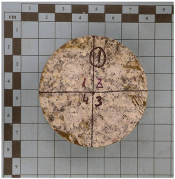
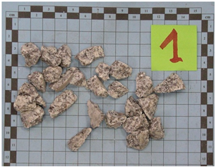
25.75	16	34.66	5	33.50	7	47.57	13	171.9	7	2.90	7	55

presents the calculation of the CLH Index for Sample No. 1, which is incorporated into the overall statistical analysis of the full dataset.

3.2. Comprehensive Comparative Analysis

This section presents a consolidated overview of the results obtained from the analysis of all rock samples used in the study. It explores the overall distribution of CLH index values, identifies statistically significant correlations with the actual wear rate, and contrasts the performance of the CLH with other existing predictive methods. Finally, it addresses the validation and practical applicability of this index in various geological scenarios.

3.2.1. Distribution of CLH Values

The study encompassed 204 rock samples collected from Spanish railway tunnels excavated using TBMs. Predominant lithologies included igneous and metamorphic rocks such as orthogneiss, cataclasites, porphyries, and several granites (biotite, pink, two-mica, porphyritic biotite), as well as biotite gneiss, microgranite. biotite granodiorite, amphibolic quartz diorite, Amphibolic quartz diorite, feldspathic hornfels with diopside, gabbro-diorite, and dolomitic marble.

The average CLH index values, calculated for each of these lithologies based on the six measured parameters, showed significant variability. For example, orthogneiss presented a CLH of 45 (considered low), whereas dolomitic marble reached a CLH of 92 (indicating a considerably high level of abrasivity and expected wear). Biotite granodiorite scored 73. Other rock types, such as granites, gneiss, and porphyries, were found within intermediate ranges, generally between 52 and 63. This distribution suggests that the CLH index is sensitive to the varying geomechanical and mineralogical properties of the rocks.

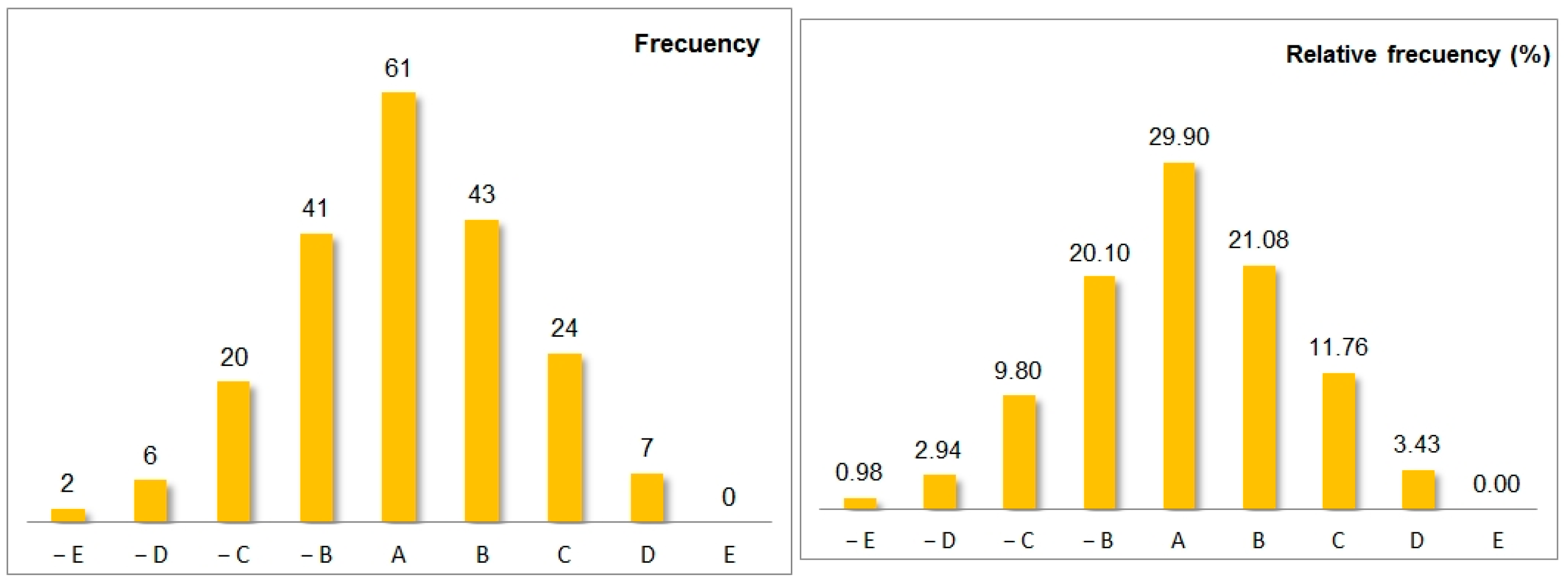
The distribution of errors obtained when estimating cutter life using the CLH index reveals that an impressive 92.65% of the 204 samples studied exhibited a prediction error equal to or below 12.5% (encompassing Classes A, B, and C). More specifically, 29.90% of the samples were classified in Class A, with very low errors within ±2.5%. The frequency and relative frequency graphs of this error distribution are shown in Figure 3.

3.2.2. Statistically Significant Correlations

To validate the predictive capability of the CLH index, a comprehensive statistical analysis examined the relationship between the CLH index (independent variable, (X) and actual cutter wear (dependent variable, (Y). The sample covariance (S_xy) was 109.84, a positive value indicating a direct relationship: as the CLH index increases, cutter wear tends to increase. This interpretation is consistent with the original study. The sample covariance is computed using Equation (3):

$$S_{xy}={\displaystyle \frac{{\sum }_{i=1}^n\left(x_i-\overline{X}\right)\cdot \left(y_i-\overline{Y}\right)}{n-1}}$$

(3)

where $x_i$ and $y_i$ are the i-th values of variables X and Y, respectively, $\overline{X}$ is the sample mean of $X$, $\overline{Y}$ is the sample mean of Y. The sample mean is calculated according to Equation (4):

$$\overline{X}={\displaystyle \frac{x_1+x_2+x_3+\cdot \cdot \cdot +x_n}{n}}={\displaystyle \frac{{\sum }_{i=1}^n{x}_i}{n}}$$

(4)

The calculations using these expressions yielded the following results:

$$\overline{X}=53.29, \overline{Y}=91.59, { S}_{xy}=109.84$$

The Pearson correlation coefficient (R), calculated using Equation (5) in combination with Equation (6) (Sample Standard Deviation), was 0.929. This value, extremely close to 1, demonstrates an extraordinarily strong linear relationship between the CLH index and the actual cutter life. This correlation is even higher than in the original CLH index version (R = 0.916). The Pearson correlation coefficient is defined as:

$$R={\displaystyle \frac{S_{xy}}{S_x\cdot S_y}}$$

(5)

where $S_{xy}$ is the sample covariance between variables X and Y, and $S_x$ and $S_y$ are the sample standard deviations of X and Y, respectively. The sample standard deviation is calculated according to Equation (6):

$$S_x=\sqrt{{\displaystyle \frac{{\sum }_{i=1}^n{\left(x_i-\overline{X}\right)}^2}{n-1}}}$$

(6)

Analogously, $S_y$ is obtained by replacing $x_i$ with $y_i$ and $\overline{X}$ with $\overline{Y}$. Applying these expressions yielded the following results:

$$S_x=8.77, S_y=17.75, R=0.929$$

The coefficient of determination (R²), which measures the proportion of the variance in the dependent variable that is predictable from the independent variable, was 0.8635. A value so close to 1 indicates that the CLH index is a very strong determinant in explaining actual cutter life.

The fitted linear relationship is shown in Figure 4 and is expressed in Equation (7):

$$y=1.846\cdot CLH-7.0101$$

(7)

where:

• Y = Actual cutter life (hours)
• CLH = CLH Index

For example, for a CLH of 55, the calculated cutter life is 94.52 h, representing a deviation of only 5.25% from the observed value of 89.81.

The six parameters selected, drillability, brittleness, rock abrasivity, quartz equivalent content, uniaxial compressive strength, and Cerchar abrasivity index, were carefully chosen due to their well-documented and significant influence on cutter wear and service life. While the study does not aim to quantify the individual contribution of each parameter within the overall CLH correlation, their combined inclusion is considered a core strength of the method. By integrating multiple key factors, the CLH index adopts a technically sound approach that reduces dispersion, aligns closely with a normal distribution, and enhances the robustness and predictive reliability of the model.

3.2.3. Validation and Applicability of the CLH Index

The validation of the CLH index is supported by a robust regression analysis showing a strong linear relationship between the CLH index and actual cutter wear, with a coefficient of determination (R²) of 0.8635. This goodness-of-fit is reflected in the error distribution: 92.65% of the 204 samples exhibited a prediction error at or below 12.5% (Classes A, B, and C combined), indicating high accuracy in most cases. Furthermore, the normal distribution analysis (Gauss–Laplace curve) indicated an 83.72% probability that the error falls within ±10%, confirming that CLH estimates are highly likely to remain within an acceptable tolerance. This numerical reliability is summarized in

Table 10. Probabilities within an error range.

X	Z	F(Z) %	Probability %
2.50	0.23	59.09	27.17
−2.50	−0.47	31.92
5.00	0.58	71.90	51.29
−5.00	−0.82	20.61
7.50	0.93	82.38	70.28
−7.50	−1.17	12.10
10.00	1.29	90.15	83.72
−10.00	−1.52	6.43
12.50	1.64	94.95	91.88
−12.50	−1.87	3.07
15.00	1.99	97.67	96.35
−15.00	−2.22	1.32

, which presents the probability of prediction errors falling within different tolerance ranges.

To characterize the distribution of errors, the probability density and cumulative probability functions for both the original and standardized variables (x and Z) are presented in Equations (8)–(12). These functions describe the likelihood of prediction errors occurring within a given range, under the assumption of a normal distribution.

The probability density function for the normal distribution is defined in Equation (8):

$$f(x)={\displaystyle \frac{1}{\sigma \sqrt{2\pi }}}\cdot e^{-{\displaystyle \frac{{\left(x-\mu \right)}^2}{2{\sigma }^2}}}$$

(8)

where:

• $f\left(x\right)$= probability density of variable x
• x = value of the variable
• $\mu$ = population mean (μ = −0.83)
• σ = population standard deviation (σ = 7.1301)

The corresponding cumulative probability function is given in Equation (9):

$$F(x)={\int }_{-\infty }^x{\displaystyle \frac{1}{\sigma \sqrt{2\pi }}}{e}^{-{\displaystyle \frac{{\left(x-\mu \right)}^2}{2{\sigma }^2}}}dx$$

(9)

The standardized form of the variable X is calculated using Equation (10):

$$Z={\displaystyle \frac{X-\mu }{\sigma }}$$

(10)

The probability density function for the standardized variable Z is defined in Equation (11):

$$f(z)={\displaystyle \frac{1}{\sqrt{2\pi }}}{e}^{-{\displaystyle \frac{z^2}{2}}}$$

(11)

Finally, the cumulative probability function for the standardized variable Z is expressed in Equation (12):

$$F(z)={\displaystyle \frac{1}{\sqrt{2\pi llev}}}{\int }_{-\infty }^z{e}^{-{\displaystyle \frac{z^2}{2}}}dz$$

(12)

The lithology-specific CLH index values obtained in this study are summarized in

Table 11. CLH Index for different rock types.

Number of Samples	Lithology According to Petrographic Study	A	B	C	D	E	F	CLH Index
14	Cataclastic granite	16	6.5	7	17	9	7	63
9	Pink granite	10	7	7	16	9	7	56
10	Two-mica granite	16	6	6.5	13	8.5	7	57
12	Porphyry	10	6	7.5	15	7	7	53
15	Porphyritic biotite granite	16	6.5	7	13	9	7	59
44	Biotite granite	16	6.5	6.5	13	7	7	56
25	Biotite gneiss	10	6	6.5	13	9	7	52
28	Orthogneiss	10	5	7	11	5.5	6	45
6	Microgranite	10	6	6.5	11	8.5	7	49
6	Biotite granodiorite	31	6.5	7	13	9	6	73
5	Amphibolic quartz diorite	10	5	8	14	8.5	7	53
3	Amphibolic quartz diorite	21	4.5	10	15	5	7	63
4	Feldspathic hornfels with diopside	10	6	8	13	7.5	7	52
5	Gabbro diorite	21	5.5	9	16	3	7	62
10	Dolomitic marble	40	6.5	10	20	7	8	92
8	Biotite orthogneiss	21	6.5	7.5	13	6.5	6	61

. These tables provide valuable reference values for preliminary estimations in similar geological contexts. However, as noted in the study, they should be interpreted with due caution, primarily because of the limited number of samples available for certain lithologies, which may result in significant deviations in average values.

Overall, the validation process confirms that the CLH index is a highly reliable predictive tool for estimating cutter wear and life in TBM tunnelling. Its integration of six key rock parameters—drillability, brittleness, rock abrasivity, equivalent quartz content, uniaxial compressive strength, and Cerchar abrasivity index—ensures a comprehensive characterisation of rock mass behaviour. This makes it particularly suitable for application in preliminary project phases, offering both technical robustness and cost-efficiency compared to more complex predictive models.

3.3. General Discussion

The improved robustness and accuracy of the CLH index support its use during the preliminary stages of projects, providing a global and sufficiently precise estimation of excavation performance. One direct implication of more accurate service-life estimation is a more precise assessment of cutter replacement costs, which contributes significantly to more reliable operational expenditure (OPEX) forecasts.

As a simple and economical method, the CLH index enables early assessment of potential cutter wear, supporting better resource management. Although the document does not detail the selection of cutting parameters, prior knowledge of expected wear is fundamental for optimizing preventive maintenance strategies and planning machine stoppages for tool changes more efficiently, thereby minimizing downtime and improving utilisation rates.

Future work should expand the number of tests for each rock type, particularly for lithologies with limited sample counts. Expanding this database is crucial for validating and refining the lithology-specific CLH tables, thereby improving statistical reliability and reducing observed deviations.

Furthermore, the multifactorial nature of the CLH index, incorporating six parameters to capture rock-mass variability, opens avenues for research into parameter weighting and the inclusion of additional factors to address more complex geological conditions and specific excavation scenarios, while maintaining its role as a complementary tool rather than a replacement for other methodologies.

4. Conclusions

This study introduces an updated and refined version of the CLH index, providing a reliable and efficient approach for predicting TBM cutter wear in tunnelling projects. By integrating six key rock-related parameters, the index captures geological variability while maintaining simplicity and cost-effectiveness. The main findings are as follows.

• Broad applicability in tunnelling projects: The CLH index serves as a complementary tool, enhancing cutter service-life estimation without replacing existing predictive methods.
• Incorporation of multiple parameters: The methodology uses six parameters directly linked to cutter wear (drillability, brittleness, rock abrasivity, equivalent quartz content, uniaxial compressive strength, and the Cerchar abrasivity index), capturing rock mass variability and heterogeneity.
• Cost-effectiveness and simplicity: The required tests are simple and low-cost, making the method well-suited to preliminary project stages.
• Improved robustness and accuracy: The revised CLH index shows higher reliability and precision in estimating cutter wear than earlier versions, as supported by statistical analysis.
• Quantifiable operational benefits: More accurate wear predictions enable better estimation of cutter replacement costs, improving OPEX calculations for the overall project.
• Statistical consistency: The relationship between the CLH index and cutter wear follows a normal distribution, enabling probabilistic analysis of wear predictions.
• Technical advantage of a multi-parameter design: Including six key parameters reduces result dispersion and improves predictive reliability, providing a more robust planning tool.
• Streamlined formulation: After evaluating several analytical formulations, the six selected parameters produced sufficiently close to target performance while keeping the calculation as simple as possible.
• In sum, the updated CLH index delivers a practical, data-driven framework that couples geological realism with methodological simplicity, enabling more reliable planning, cost control, and risk reduction for hard-rock TBM projects.

References

1. Sapigni, M.; Berti, M.; Bethaz, E.; Busillod, A.; Cardone, G. TBM performance estimation using rock mass classifications. Int. J. Rock Mech. Min. Sci. 2002, 39, 771–788. [Google Scholar] [CrossRef]
2. Burger, W. Hard Rock Cutterhead Design. In Proceedings of the North American Tunnelling Conference, Chicago, IL, USA, 10–15 June 2006; CRC Press: Boca Raton, FL, USA, 2006; pp. 257–263. [Google Scholar]
3. Frenzel, C.; Käsling, H.; Thuro, K. Factors influencing disc cutter wear. Geomech. Tunnelbau 2008, 1, 55–60. [Google Scholar] [CrossRef]
4. Ozdemir, L. CSM Computer Model for TBM Performance Predictions; Colorado School of Mines: Golden, CO, USA, 2003. [Google Scholar]
5. Cerchar. The Cerchar Abrasiveness Index; Centre d’Etudes et Recherches de Charbon-nages de France: Verneuil, France, 1986. [Google Scholar]
6. Plinninger, R.J.; Restner, U. Abrasiveness testing, Quo Vadis?—A commented overview of abrasiveness testing methods. Geomech. Tunnelbau 2008, 1, 61–70. [Google Scholar] [CrossRef]
7. Ozdemir, L.; Wang, F. Mechanical Tunnel Boring: Prediction and Machine Design; Final Report NSF/RA-790161; Colorado School of Mines: Golden, CO, USA, 1979; p. 204. [Google Scholar]
8. Bilgin, N.; Balci, C. Performance Prediction of Mechanical Excavators in Tunnels. In Proceedings of the ITA/AITES World Tunnel Congress, Istanbul, Turkey, 7–12 May 2005. [Google Scholar]
9. Nielsen, B.; Dahl, F.; Holzhäuser, J. Abrasivity testing for rock and soils. Tunn. Tunn. Int. 2006, 38, 47–49. [Google Scholar]
10. Kahraman, S.; Bilgin, N.; Feridunoglu, C. Dominant rock properties affecting the penetration rate of percussive drills. Int. J. Rock Mech. Min. Sci. 2003, 40, 711–723. [Google Scholar] [CrossRef]
11. Gutiérrez Manjón, J.M. Consumo de Cortadores de Los Túneles de Guadarrama. In Túnel de Guadarrama; Entorno Gráfico: Madrid, Spain, 2006; pp. 283–300. [Google Scholar]
12. Lislerud, A. Hard rock tunnel boring: Prognosis and costs. Tunn. Undergr. Space Technol. 1988, 3, 9–17. [Google Scholar] [CrossRef]
13. Roxborough, F.F.; Phillips, H.R. Rock excavation by disc cutter. Int. J. Rock Mech. Min. Sci. Geomech. Abstr. 1975, 12, 361–366. [Google Scholar]
14. Roxborough, F.F. Research in Mechanical Rock Excavation: Progress and Prospects. In Proceedings of the Rapid Excavation and Tunneling Conference, New York, NY, USA, 16–20 June 1985; Society for Mining, Metallurgy & Exploration (SME): Engelwood, CO, USA, 1985; Volume 1, pp. 225–244. [Google Scholar]
15. Bruland, A. Hard Rock Tunnel Boring, Advance Rate and Cutter Wear; Norwegian University of Science and Technology: Trondheim, Norway, 1988; Volume 3, pp. 13–32. [Google Scholar]
16. Bieniawski, Z.T.; Celada, B.; Galera, J.M. Predicting TBM Excavatability. Tunn. Tunn. Int. 2007, 25–28. [Google Scholar]
17. Barton, N.; Gammelsaeter, B. Predicting TBM advance using the Q-system and QTBM. Tunn. J. 2010, 32–36. [Google Scholar]
18. Rostami, J.; Ozdemir, L.; Nilsen, B. Comparison Between CSM and NTNU Hard Rock TBM Performance Prediction Models. In Proceedings of the Annual Technical Meeting of the Institute of Shaft Drilling Technology, Las Vegas, NV, USA, 1–3 May 1996; pp. 1–10. [Google Scholar]
19. Barton, N.R.; Lien, R.; Lunde, J. Engineering classification of rock masses for the design of tunnel support. Rock Mech. 1974, 6, 189–239. [Google Scholar] [CrossRef]
20. Bieniawski, Z.T. Tunnel Design by Rock Mass Classifications; Department of Mineral Engineering, Pennsylvania State University: University Park, PA, USA, 1990. [Google Scholar]
21. Laín, C.; Llamas, B.; Pous, J.; Laín, R. Nueva metodología empírica para la estimación del desgaste de los cortadores de una tuneladora. Inf. De La Construcción 2018, 70, e242. [Google Scholar] [CrossRef]
22. Laín Huerta, C.; Ramirez Oyanguren, P.; Laín Huerta, R. Underground Works Under Special Conditions. In Proceedings of the ISRM Workshop W1, Madrid, Spain, 6–7 July 2007; Taylor & Francis: London, UK, 2007; pp. 89–96, ISBN 978-0-415-45028-7. [Google Scholar]
23. Sievers, H. Die bestimmung des bohrwiderstandes von gesteinen. Glückauf 1950, 86, 776–784. [Google Scholar]
24. Oggeri, C.; Oreste, P. The wear of tunnel boring machine excavation tools in rock. Am. J. Appl. Sci. 2012, 9, 1606–1617. [Google Scholar] [CrossRef]
25. Kahraman, S.; Fener, M.; Käsling, H.; Thuro, K. The influences of textural parameters of grains on the LCPC abrasivity of coarse-grained igneous rocks. Tunn. Undergr. Space Technol. 2016, 58, 216–223. [Google Scholar] [CrossRef]
26. Dahl, F. DRI, BWI, CLI Standards; NTNU, Angleggsdrift: Trondheim, Norway, 2003. [Google Scholar]
27. UNE-EN 12407:2007; Métodos de Ensayo Para Piedra Natural. Estudio Petrográfico. AENOR: Madrid, Spain, 2007.
28. West, G. A Review of Rock Abrasiveness Testing for Tunnelling. In Proceedings of the ISRM International Symposium, Tokyo, Japan, 21–24 September 1981. [Google Scholar]
29. UNE 22950-1:1990; Comité AEN/CTN22. Propiedades Mecánicas de las Rocas. Ensayos Para la Determinación de la Resistencia. Parte 1: Resistencia a Compresión Uniaxial. AENOR: Madrid, Spain, 1990.
30. ASTM D7012; Standard Test Methods for Compressive Strength and Elastic Moduli of Intact Rock Core Specimens Under Varying States of Stress and Temperatures. ASTM International: West Conshohocken, PA, USA, 2011.
31. Ghasemi, A. Study of Cerchar Abrasivity Index and Potential Modifications for More Consistent Measurement of Rock Abrasion. Ph.D. Thesis, The Pennsylvania State University, State College, PA, USA, 2010. [Google Scholar]
Figure 1. Disc cutter wear and failure in TBM excavation. (a) Wear of a 17″ (432 mm) disc cutter used in the Guadarrama Tunnels, illustrating the impact of sustained contact with hard, abrasive rock masses. (b) Cutters used in the Guadarrama Tunnels, shown from top to bottom, new, worn, and seized, highlighting typical failure modes such as bearing seizure and ring breakage.
Applsci 15 11878 g001
Figure 2. Wear of TBM cutterhead discs as a function of the CLH index.
Applsci 15 11878 g002
Figure 3. Error distribution in cutter life prediction using the CLH index. (left) Frequency distribution of prediction errors across 204 samples, classified into Classes A, B, and C based on error magnitude. (right) Relative frequency distribution highlighting the proportion of samples within each error class, with 92.65% of predictions falling within ±12.5%.
Applsci 15 11878 g003
Figure 4. Relationship between actual duration and the CLH index.
Applsci 15 11878 g004