Abstract
Nanostructured oxide coatings play a critical role in determining molecular adsorption and desorption behavior on solid surfaces. In this study, we propose a rapid and simple method to estimate the apparent vapor pressure of fragrance compounds using a quartz crystal microbalance (QCM) sensor modified with a nanostructured silica surface. Here, the term “apparent vapor pressure” refers to the vapor pressure values predicted from the QCM response characteristics, which correlate quantitatively with reference data obtained from conventional thermodynamic calculations. The QCM responses of various fragrances were analyzed in relation to the adsorption–desorption dynamics occurring at the nanostructured interface. We found a quantitative relationship between the sensor responses and the reference vapor pressure values, with a mean absolute percentage error (MAPE) ranging from 19.3% to 220% depending on the compound. This correlation enables rapid evaluation of vapor pressure-related behavior without relying on conventional vapor pressure measurement methods. The results suggest that the surface nanostructure influences the adsorption–desorption balance governed by vapor pressure. This approach provides a practical and efficient means of evaluating the apparent vapor pressure of volatile compounds on nanostructured materials, offering insights into interfacial phenomena relevant to materials science and applied nanosciences.
1. Introduction
Vapor pressure is a crucial parameter for understanding and predicting fragrance behavior in a variety of applications. It reflects the volatility of a fragrance and directly influences its diffusion and persistence [1]. Accurate vapor pressure data enables perfumers to optimize the balance of fragrance components and design formulations with desirable longevity and performance. Additionally, modeling the diffusion of perfume from the skin requires reliable vapor pressure data to predict evaporation and permeation dynamics [2,3,4]. Simplifying the vapor pressure measurements can minimize the consumption of valuable samples and improve the efficiency of fragrance-development workflows.
Several methods have been established to measure the vapor pressure. These include the static method, where vapor-liquid equilibrium is established in a sealed container [5]; the boiling point method, which determines the vapor pressure from boiling temperatures under known pressure [6]; the isoteniscope method, involving equilibrium measurement based on bubble formation [7,8]; and the gas saturation method, which estimates vapor pressure via quantification of vapor in an inert gas stream [8]. Other techniques include differential scanning calorimetry (DSC), which infers vapor pressure from thermal behavior [9], and the triple expansion method, which applies thermodynamic calculations across the expanding chambers [10]. Although these techniques provide accurate results, they typically require large sample volumes, long measurement durations, and device cleaning after each use.
Quartz crystal microbalance (QCM) sensors offer nanogram-level sensitivity for gas detection by measuring mass changes on the crystal surface. As one example of QCM application, Rianjanu et al. used a QCM sensor modified with an electrospun polyvinyl acetate nanofibrous film to measure the vapors of three types of volatile organic compounds of health concern: benzene, toluene, and xylene [11]. They found that the sensor response was affected by the vapor pressure of these compounds, demonstrating the sensitivity of the QCM to the physical vapor properties. When vapor molecules are adsorbed onto the surface of the QCM sensor, the increase in mass causes a corresponding decrease in the oscillation frequency, enabling highly sensitive detection. The degree and speed of adsorption depend on the compatibility between the vapor molecules and the sensor surface. To enhance the detection performance, the QCM surface can be physically or chemically modified using nanomaterials that create functional coatings. These modifications allow the tuning of surface properties, such as polarity and porosity, which directly affect sensor responsiveness to target vapors. In particular, QCM sensors with nanostructured oxide coatings provide a valuable platform to investigate molecular adsorption and desorption processes occurring at nanostructured interfaces.
Various nanomaterials have been used for this purpose. For example, SnO2 nanowires have been used to detect water vapor [12], mesoporous silica for general volatile organic compounds [13], polyvinyl acetate nanofibers for primary alcohols [14], ZnO nanowires for ammonia [15], and graphene nanosheets for organic solvents [16]. These materials provide high surface areas and tailored pore architectures, which promote efficient adsorption and capillary condensation. This increases the frequency change of the QCM sensor. These mechanisms are particularly important for measuring less volatile compounds by gas sensors.
Although previous studies have shown that QCM sensor responses may be influenced by vapor pressure, systematic investigations across a wide range of fragrance types are lacking. Moreover, many earlier studies relied primarily on endpoint responses, such as signal saturation values, rather than analyzing the dynamic behavior of the response curve. By extracting time-resolved features, such as the response time, recovery time, and slope characteristics, a more nuanced understanding of the interaction between vapor molecules and the sensor surface can be achieved. Shiba et al. used a surface stress sensor (MSS) coated with nanoparticles to identify various liquid vapors, including water, tea, alcohol, and ethanol solutions [17]. Using a sensor array, they analyzed time-response curves and extracted multiple features, demonstrating that alcohol concentration could be estimated using a predictive formula. This underscores the value of analyzing not only the saturation levels but also the shape of the transient response curves, even when using a single sensor, to enrich vapor analysis.
Other than QCM, there is an impedance-type sensor modified with a silica nanoparticle thin film as a quick and easy vapor measurement method [18]. In this method, droplets of the target vapor are capillary-condensed in the voids of the nanoparticle thin film and are measured electrically. In the past, it was reported that there is a correlation between the sensor response and the vapor pressure for polar substances. However, because droplets are measured electrically, their application to substances with low electrical conductivities is difficult. This is due to the fact that volatile organic compounds with low polarity exhibit small changes in electrical conductivity, making it difficult to obtain sufficient response in impedance-type sensors [19].
Here, we achieved rapid and simple measurements of fragrance vapors using a QCM sensor modified with a silica nanoparticle thin film. This method utilizes capillary condensation in nanoscale pores to provide short-term vapor measurements. A particularly noteworthy point is that the time response waveform of the sensor changes significantly depending on the apparent vapor pressure of the fragrance. The apparent vapor pressure, estimated from QCM responses, represents the apparent vapor pressure of each fragrance. We then extracted the characteristic features from the response waveforms of each fragrance and clarified the quantitative relationship between these features and apparent vapor pressure. Using a prediction model constructed through cross-validation, we propose a method for estimating the apparent vapor pressure from the dynamic response of fragrance vapors. Finally, we evaluated the practicality and specificity of this method by comparing its performance with that of existing representative vapor pressure measurement methods. This study suggests that the nanostructured surface morphology of the silica nanoparticle film may influence the adsorption–desorption dynamics of fragrance molecules, thereby affecting the apparent vapor pressure estimated from the QCM responses and suggesting a possible connection between interfacial adsorption behavior and molecular volatility.
2. Theory
A QCM sensor modified with a thin film of silica nanoparticles on its surface was used to capture fragrance vapors, based on the following principle (Figure 1). The QCM sensor used in this study consisted of a gold-coated quartz substrate and a silicon nanoparticle thin film layered on top (Figure 1a). The time-dependent changes in the frequency variation obtained from the QCM sensor and the corresponding diffusion process of the fragrant vapor are illustrated in a schematic diagram (Figure 1b). Nanoscale pores formed between the particles within the silica nanoparticle thin film. When the QCM sensor is exposed to fragrance vapors, the vapors gradually penetrate the nanoscale pores within the thin film. As this process progresses, capillary condensation (a phenomenon in which highly adsorbent gases condense and liquefy at low vapor pressure in microscopic pores) occurs, causing a change in the frequency response of the sensor [20]. As condensation progresses, the frequency response of the sensor reaches a peak and eventually transitions to a metastable state. When the exposure to fragrance vapor is complete and the sensor is re-exposed to ambient air, fragrance molecules evaporate from the nanoscale voids into the atmosphere, causing the frequency response of the sensor to change accordingly. The relationship between the vapor pressure and vapor diffusion processes can be expressed as follows: according to Fick’s law and the gas equation, molecular flux within the pores is expressed as J = −D∇c = −D(∇p/RT), where D is the diffusion coefficient, ∇c is the vapor concentration gradient, ∇p is the vapor pressure gradient, R is the gas constant, and T is temperature. The molecular flux was proportional to the pressure gradient. According to this relationship, the higher the vapor pressure, the faster the diffusion into the membrane. A QCM sensor detects changes in the frequency of vibrations caused by the adhesion of substances to the electrode surface, with the frequency decreasing proportionally to the mass of the adhered substance. The relationship between the frequency change obtained from the QCM sensor and mass is given by Sauerbrey’s equation [21]:
where δm is the mass change, S is the electrode area, ρ is the density of the quartz crystal, μ is the shear stress of the quartz crystal, N is the overtone order, and F is the nominal frequency. Based on this relationship, the measured frequency change values were converted to the amount of condensed fragrance vapor.
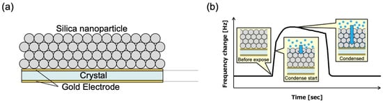
Figure 1.
Physical phenomena occurring on the sensor surface. (a) Cross-sectional conceptual diagram of sensor surface. (b) Condensation of fragrance vapor in gaps between nanoparticles.
3. Materials and Methods
3.1. Sensor Fabrication
Silica nanoparticle thin films were used as gas-capturing layers. The fabrication process of the QCM sensor modified with silica nanoparticle thin films was as follows. A non-porous silica nanoparticle dispersion solution (Sicastar, particle diameter: 50 nm, particle concentration: 25 mg/mL, Micromod Partikeltechnologie GmbH, Rostock, Germany) was diluted 10-fold with ethanol as the solvent and filtered through a filter (Whatman Mini-UniPrep, Cytiva, Waltham, MA, USA; pore size: 0.45 μm) to remove aggregates. This solution was dispensed onto one side of a quartz crystal (resonant frequency: 20 MHz, quartz crystal diameter: 8 mm, TAMADEVICE Co., Ltd., Kawasaki, Japan) at 20 μL and spin-coated at 1000 rpm for 2 min. The samples were then dried on a hot plate at 50 °C. The particle size of 50 nm was selected based on previous work by Kano et al. [18], who investigated capillary condensation behavior in non-sintered silica nanoparticle films of different particle diameters. Their study showed that films prepared from 10 nm particles exhibited slower adsorption and desorption due to finer pore radii, whereas 50 nm particles provided a more balanced response and recovery behavior. In view of these findings, the 50 nm silica nanoparticles were chosen in this study as a suitable size to achieve stable and rapid vapor responses in the QCM measurements. Figure 2b shows the SEM image of a spin-coated nanoparticle film, which was obtained by the authors using a scanning electron microscope (S-4800, Hitachi High-Tech, Tokyo, Japan). The film was spin-coated on a gold-sputtered silicon substrate using the same spin-coating conditions as those used for the QCM sensor fabrication, and is therefore representative of the coating morphology on the sensor surface.
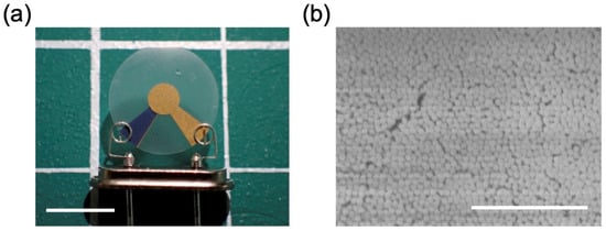
Figure 2.
QCM sensor modified with silica nanoparticle thin film on the surface. (a) Overall view of sensor elements. Scale bar = 5 mm. (b) Electron microscopy image of the silica nanoparticle thin film. Scale bar = 1 μm.
3.2. Measurement System
The headspace vapor was measured by inserting the fabricated QCM sensor into a vial containing the sample (Figure 3a). The fabricated QCM sensor was connected to a control PC using a simple portable QCM measuring device (THQ-100P-SW type, TAMADEVICE Co., Ltd., Japan). A glass vial (No. 7, capacity: 50 mL, Maruem Corporation, Osaka, Japan) was filled with 200 μL of the fragrance. This amount was determined as the minimum volume sufficient to saturate the vial headspace while maintaining a stable vapor concentration; smaller volumes resulted in unstable responses. The sensor was then fixed to a stand. To suppress the influence of the surrounding airflow, the entire setup was installed inside a draft chamber that was shut down. The sampling interval was set to 1 s. Operations such as starting/stopping measurements and setting the sampling interval were performed using the QCMeasure software (version 1.11, TAMADEVICE Co., Ltd., Japan). The measurement results were output as data for the number of samples (time), frequency, and frequency change value from the start of the measurement. To explain the changes in the time-response waveform due to differences in the vapor pressure of the fragrance, a typical response image is shown in Figure 3b.
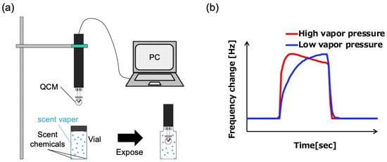
Figure 3.
(a) Schematic of the experimental system. (b) Schematic of the difference in response due to differences in apparent vapor pressure.
3.3. Measurement Procedure
The fragrance vapor was measured according to the following procedure (Figure 4). First, 200 μL of fragrance was sealed in a vial and left to stand for 5 min. Next, the sensor was placed in a vial and exposed for 5 min to allow the sensor surface to acclimate to the fragrance vapor prior to the measurement. The sensor was then removed and left to stand in the air for 5 min. Next, for the measurement, the sensor was placed in a vial and exposed to fragrance vapor. Because the time required to reach the maximum change varies depending on the fragrance, the exposure time was adjusted accordingly (specifically, preliminary measurements were conducted, and based on the results, the exposure time was set to 30, 60, or 90 s). After the measurement, the sensor was removed and left to rest in the air for 5 min. This measurement and the air resting process were repeated 12 times. The exposure time was set to 30 s for high-volatility compounds (e.g., limonene, α-terpinene, isobutyl isobutyrate, isoamyl butyrate, ethyl hexanoate, p-cymene, benzaldehyde, hexyl acetate, hexyl alcohol, benzyl acetate), 60 s for medium-volatility compounds (e.g., linalyl acetate, ethyl benzoate, undecanal), and 90 s for low-volatility compounds (e.g., phenethyl alcohol).
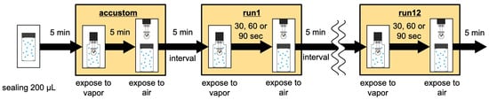
Figure 4.
Measurement procedure. Twelve consecutive measurements were taken for each fragrance.
3.4. Analysis
In this study, three characteristic quantities representing the response characteristics of each fragrance were defined from the time-response waveforms of the sensor. Specifically, these are the sensor response time t90, which represents the vapor adsorption process; the sensor recovery time t10, which represents the desorption process of condensed vapor; and Δ, where represents the slope of the response overshoot. These features were calculated based on the representative points on the response waveform (Figure 5). Accordingly, a is the initial value at the start of the exposure, b is the peak value, c is the value at the end of the exposure, and d is the frequency change value when the response decreases and stabilizes. In addition, e represents the point where the frequency change value reaches 90% of the adsorption process between A and B (e = 0.9(b − a)), and f represents the point where the frequency change value decreases to 10% of the desorption process between C and D (f = 0.1(d − c)). Each feature was calculated as follows: t90 = te − ta (time until 90% of the value increased), t10 = tf − tc (time until 90% of the value decreased), and Δ = (b − c)/(tb − tc) (slope of the graph after the peak).
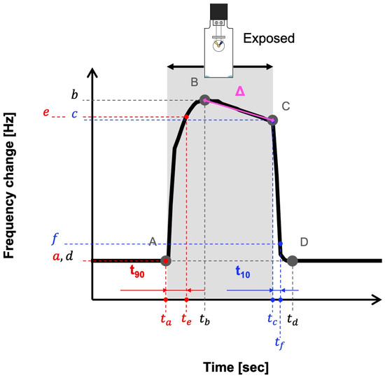
Figure 5.
Representative data and parameters representing the features. Δ: Slope after peak, t90: response time, t10: recovery time.
To investigate whether the relationship between the features obtained in this study and the vapor pressure can be applied to estimate the vapor pressure of unknown samples, cross-validation was performed. Leave-one-group-out cross-validation (LOGO-CV) was used for cross-validation. LOGO-CV divides data into groups and performs verification, which prevents information leakage within the same group [22]. In this study, each fragrance was defined as one group, and the generalization performance of the regression model using the least squares method (LSM) was evaluated using this method. Using LOGO-CV, it is possible to ensure that the same fragrance data is not duplicated in the test and training data. The implementation environment consisted of Python (v3.13.1), scikit-learn (v1.6.0), numpy (v2.2.0), and pandas (v2.2.3).
The evaluation metrics used were the root mean square error (RMSE) and mean absolute percentage error (MAPE). These metrics are widely used to evaluate the accuracy of prediction models and are considered particularly effective when dealing with data of different scales [23]. The RMSE and MAPE are defined as follows:
where N: Number of test data, : Reference value of the target quantity of the i-th test data, yi: Predicted value of the target quantity of the i-th test data. The scores were calculated for each combination of the test and training data, and the average values were used as the final scores. The predicted values were calculated using the regression equations obtained by regression analysis for each fragrance (Table S1). Statistical analysis was performed by calculating the mean and standard deviation from 12 repeated measurements for each fragrance. RMSE and MAPE were used as quantitative indicators of prediction accuracy.
The detailed analysis procedure is as follows. For each type of fragrance, 12 sets of measurement data were collected, and data that were clearly abnormal owing to operational errors were excluded. Nine sets of data were randomly selected. To ensure reproducibility, the random number generator was fixed to “random_state = 0.” The selected data were divided into 14 groups (14 types of fragrances were used) according to the fragrance type. Each group was used as test data one at a time, and the remaining data were used as training data to create 14 combinations. A model was constructed using the training data, and the predicted values y were calculated for the test data. The constructed model follows the regression equations (Equations (4)–(10)) below, depending on the number of features used. For one feature:
For two features:
For three features:
Here, each symbol is defined as follows: x1: Feature 1 (log10|Δ|), x2: Feature 2 (log10t90), x3: Feature 3 (log10t10), yn: Predicted value (n indicates the number of features used), β0: intercept, βn: regression coefficient corresponding to feature xn (n = 1, 2, 3). The subscript (xi, xj) indicates the combination of features used in the model construction (e.g., (x1, x2), (x1, x3), (x2, x3), etc.). This procedure was repeated such that all data groups were used as the test data. The RMSE was calculated for each fragrance, and the mean RMSE was calculated by dividing the total RMSE of all fragrances by the number of fragrances 14 for each combination of features. The combinations of features were set to the following seven combinations, each containing at least one of the three features (log10|Δ|, log10t90, and log10t10). (a) log10|Δ|, (b) log10t90, (c) log10t10, (d) log10|Δ|, log10t90, (e) log10|Δ|, log10t10, (f) log10t90, log10t10, (g) log10|Δ|, log10t90, log10t10. In addition, for comparison with existing methods, MAPE was calculated for the combination with the best RMSE score. Note that the data used in this analysis refer specifically to the features extracted from the measurement data (described in Section 4.3).
3.5. Fragrances
Fourteen commercially available fragrances were used in the study (Table 1). The selected fragrances cover a wide range of volatility and polarity, enabling evaluation of both polar and nonpolar compounds with different molecular weights. Because the sensing principle relies on capillary condensation and interfacial adsorption on a silica nanoparticle surface, the developed device is expected to recognize moderately volatile compounds more effectively than extremely low-volatility substances. Benzaldehyde was purchased from FUJIFILM Wako Pure Chemical Corporation (Osaka, Japan), undecanal from Tokyo Chemical Industry (Tokyo, Japan), and the others from Sigma-Aldrich (St. Louis, MO, USA). In selecting the fragrances, those that did not cause olfactory discomfort were selected to facilitate the experiment. Additionally, to calculate the vapor pressure at any temperature during the measurement, the following equation, which approximates the Clausius–Clapeyron equation, was used:
where ΔvapHm is the molar evaporation enthalpy, R is the gas constant, P0 is the standard pressure, T0 is the boiling point at standard pressure, T is an arbitrary temperature, and Pvap is the saturated vapor pressure at T. Under the following conditions, the temperature must be sufficiently below the critical temperature, the saturated vapor pressure must be sufficiently low, and the temperature difference from the boiling point must be small. This allowed the volume change due to evaporation to be approximated as the volume change of vapor and the volume of vapor to be approximated as the volume of an ideal gas. The temperature and pressure dependences of the molar evaporation enthalpy were ignored. In this study, the temperature was measured at 5-min intervals during 12 consecutive measurements for each sample, and the vapor pressure was calculated based on the average temperature.

Table 1.
Fragrances used in the measurements. The reference vapor pressure at the measurement temperature was corrected using the molar vaporization enthalpy and boiling point values from the literature. The molar enthalpy of vaporization and boiling point at standard pressure were obtained from the NIST Chemistry WebBook (Standard Reference Data, SRD 69) and ChemSpider (Royal Society of Chemistry).
The vapor pressure values at the measurement temperature were calculated from the Clausius–Clapeyron equation using the literature data of boiling point and enthalpy of vaporization, and are referred to as the reference vapor pressure in this study. The term apparent vapor pressure is used hereafter to indicate the vapor pressure values predicted from the QCM response data using the regression model described in Section 4.4.
4. Results and Discussions
4.1. Sensor Responsiveness
To determine whether each fragrance exhibited unique responsiveness, we plotted time-dependent changes in the frequency change values for each fragrance (Figure 6). The frequency change values were normalized by dividing them by the maximum frequency change value. This normalized frequency change value is referred to as Δfnorm. Depending on the fragrance, the behavior of Δfnorm increased from 0 to its maximum value, and the slope (rate of decrease) after the peak differed. These results indicate that there are differences in the evaporation speed from the pores of the nanoparticle thin film and the condensation speed in the pores, depending on the fragrance. Thus, it was confirmed that this sensor can obtain different responses depending on the fragrance.
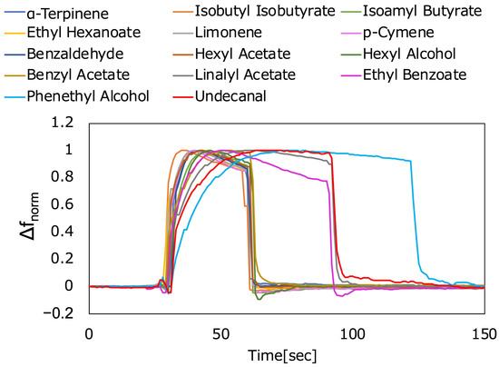
Figure 6.
Response for each fragrance. Δfnorm represents the normalized frequency change value.
4.2. Measurement Reproducibility
To investigate the reproducibility of the sensor, more than 10 consecutive measurements were performed for each fragrance. The vertical axis was normalized in the same manner, as shown in Figure 6. For example, the plots for limonene showed good agreement (Figure 7). Similarly, the plots for all fragrances used showed good agreement (Figure S1). These results confirm that the sensor responded reproducibly to the fragrances used. All consecutive measurements were performed within two hours. During the measurements, the temperature and humidity did not change significantly, and the measurements were stable. These results suggest that the proposed measurement system can be used to stably measure fragrances with good reproducibility in typical indoor environments. Additional response data for all fragrances are provided in the Supplementary Materials (Figures S1–S4).
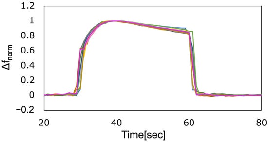
Figure 7.
Response to limonene, which was measured consecutively (N = 12).
4.3. Relationship Between Sensor Response and Vapor Pressure
By extracting the characteristic quantities from the obtained responses, we investigated the relationship between the sensor response and vapor pressure. In a previous study [17], parameters such as the adsorption process, desorption process, slope between the adsorption and desorption processes, and maximum response value were extracted, and kernel ridge regression was used to predict the alcohol content of the unknown alcohol. In this study, we applied the same approach and plotted the relationship between the three features ∆, t90, and t10, and the reference vapor pressure Pvap using common logarithms (Figure 8). Because the slope is negative, we applied common logarithms to the absolute values. All three parameters showed a linear correlation with the vapor pressure. The larger log10|Δ|, the higher log10Pvap, and the larger log10t90 and log10t10, the lower log10Pvap. This reflects that, as the vapor pressure of the fragrance increases, condensation and evaporation in the pores of the nanoparticle thin film occur more rapidly, whereas in substances with lower vapor pressure, these processes occur more slowly. These results suggest that it may be possible to estimate the vapor pressure by comprehensively interpreting multiple parameters based on differences in the adsorption and desorption rates of fragrances obtained using this sensor within the vapor pressure range of 1–490 Pa. These findings suggest that the nanostructured silica surface influences the adsorption–desorption rate balance of fragrance molecules, thereby affecting the apparent vapor pressure estimated from the QCM responses.
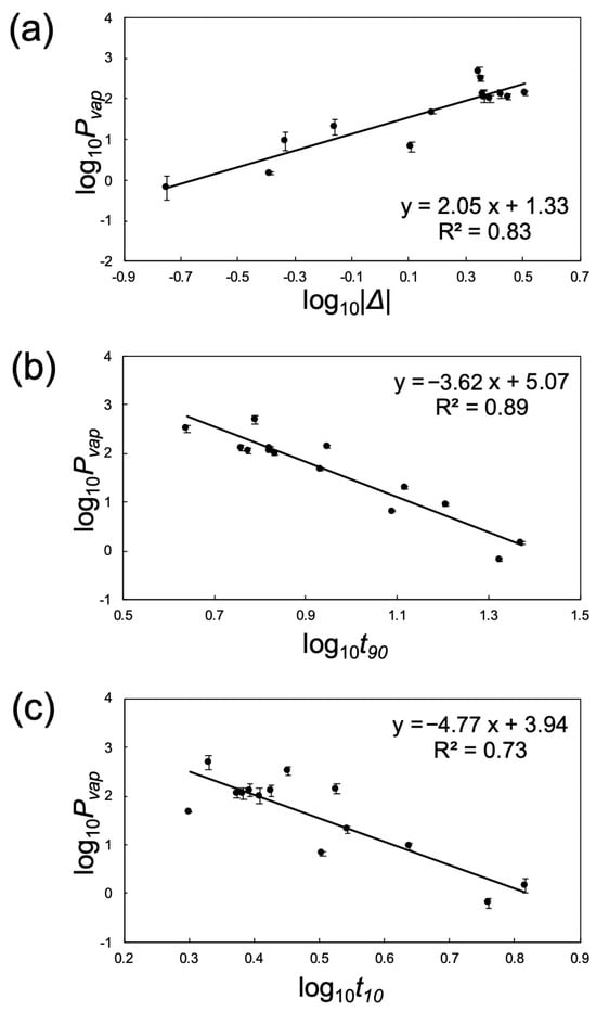
Figure 8.
Relationship between apparent vapor pressure Pvap and features Δ (a), t90 (b), and t10 (c).
While low vapor pressure generally slows desorption, the prediction error is not governed by vapor pressure alone. Compound-specific interfacial effects—such as molecular polarity, hydrogen-bonding ability to surface silanols, and surface tension that affects capillary condensation—also modulate the adsorption and desorption dynamics on the silica nanoparticle surface. These effects can shift the feature triplet (Δ, t90, t10) relative to the regression trend and thus influence the estimation accuracy.
The parameters Δ, t90, and t10 correspond to the apparent adsorption and desorption rates; specifically, t90 and t10 quantitatively represent the characteristic times of adsorption and desorption, respectively.
4.4. Cross-Validation
In this study, the apparent vapor pressure denotes the vapor pressure predicted from the QCM response features, whereas the reference vapor pressure refers to the literature-based values calculated from thermodynamic data. The regression model was trained to reproduce the reference vapor pressure using the apparent vapor pressure derived from QCM responses.
To investigate the applicability of this method for estimating the vapor pressure of unknown samples, a cross-validation was performed. LOGO-CV was used to evaluate regression models (Table 2). The prediction model was built based on the apparent vapor pressure values. First, when comparing cases with a single feature (Table 2 (a), (b), (c)), the RMSE was smallest for log10t90, followed by log10|Δ|, and log10t10 in descending order. This indicated that the model using log10t90 demonstrated the highest prediction accuracy. Similarly, in Figure 8, the R2 value was the highest for log10t90, followed by log10|Δ| and log10t10, indicating that the model using log10t90 showed the highest correlation. These results were consistent. Next, when comparing the cases with two features (Table 2 (d), (e), (f)), the RMSE was smallest for “log10|Δ|, log10t90,” followed by “log10t90, log10t10,” and “log10|Δ|, log10t10.” In all two-variable models, the RMSE was smaller than that of the single-feature regression model, indicating an improvement in error. Furthermore, the regression model using all three features (log10|Δ|, log10t90, and log10t10) (Table 2 (g)) showed a smaller RMSE than any of the single- and two-variable models. This suggests that combining multiple features contributes to improving the prediction accuracy. Next, the MAPE of the predicted values relative to reference vapor pressure values was calculated for the three-variable model that showed the highest prediction accuracy (Table 3). The MAPE was smallest for phenethyl alcohol (19.3%) and largest for ethyl benzoate (279%).
Table 2.
Mean RMSE for each combination of features.
Table 3.
Mean Absolute Percentage Error (MAPE) for each fragrance.
Notably, phenethyl alcohol, which has a similarly low vapor pressure (1.44 Pa) but stronger polarity and hydrogen-bonding ability, exhibited a small MAPE, whereas undecanal and ethyl benzoate, which are less polar, showed larger deviations. This suggests that interfacial interactions, in addition to vapor pressure, affect the dynamic response.
4.5. Comparison with Existing Vapor Pressure Measurement Methods
The method used in this study was compared with existing vapor pressure measurement methods, including the static method, boiling point method, isoteniscope method, gas saturation method, DSC method, and triple expansion method, in terms of accuracy, measurement time, required liquid volume, and the necessity of cleaning the apparatus. First, in terms of accuracy, the reported values for the existing methods were approximately 1% for the static method [24],3% for the boiling point method [25], 5–10% for the isoteniscope method [26], 10–30% for the gas saturation method [26], less than 1% for the DSC method [27], and approximately 2% for the triple-expansion method (e.g., MINIVAP VPL Vision (Grabner Instruments, Vienna, Austria) specifications) [28]. On the other hand, the method used in this study yielded an MAPE of 19.3–220%, indicating a lower accuracy compared to existing methods. Regarding the measurement time, in the static method, it has been reported that it took over 6 h for the pressure to reach equilibrium because of the diffusion of volatile impurities in the liquid during measurements of tetrakisethylmethylaminohafnium [29]. In the boiling point method, it is estimated that approximately 30 min to 1 h are required to heat the sample to the target temperature, approximately 15 to 30 min to confirm equilibrium, and approximately 15 to 30 min for the measurement itself. Therefore, although there is no clear indication of the required time in the literature, considering these factors, the total measurement time was estimated to be approximately 1 to 2 h. In the isoteniscope method, there are reports indicating that measurements were performed within 1 to 2 h, including heating and equilibration procedures [30]. In the gas saturation method, when measuring eicosane, there are reports of continuously flowing gas for approximately seven days [31]. In the DSC method, there are reports of approximately 2 h for a series of measurements of decane, dodecane, and tetradecane [32]. The triple expansion method takes at least approximately 5 min (e.g., according to the specifications of the MiniVap VPL Vision) [28]. However, the method used in this study requires only a few minutes for the measurement itself, significantly reducing the measurement time compared with existing methods. Regarding the required liquid volume, the static method requires approximately 0.5 mL [24], the boiling point method requires approximately 150 mL [33], the isoteniscope method requires approximately 10 mL [33], and the gas saturation method requires approximately 1 g [33]. The DSC method requires approximately 1 g [33], and the triple expansion method requires 3.2 mL, including the cleaning process (e.g., according to the specifications of the MiniVap VPL Vision) [28]. In contrast, the method used in this study can measure with 200 μL of liquid, making it highly convenient in terms of sample consumption. Regarding the necessity of cleaning after measurement, in all methods—the static method [31], boiling point method [34], isoteniscope method [35], gas saturation method [31], DSC method [36], and triple expansion method [28]—cleaning is often required because of sample residue or contamination inside the apparatus, which requires time and effort when switching between measurements. However, the method used in this study does not require cleaning before or after the measurement and allows consecutive measurements of multiple types of samples. This was expected to significantly improve the overall efficiency of the experiment.
5. Conclusions
In this study, we aimed to develop a method for quickly and easily estimating vapor pressure based on the characteristics related to vapor pressure, which is an important indicator of the volatility of fragrances. Fragrance vapors were measured using a QCM sensor modified with a thin film of silica nanoparticles. When measuring fragrances with different vapor pressures, clear differences in the sensor response waveforms (rise and fall) were observed for each fragrance, quantitatively demonstrating the influence of the vapor pressure on the sensor response. In particular, for fragrances with a high vapor pressure, condensation and evaporation occurred more rapidly in the nanoscale pores, which was reflected in the response and recovery times. A regression model using multiple features (Δ, t90, and t10) extracted from the response waveforms showed smaller prediction errors than when using a single feature, contributing to improved vapor pressure estimation accuracy. This method also demonstrated a better response for low-polarity fragrances that were difficult to measure using impedance-type sensors. This method is significant as a new, simple measurement technique because it enables nondestructive evaluation in a shorter time and with less sample volume than existing vapor pressure measurement methods for the same measurement targets. In fact, this method requires only a few minutes of measurement time, 200 µL of liquid, and no cleaning of the device, making it useful as a rapid screening method in the development of perfumes and air fresheners. The results also suggest that the nanostructured silica surface may influence the interfacial adsorption–desorption behavior of fragrance molecules, thereby affecting their apparent vapor pressure characteristics. Furthermore, by applying this method to volatile substances other than fragrances, it is expected to be applicable to a wide range of fields, such as estimating the vapor pressure of harmful substances and assessing environmental risks. This method may show reduced accuracy for highly polar or charged compounds (e.g., amines and carboxylic acids) because of strong hydrogen-bonding or electrostatic interactions with surface silanol groups, as well as for heavy molecules (>200 Da) that diffuse and desorb slowly from the nanoporous layer. Nevertheless, for most neutral organic compounds within the tested volatility range, the method provides reproducible and consistent vapor pressure estimations.
Supplementary Materials
The following supporting information can be downloaded at: https://www.mdpi.com/article/10.3390/app152111648/s1, Figures S1: Responses to continuous measurements (N = 12): (a) α-terpinene, (b) isobutyl isobutyrate, (c) isoamyl butyrate, and (d) ethylhexanoate; Figure S2: Responses to continuous measurements (N = 12): (a) p-cymene, (b) benzaldehyde, (c) hexyl acetate, and (d) hexyl alcohol; Figure S3: Responses to continuous measurements (N = 12): (a) benzylacetate (b) linalyl acetate, (c) ethyl benzoate, and (d) phenethyl alcohol; Figure S4: Responses to continuous measurements (N = 12): undecanal; Table S1: Regression equations used to calculate predicted values.
Author Contributions
Conceptualization, H.H. and S.K.; methodology, H.H. and S.K.; formal analysis, H.H. and Y.M.; investigation, H.H. and Y.M.; data curation, H.H. and Y.M.; writing—original draft preparation, H.H., Y.M. and S.K.; writing—review and editing, M.H.; visualization, H.H. and Y.M.; supervision, M.H.; project administration, H.H. All authors have read and agreed to the published version of the manuscript.
Funding
This research received no external funding.
Institutional Review Board Statement
Not applicable.
Informed Consent Statement
Not applicable.
Data Availability Statement
The original contributions presented in this study are included in the article. Further inquiries can be directed to the corresponding author.
Conflicts of Interest
The authors declare no conflicts of interest.
References
- Rodrigues, A.E.; Nogueira, I.; Faria, R.P.V. Perfume and Flavor Engineering: A Chemical Engineering Perspective. Molecules 2021, 26, 3095. [Google Scholar] [CrossRef]
- Kasting, G.B.; Saiyasombati, P. A physico-chemical properties based model for estimating evaporation and absorption rates of perfumes from skin. Int. J. Cosmet. Sci. 2001, 23, 49–58. [Google Scholar] [CrossRef]
- Schwarzenbach, R.; Bertschi, L. Models to assess perfume diffusion from skin. Int. J. Cosmet. Sci. 2001, 23, 85–98. [Google Scholar] [CrossRef]
- Almeida, R.N.; Hartz, J.G.M.; Costa, P.F.; Rodrigues, A.E.; Vargas, R.M.F.; Cassel, E. Permeability coefficients and vapour pressure determination for fragrance materials. Int. J. Cosmet. Sci. 2021, 43, 225–234. [Google Scholar] [CrossRef]
- Smith, A.; Menzies, A.W.C. Studies in vapor pressure: III. A static method for determining the vapor pressures of solids and liquids. J. Am. Chem. Soc. 1910, 32, 1412–1434. [Google Scholar] [CrossRef]
- Barton, J.L.; Bloom, H. A Boiling Point Method for Determination of Vapor Pressures of Molten Salts. J. Phys. Chem. 1956, 60, 1413–1416. [Google Scholar] [CrossRef]
- ASTM D2879-23; Standard Test Method for Vapor Pressure-Temperature Relationship and Initial Decomposition Temperature of Liquids by Isoteniscope. ASTM International: West Conshohocken, PA, USA, 2023.
- U.S. Government Publishing Office. Vapor Pressure; U.S. Government Publishing Office: Washington, DC, USA, 2024. [Google Scholar]
- TA Instruments. Boiling Point and Vapor Pressure Measurement by Pressure DSC: TA Instruments. Available online: https://www.tainstruments.com/pdf/literature/TA201.pdf (accessed on 16 June 2025).
- ASTM D6378-22; Standard Test Method for Determination of Vapor Pressure (VPX) of Petroleum Products, Hydrocarbons, and Hydrocarbon-Oxygenate Mixtures (Triple Expansion Method). ASTM International: West Conshohocken, PA, USA, 2022.
- Rianjanu, A.; Hasanah, S.A.; Nugroho, D.B.; Kusumaatmaja, A.; Roto, R.; Triyana, K. Polyvinyl Acetate Film-Based Quartz Crystal Microbalance for the Detection of Benzene, Toluene, and Xylene Vapors in Air. Chemosensors 2019, 7, 20. [Google Scholar] [CrossRef]
- Gao, N.B.; Li, H.Y.; Zhang, W.H.; Zhang, Y.Z.; Zeng, Y.; Hu, Z.X.; Liu, J.Y.; Jiang, J.J.; Miao, L.; Yi, F.; et al. QCM-based humidity sensor and sensing properties employing colloidal SnO2 nanowires. Sens. Actuators B-Chem. 2019, 293, 129–135. [Google Scholar] [CrossRef]
- Ayad, M.M.; Torad, N.L.; Minisy, I.M.; Izriq, R.; Ebeid, E.M. A wide range sensor of a 3D mesoporous silica coated QCM electrodes for the detection of volatile organic compounds. J. Porous Mat. 2019, 26, 1731–1741. [Google Scholar] [CrossRef]
- Rianjanu, A.; Triyana, K.; Nugroho, D.B.; Kusumaatmaja, A.; Roto, R. Electrospun polyvinyl acetate nanofiber modified quartz crystal microbalance for detection of primary alcohol vapor. Sens. Actuator A-Phys. 2020, 301, 111742. [Google Scholar] [CrossRef]
- Wang, X.H.; Zhang, J.; Zhu, Z.Q. Ammonia sensing characteristics of ZnO nanowires studied by quartz crystal microbalance. Appl. Surf. Sci. 2006, 252, 2404–2411. [Google Scholar] [CrossRef]
- Quang, V.V.; Hung, V.N.; Tuan, L.A.; Phan, V.N.; Huy, T.Q.; Quy, N.V. Graphene-coated quartz crystal microbalance for detection of volatile organic compounds at room temperature. Thin Solid Films 2014, 568, 6–12. [Google Scholar] [CrossRef]
- Shiba, K.; Tamura, R.; Imamura, G.; Yoshikawa, G. Data-driven nanomechanical sensing: Specific information extraction from a complex system. Sci. Rep. 2017, 7, 3661. [Google Scholar] [CrossRef]
- Kano, S.; Mekaru, H. Liquid-dependent impedance induced by vapor condensation and percolation in nanoparticle film. Nanotechnology 2022, 33, 105702. [Google Scholar] [CrossRef]
- Röck, F.; Barsan, N.; Weimar, U. Electronic nose:: Current status and future trends. Chem. Rev. 2008, 108, 705–725. [Google Scholar] [CrossRef]
- Brunauer, S.; Emmett, P.H.; Teller, E. Adsorption of gases in multimolecular layers. J. Am. Chem. Soc. 1938, 60, 309–319. [Google Scholar] [CrossRef]
- Sauerbrey, G. Verwendung Von Schwingquarzen Zur Wagung Dunner Schichten Und Zur Mikrowagung. Z. Für Phys. 1959, 155, 206–222. [Google Scholar] [CrossRef]
- Pedregosa, F.; Varoquaux, G.; Gramfort, A.; Michel, V.; Thirion, B.; Grisel, O.; Blondel, M.; Prettenhofer, P.; Weiss, R.; Dubourg, V.; et al. Scikit-learn: Machine Learning in Python. J. Mach. Learn. Res. 2011, 12, 2825–2830. [Google Scholar]
- Hyndman, R.J.; Koehler, A.B. Another look at measures of forecast accuracy. Int. J. Forecast. 2006, 22, 679–688. [Google Scholar] [CrossRef]
- Bhagwat, R.; Sanadhya, S.; Gulotty, E.; Tucker, Z.; Ashfeld, B.; Moghaddam, S. High-precision vapor pressure measurement apparatus with facile and inexpensive construction. Meas. Sci. Technol. 2022, 33, 067002. [Google Scholar] [CrossRef]
- Ambrose, D.; Ewing, M.B.; Ghiassee, N.B.; Ochoa, J.C.S. The Ebulliometric Method of Vapor-Pressure Measurement—Vapor-Pressures of Benzene, Hexafluorobenzene, and Naphthalene. J. Chem. Thermodyn. 1990, 22, 589–605. [Google Scholar] [CrossRef]
- U.S. Environmental Protection Agency. Product Properties Test Guidelines OPPTS 830.7950: Vapor Pressure; Contract No.: EPA 712–C–96–043; U.S. Environmental Protection Agency: Washington, DC, USA, 1996. [Google Scholar]
- deBarros, T.M.V.R.; Santos, R.C.; Fernandes, A.C.; daPiedade, M.E.M. Accuracy and precision of heat capacity measurements using a heat flux differential scanning calorimeter. Thermochim. Acta 1995, 269, 51–60. [Google Scholar] [CrossRef]
- Grabner Instruments. Absolute Vapor Pressure of Paints, Varnishes, Solvents; Application Note; Grabner Instruments: Vienna, Austria; Available online: https://www.grabner-instruments.com (accessed on 29 October 2025).
- Berg, R.F. Correcting “Static” Measurements of Vapor Pressure for Time Dependence Due to Diffusion and Decomposition. J. Chem. Eng. Data 2015, 60, 3496–3505. [Google Scholar] [CrossRef]
- OECD. OECD Guidelines for the Testing of Chemicals, Test No. 104: Vapour Pressure; Contract No.: OECD TG 104; Organisation for Economic Co-operation and Development: Paris, France, 2006. [Google Scholar]
- Widegren, J.A.; Harvey, A.H.; McLinden, M.O.; Bruno, T.J. Vapor Pressure Measurements by the Gas Saturation Method: The Influence of the Carrier Gas. J. Chem. Eng. Data 2015, 60, 1173–1180. [Google Scholar] [CrossRef]
- Casserino, M.; Blevins, D.R.; Sanders, R.N. An improved method for measuring vapor pressure by DSC with automated pressure control. Thermochim. Acta 1996, 284, 145–152. [Google Scholar] [CrossRef]
- Toray Research Center. Vapor Pressure: Toray Research Center. Available online: https://www.toray-research.co.jp/en/technical-info/analysis/Vapor_Pressure_measurement.html (accessed on 30 May 2025).
- ASTM E1719-05; Standard Test Method for Vapor Pressure of Liquids by Ebulliometry. ASTM International: West Conshohocken, PA, USA, 2012.
- ASTM D2879-97; Standard Test Method for Vapor Pressure-Temperature Relationship and Initial Decomposition Temperature of Liquids by Isoteniscope. ASTM International: West Conshohocken, PA, USA, 1997.
- PerkinElmer. Determining Vapor Pressure by Pressure DSC; Contract No.: Application Note 010056_01; PerkinElmer: Norwalk, CT, USA, 2004. [Google Scholar]
Disclaimer/Publisher’s Note: The statements, opinions and data contained in all publications are solely those of the individual author(s) and contributor(s) and not of MDPI and/or the editor(s). MDPI and/or the editor(s) disclaim responsibility for any injury to people or property resulting from any ideas, methods, instructions or products referred to in the content. |
© 2025 by the authors. Licensee MDPI, Basel, Switzerland. This article is an open access article distributed under the terms and conditions of the Creative Commons Attribution (CC BY) license (https://creativecommons.org/licenses/by/4.0/).