Abstract
At present, the research on the microclimate of urban parks mainly focuses on the univariate or multivariate research contents of park design elements, and there are few analyses that can combine the park with the surrounding regional environment to jointly explore the cooling mechanism of park design elements. This study takes the People’s Park in Urumqi, a typical oasis city in an arid area, as the research object. Combined with different land use natures (park area/residential area), it analyzes the spatiotemporal variation law of temperature through mobile meteorological monitoring in different periods of summer and autumn and optimizes the buffer zone to further compare the performance of the multiple linear regression model and three machine learning models. The selection of the optimal model for collaborative analysis and comparison revealed the dominant variables and their threshold effects affecting the temperature of the park area and the residential area. The results show that: (1) In multi-scenario comparisons, a larger buffer has a better fitting effect. (2) The random forest model is the best model for temperature prediction in the study area. (3) The dominant factors of temperature in different seasons show significant differences, and only a few periods have cross-seasonal persistence. In the park area, the green coverage rate and road network density play a leading and influential role, while in the residential area, the influence of water cover ratio is more obvious. Furthermore, the influence direction of residential area indicators on temperature shows opposite trends in the morning and afternoon periods. (4) There are obvious limited-threshold effects on the influence of dominant factors on temperature in different regions. It is suggested that in the urban spatial layout, while considering the differences for different utilization Spaces, collaborative planning should be carried out. These findings offer new insights into temperature drivers and provide practical references for urban planners.
1. Introduction
With accelerated global urbanization, urban ecosystems are facing unprecedented structural changes. Over half of the global population currently resides in cities, a figure projected to reach 70% by 2050 [1]. Artificially increasing urban radiant heat leads to significant changes in underlying surface characteristics and energy balance [2], which alter the urban climate and even produce the heat island effect (UHI). This problem is particularly severe in hot and arid regions, where climatic conditions such as high temperatures and intense solar radiation will exacerbate the risks. Heat exposure also puts pressure on the mental and physical well-being of the public [3,4]. Urban parks have been proven to mitigate the UHI effect through shading and evapotranspiration [5,6]. The current research mainly focuses on the spatial extent and spatiotemporal dynamics of park cooling at a macro level [7,8], generally observing lower temperatures around parks compared to warmer urban centers. At a microscale, factors such as green coverage rate (GCR), impervious surface percentage (ISP), and water cover ratio (WCR) within parks are recognized as key influencers on cooling intensity [9]. Despite multi-faceted explorations, the generalizability of findings remains constrained by inconsistencies in data acquisition methods.
Land surface temperature is commonly acquired via three approaches: remote sensing inversion, which offers broad coverage but may lack accuracy or temporal resolution [10]; fixed weather stations, which provide reliable time-series data but have limited spatial representation [11]; and numerical modeling, which simulates atmospheric processes but is often hampered by parametric uncertainties. Recently, mobile monitoring—using vehicle-mounted or wearable sensors—has gained traction for its ability to capture high-resolution, spatially continuous microclimatic data, offering distinct advantages for microscale analysis. The emergence of such high-resolution data calls for analytical methods capable of leveraging detailed spatiotemporal information.
To exploit this potential for deeper insight, researchers have employed a range of analytical techniques to assess cooling effects. It is relatively common to reveal the cooling effect through buffer zone analysis and statistical analysis method [12]. The regression model in traditional analysis methods has certain limitations [13]. For example, multiple linear regression (MLR) is often applied due to its efficiency and simplicity [14], but it is difficult to capture nonlinear relationships and variable interactions [15]. Machine learning (ML) can provide flexible model structures and efficient algorithms to capture nonlinear relationships. For instance, random forests (RF), extreme gradient boosting (XGBoost), and light gradient boosters (LightGBM) have been extensively adopted to achieve high-precision simulation and prediction of the spatial differentiation of near-surface temperatures. For instance, Komeh, Z. [16] and Tanoori, G. et al. [17] utilized XGBoost and convolutional neural networks to automatically extract urban morphological features from high-resolution remote sensing images, significantly improving the simulation accuracy of the spatial pattern of UHI intensity. Such findings generally confirm that GCR and the ISP are the two most influential dominant factors in explaining the spatial heterogeneity of the urban thermal environment. In studies targeting the cooling effects of blue-green infrastructure such as parks and water bodies, some scholars have successfully quantified the cooling amplitude and effective influence range of different landscape types [18,19]. Furthermore, some cutting-edge research has begun to integrate small-scale meteorological data with detailed urban morphology parameters. By leveraging machine learning models, these methods can rapidly simulate wind fields within small areas or predict thermal comfort indices [20,21], providing efficient analytical tools for comprehensive urban thermal environment assessment. Although significant progress has been made in research, the existing study areas are mostly cities in temperate (humid or semi-humid), tropical, subtropical, Mediterranean and cold climate regions.
In summary, the current achievements still have obvious limitations: they mainly rely on macro-scale data models and lack micro-scale movement monitoring, making it difficult to precisely identify small-scale thermal environment changes; the research areas are mostly concentrated in humid and mid-latitude climate zones, and case studies from arid regions are scarce; they mostly focus on influencing factors within a single season and lack comparisons between inside and outside the park as well as multi-season analysis; moreover, the existing models have insufficient stability at different temporal and spatial scales, and their applicability in arid regions needs further verification. Based on this context, this study attempts to contribute to the understanding of microclimate modeling in arid regions by taking Urumqi, a typical arid oasis city, as a case study. We utilize mobile monitoring data from People’s Park and adjacent residential areas across different periods in summer and autumn for a comparative analysis. The objectives of this work are: The purpose of this paper is (1) To characterize the spatiotemporal temperature distribution in and around urban parks using high-resolution mobile monitoring data collected in both summer and autumn; (2) quantify the cooling extent of parks by establishing multi-range buffers (10–100 m) and identify the optimal effective distance for modeling; (3) employ interpretable machine learning to uncover the dominant factors and nonlinear threshold effects that differentiate intra-park and extra-park thermal environments. The findings are expected to provide insights into context-specific climatic regulation strategies and support collaborative urban planning in arid cities.
2. Materials and Methods
2.1. Study Area
Urumqi (86°37′33″–88°58′24″ E, 42°45′32″–44°08′00″ N) is located in the hinterland of the Eurasian continent, located in the transition zone between the alluvial fan at the northern foot of the Tianshan Mountains and the southern margin of the Junger Basin, and is the central city of the core area of the Silk Road Economic Belt. The climate of the city is a typical temperate continental arid climate, with dry summers and cold, extended winters. During the peak summer months of July and August, the average temperature reaches 25 °C, with extreme heat occasionally pushing temperatures above 40 °C. In contrast, winters are notably chilly, with the average temperature in January, the coldest month, dropping to −15 °C, and minimum temperatures sometimes falling below −25 °C. As the largest city in Central Asia within 1500 km (built-up area of 545.10 km2), it has a permanent population of 4,084,800 in 2023, a population density of 7492 people/km2, and an urbanization rate of 96.56%, ranking first in Northwest China. Urumqi’s high urbanization rate and limited built-up area make urban planning and layout particularly important. In this study, new urban parks and urban parks with large undulating terrain were excluded to ensure the accuracy and reliability of the results, as the difference in altitude may lead to inaccuracies in the data. The park covers an area of 300,000 square meters, with a rectangular layout as a whole, about 1000 m long from north to south, and an average width of 250 m from east to west, and the terrain in the area is extremely flat, so the temperature difference caused by topographic factors can be ignored. With a green area of 240,000 square meters, a lake area of 18,000 square meters, and a GCR of 96%, the park is the largest and oldest comprehensive park in the center of Urumqi City, integrating culture, recreation, leisure, fitness, and other functions. To further explore the cooling effect of the park and collect as much meteorological data as possible, and to ensure that the monitoring route can adequately cover most areas of the park and residential areas in terms of data collection, we designed a mobile monitoring route and, at the same time, selected an area, where there are fewer buildings, good air circulation, and where the air temperature is weakly affected by the surrounding environment, for fixed-point detection (Figure 1).
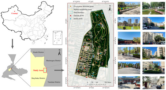
Figure 1.
Locations of study areas and mobile monitoring lines.
2.2. Experimental Design and Data Collection
The Kestrel instrument is designed, manufactured, sold, and supported by Nielsen Kellerman in Boothwyn, PA, USA. The Kestrel 5400 model mainly monitors meteorological data such as temperature, humidity, and wind speed. Monitoring was carried out using the Kestrel 5500 handheld weather recorder from the same manufacturer. The Garmin Etrex 201, developed and manufactured by Garmin International Avionics Co., Ltd., in Olathe, KS, USA, is used to monitor routes and latitude and longitude on the move and served as the GPS unit. All of the movement measures in this survey were captured by researchers who walked at a steady pace along a predetermined path with handheld monitors. Each person holds a basket of equipment with an action camera, automatic temperature recording instruments, a mobile weather station, and a GPS. We adopted a fixed monitoring route to collect the measurement values and walked the same path at all monitoring times. The monitoring of average walking speed is conducted at 4.4 km/h, with the instrument placed at a height aligned with the breathing zone, ranging from 1.2 to 1.5 m [22]. The route was designed to comprehensively and systematically cover a variety of microenvironments, including sun-exposed open areas (e.g., plazas, unshaded roads), partially shaded transition zones, fully shaded areas, core green spaces, water edges, and surrounding residential streets, ensuring broad spatial representation of the study area. Regarding the spatial distribution of the observed values, the data points are not randomly scattered or concentrated in a few locations but are essentially uniformly distributed along the predefined 10.5 km walking route. This spatial coverage was achieved by maintaining a constant walking speed (4.4 km/h) combined with periodic data logging at 5 s intervals. This setup was designed to ensure synchronized, continuous, and high-density sampling of the thermal environment across the study area (the park and surrounding residential zones). The specific route is illustrated in Figure 1. Before the experiment, all instruments are calibrated and verified under uniform conditions. Meanwhile, street view videos, temperature, humidity, and GPS tracking data are collected from fixed reference points for reference and analysis of background temperature. The device is preheated for 10 min and synchronized to the same time setting. Details regarding the kinds of equipment and configurations utilized in the study can be found in Table 1.

Table 1.
Monitors instrument parameters.
According to existing literature, representative periods within a season are often selected for micro-scale movement monitoring [8,23]. Urumqi experiences a temperate continental climate, with summers (June–August) being hot, dry, and stable. This study selected four consecutive sunny and cloudless days in mid-July to monitor local microclimate characteristics in summer. Similarly, the autumn (September–November) was monitored over three consecutive sunny and cloudless days in mid-October. Such weather conditions have the most significant impact on human thermal behavior and represent typical scenarios of key concern in urban planning. Monitoring commenced at 08:30 and 15:00, with the total distance of the monitoring route being 10.54 km and the entire journey lasting approximately 2.5 h. The timing of monitoring is affected by the pedestrian flow in the park. These two periods capture the thermodynamic competition between active anthropogenic heat sources and natural cooling regulation, respectively. After 08:30, the rush hour of commuting leads to the generation of exhaust emissions and frictional heat from roads. Coupled with the metabolic heat from the human body generated by the dense flow of people in the park in the early morning and the residual heat released by the start-up of building air conditioners, as well as the intensification of solar radiation, it intensifies the differences in heat absorption by surface materials. After 15:00, the number of tourists and traffic gradually decreases. The heat stored in the roads and buildings continues to be released, and the evapotranspiration of the shaded vegetation reaches its peak. The focus of this study is to obtain temperature data, thereby investigating the spatiotemporal variation characteristics of temperature and its influencing factors in urban parks and adjacent residential areas. This influence is most obvious on days with clearer skies and more stable weather conditions. Therefore, it is logical to choose such a data collection date within the measurement cycle [24] (Table 2).
Table 2.
Meteorological data for monitoring day.
Because the temperature changes continuously with time during the monitoring period, to remove the influence of time on the data [25,26],. Reference has been made to the existing literature using the Optimized Noise Abatement Algorithm developed by the U.S. Environmental Protection Agency to calibrate the mobile measurements to reduce the errors in the mobile monitoring data as shown in Equations (1) and (2).
This calibration method effectively eliminates the influence of temperature temporal variations on the mobile monitoring data, ensuring the spatial comparability of temperature data from different locations. Figure 2 illustrates the overall framework of this study.
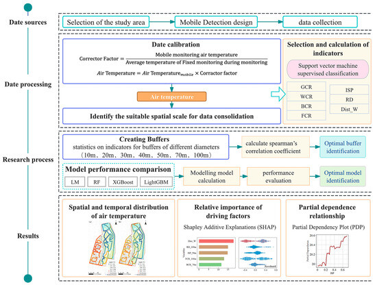
Figure 2.
Study framework.
2.3. Selection and Calculation of Indicators
In order to better analyses the influencing factors of the temperature in the study area, this study selected a total of 7 influential indicators the different characteristics of the two areas. The land use nature of parks is different from that of residential areas. One is mainly green space, and the other is mainly buildings. Therefore, the selected indicators should reflect their respective characteristics. The influencing factors of the park include GCR, WCR, ISP, Road Density (RD), and distance to waterbody (Dist_W). The influencing factors of residential areas include building coverage ratio (BCR), floor area ratio (FCR), ISP, RD, and Dist_W. BCR and FCR reflect the intensity of three-dimensional development, heat radiation exchange, and ventilation efficiency. ISP, GCR, and WCR exhibit the characteristics of natural surface thermal balance, corresponding to the effects of surface hardening heat storage, vegetation transpiration cooling, and water evaporation. The RD quantifies the intensity of traffic heat sources and reflects exhaust emissions and anthropogenic thermal disturbances, while the Dist_W directly characterizes the potential for gradient diffusion of natural cooling sources. These indicators jointly determine the enhancement or weakening of the regional cooling effect through the dynamic game among hardening expansion, cold source configuration, and spatial organization (Table 3). While fundamental variables such as albedo, vegetation canopy density, and direct anthropogenic heat flux are theoretically important in microclimate studies, they are challenging to quantify accurately at the neighborhood scale. Therefore, this study employed a series of practical and effective proxy indicators—such as ISP, GCR, and RD—that balance theoretical relevance with measurable reality. The coverage of ISP indirectly reflects the difference between surface albedo and heat storage capacity; the GCR macroscopically represents the cooling efficiency of vegetation; and the RD serves as a reliable indicator of anthropogenic heat emissions related to transportation. The selection of these indicators is based on three fundamental principles: Firstly, they are both rooted in theory and have significance in urban planning practice. Secondly, they are easy to understand and calculate; finally, they have almost no redundancy [27].
Table 3.
Definition and calculation formula of urban morphology indicators.
2.4. Identify the Suitable Spatial Scale for Data Consolidation
Due to the short time interval and large data volume of the mobile temperature monitoring data in this study, determining the spatial scale of data aggregation is crucial for reducing uncertainties in geographic analysis [28]. In order to maintain the spatial variance of the temperature distribution, we modeled the dataset using the empirical semi-variance function in geostatistics to determine the optimal spatial aggregation scale [29]. The results of the semi-variance coefficient give the range, i.e., the maximum distance at which the temperature data can be spatially significantly correlated, is in the range of 6.0–6.9 m (Figure 3), and we utilized the Random Point Selection tool in geostatistics to randomly select the sample points along the monitoring routes to establish buffer zones with an average diameter of 6 m and aggregated the data to obtain the average temperature data of the final 1437 aggregation points. In terms of the impact factor index, we established a buffer zone with a diameter of 10–100 m near each sampling point (Figure 3).
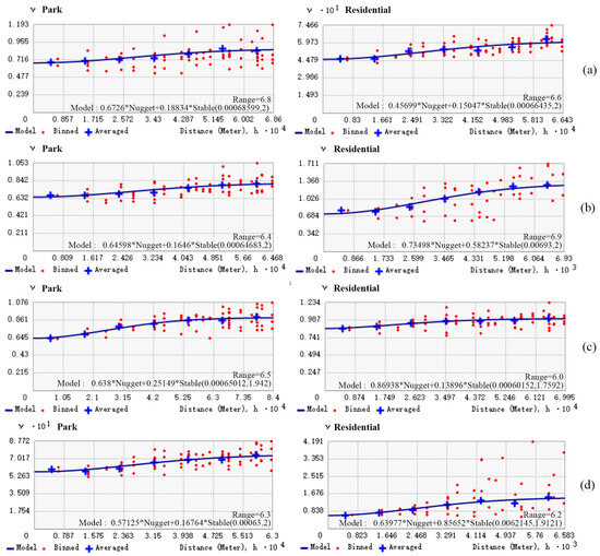
Figure 3.
The final semi variogram model corresponds to the main range of temperature datasets. (a) Summer morning; (b) Summer afternoon; (c) Autumn morning; (d) Autumn afternoon.
We did not build a greater buffer since the research was conducted at the adjacent dimension because an extensive buffer could affect the statistical significance for the temperature data. A similar approach was used for Eduardo Krüger and Baruch Givoni [30]. In ArcGIS 10.8, the average values of BCR, GCR, RD, ISP, WCR, FCR, and Dist_W indicators in different buffers were calculated by using functions such as intersect, field calculator, and summary statistics on aerial photos. In order to overcome the interference of data non-normality, nonlinear relationships and spatial heterogeneity, and to characterize the driving mechanism of the multi-scale thermal environment more robustly. For each spatial scale, the Spearman correlation matrix is used to analyze its correlation with the temperature data to determine the optimal value of each variable for the buffer, and the variable with the highest correlation coefficient is selected as the input for subsequent modeling (Figure 4).
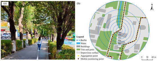
Figure 4.
Photos of the experimental measurement points and buffer zone diagrams. (a) Real photos taken at the measurement points; (b) A series of buffers of the aggregation points of air temperature.
2.5. Model Construction
2.5.1. Multiple Linear Regression
Multiple linear regression is a traditional statistical analysis method that estimates coefficients through the least square method to minimize the sum of squared residuals between predicted and actual values. It is used to explore the linear relationship between multiple independent variables (explanatory variables) and one dependent variable (response variable) and is suitable for analyzing the comprehensive influence of multiple factors on the outcome variable. Its advantage lies in the ability to control confounding variables and quantify the independent contributions of each factor. The main concept is to fit a linear equation to quantify each independent variable’s independent influence on the dependent variable. The formula is as follows:
Among them, represents the dependent variable of the i-th observation, is the intercept term (the reference value when all independent variables are zero), is the regression coefficient of the k-th independent variable, is the value of the k-th independent variable of the i-th observation, and is the random error term (indicating the random fluctuation not captured by the model). The formula ensures logical consistency by fixing the number of independent variables, p.
2.5.2. Machine Learning Models
Machine learning constitutes a scalable nonlinear modeling framework, characterized by adaptive architectures and computationally efficient implementations specifically engineered for deciphering complex relationships in big data environments. This approach augments generalization capacity via consensus mechanisms across constituent models, particularly evident in tree ensembles where combinatorial optimization surpasses individual model limitations [31]. A tree model has several advantages, including excellent comprehension, being able to capture nonlinear trends, suitability for mixed data types, significance of features evaluation, parallel processing support, and the ability to handle large-scale datasets. When distinct models are applied to various datasets, their predicting precision might vary dramatically. By comparing, it is possible to identify the best-performing models in a particular study. In this research, we chose three option tree-based ensemble learning models that typically do well in similar studies to evaluate their results to MLR (Table 4).
Table 4.
Machine learning models.
Samples for the three algorithms (RF, XGBoost, LightGBM)—excluding MLR—were allocated to the training dataset, which was randomly divided into training sets (70%) and test sets (30%). Hyperparameter tuning was conducted independently for each algorithm via grid search with 5-fold cross-validation. These ranges were established based on common practices and recommendations in the machine learning literature [4]. For the Random Forest (RF) model, the hyperparameter mtry was searched over integers 1 to 4; the number of trees was considered from 100 to 500 in increments of 100, and min_n was tested between 2 and 10. For both XGBoost and LightGBM, the number of trees was also selected from 100 to 500 in increments of 100, tree_depth was explored between 3 and 10, and learn_rate was tuned across a continuous range from 0.01 to 0.2. For each algorithm, 10 hyperparameter combinations were evaluated, and the set that yielded the best performance on both R2 and RMSE was selected. The formula for calculating the evaluation metrics is as follows:
where represents the temperature calculated for the ith sample point through different land cover types; represents the predicted data in the prediction results, represents the mean of all the sample sets; and n denotes the number of sample points. Here, R2 is used to represent the extent to which the variation in the dependent variable can be attributed to the independent variable. It varies between 0 and 1, where larger values suggest that the model performs better in accounting for the data’s variability. RMSE assesses the usual variation in errors in prediction, with smaller values suggesting a stronger alignment between expected and observed values. To interpret the model outcomes, the Shapley Additive Explanations (SHAP) method was applied to quantify factor contributions, and Partial Dependency Plots (PDP) were used to visualize threshold effects and nonlinear relationships between key factors and temperature.
3. Results
3.1. Spatial and Temporal Distribution of Air Temperature
Figure 5 and Figure 6 show the temperature changes in the park and outside the park in summer and autumn from the time series and spatial distribution, respectively. In Figure 5, during the morning of summer, the temperature in the park is significantly lower than that in the external residential areas, with a temperature difference of approximately 2.1 °C. This might be consistent with the peaks of vegetation transpiration and the differences in surface heat absorption. However, in residential areas, due to the rapid heat accumulation on ISP, the temperature display keeps rising. In the afternoon, the temperature in the park fluctuates gently, which may be attributed to the buffering effect of water evaporation and vegetation shading. However, in residential areas, due to the heat storage of buildings and the rough underlying surface hindering heat dissipation, the temperature rises sharply, and the cooling rate is about 35% slower than that in the park. During the autumn morning period, the temperature difference between inside and outside the park shrinks to 1.3 °C, and the temperature curve of the park rises slowly, reflecting the regulatory effect of the high specific heat capacity of vegetation and water bodies. Due to the weakened solar radiation, the heating rate in the residential area is only one-third of that in summer. The temperature in the park remained stable in the afternoon. However, the long-wave radiation exchange between the buildings in the residential area delayed the cooling of the residual heat, but the overall temperature difference was significantly greater than that in the park area.
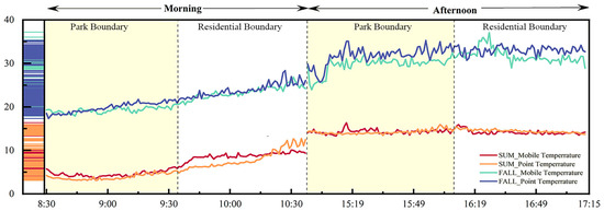
Figure 5.
The temporal variation characteristics of the average temperature, SUM represents the monitoring temperature in summer, and FALL represents the monitoring temperature in autumn.
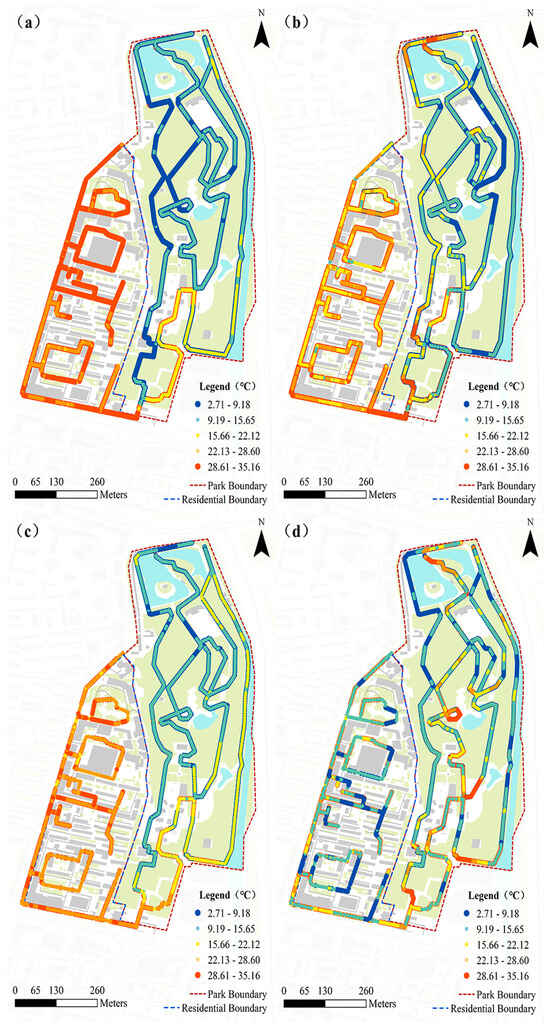
Figure 6.
Spatial distribution of temperature. (a) Summer morning temperature; (b) Summer afternoon temperature; (c) Autumn morning temperature; (d) Autumn afternoon temperature.
Figure 6 shows the spatial distribution of temperatures at different times in summer and autumn. The indoor temperature in the park is significantly lower than that in the residential area in the morning during summer. This might be due to the fact that the peak of vegetation transpiration occurs in the morning, increasing radiation and causing a temperature drop of 6 to 8 degrees Celsius. The high-temperature core areas are concentrated near the residential area roads (29.81–35.16 °C) and in the southwest direction of the residential area (27.04–29.80 °C). The building volume in this area is relatively large, and the artificial heat release may also be higher than that in other areas (Figure 6a). In the afternoon, the temperature in the built-up area remained high. This might be due to the large heat capacity of the concrete material, and the cooling rate of the concrete was slower than that of the park (Figure 6b). The temperature drops in the morning of autumn narrowed. The temperature range in residential areas was lower than that in summer, but the temperature in the park dropped by 3 to 4 degrees Celsius. The park was in a low-temperature area, which might mainly be due to the transfer of natural cooling sources from vegetation to water bodies in autumn, maintaining water evaporation (Figure 6c). In the afternoon, the temperature in the residential area drops (8.99–10.55 °C), which may be suppressed by weakened solar radiation and high wind speeds. The temperature in the park further decreased (6.50–8.98 °C), possibly due to the relatively increased efficiency of water evaporation (Figure 6d). The densely built-up area remains the core area with relatively high temperatures (10.56–14.35 °C), but the average daily temperature difference has narrowed to 4–5 °C compared with summer, indicating that the thermal environment in autumn is greatly affected by the natural cooling of parks, while the influence of urban residential areas has weakened. Overall, the range of high temperatures in summer is relatively wide, and the temperature difference between the two regions is quite obvious. The overall temperature in autumn is relatively low, but spatial differentiation still exists.
3.2. Optimal Buffer
Figure 7 presents the correlation analysis results of temperatures at different time periods in summer and autumn and different buffer zone scales (10–100 m). In terms of the indicators of the park, the correlation of GCR with the change in the buffer zone scale in different time periods is mostly negative. The absolute value of the correlation of some indicators increases at larger buffer zone scales (such as 70 m and 100 m), reflecting that the cooling effect of this indicator strengthens with the expansion of the buffer zone. WCR also shows a similar negative correlation trend, indicating that the regulatory effect of water bodies on temperature is more significant at a larger buffer zone scale. The ISP index can achieve a high correlation in the small-scale buffer zone of 20–40 m in some periods, indicating the local characteristics of the heat accumulation effect of this index. The correlation of RD shows an increasing trend at a larger buffer scale. For residential area indicators, BCR and FCR show a strong correlation in some periods and at a larger buffer zone scale. It is worth noting that the influence degree of BCR in buffer zones of different sizes is only between −0.26 and 0.26, showing a significant difference in the morning and afternoon. It may be positively correlated in the morning due to heat absorption by buildings and negatively correlated in the afternoon due to enhanced shading and ventilation. Overall, the 70 m and 100 m buffers have significantly better temperature interpretation power for most parameters than the small-scale range. Among them, the 100 m buffer covers the inter-zone extremum or sub-extremum of more than 75% of the parameters. Based on the data comparison of summer and autumn in the park area, ISP is the main positively correlated variable. It is positively correlated with temperature in multiple periods and at the buffer zone scale, reflecting the thermal accumulation effect of the impermeable surface. However, GCR and RD are negatively correlated variables. In the large-scale buffer zone, their cooling and regulating effects on temperature are more obvious. WCR shows a negative correlation in the park except in the morning of autumn and is positively correlated in other periods. This might be because the temperature is low in the morning of autumn, the evaporation of water is weak, and the evaporation heat dissipation effect is relatively prominent, taking away the surrounding heat, resulting in a negative correlation. In residential areas, the correlation between ISP and temperature is relatively smaller and more complex than that in parks. This might be because the distribution of ISP in residential areas is more scattered and disturbed by various factors, such as the obstruction of buildings and different building layouts, making the relationship between ISP and temperature not simply positive. The BCR, FCR, and RD in the residential area show obvious temporal differences. In the morning, BCR is positively correlated, and FCR and RD are negatively correlated, and the opposite is true in the afternoon. This might be because during the process of enhanced solar radiation in the morning, the high building density is prone to heat accumulation and temperature rise, while the area with a high FCR is conducive to heat dissipation, and the high road network density is conducive to heat dissipation.
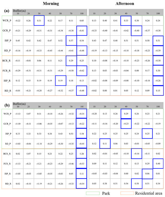
Figure 7.
Spearman’s correlation matrix between park and residential area temperature and different buffer zone radius (10–100 m) indicators in summer and autumn. (a) Summer; (b) Autumn.
3.3. Model Performance Comparison
At the goodness-of-fit level, the research results show that, compared with the MLR model, the performance of the ML model is significantly higher. For example, the value of RF in the residential area in the summer morning is 0.775, and the value of RF in the autumn afternoon is 0.782. It is worth noting that XGBoost and LightGBM perform exceptionally well only at specific times of the day. For instance, XGBoost achieved a performance of 0.746 in the autumn morning park data, while LightGBM’s performance was as high as 0.780, significantly outperforming other models. However, their performance fluctuates, for example, XGBoost dropped to 0.303 in the autumn afternoon park data, and LightGBM dropped to 0.251. The LM performance of the traditional regression model is relatively weak, and its values are generally low. The data of the park in the autumn afternoon is only 0.074. From the perspective of RMSE, the RMSE of the summer afternoon residential data RF is 0.433, and that of the autumn afternoon residential data RF is 0.321, both of which are relatively low values. The RMSE of LightGBM is also generally low. For example, the RMSE of the park data in the summer morning is 0.475. The RMSE of LM is generally high, and the prediction error RMSE of park data in the afternoon of summer reaches 0.801. In terms of computing time, LightGBM and RF have similar training times (2.08–2.85 s), achieving a good balance between accuracy and speed. Combining different results, the RF has more significant advantages (Table 5 and Table 6).
Table 5.
Model performance evaluation—Summer data.
Table 6.
Model Performance Evaluation—Autumn Data.
Considering all aspects comprehensively and on the whole, RF performs well in terms of fitting effect and error index. Therefore, the RF regression model was finally chosen for the subsequent data analysis to analyze the influence of urban morphology on the temperature distribution. It builds multiple independent decision trees by randomly selecting training samples and predictors and then generates the final predicted value using a combined strategy. It can not only utilize the nonlinear fitting ability of the decision tree but also effectively reduce the risk of overfitting through the randomization mechanism. Improving the generalization performance of the model can better adapt to the data characteristics and analysis requirements of this study.
3.4. Identification of Dominant Driving Factors
In our study, the SHAP values were derived from independent models for each season and were not normalized across seasons. This approach aligns with common practices [13] in explainable machine learning for environmental studies, where the primary focus is on interpreting relative feature rankings within specific models or contexts, rather than comparing absolute SHAP magnitudes across them. Figure 8a,b, respectively, show the analysis results of the importance of temperature influencing factors in parks and residential areas in the morning and afternoon of summer and autumn. This method takes all samples into account and calculates the average absolute SHAP value of each feature. The local significance is illustrated on the left side by showing the SHAP value of each feature of each sample. This highlights the most crucial features and demonstrates the extent to which they affect the dataset. In this visualization, the Y-axis corresponds to the feature, while the X-axis represents the SHAP value. The positive value of the bee colony graph on the right indicates an increase in the prediction result, while a negative value indicates a decrease.
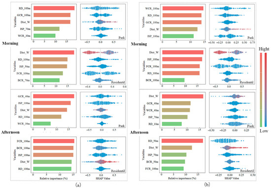
Figure 8.
The SHAP values of different influencing factors of parks and residential areas on temperature in the RF model; (a) Summer; (b) Autumn.
The results show that in the park area on summer mornings, RD has the greatest influence on temperature, followed by GCR and Dist_W. It can be observed from the bee colony map that the influences of GCR and RD on temperature have a certain negative distribution range, while the SHAP value of Dist_W is large and mainly positive, indicating that the farther the water body distance, the higher the temperature. In residential communities, Dist_W has the most significant influence on temperature, followed by RD, ISP, and FCR. The bee colony map shows that Dist_W has a significant negative impact on temperature, contrary to the park area. This indicates that in residential areas, the farther away from water bodies, the lower the temperature may be. The positive influence of BCR on temperature is relatively small. In the afternoon, the ISP and GCR of the park became the main influencing factors, while the RD and FCR of the residential area had a greater impact. In the park area in the autumn morning, WCR has the greatest impact on temperature, followed by RD and GCR. The bee colony map shows that WCR and GCR have a significant negative impact on temperature, indicating that the water body and green coverage in the park area have a positive effect on cooling. In residential areas, the factor that has the greatest impact on temperature is Dist_W, followed by ISP and FCR. The colony map shows that Dist_W is positively affecting the temperature, while the effects of ISP and FCR are relatively neutral. In the afternoon period, the influence of Dist_W and GCR in the park area is relatively large, while the influence of RD is relatively neutral.
3.5. Partial Dependence and Threshold Effects of Driving Factors
In order to clarify the sensitivity of these factors and determine the optimal threshold for the cooling effect. The partial dependence between different regional driving factors and summer temperatures is shown in Figure 9. In the park during the summer morning, the temperature of ISP is relatively stable at a lower value and then rises rapidly. Controlling ISP is crucial, as temperature remains low but rises rapidly beyond a certain point. The temperature drops significantly when RD exceeds 3. The temperature is stable when GCR is lower than approximately 40% and fluctuates after exceeding this threshold. Green coverage shows a stable cooling effect up to approximately 40%, beyond which temperature fluctuations increase, establishing this value as a critical benchmark for reliable green space cooling. WCR shows a roughly linear positive relationship with temperature, and the strength of this correlation fluctuates within a specific range. In the summer afternoon, the temperature of ISP keeps rising with the increase in value. RD rises between 2 and 4 and decreases after exceeding 4, revealing an optimal road density range that balances infrastructure needs with thermal comfort. The temperature of Dist_W keeps rising with the increase in value, highlighting the importance of proximity to water bodies for effective cooling. GCR fluctuates significantly between 0.5 and 1. The temperature of WCR keeps rising with the increase in value. In the community, during the summer morning, the temperature of ISP is relatively high when it is around 0 to 0.25, then decreases and rises rapidly after 0.5, showing a pattern of first decreasing and then increasing. The temperature of RD decreases significantly between 2 and 4 and tends to stabilize after exceeding 4. The temperature of Dist_W continues to decrease as the value increases, providing a quantitative basis for integrating water features into community design. The BCR first decreases and then increases between 10 and 30. When the FCR is below 1, temperature drops rapidly and stabilizes beyond 1, offering a clear threshold for regulating built volume to mitigate heat accumulation (Figure 9).
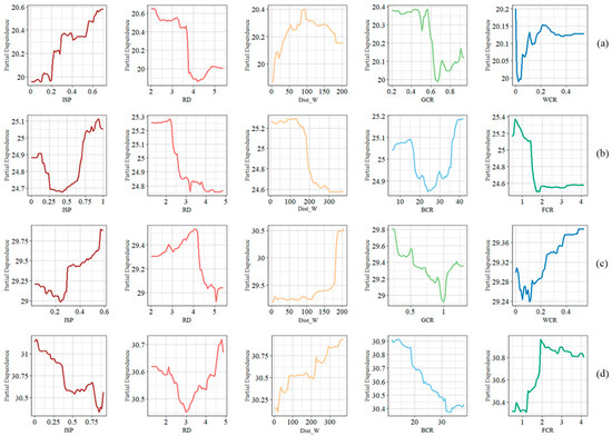
Figure 9.
The partial dependence of influencing factors and summer temperatures, (a) Morning Park; (b) Morning Residential Area; (c) Afternoon Park; (d) Afternoon Residential Area.
In the park, when the ISP is low in the autumn morning, the temperature is stable and then rises rapidly. After RD exceeds 3, the temperature drops significantly, indicating that this threshold may similarly promote beneficial airflow in the autumn season. When GCR is lower than 0.2, the temperature is stable and fluctuates beyond the threshold, proposing a potential lower benchmark for green space efficacy in autumn compared to summer. In the afternoon, the temperature of ISP continued to rise as the value increased. RD fluctuated and rose from 0 to 5 and decreased beyond 5, suggesting an optimal upper threshold for RD to avoid afternoon heat retention. The temperature continued to rise as the Dist_W value increased, reinforcing the year-round cooling benefit of proximity to water bodies. GCR fluctuated from 0.5 to 1. The temperature continued to rise as the WCR value increased. In the morning of autumn in the residential area, the ISP has a high temperature ranging from 0 to 0.25, then drops, and then rises rapidly after 0.5. The RD has a significant temperature drop between 2 and 4 and tends to stabilize above 4, supporting the consistent role of moderate road density in facilitating cooling across seasons. The BCR first drops and then rises between 10 and 40. FCR drops rapidly at temperatures below 1 and tends to stabilize above 1, echoing the summer findings and underscoring FCR’s consistent role in thermal regulation. In the afternoon, the temperature of ISP continued to decrease as the value increased. RD shows a temperature increase between 2 and 6, decreasing beyond 6, implying a higher optimal road density threshold for autumn afternoons to maximize ventilation. The temperature continued to rise as the Dist_W value increased. BCR first decreased and then fluctuated between 10 and 50. FCR rose rapidly below 1 and fluctuated and decreased above 1. These patterns demonstrate distinct time-specific threshold effects of key parameters on temperature across different spatial types during autumn, providing critical insights for seasonally informed urban design (Figure 10).
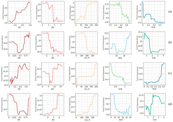
Figure 10.
The partial dependence of influencing factors and autumn temperatures, (a) Morning Park; (b) Morning Residential Area; (c) Afternoon Park; (d) Afternoon Residential Area.
4. Discussion
4.1. Differences in Optimal Spatial Scales and Variations in Ideal Spatial Scales
Due to the significant differences in temperature caused by different influencing factors, many studies determined the optimal buffer size before the start of the research and believed that different buffer sizes had a significant impact on machine learning models [32]. The size and shape of the buffer zone can affect the research results and may explain some inconsistent findings in the environment and energy balance [33]. Compared with the existing studies that mostly focus on a single season or a fixed buffer zone scale [34]. Many studies have also compared and classified the buffers of different types of factors. In Changchun City, the three-dimensional index is more accurate in predicting the temperature at the 500 m scale than the two-dimensional index, while the two-dimensional index has a more significant impact on the 1000 m scale [35]. In Shanghai, a 100 m buffer zone is regarded as the best choice for testing the temperature influence factor [36]. Similarly to the study in [37], this study found that in different study regions, the regulatory effects of each influencing factor on temperature showed significant differences in scale, period, and season. The regional impact factor of residential areas has a relatively large mesoscale influence in some cases, which may also be related to the significant “three-dimensional heat transfer” characteristics in modern buildings proposed by Gao et al. The influence of architectural form indicators needs to be evaluated within the mesoscale range [29]. In the park indicators, with the expansion of the buffer zone, the cooling effects of GCR and WCR increase significantly, indicating that the cooling capacity of natural cold sources needs to be achieved through spatial continuity [38]. This is highly consistent with the planning principle of wide-area vegetation-water body connection in the “Cold Island Network” theory [39]. It is notable that as the buffer zone expands, the negative correlation of RD increases significantly, reflecting that the cumulative effect of traffic heat emissions during the hot season dominates the deterioration of the thermal environment. However, in autumn, there is a certain degree of fluctuation, which is different from the regular increase in summer. This might indicate that the intensity of the artificial heat source decreases during the low-temperature period, and the degree of temperature drop varies with the traffic cycle or is caused by other complex factors [40]. Furthermore, the 70 m and 100 m buffer layers have the best interpretive ability for most parameters (covering 75% of the parameter extremums), and some research conclusions are consistent with this paper. They found that the larger the buffer size, the better the cooling effect [41]. Under the interaction of the thermal environment regulation mechanism, a complex thermal regulation system is formed, resulting in significant differences in the correlation intensities of temperature drivers in different buffer zones.
4.2. Comparison of Models
Both MLR and ML offer adaptability and convenience tailored to specific scenarios. This research examined the relationship between the influencing factor and temperature by employing the MLR model along with three machine learning models. Despite being developed using the same dataset, these models exhibited notable variations in performance. Our optimal model, Random Forest (RF), consistently achieved R2 values ranging from 0.531 to 0.775, while the RMSE remained below 0.6. This level of performance is comparable to that reported in related studies. For instance, a previous research report that used LightGBM as the optimal model for temperature prediction stated that its R2 value was approximately 0.57 and the RMSE value was 1.27 [13]. In another example, a study that applied XGBoost achieved an R2 value as high as 0.73–0.96 [42]. Furthermore, another study that applied the RF model in different indicators of the same region showed a difference of around 0.28 in R2 values, while the RMSE values ranged from 0.35 to 0.92 [43]. It is also worth exploring how applicable these models are in various scenarios. These inherent characteristics make each model particularly suited to different types of data features. The predictive frameworks established, particularly those of the tree-based models, are likely transferable to other cities in principle, as the key drivers of urban temperature are universally relevant. However, the specific impact and optimal thresholds of factors such as GCR or RD are context-dependent and may vary under different climatic conditions. For example, the cooling effect of vegetation is likely more pronounced in humid regions than in arid ones, and the optimal RD for maximizing ventilation may depend on background wind patterns. Therefore, while our models demonstrate high predictive accuracy within the study area, their direct application to cities with fundamentally different climates requires caution and local calibration. Future work should prioritize validating these models across diverse climatic zones to thoroughly assess their robustness and broaden their applicability.
4.3. Divergent Dominant Factors Across Regions
Through the analysis of SHAP and PDP in this study, it was found that the spatiotemporal variation patterns of temperature in autumn and summer in individual periods showed some similarities, but there were significant differences in the dominant factors and threshold effects of thermal drive in different regions. This is similar to the research of [44]. Whether it is a park or a residential area, RD and Dist_W are the leading factors in the ranking of thermal driving factors most of the time, especially in autumn. This is consistent with the conclusions in [45] regarding the continuous influence of traffic heat sources in summer and [46], that the evaporative cooling efficiency of water bodies is rapidly released after sunrise under the low-temperature conditions in the early morning of autumn. However, the secondary dominant factors show significant temporal differentiation. In the morning in the park, GCR and ISP dominate the changes in the thermal environment. The PDP curve reveals that when GCR > 75%, the cooling efficiency tends to be saturated (with a slope decrease of 58%), while for every 10% increase in ISP, the temperature rises by 0.05 °C, and when ISP is greater than 50%, the influence weakens [47]. This is consistent with the “vegetation transpiration-surface radiation competition mechanism” proposed in the study [48]. Compared with the study of humid cities [47] in Jiangsu, the heat contribution rate of ISP in arid areas is 23% higher, and the lower cooling effect is concentrated in arid areas [49]. Under the synergistic effect of WCR, the heat regulation efficiency of limited water bodies in arid areas is highlighted [50]. The FCR in the residential area was significant in the afternoon period, which is consistent with the ventilation efficiency threshold theory of due to the difference in building height [51].
4.4. Practical Implications for the Planning of Areas Adjacent to Urban Parks
Coordinating the relationships among various elements of urban parks and adjacent residential areas, exploring the interaction mechanisms among different elements with the goal of maximizing the cooling effect, and forming an optimized layout model of coordination among small areas is conducive to helping urban construction adapt to the climate conditions of improved thermal environment, achieving a win-win effect of alleviating the UHI and ensuring the physical health of residents. Combined with the analysis of the contribution degree and threshold effect of various influencing factors of the park and the surrounding residential areas on temperature in the previous text, the optimization strategies for the design elements of the park and the adjacent residential areas are proposed to enhance the operability of the optimized layout of the park. Especially for cities in arid areas, targeted planning strategies are needed, which is an important method to achieve the sustainable development goals [52]. When there are high-rise buildings around the park, the overlapping shadow shading of the buildings themselves can provide moderate cooling. Based on the previous research and analysis, for every 50% reduction in FCR, through the superimposed effect of constructing three-dimensional shading and thermal inertia, the temperature in the summer morning may decrease by 0.15 degrees Celsius. However, when the BCR in the buffer zone exceeds 35%, its insulation effect leads to a temperature increase of 0.2–0.3 degrees Celsius. Similarly to other studies, when the height of the building increased from 12 m to 72 m, the temperature dropped by approximately 1.7 °C [53]. When the land use is suitable, BCR and FCR should be planned in a coordinated manner. The FCR can be appropriately increased by covering with three-dimensional shadows and enhancing ventilation to counteract the UHI of high-density development, but the insulation effect caused by overly dense buildings should be avoided. But the surrounding areas of the water body need to coordinate BCR and FCR to avoid high-rise buildings blocking the evaporative cooling efficiency of the water body. In terms of sustainability, based on the enhancement effect of GCR in the large buffer zone, green corridors need to be designed to link different green areas and open spaces throughout the city, creating an uninterrupted green system. Such as a new method for connecting cold islands mentioned in the Quan & Li study: Face (cooling sources)-line (networks)-point (cooling spaces, heating spaces). Apply circuit theory to construct the cooling network and identify key nodes, enhance the connectivity of cooling sources, implement effective cooling measures in key node areas, and control the density of buildings and branches at the block scale [39]. The adopted method can provide new ideas for urban sustainable development and urban climate adaptation planning.
4.5. Prospects and Limitations
This study still has the following several limitations. Firstly, although the random forest regression method effectively reveals the nonlinear relationship between the influence factors and temperature in the two areas of parks and residential areas, and the model accuracy is better than that of the traditional linear regression method, the currently constructed influence factor index system still needs to be deepened. This study focuses on seven typical influencing factors, emphasizing the quantification of the influence mechanism of each factor in different spatial utilization characteristics on temperature. However, the influencing factors of temperature are multi-dimensional and complex. For instance, the canopy shading capacity of the vegetation community structure, key parameters such as the ventilation effect of the three-dimensional form of buildings, and the albedo characteristics of surface materials have not yet been incorporated into the assessment system. In the future, it is necessary to integrate multi-source data such as 3D models and hyperspectral remote sensing to construct a more refined thermal environment coupling index system. Secondly, the empirical analysis of this study focused on typical parks and adjacent communities. Although the reliability of the conclusion was guaranteed through high-precision microclimate monitoring data, the morphological characteristics of a single case were difficult to fully represent the heterogeneity of the entire urban system. Limited by the difficulty in obtaining large-scale continuous meteorological observation data, the subsequent study intends to combine the thermal infrared data of Sentinel-2/3 satellites with the mobile monitoring network of unmanned aerial vehicles to construct a multi-level observation system of “macro-meso-micro,” revealing the influence laws of different factors on temperature under the background of different urban functional areas and climate zones in a more systematic way, enhancing the universal value of the research conclusions.
5. Conclusions
This study selected representative parks and adjacent residential areas in Urumqi, a typical oasis city in an arid area, during the summer and autumn of 2023 as the research objects. A mobile monitoring experiment was designed to obtain temperature data as the dependent variable, and different influencing factors were selected as independent variables according to the regional division characteristics. The optimal index of the buffer zone was selected as the parameter of the machine learning model. Finally, the RF model was chosen to continue the SHAP interpretable analysis. The linear and nonlinear influence mechanisms of the influencing factors on temperature under different land use areas were studied, including feature importance and marginal effect. The following is the research conclusion: (1) The spatiotemporal distribution of temperature in parks and residential areas shows significant differences at different times. In the comparison of multi-scenario data, the larger the buffer zone, the better the fitting effect with temperature. (2) The RF model is the best model for temperature prediction in People’s Park and its adjacent areas. (3) In the park area, GCR and RD play a dominant role, while in the residential area, Dist_W is the main driving factor, and its influence on temperature in the morning and afternoon shows opposite trends. (4) There is a significant time-limit threshold effect on the influence of key parameters of parks and residential areas on temperature. It is suggested that in the urban spatial layout, differentiated planning should be carried out for different utilization spaces while considering the synergy effect. For example, the areas around the water bodies in urban parks need to coordinate BCR and FCR to avoid high-rise buildings hindering the evaporative cooling efficiency of the water bodies. As for green spaces, based on the enhanced effect in the large buffer zone, it is recommended to connect different green open spaces. These findings offer new insights into temperature drivers and provide references for effectively regulating urban ecosystems, which can help alleviate extreme high-temperature events in cities.
Author Contributions
Conceptualization, Y.F. and X.C.; methodology, Y.F. and S.X.; software, Y.F. and S.X.; validation, Y.F. and X.C.; formal analysis, Y.F.; data curation, Y.F.; writing—original draft preparation, Y.F.; writing—review and editing, Y.F.; visualization, Y.F.; supervision, X.C.; funding acquisition, X.C. All authors have read and agreed to the published version of the manuscript.
Funding
The research was sponsored by the Natural Science Foundation of Xinjiang Uygur Autonomous Region (2022D01A212) and the National Science Foundation of China [No. 41861033].
Institutional Review Board Statement
Not applicable.
Informed Consent Statement
Not applicable.
Data Availability Statement
The original contributions presented in the study are included in the article, further inquiries can be directed to the corresponding author.
Conflicts of Interest
The authors declare no competing interests.
References
- United Nations Sustainable Development Goals Report. Available online: https://www.un.org/sustainabledevelopment/es/cities/ (accessed on 25 July 2025).
- Tuholske, C.; Caylor, K.; Funk, C.; Verdin, A.; Sweeney, S.; Grace, K.; Peterson, P.; Evans, T. Global urban population exposure to extreme heat. Proc. Natl. Acad. Sci. USA 2021, 118, e2024792118. [Google Scholar] [CrossRef]
- Zhang, X.; Estoque, R.C.; Murayama, Y. An urban heat island study in Nanchang City, China based on land surface temperature and social-ecological variables. Sustain. Cities Soc. 2017, 32, 557–568. [Google Scholar] [CrossRef]
- Arnett, E.B.; Hein, C.D.; Schirmacher, M.R.; Huso, M.M.; Szewczak, J.M. Evaluating the Effectiveness of an Ultrasonic Acoustic Deterrent for Reducing Bat Fatalities at Wind Turbines. PLoS ONE 2013, 8, e65794. [Google Scholar] [CrossRef]
- Nasrollahpour, R.; Skorobogatov, A.; He, J.; Valeo, C.; Chu, A.; van Duin, B. The impact of vegetation and media on evapotranspiration in bioretention systems. Urban For. Urban Green. 2022, 74, 127680. [Google Scholar] [CrossRef]
- Jiacheng, F.; Yupeng, W.; Dian, Z.; Shi-Jie, C. Impact of Urban Park Design on Microclimate in Cold Regions using newly developped prediction method. Sustain. Cities Soc. 2022, 80, 103781. [Google Scholar] [CrossRef]
- Wang, L.; Wang, W.; Tang, F.; Xu, H. Optimizing urban park cooling effects requires balancing morphological design and landscape structure. Sci. Rep. 2025, 15, 15435. [Google Scholar] [CrossRef]
- Kousis, I.; Pigliautile, I.; Pisello, A.L. Intra-urban microclimate investigation in urban heat island through a novel mobile monitoring system. Sci. Rep. 2021, 11, 9732. [Google Scholar] [CrossRef] [PubMed]
- Martins Gnecco, V.; Pigliautile, I.; Pisello, A.L. Long-Term Thermal Comfort Monitoring via Wearable Sensing Techniques: Correlation between Environmental Metrics and Subjective Perception. Sensors 2023, 23, 576. [Google Scholar] [CrossRef] [PubMed]
- Xu, H.; Chen, H.; Zhou, X.; Wu, Y.; Liu, Y. Research on the relationship between urban morphology and air temperature based on mobile measurement: A case study in Wuhan, China. Urban Clim. 2020, 34, 100671. [Google Scholar] [CrossRef]
- García-Santos, V.; Sánchez, J.; Cuxart, J. Evapotranspiration Acquired with Remote Sensing Thermal-Based Algorithms: A State-of-the-Art Review. Remote Sens. 2022, 14, 3440. [Google Scholar] [CrossRef]
- Wang, X.; Rahman, M.A.; Mokroš, M.; Rötzer, T.; Pattnaik, N.; Pang, Y.; Zhang, Y.; Da, L.; Song, K. The influence of vertical canopy structure on the cooling and humidifying urban microclimate during hot summer days. Landsc. Urban Plan. 2023, 238, 104841. [Google Scholar] [CrossRef]
- Wang, Z.; Zhou, R.; Rui, J.; Yu, Y. Revealing the impact of urban spatial morphology on land surface temperature in plain and plateau cities using explainable machine learning. Sustain. Cities Soc. 2025, 118, 106046. [Google Scholar] [CrossRef]
- Anqi, Z.; Chang, X.; Weifeng, L. Relationships between 3D urban form and ground-level fine particulate matter at street block level: Evidence from fifteen metropolises in China. Build. Environ. 2022, 211, 108745. [Google Scholar] [CrossRef]
- Gongbo, C.; Shanshan, L.; Luke, D.K.; Hamm, N.A.S.; Wei, C.; Tiantian, L.; Jianping, G.; Hongyan, R.; Michael, J.A.; Yuming, G. A machine learning method to estimate PM2.5 concentrations across China with remote sensing, meteorological and land use information. Sci. Total Environ. 2018, 636, 52–60. [Google Scholar]
- Komeh, Z.; Hamzeh, S.; Memarian, H.; Attarchi, S.; Alavipanah, S.K. A Remote Sensing Approach to Spatiotemporal Analysis of Land Surface Temperature in Response to Land Use/Land Cover Change via Cloud Base and Machine Learning Methods, Case Study: Sari Metropolis, Iran. Int. J. Environ. Res. 2025, 19, 98. [Google Scholar] [CrossRef]
- Tanoori, G.; Soltani, A.; Modiri, A. Machine Learning for Urban Heat Island (UHI) Analysis: Predicting Land Surface Temperature (LST) in Urban Environments. Urban Clim. 2024, 55, 101962. [Google Scholar] [CrossRef]
- McCarty, D.; Lee, J.; Kim, H.W. Machine Learning Simulation of Land Cover Impact on Surface Urban Heat Island Surrounding Park Areas. Sustainability 2021, 13, 12678. [Google Scholar] [CrossRef]
- Sun, Y.; Gao, C.; Li, J.; Gao, M.; Ma, R. Assessing the cooling efficiency of urban parks using data envelopment analysis and remote sensing data. Theor. Appl. Climatol. 2021, 145, 903–916. [Google Scholar] [CrossRef]
- ElTaweel, M.H.; Alfaro, S.C.; Siour, G.; Coman, A.; Robaa, S.M.; Wahab, M.M.A. Prediction and forecast of surface wind using ML tree-based algorithms. Meteorol. Atmos. Phys. 2023, 136, 1. [Google Scholar] [CrossRef]
- Gu, X.; Zhang, J. Green and grey cooling: Mitigating pedestrians perceived temperature via urban shades. Build. Environ. 2025, 285, 113585. [Google Scholar] [CrossRef]
- Tsin, P.K.; Knudby, A.; Krayenhoff, E.S.; Ho, H.C.; Brauer, M.; Henderson, S.B. Microscale mobile monitoring of urban air temperature. Urban Clim. 2016, 18, 58–72. [Google Scholar] [CrossRef]
- Lam, C.K.C.; Alnaqshabandy, H.; Lewin, S.; Morewood, J.; Xie, X.; Goodhew, S. Making intra-urban monitoring ‘a walk in the park’: A mobile monitoring approach for assessing pedestrians’ environmental conditions. Build. Environ. 2025, 284, 113487. [Google Scholar] [CrossRef]
- Kousis, I.; Pigliautile, I.; Pisello, A.L. Investigating the intra-urban thermal and air quality environment: New transect sensing methodology and measurements. Measurement 2023, 219, 113210. [Google Scholar] [CrossRef]
- Huang, C.; Hu, T.; Duan, Y.; Li, Q.; Chen, N.; Wang, Q.; Zhou, M.; Rao, P. Effect of urban morphology on air pollution distribution in high-density urban blocks based on mobile monitoring and machine learning. Build. Environ. 2022, 219, 109173. [Google Scholar] [CrossRef]
- Rivera, M.; Basagaña, X.; Aguilera, I.; Agis, D.; Bouso, L.; Foraster, M.; Medina-Ramón, M.; Pey, J.; Künzli, N.; Hoek, G. Spatial distribution of ultrafine particles in urban settings: A land use regression model. Atmos. Environ. 2012, 54, 657–666. [Google Scholar] [CrossRef]
- Liu, Y.; Fan, J.; Xie, S.; Chen, X. Study on the Spatial and Temporal Distribution of Thermal Comfort and Its Influencing Factors in Urban Parks. Atmosphere 2024, 15, 183. [Google Scholar] [CrossRef]
- Ferreira, L.S.; Duarte, D.H.S. Exploring the relationship between urban form, land surface temperature and vegetation indices in a subtropical megacity. Urban Clim. 2019, 27, 105–123. [Google Scholar] [CrossRef]
- Fan, J.; Chen, X.; Xie, S.; Du, K. Mediating effect of air pollutants on urban morphology and air temperature. Atmos. Pollut. Res. 2025, 16, 102426. [Google Scholar] [CrossRef]
- Yan, H.; Fan, S.; Guo, C.; Hu, J.; Dong, L. Quantifying the Impact of Land Cover Composition on Intra-Urban Air Temperature Variations at a Mid-Latitude City. PLoS ONE 2014, 9, e102124. [Google Scholar] [CrossRef] [PubMed]
- Ulpiani, G. On the linkage between urban heat island and urban pollution island: Three-decade literature review towards a conceptual framework. Sci. Total Environ. 2020, 751, 141727. [Google Scholar] [CrossRef]
- Liu, X.; Chen, X.; Tian, M.; De Vos, J. Effects of buffer size on associations between the built environment and metro ridership: A machine learning-based sensitive analysis. J. Transp. Geogr. 2023, 113, 103730. [Google Scholar] [CrossRef]
- James, P.; Berrigan, D.; Hart, J.E.; Aaron Hipp, J.; Hoehner, C.M.; Kerr, J.; Major, J.M.; Oka, M.; Laden, F. Effects of buffer size and shape on associations between the built environment and energy balance. Health Place 2014, 27, 162–170. [Google Scholar] [CrossRef]
- Yang, Z.; Chen, Y.; Zheng, Z.; Huang, Q.; Wu, Z. Application of building geometry indexes to assess the correlation between buildings and air temperature. Build. Environ. 2020, 167, 106477. [Google Scholar] [CrossRef]
- Zhang, J.; Li, Z.; Hu, D. Effects of urban morphology on thermal comfort at the micro-scale. Sustain. Cities Soc. 2022, 86, 104150. [Google Scholar] [CrossRef]
- Yang, C.; Kui, T.; Zhou, W.; Fan, J.; Pan, L.; Wu, W.; Liu, M. Impact of refined 2D/3D urban morphology on hourly air temperature across different spatial scales in a snow climate city. Urban Clim. 2023, 47, 101404. [Google Scholar] [CrossRef]
- Liu, Y.; Zhang, W.; Liu, W.; Tan, Z.; Hu, S.; Ao, Z.; Li, J.; Xing, H. Exploring the seasonal effects of urban morphology on land surface temperature in urban functional zones. Sustain. Cities Soc. 2024, 103, 105268. [Google Scholar] [CrossRef]
- Zhou, D.; Bonafoni, S.; Zhang, L.; Wang, R. Remote sensing of the urban heat island effect in a highly populated urban agglomeration area in East China. Sci. Total Environ. 2018, 628-629, 415–429. [Google Scholar] [CrossRef] [PubMed]
- Qian, W.; Li, X. A cold island connectivity and network perspective to mitigate the urban heat island effect. Sustain. Cities Soc. 2023, 94, 104525. [Google Scholar] [CrossRef]
- Teufel, B.; Sushama, L.; Poitras, V.; Dukhan, T.; Bélair, S.; Miranda-Moreno, L.; Sun, L.; Sasmito, A.P.; Bitsuamlak, G. Impact of COVID-19-Related Traffic Slowdown on Urban Heat Characteristics. Atmosphere 2021, 12, 243. [Google Scholar] [CrossRef]
- Gao, J.; Gong, J.; Yang, J.; Li, J.; Li, S. Measuring Spatial Connectivity between patches of the heat source and sink (SCSS): A new index to quantify the heterogeneity impacts of landscape patterns on land surface temperature. Landsc. Urban Plan. 2022, 217, 104260. [Google Scholar] [CrossRef]
- Chen, S.; Feng, Y.; Guan, C.; Xu, Y.; Tan, Q.; Li, Y.; Yang, X. Machine learning approaches to predicting urban park attractiveness: Insights from Shanghai and Tokyo. Urban For. Urban Green. 2025, 112, 128921. [Google Scholar] [CrossRef]
- Han, L.; Zhao, J.; Gao, Y.; Gu, Z. Prediction and evaluation of spatial distributions of ozone and urban heat island using a machine learning modified land use regression method. Sustain. Cities Soc. 2022, 78, 103643. [Google Scholar] [CrossRef]
- Kammuang-Lue, N.; Sakulchangsatjatai, P.; Sangnum, P.; Terdtoon, P. Influences of population, building, and traffic densities on urban heat island intensity in Chiang Mai City, Thailand. Therm. Sci. 2015, 19, 445–455. [Google Scholar] [CrossRef]
- Elmarakby, E.; Elkadi, H. Impact of urban morphology on Urban Heat Island in Manchester’s transit-oriented development. J. Clean. Prod. 2023, 434, 140009. [Google Scholar] [CrossRef]
- Wen, C.; Mamtimin, A.; Feng, J.; Wang, Y.; Yang, F.; Huo, W.; Zhou, C.; Li, R.; Song, M.; Gao, J.; et al. Diurnal Variation in Urban Heat Island Intensity in Birmingham: The Relationship between Nocturnal Surface and Canopy Heat Islands. Land 2023, 12, 2062. [Google Scholar] [CrossRef]
- Wang, Y.; Li, X.; Zhang, C.; He, W. Influence of spatiotemporal changes of impervious surface on the urban thermal environment: A case of Huai’an central urban area. Sustain. Cities Soc. 2022, 79, 103710. [Google Scholar] [CrossRef]
- Duveiller, G.; Hooker, J.; Cescatti, A. The mark of vegetation change on Earth’s surface energy balance. Nat. Commun. 2018, 9, 679. [Google Scholar] [CrossRef] [PubMed]
- Wang, C.; Ren, Z.; Dong, Y.; Zhang, P.; Guo, Y.; Wang, W.; Bao, G. Efficient cooling of cities at global scale using urban green space to mitigate urban heat island effects in different climatic regions. Urban For. Urban Green. 2022, 74, 127635. [Google Scholar] [CrossRef]
- Steeneveld, G.J.; Koopmans, S.; Heusinkveld, B.G.; Theeuwes, N.E. Refreshing the role of open water surfaces on mitigating the maximum urban heat island effect. Landsc. Urban Plan. 2014, 121, 92–96. [Google Scholar] [CrossRef]
- Peng, J.; Liu, Q.; Xu, Z.; Lyu, D.; Du, Y.; Qiao, R.; Wu, J. How to effectively mitigate urban heat island effect? A perspective of waterbody patch size threshold. Landsc. Urban Plan. 2020, 202, 103873. [Google Scholar] [CrossRef]
- Bavnbæk, K.F.; Thuesen, A.A. Navigating spatial justice: Exploring municipal planners’ logics in differentiated village planning. J. Rural. Stud. 2024, 114, 103496. [Google Scholar] [CrossRef]
- Li, J.; Zheng, B.; Bedra, K.B.; Li, Z.; Chen, X. Effects of residential building height, density, and floor area ratios on indoor thermal environment in Singapore. J. Environ. Manag. 2022, 313, 114976. [Google Scholar] [CrossRef] [PubMed]


Disclaimer/Publisher’s Note: The statements, opinions and data contained in all publications are solely those of the individual author(s) and contributor(s) and not of MDPI and/or the editor(s). MDPI and/or the editor(s) disclaim responsibility for any injury to people or property resulting from any ideas, methods, instructions or products referred to in the content. |
© 2025 by the authors. Licensee MDPI, Basel, Switzerland. This article is an open access article distributed under the terms and conditions of the Creative Commons Attribution (CC BY) license (https://creativecommons.org/licenses/by/4.0/).