Abstract
To improve the efficiency and accuracy of steel surface defect detection while reducing computational complexity, this paper proposes a lightweight detection algorithm—Finite Element Method-YOLO (FEM-YOLO). The algorithm aims to enhance defect detection performance by optimizing the network architecture and minimizing computational overhead. Methodologically, FEM-YOLO is based on the YOLOv8n architecture, incorporating a lightweight Feature Net network as the backbone for feature extraction. Through efficient parameter sharing and feature extraction mechanisms, the algorithm reduces its complexity. Additionally, FEM-YOLO innovatively combines Enhance Conv with the C2f module to form the C2f-Enhance module, thereby improving the representation of fine details and edges within the feature maps. To further enhance detection performance, a multi-path shared convolutional detection head is designed. This design significantly reduces the number of parameters through parameter sharing, thereby improving detection accuracy while maintaining the lightweight nature of the algorithm. The experimental results demonstrate that, on the NEU-DET enhanced dataset, the FEM-YOLO algorithm achieves a parameter count of 1.4 M, which is reduced to 43.7% of the baseline algorithm, with a computational complexity of 4.6 GFLOPs, 52.9% lower than the baseline. Furthermore, the FPS reaches 256. When employing the Focal_EIoU loss function, the mean Average Precision (mAP) reaches 83.3%, validating the algorithm’s efficiency and accuracy in steel surface defect detection.
1. Introduction
Steel strips are a core product in the iron and steel industry, widely used in fields such as automotive manufacturing, mechanical engineering, chemical equipment, and aerospace. Over the past decade, the production process technology of steel strips has achieved significant improvements, particularly in aspects of thickness, material quality, and shape [1,2]. However, with the increasing quality requirements for steel strips in high-end industries, the occurrence of surface defects (such as scratches and inclusions) remains unavoidable, which seriously affects production efficiency and product quality [3]. Therefore, the detection of steel strip surface defects has become a key factor in ensuring product quality.
Currently, defect detection methods are mainly divided into three categories: traditional methods (e.g., manual sampling, infrared detection, and magnetic particle detection), machine vision-based detection, and deep learning-based detection technologies [4]. The limitation of traditional methods lies in their relatively large detection errors; although machine vision methods have achieved improvements, they still have shortcomings in multi-type defect classification and real-time performance [5]. Deep learning technologies, especially object detection technologies, have made significant progress in industrial applications, enhancing detection accuracy and efficiency [6,7].
Kou et al. [8] applied the YOLOv3 algorithm to the thin steel surface defect image dataset NEU-DET, achieving an average precision (mAP) of 72.2%, confirming the suitability of YOLOv3 for thin steel surface defect detection. Cheng and Yu [9] proposed a RetinaNet algorithm combining attention mechanisms and adaptive spatial feature fusion modules, which effectively improved defect detection performance on thin steel surfaces. Li et al. [10] introduced an improved YOLOv5 network algorithm for small surface defects, incorporating a Convolutional Block Attention Module (CBAM) and optimizing the network architecture and loss function, achieving an average precision (mAP) of 91.0% on a self-constructed industrial defect dataset. Furthermore, Chen et al. [11] proposed a fast thin steel surface defect detection network (DCAM-Net) based on deformable convolutions and attention mechanisms, significantly enhancing the network’s localization capability. This algorithm achieved an average precision (mAP) of 82.6% on a self-constructed dataset, surpassing the baseline YOLOX by 7.3% in mAP while achieving a detection speed of 100.2 frames per second, greatly improving the efficiency of cold-rolled steel defect detection. Xing and Jia [12] designed a novel intersection-over-union (IoU) loss function—XIOU—to better detect thin steel surface defects. Wang et al. [13] addressed the issue of algorithm failure due to noise in cold-rolled steel surface defect images by designing a noise regularization strategy to enhance the robustness of the training algorithm. At this stage, researchers are primarily constrained by insufficient algorithmic accuracy. Therefore, enhancing feature extraction capabilities and improving loss functions are the mainstream directions.
Understanding subsurface material behavior under coupled thermal and chemical influences has been emphasized in related domains, such as chemo-mechanical studies of shale–brine interactions. These insights highlight the importance of capturing multi-physics interactions, which are equally critical when assessing soil thermal responses around underground cables and steel strip surfaces. Emerging AI-driven diagnostic frameworks, such as those applied in clay-soil corrosion monitoring, may also provide pathways for predictive soil–cable thermal assessments, offering further inspiration for advancing defect detection systems in manufacturing processes.
Although deep learning has made significant progress in industrial detection, the challenge arising from improved detection accuracy is the large model size, computational redundancy, and difficulty in deployment. Furthermore, in practical production settings, limitations in detection speed and computing resources remain a challenge: many deep learning algorithms impose a heavy computational burden when processing high-resolution images, leading to slower detection speeds that fail to meet real-time requirements. Therefore, how to enhance computational efficiency while ensuring high accuracy—particularly in resource-constrained environments—remains a critical issue. Recent research on steel strip surface defect detection has highlighted the crucial role of lightweight models in detecting small defects.
To address the limitations of existing steel strip surface defect detection networks regarding detection speed and computational resources, many researchers have adopted lightweight algorithm approaches. Cai Jianfeng et al. [14] integrated MobileNet into the Mask R-CNN object detection framework, using MobileNet as the feature extraction backbone to effectively reduce the algorithm’s parameter count and computational load. Subsequently, Zhang [15] improved YOLOv5 by adopting the lighter ShuffleNetv2 as the backbone network, reducing the algorithm’s complexity and achieving some advantages in detection speed. Qin et al. [16] proposed EDDNet, a lightweight algorithm for steel strip surface defect detection, which utilizes EfficientNet as the feature extraction backbone to significantly reduce computational overhead. Xie Zhanghao et al. [17] replaced traditional convolution layers with GhostNet, significantly alleviating the computational burden, and enhanced feature extraction capability by introducing the Coordinate Attention (CA) mechanism, expanding the algorithm’s receptive field. Zhou et al. [18] proposed the YOLOv5sGCE lightweight algorithm for steel strip surface defect detection, incorporating Ghost modules and CA mechanisms to minimize the algorithm’s size and computational requirements without compromising detection accuracy. Yang et al. [19] developed the improved CBAM-MobilenetV2-YOLOv5 algorithm, combining the MobilenetV2 module and Convolutional Block Attention Module (CBAM) to create a more lightweight defect detection algorithm for steel strip surfaces. In recent years, Yan Xin et al. [20] improved the SSD algorithm by integrating deconvolution operators and Transformer-based multi-head attention modules, enhancing detection accuracy while reducing resource consumption. Lu et al. [21] proposed the lightweight defect detection algorithm DCN-YOLO, combining lightweight convolution blocks (DSConv) and Efficient Channel Attention (ECA) mechanisms to achieve a more compact algorithm without affecting detection accuracy. Wang et al. [22] introduced DAssd-Net, a lightweight algorithm for steel strip surface defect detection, employing multi-branch dilated convolutions and multi-domain perceptual detection heads to reduce algorithm size while slightly improving detection accuracy. Wang Chunmei et al. [23] introduced the YOLOv8-VSC lightweight defect detection algorithm, utilizing the lightweight VanillaNet as the feature extraction backbone and incorporating the SPD module to reduce network layers while accelerating algorithm inference speed. Additionally, they employed the lightweight upsampling operator CARAFE to enhance the quality and richness of the fused features. Tie et al. [24] proposed LSKA-YOLOv8, a lightweight defect detection model based on YOLOv8. The model incorporates KWConv to reduce computational complexity, BiFPN for better contextual information capture, and RFB to expand the sensory field. Additionally, the LSKAttention module improves target feature capture, boosting detection performance. Experiments showed improved accuracy with reduced parameters and computational cost, making it suitable for deployment on resource-limited devices.
Wang et al. [25] proposed a lightweight steel surface defect detection method, which combines Efficient Feature Fusion and Dynamic Label Assignment mechanisms. This approach significantly reduces computational complexity while ensuring detection accuracy, thus achieving a balance between lightweight design and high performance. Zhu et al. [26] proposed the LSwin Transformer for efficient steel surface defect detection. Key innovations include a convolutional embedding module, attention patch merging module, and a window shift strategy to improve feature interactions. They also combined CNN feature extraction with the Swin Transformer’s global dependency-building capability through a depth multilayer perceptron module. Ablation studies confirmed the model’s effectiveness, and transfer learning accelerated convergence, showing strong potential for steel surface defect detection. Alshawi et al. [27], addressing the challenge of detecting small defects, proposed a detection framework that combines Dual Attention and Semantic Segmentation. By integrating detection and segmentation tasks, this framework compensates for the limitations of traditional detection algorithms in capturing fine textures. Chen et al. [28] proposed an unsupervised anomaly detection model based on a Dual Autoencoder and Generative Adversarial Network (GAN). This model enables defect recognition under unsupervised conditions, reducing data labeling costs. Bui, N.-T. et al. [29] developed a high-performance detector based on Attention and Segmentation Guidance. By effectively combining attention mechanisms and segmentation information, this detector achieves high precision and robustness in end-to-end detection. Steel surface defect detection has gradually evolved from traditional CNNs to a multi-path system that integrates lightweight models, attention enhancement, Transformer fusion, and unsupervised learning. The overall trend indicates that research is shifting from “high-precision detection” to “efficient, generalized, and adaptive detection.” Future efforts will focus on: efficient deployment at the edge; integration of anomaly detection and self-supervised learning; multi-scale feature adaptive learning; data augmentation; and interpretability analysis. The algorithm proposed in this paper aims to achieve efficient edge deployment of lightweight models.
These studies have made progress in lightweight computation-intensive object detection algorithms and provided valuable insights for this field. However, in the field of steel strip surface defect detection, the computing capacity of terminal detection devices is usually only a few GFLOPS, with memory less than 8 GB. In contrast, the computational load of mainstream object detection algorithms (such as the YOLO series) is generally between 40 and 150 GFLOPS, and the prediction for 1024 × 1024 images requires approximately 16 GB of memory. Such computational requirements exceed the processing capacity of terminal detection devices, hindering the stable operation of large-scale object detection algorithms. To address such issues, in order to achieve a lightweight algorithm while ensuring the accuracy of the detection algorithm, this paper conducts lightweight improvement using the more advanced YOLOv8n algorithm in the YOLO series and proposes the Finite Element Method-YOLO (FEM-YOLO) network algorithm, as shown in Figure 1. The main contributions of this paper include:
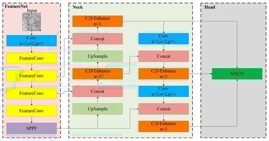
Figure 1.
FEM-YOLO network structure.
- (1)
- A lightweight FeatureNet network is adopted as the backbone network for feature extraction. Through more efficient parameter sharing and feature extraction mechanisms, the complexity of the model is reduced.
- (2)
- The C2f-Enhance module is designed, which combines the integration of EnhanceConv and C2f modules. This improves the representation capability of details and edges in feature maps, enhances detection accuracy, and does not increase the number of model parameters or computational load.
- (3)
- To further improve detection accuracy while achieving lightweight design, a lightweight shared convolution detection head (MSCD) is developed. By sharing weight parameters, the overall number of parameters is reduced.
- (4)
- The adopted Focal_EIoU loss function combines the advantages of Focal-Loss and EIoU. It enhances the algorithm performance when processing challenging samples and simultaneously penalizes deviations in position and shape, improving localization accuracy.
2. Materials and Methods
2.1. Baseline Network
YOLOv8n is an end-to-end anchor-free general object detection network built on the basis of YOLOv5. This algorithm integrates the advantages of other advanced algorithms and introduces new features and improvements to further enhance performance and flexibility [19]. YOLOv8n has transformed from a coupled head architecture to a decoupled head architecture, and adopts an anchor-free design to avoid hyperparameter issues associated with anchor boxes. The convolution kernel size of its first convolutional layer is reduced from 6 × 6 to 3 × 3, thereby decreasing the number of parameters. In addition, the C2f module replaces the C3 module, providing more skip connections and additional split operations.
However, the features of steel strip surface defects have almost no obvious visual distinction from the background; the captured images usually have low resolution, and the defects are small, dense, and unevenly distributed. Therefore, due to the lack of contextual information, YOLOv8n may face difficulties in detecting these defects, which may lead to a significant impact of negative samples on detection and result in discontinuities. Furthermore, the baseline algorithm YOLOv8n has high computational requirements and high algorithm complexity. Due to the limitation of the computing capacity of terminal devices, its application in the field of steel strip surface defect detection is restricted.
The network architecture of the FEM-YOLO algorithm proposed in this paper is shown in Figure 1. Its backbone network is designed as FeatureNet, which significantly saves computing resources and reduces the number of parameters. Moreover, the designed EnhanceConv is integrated into the C2f module, which further saves computing resources and reduces the number of parameters. In addition, a lightweight shared convolution detection head (MSCD) is designed in the algorithm head. By minimizing the number of parameters and computational load, it improves the operation speed while maintaining high detection accuracy.
2.2. FEM-YOLO Structure
2.2.1. FeatureNet Network
CSPDarkNet53 serves as the backbone network of YOLOv8. Although it reduces the computational burden by leveraging the CSP (Cross-Stage Partial) structure, it still belongs to a relatively heavyweight model, resulting in slow inference speed when processing high-resolution images. Despite the design of cross-stage feature propagation, its feature reuse mechanism is not as efficient as that of modern networks; the connection of some convolution blocks is relatively simple, which may lead to insufficient feature extraction capability in complex scenarios. In addition, CSPDarkNet53 exhibits poor flexibility in terms of task adaptability and diversified applications, especially when dealing with targets of extreme sizes, its performance is limited. To address these issues, this paper proposes FeatureNet to replace the backbone network CSPDarkNet53. FeatureNet adopts a four-layer hierarchical architecture, as shown in Figure 2, integrating convolutional downsampling and modified FeatureConv for feature extraction. To improve efficiency, Batch Normalization is used instead of Layer Normalization, and it is placed after depthwise separable convolution to support fusion during inference. Inspired by MobileNeXt, FeatureNet adds depthwise separable convolution at the end of each block, sets the channel expansion factor to 4, and doubles the network width at each stage. Furthermore, the GELU activation function in FeatureConv is replaced with ReLU6, which further enhances the model’s efficiency.
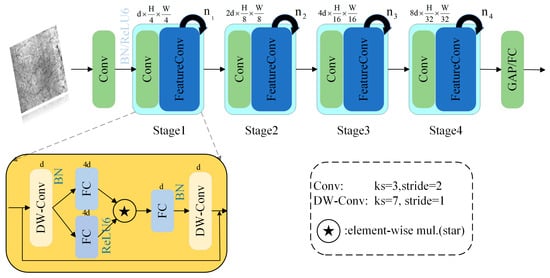
Figure 2.
Structure of FeatureNet and FeatureConv.
Among them, the Depthwise Separable Convolution Module (DW-Conv) is an improvement over traditional convolution. By decoupling the correlations between the spatial dimension and the channel dimension, it reduces the number of parameters required for convolution computation. As shown in Figure 3, the DW-Conv computation mainly consists of two parts: the first part is Depthwise Convolution. Different from the traditional convolution process, Depthwise Convolution separates channels, and the number of convolution kernels is the same as the number of channels of the input feature map; each convolution kernel has 1 channel, and one convolution kernel only operates on one input channel. Finally, the number of channels of the generated feature map is the same as that of the input. The second part is Pointwise Convolution, which mainly has two functions: first, freely setting the size of the output channel number, where the output channel number is equal to the number of 1D convolution kernels in Pointwise Convolution; second, fusing inter-channel information. Since Depthwise Convolution ignores inter-channel information, 1D convolution can be used to fuse such information.
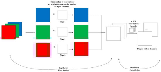
Figure 3.
Structure of DW-Conv. (“*” denotes convolution operation).
FeatureNet leverages the Element Wise Transform (EWT) to innovate the mapping of inputs into a high-dimensional, non-linear feature space without the need for expanding the network architecture. EWT provides high performance, low latency, and relatively low energy consumption, all within a compact network structure. By utilizing EWT, FeatureNet can map features into a high-dimensional and non-linear space without increasing computational complexity. The detailed mathematical derivation of EWT is presented in “Appendix A”.
The design of EWT consists of four key steps: (1) Select input features, which can be derived from any layer of the network; (2) Perform element-wise multiplication; (3) Map the features to a high-dimensional space; (4) Integrate the transformed features back into the network, allowing the features to be mapped to a higher dimension through EWT. This process expands the feature space dimension layer by layer using element-wise multiplication, without adding significant computational burden. Multi-layer EWT enables recursive increases in the implicit feature dimension, ultimately enhancing the network’s ability to process complex features.
For YOLO-based networks, the Element Wise Transform (EWT) significantly enhances the expressiveness of feature representations, making it particularly effective for tasks like steel strip defect detection. FeatureNet leverages multi-layer EWT to improve the quality of feature extraction, thereby boosting detection accuracy. Unlike traditional lightweight backbones that primarily focus on reducing computation, FeatureNet takes a different approach by fundamentally enhancing the non-linear feature representation capacity. Through EWT, it enables high-dimensional feature mapping without the need for architectural expansion. This innovative mechanism strikes a novel balance between richer feature representations and computational efficiency, avoiding the complexity and overhead typically associated with more intricate network designs.
2.2.2. C2f-Enhance Module
The C2f module is based on the CSPNet (Cross-Stage Partial Network) architecture. It reduces parameters and computational complexity by sharing partial weights, and aggregates cross-stage features using skip connections to improve detection performance. However, the C2f module also has some limitations:
First, multiple independent convolutional layers may lead to parameter redundancy in deep networks, especially for similar or redundant weights.
Second, since features are split into two branches—particularly when multiple convolutional layers are used in the main branch—the computational overhead increases, reducing computational efficiency. This issue is more prominent when processing large inputs or high-resolution images.
Finally, the feature fusion of C2f is implemented through simple concatenation operations, which fail to fully utilize multi-scale features and may thus affect performance.
To address the aforementioned issues, this paper proposes the C2f-Enhance module, as shown in Figure 4. Inspired by the DEA-Net (Image Dehazing Network) proposed in Reference [30], the C2f module is improved by introducing Enhanced Convolution (EnhanceConv) to replace traditional convolution, thereby enhancing the edge information extraction capability and reducing parameter complexity. The C2f-Enhance module splits the input features into two parts: one part is directly output through a skip connection, and the other part undergoes the EnhanceConv operation. EnhanceConv combines traditional convolution and Difference Convolution to enhance high-frequency information (such as edges and contours), which is conducive to more accurate defect identification.
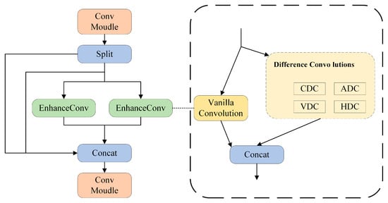
Figure 4.
Structure of C2f-Enhance with EnhanceConv.
Difference Convolution includes the following types:
Central Difference Convolution (Central DC): It captures edges in vertical and horizontal directions, and is suitable for detecting micro-cracks or pits.
Angular Difference Convolution (Angular DC): It captures edges in different directions, helping to detect oblique defects.
Horizontal Difference Convolution (Horizontal DC): It detects horizontal scratches.
Vertical Difference Convolution (Vertical DC): It detects vertical cracks.
These types of Difference Convolution enhance the gradient information of images and improve the capability to capture defect details. To reduce computational overhead, this paper simplifies multiple parallel convolutions into a single standard convolution by leveraging the additivity of convolutional layers while maintaining the same output effect. Given the input feature (Fin), EnhanceConv can utilize reparameterization technology to output (Fout) to a normal convolutional layer with the same computational cost and inference time. The formula is as follows (biases are omitted for simplification):
Among them, EnhanceConv() denotes the EnhanceConv convolution operation proposed in this paper. Ki, where i = 1–5, respectively, represent the kernels of VC (Vertical Convolution), CDC (Central Difference Convolution), ADC (Angular Difference Convolution), HDC (Horizontal Difference Convolution), and VDC (Vertical Difference Convolution), denotes the convolution operation; and Kcvt denotes the converted kernel, which merges the parallel convolutions together. The process of the reparameterization technology is shown in Figure 5.
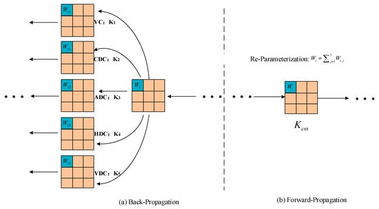
Figure 5.
Reparameterization technique process. (The “⋯” in the figure denotes the omitted convolution steps).
In the backpropagation phase, the kernel weights of the five parallel convolutions are updated separately through the chain rule of gradient propagation. In the forward propagation phase, the kernel weights of the five parallel convolutions remain fixed, and the weight of the converted kernel (Kcvt) is calculated by summing these weights at their corresponding positions. It is worth noting that the reparameterization technology can accelerate both the training and testing processes, as both processes include the forward propagation phase.
The reparameterization technique effectively reduces both computational and memory overhead by merging five parallel convolutions—one traditional convolution and four types of Difference Convolutions—into an equivalent convolution operation. During the training phase, EnhanceConv updates the weights of each of the five convolution kernels separately. However, during the forward propagation phase, these weights are accumulated to form a unified equivalent convolution kernel. This approach retains the advantages of parallel convolutions for feature extraction while significantly reducing computational and memory costs. Traditional convolutions capture intensity-level information, while Difference Convolutions emphasize gradient-level information. The combination of both enhances the feature extraction capability, making it especially effective for steel strip surface defect detection. In addition to reducing parameters, the C2f-Enhance module introduces a new feature representation dimension—the gradient space—by leveraging multi-directional Difference Convolutions. When combined with reparameterization, this creates a structure-folding mechanism that preserves the benefits of multi-path learning while maintaining the efficiency of single-path inference. This novel approach strikes a balance between feature richness and computational efficiency, making it ideal for tasks that demand both high accuracy and fast processing.
2.2.3. Multi-Path Shared Convolution Detector Head
In steel plate surface defect detection, this detection task faces numerous challenges due to the irregular shapes of defects and significant variations in their heights. YOLOv8 adopts an advanced decoupled head structure: by separating the classification and detection branches independently, each branch consists of two 3 × 3 convolutional layers and one 1 × 1 convolutional layer, which significantly improves detection performance. However, this design also leads to a substantial increase in the number of parameters, which may affect the overall efficiency of the algorithm in environments with limited computing resources. Meanwhile, since each detection head of YOLOv8 receives inputs from different feature maps separately, there is a lack of effective information interaction between the detection heads. This may result in feature loss, thereby affecting the detection effect.
To address the aforementioned issues, this paper proposes MSCD, which aims to improve the algorithm’s operating efficiency by reducing the number of parameters and computational overhead while maintaining high detection accuracy. The structural design of MSCD is shown in Figure 6. After the feature extraction network outputs three feature layers, each branch first performs channel adjustment through a 1 × 1 convolutional layer, unifying the number of channels of the three input feature layers to the intermediate channel number A. Subsequently, all feature layers are integrated into a shared convolution module for feature extraction, and 3 × 3 convolution kernels are adopted to reduce parameter and computational requirements. In the final branch, the regression and classification tasks are processed independently: the regression branch predicts the bounding box coordinate offsets through a 1 × 1 convolutional layer, and to address the localization problem caused by target scale differences among different detection heads, a scale adjustment layer is introduced to adapt to defects of different sizes. The classification branch predicts the probability of each category through a 1 × 1 convolutional layer. It is worth noting that the weights of the convolutional layers in the regression and classification branches are independent, which enables the algorithm to optimize the localization and classification tasks separately.
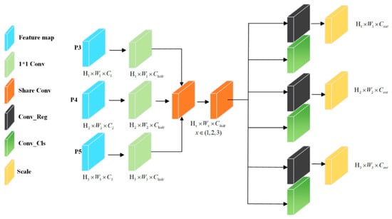
Figure 6.
MSCD network structure.
In summary, the MSCD head introduces a multi-scale shared learning mechanism that enables efficient information exchange between detection heads. By combining a shared feature space with task-specific branches, MSCD achieves collaborative optimization of localization and classification while maintaining the compactness of the overall structure.
2.2.4. Focal_EIoU Loss Function
Object detection typically uses Intersection over Union (IoU)-based loss functions to evaluate the overlap between predicted bounding boxes and ground-truth bounding boxes. However, IoU has limitations in addressing issues of inaccurate localization and inconsistent shapes. To this end, extended versions such as Generalized IoU (GIoU) and Distance IoU (DIoU) have been proposed. This paper proposes a new loss function, Focal-EIoU, which combines Focal Loss and Weighted IoU (WIoU) to replace CIoU in the baseline network. Focal-EIoU effectively solves the problems of class imbalance and localization accuracy.
Efficient IoU (EIoU): This method improves the calculation of IoU on the basis of IoU by introducing penalties for the width and height differences between the predicted box and the ground-truth box. The calculation formula of EIoU loss is as follows:
In this context, denotes the squared distance between the centers of the two bounding boxes, denotes the squared diagonal distance of the minimum enclosing box, and correspond to the differences in width and height, respectively, and represent the squared sizes of the bounding boxes.
Focal Loss was originally proposed to address the class imbalance problem in classification tasks. It reduces the weight of easily classifiable samples, thereby focusing more on hard-to-classify samples. The standard formula of Focal Loss is as follows:
In this context, denotes the probability of predicting the correct category, is the balancing factor, and is the parameter that controls the focus, which is used to adjust the degree of down-weighting for easily classifiable samples.
In the context of bounding box regression, the concept of Focal Loss is applied to penalize poor prediction performance, especially by weighting lower Intersection over Union (IoU) values—particularly when the overlap between the predicted bounding box and the ground-truth bounding box is insufficient. This is particularly important in object detection, as algorithms often predict low-quality bounding boxes. The Focal-EIoU loss function combines the principles of Focal Loss and EIoU (Efficient IoU), aiming to solve the localization problem and focus on objects that are difficult to localize. The formula of the Focal-EIoU loss function is as follows:
The expression of the focus weight is as follows:
The focus weight in this part dynamically adjusts the contribution of each bounding box based on the IoU value. Lower IoU values are assigned higher weights, encouraging the algorithm to focus more on challenging samples (i.e., bounding boxes with inaccurate localization). Parameters and control the strength of this down-weighting. In practical applications, is usually set between 0.5 and 2.0, while α is used to balance the contributions of easily classifiable samples and hard-to-classify samples. The EIoU component, which is the second part of the formula, is based on IoU and further penalizes the distance between the predicted center and the ground-truth center, as well as the width and height differences between the predicted box and the ground-truth box. This component helps improve regression accuracy, especially when there are significant differences in the shapes of bounding boxes.
The final Focal-EIoU loss function combines the advantages of Focal Loss and EIoU, enabling the algorithm to prioritize focusing on samples that are difficult to localize while improving detection accuracy by penalizing inconsistencies in localization and shape. The Focal-EIoU loss function introduces two penalty terms:
Distance Penalty: This term reflects the center point offset between and , where is the Euclidean distance between the center points, and is the diagonal length of the minimum enclosing box: .
Shape Penalty: This term penalizes the width and height differences between bounding boxes: ,
The combined Focal-EIoU loss formula can be expressed as:
The Focal-EIoU loss function effectively addresses two key issues in object detection: class imbalance and localization accuracy. By combining the advantages of Focal Loss and EIoU (Efficient IoU), this loss function not only improves the algorithm’s performance on challenging samples but also enhances localization accuracy through penalties for position and shape deviations. Therefore, Focal-EIoU is particularly suitable for complex object detection scenarios that require accurate localization and handling of shape variations.
3. Results
3.1. Dataset
This paper uses the public steel strip surface defect dataset from Northeastern University (NEU-DET), as shown in Figure 7. This dataset contains six types of defects: Cracks (Cr), Inclusions (In), Patches (Pa), Pitted Surfaces (Ps), Rolled-in Scale (Rs), and Scratches (Sc).Each defect type has 300 images, totaling 1800 images, which are augmented to 3600 images through random transformations. The dataset is divided into a training set, validation set, and test set in an 8:1:1 ratio, with 2880, 360, and 360 images, respectively. The defect types exhibit different sizes, shapes, texture features, and uneven distributions. In particular, the images of Cr and Rs defects face problems of irrelevant noise and uneven distribution, while Ps, Pa, and Sc defects have low contrast issues. These factors can affect detection performance, leading to missed detections and reduced algorithm feasibility.
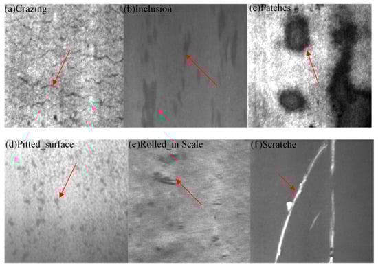
Figure 7.
Sample of surface defects on strip steel. (a) Cr. (b) In. (c) Pa. (d) Ps. (e) Rs. (f) Sc.
3.2. Experimental Setup
During the training phase, this study utilized four GPUs (NVIDIA TITAN XP) and employed Python 3.8 as the programming language, with PyTorch 2.1.0 as the deep learning library and PyCharm 2023 as the integrated development environment. The experimental parameters are summarized in Table 1. The input image size was set to 640 × 640, and data augmentation was performed using the Mosaic method. The initial learning rate was set to 0.01, with a cosine annealing strategy used to adjust the learning rate throughout training. The batch size was configured to 16, and the SGD optimizer was selected. Dropout regularization was applied, and the training was conducted over 300 epochs. Unless otherwise stated, all experiments in this study were performed using the above settings.

Table 1.
The experimental setup.
3.3. Dataset Augmentation Methods
In steel strip defect detection, the performance of deep learning models heavily depends on a large and diverse training dataset. However, image data for steel strip defects is often limited, with insufficient samples to cover all possible defect scenarios. This scarcity of data restricts the model’s generalization ability, making it challenging to maintain effective detection performance, especially when dealing with complex or previously unseen defects. To address this challenge, employing data augmentation techniques to generate diverse training data has become a crucial strategy. This paper introduces a data augmentation method based on random image transformations to improve the robustness and generalization ability of the steel strip defect detection model. The method involves randomly applying several image transformation operations to generate augmented samples that differ from the original images while preserving the core defect information. These transformations include horizontal flipping, random rotation, scaling, translation, and random adjustments to brightness and contrast. Although generative models and similar methods also offer advantages, random transformations are a suitable choice for processing steel defect detection data due to their simplicity and efficiency. They can quickly increase the diversity of the data without introducing excessive computational overhead, making them especially well-suited for real-time applications. By applying these transformations, the diversity of the training data is significantly increased, allowing the model to better adapt to a wide range of steel strip defects.
(1) Horizontal Flipping.
Images are randomly flipped horizontally with a 50% probability. This operation generates symmetrical samples, simulating variations in defect orientation that may arise during the actual production process.
(2) Random Rotation and Scaling.
Images are randomly rotated between 0 and 90 degrees and scaled within a 50% range, with a 50% probability. This simulates variations in the angle and size of defects, enabling the model to detect defects at different scales and orientations.
(3) Translation Transformation.
The images are translated with a displacement ratio limited to 0.1. This transformation enhances the model’s robustness to changes in defect location.
(4) Brightness and Contrast Adjustment.
The brightness and contrast of images are randomly adjusted with a 20% probability. This color transformation helps the model maintain sensitivity to defects under varying lighting conditions, improving its adaptability in real-world industrial environments.
The Albumentations library is employed to implement these augmentation operations, with all transformations tailored to the practical scenarios of steel strip defects, ensuring that the transformed images retain the essential characteristics of the defects. Through this data augmentation approach, the extended dataset significantly enhances the performance of the model. Augmented data are generated using defects such as Inclusions (In) and Rolled-in Scale (Rs) as examples, as shown in Figure 8.
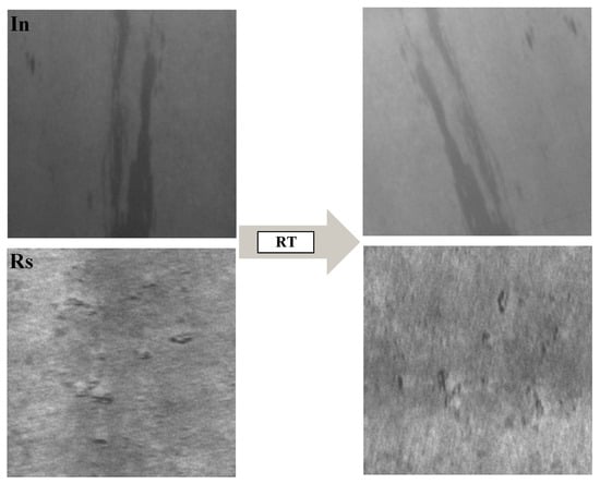
Figure 8.
Enhanced dataset.
3.4. Evaluation Metrics
This paper uses four metrics to evaluate the performance of the algorithm: mAP (mean Average Precision), FPS (Frames Per Second), algorithm parameter count (Params), and computational complexity (GFLOPs). mAP represents the average precision of all detected objects on the test set; a higher mAP value indicates better detection performance of the algorithm on objects of different categories. FPS measures the number of images processed by the algorithm per unit time; a higher FPS value means stronger real-time performance of the algorithm. The parameter count (Params) evaluates the complexity of the algorithm, and a smaller parameter count indicates that the algorithm is more lightweight. The GFLOPs metric evaluates the computational efficiency of the algorithm; a lower GFLOPs value indicates higher computational efficiency of the algorithm.
3.5. Comparative Experiments
3.5.1. Comparison of Different IoU Loss Functions
To verify the effectiveness of the proposed Focal_EIoU loss function, this paper compares the algorithm with the default CIoU of the baseline network and other loss functions (including EIoU, GIoU, and DIoU). The comparison results are shown in Table 2, which presents the classification performance of different loss functions for six types of steel strip surface defects. Focal_EIoU exhibits relatively balanced performance, with an mAP of 83.3%. The default CIoU of the baseline network performs poorly in detecting Cr and Rs defects, with mAP values of only 63.9% and 68.9%, respectively, and also shows unsatisfactory performance in detecting other defects. GIoU achieves an mAP of 84.1% in detecting In defects but has low detection rates for Cr and Sc, which are 57.3% and 94.7%, respectively, indicating that GIoU fails to provide balanced detection across different defect types. DIoU shows a significant improvement in detecting Ps defects, with an mAP of 87.6%, and performs best in detecting Pa defects, reaching 90.4%. However, it does not solve the problem of detecting Cr and Rs defects and fails to provide balanced performance across all defect categories. The network using Focal_EIoU in this paper achieves the best overall performance.
Table 2.
Comparison of different IoUs on NEU-DET dataset.
With an mAP of 83.3%, it effectively addresses the shortcomings of CIoU in Cr and Rs defect detection while maintaining relatively balanced performance for other defects. The mAP decline when using SIoU may be related to its design, as it focuses more on standardized object detection. In contrast, steel strip defects typically exhibit characteristics of being small and slender and having diverse morphological variations. In this case, the geometric constraint mechanism of SIoU may have insufficient sensitivity to small objects, resulting in inadequate localization and recognition capabilities for tiny defects. The Focal_EIoU loss function adopted in this paper combines the advantages of Focal Loss and EIoU, enhancing the algorithm’s performance when dealing with challenging samples while penalizing deviations in position and shape to improve localization accuracy. Therefore, Focal_EIoU is suitable for the scenario of steel strip surface defect detection.
Through comparative experiments with various loss functions, we observed that the recognition accuracy for Cr defects is significantly lower than the average accuracy for the other five defect types. This issue poses a major challenge in steel strip defect detection. The visual features of Cr defects are less distinct compared to those of other defect categories, which may hinder the model’s ability to effectively distinguish Cr defects from the background or other normal areas, leading to decreased recognition accuracy. Furthermore, under experimental conditions involving specific noise, background interference, or uneven lighting, the detection of Cr defects becomes even more difficult. We attempted to enhance the representation of Cr defects, but this led to a new issue of class imbalance, where the proportion of Cr defects in the training data became disproportionately large. This, in turn, degraded the model’s ability to recognize other defect categories. Future work on Cr defect detection should focus on targeted algorithm improvements, such as incorporating domain-specific knowledge related to defects, implementing multi-scale analysis, or employing advanced data augmentation techniques, in order to further improve the model’s ability to detect these challenging cases.
3.5.2. Comparison of Different Defect Detection Algorithms
The proposed FEM-YOLO algorithm in this paper demonstrates the best performance in terms of mAP, algorithm parameter count, computational load, and FPS for steel strip surface defect detection. Compared with the baseline YOLOv8, FEM-YOLO increases the mAP by 8.4%, reduces the algorithm parameter count by 1.8 M, and decreases the computational load from 8.7 GFLOPs to 4.6 GFLOPs (a reduction of 4.1 GFLOPs). The results of comparative experiments with other State-of-the-Art (SOTA) algorithms are shown in Table 3. FEM-YOLO significantly outperforms FastRCNN and SSD in terms of mAP, algorithm parameter count, and computational load. In the FPS performance test, FEM-YOLO also outperforms FastRCNN, SSD, YOLOv3, YOLOv5, YOLOv9, YOLOv10, and YOLOv11. Although the FPS performance of FEM-YOLO is slightly lower than that of YOLOv6 and YOLOv8, it still exhibits superior performance over YOLOv6 and YOLOv8 in terms of mAP, algorithm parameter count, and computational load.
Although YOLOv3 achieves an mAP of 79.9%, its algorithm parameter count and computational load are much higher than those of other YOLO series networks, thus failing to meet the lightweight standards. Furthermore, compared with the latest YOLOv11, FEM-YOLO shows better performance in model accuracy, parameter count, and computational volume. Table 3 also presents the results of comparative experiments with algorithms proposed in references [11,23,30,31,32,33,34]—all of which are the latest steel strip surface defect detection algorithms developed in the past two years. These algorithms are all applied to steel strip surface defect detection and use the NEU-DET dataset. Due to the fact that some references do not specify the hardware used, FPS comparison was not conducted. The DCAM-Net algorithm [11] has an mAP of 82.6% and a parameter count of 31.0 M. The YOLOv8-VSC algorithm [23] has an mAP of 80.8%, a parameter count of 1.96 M, and a computational cost of 6.0 G. The LF-YOLO algorithm [31] has an mAP of 83.7% and a computational cost of 88.7 G. The MCB-FAH-YOLOv8 algorithm [32] has an mAP of 81.8% and a parameter count of 6.06 M. The improved YOLOv8 algorithm [33] has an mAP of 81.1%, a parameter count of 4.9 M, and a computational volume of 9.2 G. The EHH-YOLOv8s algorithm [34] has an mAP of 79.7%, a parameter count of 7.0 M, and a computational cost of 15.6 G. Although the mAP of the LF-YOLO algorithm is 0.4% higher than that of FEM-YOLO, its computational cost is 88.7 G, which is much higher than the 4.6 G of FEM-YOLO. The FEM-YOLO algorithm designed in this paper is more lightweight compared with other steel strip defect detection algorithms. In summary, the proposed FEM-YOLO has the advantages of small algorithm size and low computational load while ensuring detection accuracy.
In summary, compared to algorithms such as YOLOv8-VSC, the proposed method not only excels in parameter compression but also significantly improves recognition accuracy while maintaining high computational speed. The introduced FeatureNet, C2f-Enhance, and MSCD modules bring fundamental innovations across three levels. FeatureNet expands the representation dimension through non-linear high-dimensional mapping (EWT), redefining the balance between efficiency and expressiveness. C2f-Enhance extends the feature domain from intensity space to gradient space, enhancing the perception of defect details. MSCD restructures the information flow through shared multi-scale convolutions, enabling minimal redundancy and inter-head collaboration. Together, these mechanisms establish a unified design philosophy that emphasizes representation richness, structural efficiency, and inter-module collaboration.
Table 3.
Comparison of different strip steel detection algorithms on NEU-DET dataset.
Table 3.
Comparison of different strip steel detection algorithms on NEU-DET dataset.
| Model | mAP (%) | Param (M) | FLOPs (G) | FPS |
|---|---|---|---|---|
| FastRCNN | 75.9 | 137.1 | 370.2 | 10 |
| SSD | 73.2 | 26.3 | 62.7 | 22 |
| YOLOv3 | 79.9 | 61.5 | 105 | 25 |
| YOLOv5 | 73.5 | 2.5 | 7.2 | 213 |
| YOLOv6 | 74.3 | 4.2 | 11.9 | 293 |
| YOLOv8 | 74.9 | 3.2 | 8.7 | 302 |
| YOLOv9 | 78.8 | 7.2 | 26.7 | 88.7 |
| YOLOv10 | 71.9 | 2.3 | 6.7 | 231 |
| YOLOv11 | 80.9 | 2.6 | 6.6 | 242 |
| [30] | 83.7 | - | 88.7 | - |
| [23] | 80.8 | 1.96 | 6.0 | - |
| [32] | 81.8 | 6.06 | - | - |
| [11] | 82.6 | 31.0 | - | - |
| [33] | 81.1 | 4.9 | 9.2 | - |
| [34] | 79.7 | 7.0 | 15.6 | |
| Ours | 83.3 | 1.4 | 4.6 | 265 |
Note: Bolded data represents the best-performing data, while underlined data represents the second-best.
3.5.3. Visual Comparison Experiment of Steel Strip Surface Defect Detection
In this paper, visual comparison experiments were conducted using the optimal weights of the trained YOLO series steel strip defect detection algorithms, and the results are shown in Figure 9. In the figure, the blue, white, dark blue, cyan, light blue, and purple boxes represent the detection results of Cr, Pa, Rs, Ps, In, and Sc, respectively. The detection results show that YOLOv3, YOLOv5, YOLOv6, YOLOv8, YOLOv9, and YOLOv10 all perform well in detecting Pa, Rs, In, and Sc defects. However, except for the method proposed in this paper, other methods fail to completely detect Cr defects or have low confidence in detection results. This problem stems from the low contrast in surface defect images—Cr exhibits complex texture features and significant irrelevant noise, making it difficult for the detection network to accurately capture its position, which in turn leads to missed detections. FEM-YOLO effectively improves the detection capability for such defects, enabling more accurate capture of key features in images with rich details, thereby enhancing the accuracy of object detection and better capturing Cr defects. In addition, when detecting Ps defects, networks such as YOLOv5, YOLOv6, YOLOv8, YOLOv9, and YOLOv10 face difficulties in accurately localizing defects, resulting in defect merging or missed detections. This limitation is attributed to the insufficient overall feature extraction capability of these networks when dealing with irregular defects. The FEM-YOLO algorithm proposed in this paper enhances the correlation between the target features of irregular steel strip defects, enabling the detection network to obtain more comprehensive defect feature information and improving the feature extraction capability.
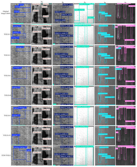
Figure 9.
Visualization results of different algorithms for detection of six defects in strip steel.
3.6. Ablation Experiments
To validate the effectiveness of FEM-YOLO, YOLOv8n was adopted as the baseline network, and progressive performance evaluations were conducted for each improvement, including data augmentation, replacement of the backbone with FeatureNet, incorporation of the improved C2f-Enhance module, and integration of the Multi-path Shared Convolutional Detection (MCSD) module. The results of the ablation experiments for each enhancement module are presented in Table 4. As shown in Table 4, the first enhancement involves data augmentation. The application of a Random Transformation (RT) method improves the feature representation of the augmented defect images, enabling the algorithm to learn defect characteristics more effectively. Consequently, the mean Average Precision (mAP) increased from 74.9% (baseline YOLOv8n) to 77.2%. Building upon this, FeatureNet was introduced to replace CSPDarkNet as the backbone network. With the use of FeatureConv, richer and more expressive feature representations were obtained without requiring complex network designs or additional computational costs. This modification made the overall network more compact and efficient—the floating-point operations (FLOPs) decreased from 8.7 G to 6.5 G, the number of parameters was reduced by 1 M, and the FPS increased by 16. Furthermore, the improved C2f-Enhance module, equipped with EnhanceConv, enhanced the algorithm’s average precision by 1.5%. However, a decrease in FPS from 318 to 278 was observed. This reduction is attributed to the increased computational time required by the C2f-Enhance module, which strengthens the model’s feature extraction capability and improves detection accuracy and feature expressiveness. Despite the decline in FPS, this precision improvement provides a significant advantage in practical steel defect detection scenarios. Finally, the designed Multi-path Shared Convolutional Detection (MCSD) head further reduced the model size, lowering the FLOPs to 4.6 G and the number of parameters to 1.4 M while increasing the mAP to 79.2%.
Table 4.
FEM-YOLO algorithm ablation experiments.
The results of the ablation experiments clearly indicate that the improved FEM-YOLO algorithm outperforms the YOLOv8n algorithm. Specifically, FEM-YOLO achieves a 4.2% improvement in mAP while reducing both the computational load and parameter count to 43.7% and 52.9% of the baseline algorithm, respectively, with only a reduction of 37 FPS. Despite this decrease, FEM-YOLO maintains a high processing speed of approximately 256 FPS, without significantly compromising computational accuracy or requiring additional computational resources. In other words, our method successfully strikes a balance between high real-time throughput, accuracy, and efficient resource utilization. Overall, the performance of the FEM-YOLO algorithm surpasses that of YOLOv8n.
3.7. Algorithm Feasibility Verification
To further verify the feasibility of the proposed FEM-YOLO algorithm, this paper compares the performance of YOLOv8n and FEM-YOLO on the Aluminum Surface Defect Dataset (APSPC) and the GC10-DET dataset, respectively, so as to further illustrate the feasibility of the FEM-YOLO algorithm. The Aluminum Surface Defect Dataset (APSPC) contains 1885 aluminum surface defect images, divided into ten defect categories: Dents, Non-conductive Areas, Scratches, Orange Peel, Bottom Leaks, Impacts, Pits, Protruding Powder, Coating Cracks, and Stains. The GC10-DET dataset is a real-world surface defect dataset derived from industrial environments, including ten types of surface defects: Punching (Pu), Welding Seam (Ws), Crescent Gap (Cg), Water Stains (Ws), Oil Stains (Os), Silk Spots (Ss), Inclusions (In), Rolling Pits (Rp), Creases (Cr), and Waist Creases (Wf). All defects appear on the steel plate surface, and this dataset contains 3570 grayscale images. Both datasets are divided into a training set, validation set, and test set in an 8:1:1 ratio. The experimental setup is consistent with the above, and the experimental results are shown in Figure 10 and Figure 11.
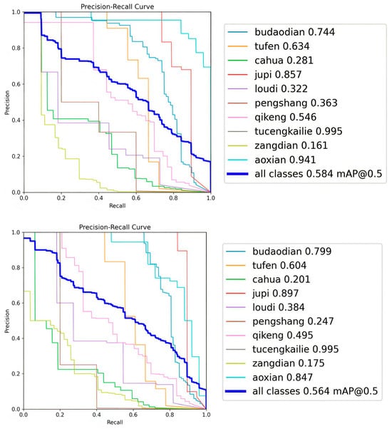
Figure 10.
Experimental results of the generalization study on the APSPC dataset.
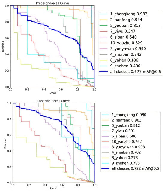
Figure 11.
Experimental results of the generalization study on the GC10-DET dataset.
3.7.1. Feasibility Study on the APSPC Dataset
The results obtained after training the YOLOv8n and FEM-YOLO models on the APSPC dataset are shown in Figure 10. The left figure is the PR (Precision-Recall) curve of the YOLOv8n model after training, and the right figure is the PR curve of the FEM-YOLO model after training. On the Aluminum Surface Defect Dataset (APSPC), the mAP of the baseline algorithm after training is 56.4%, while the mAP of the FEM-YOLO algorithm after training is 58.4%. Compared with the baseline algorithm, the proposed FEM-YOLO increases the mAP by 2%, which can prove that the FEM-YOLO algorithm has good feasibility.
3.7.2. Feasibility Study on the GC10-DET Dataset
The results obtained after training the baseline algorithm and the FEM-YOLO model on the GC10-DET dataset are shown in Figure 11. The left figure is the PR (Precision-Recall) curve of the YOLOv8n model after training, and the right figure is the PR curve of the FEM-YOLO model after training. On the GC10-DET dataset, the mAP of the baseline algorithm after training is 67.7%, while the mAP of the FEM-YOLO algorithm after training is 72.2%. Compared with the baseline algorithm, the proposed FEM-YOLO increases the mAP by 4.5%, which can prove that the FEM-YOLO algorithm has good feasibility.
Through the above two sets of experiments, it is indicated that the FEM-YOLO algorithm proposed in this paper is not limited to the NEU-DET dataset. Its good performance on the NEU-DET dataset is not accidental; it is also applicable to other datasets containing small defect types. Compared with YOLOv8n, it exhibits excellent performance and possesses certain feasibility.
3.8. Model Latency and System Energy Consumption
Model latency and system energy consumption are not only technical indicators but also key factors affecting user experience, operating costs, and system stability. Low latency ensures that user operations can receive timely feedback, improving user experience; low energy consumption means that the system consumes fewer hardware resources during operation, making it suitable for deployment on front-end devices with limited resources. By optimizing these two aspects, higher economic and social benefits can be achieved while improving system performance.
This paper uses model inference speed (Inference) as the evaluation criterion for model latency. The shorter the time required for inference speed, the better the latency performance of the model. As shown in Figure 12, this paper compares the inference speed of YOLOv3, YOLOv5, YOLOv6, YOLOv8, YOLOv9, YOLOv10, YOLOv11, and FEM-YOLO algorithms for a single steel strip scratch defect image, and their detection results are presented in the form of confidence. It can be found that YOLOv6 has the fastest inference speed of 147 ms, with the best model latency performance, but its confidence in predicting scratch defects is average at 0.47. After comprehensive comparison, it can be seen that the inference speed of FEM-YOLO is 158 ms, which is the fastest among algorithms except YOLOv6, and its confidence is also relatively high at 0.75. Compared with the baseline network YOLOv8, whose model inference speed is 160 ms, FEM-YOLO reduces the speed by 2 ms and increases the confidence by 0.35, which is sufficient to prove that the FEM-YOLO algorithm has relatively good model latency performance. For the comparison of system energy consumption, the lower the model’s parameter count (Params) and computational volume (GFLOPs), the easier it is to deploy to front-end hardware, the lower the requirement for hardware computing resources, and the lower the system energy consumption. The FEM-YOLO algorithm in this paper has a parameter count of 1.4 M and a computational volume of 4.6 G, both of which are lower than those of the compared deep learning object detection algorithms.
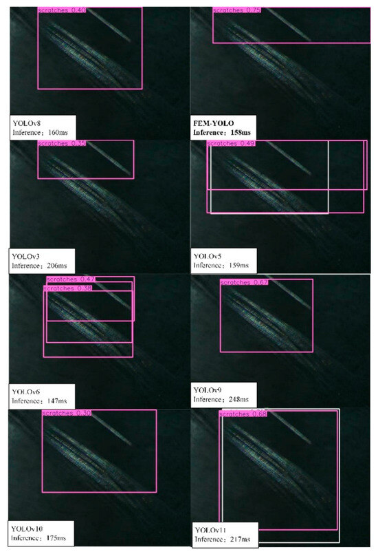
Figure 12.
Model inference speed comparison results.
3.9. Hardware Deployment Comparison Experiment
To validate that our model can adapt to lower computational resources, we conducted a comparative experiment by deploying FEM-YOLO and YOLOv8n on both the Jetson Nano and Jetson Nano NX. The results demonstrate that FEM-YOLO can maintain strong performance even with limited computational resources. As shown in Table 5, FEM-YOLO performs stably on the Jetson Nano, despite the hardware resource disparity compared to the Jetson Nano NX. Notably, there is minimal difference in recognition accuracy, power consumption, memory occupancy, and memory usage, all of which remain within acceptable limits. Additionally, it is worth mentioning that, under the same hardware resources, FEM-YOLO outperforms YOLOv8n in terms of overall performance.
Table 5.
Comparative Experiments of Different Algorithms on Various Hardware Deployments.
4. Conclusions
This study presents FEM-YOLO, a lightweight and efficient algorithm for detecting surface defects in steel strips. By utilizing the FeatureNet network for feature extraction and incorporating the C2f-Enhance module to enhance detail representation, FEM-YOLO improves detection accuracy without increasing computational costs. Additionally, the Multi-Path Shared Convolution Detection Head reduces the number of parameters while maintaining performance. The experimental results on the NEU-DET dataset demonstrate that FEM-YOLO achieves an mAP of 83.3% while reducing both the computational load and parameter count to 43.7% and 52.9% of the baseline algorithm, respectively, yielding significant improvements in efficiency and effectiveness. Future work will focus on addressing the challenges posed by defects such as steel strip surface cracks (Cr) and rolling scale (Rs), which are prone to background noise and may result in false positives or missed detections. Efforts will include further algorithm development, evaluation on more diverse datasets, and optimization for real-time applications in factory production lines, ensuring high accuracy while minimizing resource consumption.
Author Contributions
Conceptualization, Y.L.; Methodology, Y.Z.; Validation, Y.Z.; Investigation, Y.L.; Resources, Y.L.; Data curation, Y.L.; Writing—original draft, P.W.; Writing—review and editing, Y.Z.; Supervision, Y.Z.; Project administration, Y.L.; Funding acquisition, Y.L. All authors have read and agreed to the published version of the manuscript.
Funding
This research was funded by State Key Laboratory of Metal Forming Technology and Heavy Equipment grant number S2308100.W02. This research was funded by National Natural Science Foundation of China grant number Program No. 52307182. This research was funded by Doctoral Scientific Research Foundation of Xi’an Polytechnic University grant number Program No. BS202125.
Data Availability Statement
The data presented in this study are openly available in http://faculty.neu.edu.cn/songkechen/zh_CN/zdylm/263270/list/index.htm (accessed on 7 September 2025).
Conflicts of Interest
The authors declare no conflicts of interest.
Appendix A
- The mathematical derivation process of EWT.
In a single layer of the neural network, EWT is usually expressed as:
In the formula, the symbol “∗” denotes element-wise multiplication, which refers to the multiplication of corresponding elements of two matrices or vectors. For simplification, the weight matrices , as well as the bias matrices , are usually merged in to a single matrix , and the inputs are merged into a corresponding single matrix accordingly. In this way, EWT can be expressed as:
In this analysis, this paper simplifies the scenario by considering the transformation of a single output channel and single-element input. Specifically, this paper defines , , (where d denotes the input channel number). This can be easily extended to adapt to multiple output channels , , and process multiple feature elements, . EWT can be expanded through the following formula:
Among them, is the coefficient of each term, which is defined as:
Through this expansion, EWT involves dimensions. As increases, the size of this implicit dimensional space approaches . This characteristic is similar to the operation of kernel functions, which significantly increases the dimension of the feature space through efficient computation without introducing additional computational overhead.
Next, this paper proves that by stacking multiple layers, EWT can exponentially increase the implicit dimension during the recursive process, approaching an infinite dimension. Let the width of the initial layer be; after applying EWT, the obtained implicit feature space is expressed as:
If EWT is extended to multiple layers, assuming the output of the -th layer, then:
The implicit dimension of each layer increases as the number of layers increases. Specifically, the implicit feature space of the layer belongs to . For example, in a network with a width of 128 and 10 layers, after applying EWT, the implicit feature dimension is approximately 90 × 1024 × 90 × 1024, which can be reasonably approximated as an “infinite dimension”. By stacking multiple layers, EWT can significantly increase the implicit dimension even with only a small increase in the number of layers, and the growth follows an exponential trend. This process demonstrates how neural networks map to a high-dimensional space through layer stacking.
- 2.
- The FEM-YOLO algorithm and dataset are presented at https://github.com/uglly/TinyDefectNet.git (accessed on 7 September 2025).
- (1)
- The coupling teaching scheme of FEM-YOLO is introduced below. The following YAML file of FEM-YOLO clearly demonstrates its structural framework, where the module distribution is identical to the content presented in Figure 1. The input-output relationships between modules, as well as the convolution kernel sizes and strides, remain the same as in YOLOv8n.
| #FEM-YOLO backbone: |
| # [from, repeats, module, args] |
| - [−1, 1, FeatureNet, []] #4 |
| - [−1, 1, SPPF, [1024, 5]] #5 |
| # FEM-YOLO head |
| head: |
| - [−1, 1, nn.Upsample, [None, 2, "nearest"]] #6 |
| - [[−1, 3], 1, Concat, [1]] #7 cat backbone P4 |
| - [−1, 3, C2f_Ehance, [512]] # 8 |
| - [−1, 1, nn.Upsample, [None, 2, "nearest"]] #9 |
| - [[−1, 2], 1, Concat, [1]] #10 cat backbone P3 |
| - [−1, 3, C2f_Ehance, [256]] # 11(P3/8-small) |
| - [−1, 1, Conv, [256, 3, 2]] #12 |
| - [[−1, 8], 1, Concat, [1]] #13 cat head P4 |
| - [−1, 3, C2f_Ehance, [512]] # 14(P4/16-medium) |
| - [−1, 1, Conv, [512, 3, 2]] #15 |
| - [[−1, 5], 1, Concat, [1]] #16 cat head P5 |
| - [−1, 3, C2f_Ehance, [512]] # 17(P5/32-large) |
| - [[11, 14, 17], 1, Detect_MSCD, [nc,256]] # Detect (P3, P4, P5) |
- (2)
- Firstly, the backbone of YOLOv8 is replaced from CSPDarkNet53 to FeatureNet, consisting of four layers of FeatureNet. The main code for FeatureNet is as follows:
| class FeatureNet(nn.Module): |
| def __init__(self, base_dim = 32, depths = [3, 3, 12, 5], mlp_ratio = 4, drop_path_rate = 0.0, num_classes = 1000, **kwargs): super().__init__() |
| self.num_classes = num_classes |
| self.in_channel = 32 |
| # stem layer |
| self.stem = nn.Sequential(ConvBN(3, self.in_channel, kernel_size = 3, stride = 2, padding = 1), nn.ReLU6()) |
| dpr = [x.item() for x in torch.linspace(0, drop_path_rate, sum(depths))] # stochastic depth |
| # build stages |
| self.stages = nn.ModuleList() |
| cur = 0 |
| for i_layer in range(len(depths)): |
| embed_dim = base_dim * 2 ** i_layer |
| down_sampler = ConvBN(self.in_channel, embed_dim, 3, 2, 1) |
| self.in_channel = embed_dim |
| blocks = [Block(self.in_channel, mlp_ratio, dpr[cur + i]) for i in range(depths[i_layer])] |
| cur += depths[i_layer] |
| self.stages.append(nn.Sequential(down_sampler, *blocks)) |
| self.channel = [i.size(1) for i in self.forward(torch.randn(1, 3, 640, 640))] |
| self.apply(self._init_weights) |
- (3)
- Secondly, in the head, EnhanceConv is integrated into the C2f module to form C2f_Enhance, strengthening the feature extraction capability. The design code for this module is as follows:
| class C2f_Enhance(C2f): |
| def __init__(self, c1, c2, n = 1, c3k = False, e = 0.5, g = 1, shortcut = True): |
| super().__init__(c1, c2, n, c2f, e, g, shortcut) |
| self.m = nn.ModuleList( |
| C2f_Enhance(self.c, self.c, 2, shortcut, g) if c3k else C2f_Enhance (self.c) |
| for _ in range(n) |
| ) |
- (4)
- Finally, the detection head uses MCSD, where the extracted features are integrated through multiple paths to reduce information loss. The design code for this module is as follows:
| class Detect_MCSD(nn.Module): |
| # Multi-path Shared Convolutional Detection Head |
| """YOLOv8 Detect head for detection models.""" |
| dynamic = False # force grid reconstruction |
| export = False # export mode |
| shape = None |
| anchors = torch.empty(0) # init |
| strides = torch.empty(0) # init |
| def __init__(self, nc = 80, hidc = 256, ch = ()): |
| """Initializes the YOLOv8 detection layer with specified number of classes and channels.""" |
| super().__init__() |
| self.nc = nc # number of classes |
| self.nl = len(ch) # number of detection layers |
| self.reg_max = 16 # DFL channels (ch[0] // 16 to scale 4/8/12/16/20 for n/s/m/l/x) |
| self.no = nc + self.reg_max * 4 # number of outputs per anchor |
| self.stride = torch.zeros(self.nl) # strides computed during build |
| self.conv = nn.ModuleList(nn.Sequential(Conv_GN(x, hidc, 3)) for x in ch) |
| self.share_conv = nn.Sequential( |
| Conv_GN(hidc, hidc, 3, g = hidc), |
| Conv_GN(hidc, hidc, 1) |
| ) |
| self.cv2 = nn.Conv2d(hidc, 4 * self.reg_max, 1) |
| self.cv3 = nn.Conv2d(hidc, self.nc, 1) |
| self.scale = nn.ModuleList(Scale(1.0) for x in ch) |
| self.dfl = DFL(self.reg_max) if self.reg_max > 1 else nn.Identity() |
References
- Chen, S.; Fu, T.; Song, J.; Wang, X.; Qi, M.; Hua, C.; Sun, J. A lightweight semi-supervised distillation framework for hard-to-detect surface defects in the steel industry. Expert Syst. Appl. 2026, 297, 129489. [Google Scholar] [CrossRef]
- Chen, S.; Jiang, S.; Wang, X.; Ye, K.; Sun, J.; Hua, C. A high-precision and real-time lightweight detection model for small defects in cold-rolled steel. J. Real-Time Image Proc. 2025, 22, 30. [Google Scholar] [CrossRef]
- Zheng, H.; Chen, X.; Cheng, H.; Du, Y.; Jiang, Z. MD-YOLO: Surface defect detector for industrial complex environments. Opt. Lasers Eng. 2024, 178, 108170. [Google Scholar] [CrossRef]
- Kaur, R.; Mittal, U.; Wadhawan, A.; Almogren, A.; Singla, J.; Bharany, S.; Hussen, S.; Rehman, A.U.; Al-Huqail, A.A. YOLO-LeafNet: A robust deep learning framework for multispecies plant disease detection with data augmentation. Sci. Rep. 2025, 15, 28513. [Google Scholar] [CrossRef] [PubMed]
- Chen, S.; Jiang, S.; Wang, X.; Sun, P.; Hua, C.; Sun, J. An efficient detector for detecting surface defects on cold-rolled steel strips. Eng. Appl. Artif. Intell. 2024, 138, 109325. [Google Scholar] [CrossRef]
- Fan, Z.; Lu, D.; Liu, M.; Liu, Z.; Dong, Q.; Zou, H.; Hao, H.; Su, Y. YOLO-PDGT: A lightweight and efficient algorithm for unripe pomegranate detection and counting. Measurement 2025, 254, 117852. [Google Scholar] [CrossRef]
- Zhong, H.; Xiao, L.; Wang, H.; Zhang, X.; Wan, C.; Hu, Y.; Wu, B. LiFSO-Net: A lightweight feature screening optimization network for complex-scale flat metal defect detection. Knowl.-Based Syst. 2024, 304, 112520. [Google Scholar] [CrossRef]
- Kou, X.; Liu, S.; Cheng, K.; Qian, Y. Development of a YOLO-V3 based model for detecting defects on steel strip surface. Measurement 2021, 182, 109454. [Google Scholar] [CrossRef]
- Cheng, X.; Yu, J. RetinaNet with difference channel attention and adaptively spatial feature fusion for steel surface defect detection. IEEE Trans. Instrum. Meas. 2021, 70, 2503911. [Google Scholar] [CrossRef]
- Li, Z.; Tian, X.; Liu, X.; Liu, Y.; Shi, X. A two-stage industrial defect detection framework based on improved-YOLOv5 and optimized inception-ResnetV2 models. Appl. Sci. 2022, 12, 834. [Google Scholar] [CrossRef]
- Chen, H.; Du, Y.; Fu, Y.; Zhu, J.; Zeng, H. DCAM-Net: A rapid detection network for strip steel surface defects based on deformable convolution and attention mechanism. IEEE Trans. Instrum. Meas. 2023, 72, 5005312. [Google Scholar] [CrossRef]
- Xing, J.; Jia, M. A convolutional neural network-based method for workpiece surface defect detection. Measurement 2021, 176, 109185. [Google Scholar] [CrossRef]
- Wang, H.; Li, Z.; Wang, H. Few-shot steel surface defect detection. IEEE Trans. Instrum. Meas. 2022, 71, 5003912. [Google Scholar] [CrossRef]
- Cai, J.; Bai, J.; Zhang, X.; Zhou, T.; Li, J.; Gao, S. Metal sheet surface defect detection based on improved Mask R-CNN. J. Chongqing Univ. Sci. Technol. (Nat. Sci. Ed.) 2023, 25, 110–116. [Google Scholar] [CrossRef]
- Zhang, Z.C. Lightweight Strip Steel Defect Detection Based on Improved YOLOv5. Comput. Syst. Appl. 2023, 32, 278–285. [Google Scholar]
- Qin, R.; Chen, N.; Huang, Y. EDDNet: An Efficient and Accurate Defect Detection Network for the Industrial Edge Environment. In Proceedings of the 2022 IEEE 22nd International Conference on Software Quality, Reliability and Security (QRS), Guangzhou, China, 5–9 December 2022; pp. 854–863. [Google Scholar]
- Xie, Z.; Yu, Y. Lightweight defect detection algorithm for steel strips based on improved YOLOv8. Sci. Technol. Ind. 2024, 24, 223–230. [Google Scholar]
- Zhou, S.; Zeng, Y.; Li, S.; Zhu, H.; Liu, X.; Zhang, X. Surface Defect Detection of Rolled Steel Based on Lightweight Model. Appl. Sci. 2022, 12, 8905. [Google Scholar] [CrossRef]
- Yang, L.; Huang, X.; Ren, Y.; Huang, Y. Steel Plate Surface Defect Detection Based on Dataset Enhancement and Lightweight Convolution Neural Network. Machines 2022, 10, 523. [Google Scholar] [CrossRef]
- Yan, X.; Yang, Y.; Tu, N. Steel surface defect detection based on improved SSD. Mod. Manuf. Eng. 2023, 112–120. [Google Scholar] [CrossRef]
- Lu, J.Z.; Zhang, C.Y.; Liu, S.P.; Ning, D.J. Lightweight DCN-YOLO for Strip Surface Defect Detection in Complex Environments. Comput. Eng. Appl. 2023, 59, 318–328. [Google Scholar] [CrossRef]
- Wang, J.; Xu, P.; Li, L.; Zhang, F. DAssd-Net: A Lightweight Steel Surface Defect Detection Model Based on Multi-Branch Dilated Convolution Aggregation and Multi-Domain Perception Detection Head. Sensors 2023, 23, 5488. [Google Scholar] [CrossRef] [PubMed]
- Wang, C.; Liu, H. YOLOv8-VSC: Lightweight Algorithm for Strip Surface Defect Detection. J. Front. Comput. Sci. Technol. 2024, 18, 151–160. [Google Scholar]
- Tie, J.; Zhu, C.; Zheng, L.; Wang, H.; Ruan, C.; Wu, M.; Xu, K.; Liu, J. LSKA-YOLOv8: A lightweight steel surface defect detection algorithm based on YOLOv8 improvement. Alex. Eng. J. 2024, 109, 201–212. [Google Scholar] [CrossRef]
- Zhou, H.; Zhang, Y.; Yan, C. Lightweight Steel Surface Defect Detection Algorithm Based on Improved RetinaNet. Pattern Recognit. Artif. Intell. 2024, 37, 692–702. [Google Scholar]
- Zhu, W.; Zhang, H.; Zhang, C.; Zhu, X.; Guan, Z.; Jia, J. Surface defect detection and classification of steel using an efficient Swin Transformer. Adv. Eng. Inform. 2023, 57, 102061. [Google Scholar] [CrossRef]
- Alshawi, R.; Hoque, M.T.; Ferdaus, M.M.; Abdelguerfi, M.; Niles, K.; Prathak, K.; Tom, J.; Klein, J.; Mousa, M.; Lopez, J.J. Dual Attention U-Net with Feature Infusion: Pushing the Boundaries of Multiclass Defect Segmentation. arXiv 2023, arXiv:2312.14053. [Google Scholar] [CrossRef]
- Chen, L.; Tian, X.; Xiong, S.; Lei, Y.; Ren, C. Unsupervised Blind Image Deblurring Based on Self-Enhancement. In Proceedings of the 2024 IEEE/CVF Conference on Computer Vision and Pattern Recognition (CVPR), Seattle, WA, USA, 17–21 June 2024; pp. 25691–25700. [Google Scholar] [CrossRef]
- Bui, N.-T.; Hoang, D.-H.; Nguyen, Q.-T.; Tran, M.-T.; Le, N. MEGANet: Multi-Scale Edge-Guided Attention Network for Weak Boundary Polyp Segmentation. arXiv 2023, arXiv:2309.03329. [Google Scholar]
- Chen, Z.; He, Z.; Lu, M.Z. DEA-Net: Single Image Dehazing Based on Detail-enhanced Convolution and Content-guided Attention. IEEE Trans. Image Process. 2024, 33, 1002–1015. [Google Scholar] [CrossRef]
- Ma, X.; Li, R.; Li, Z.; Zhai, W. LF-YOLO for steel strip surface defect detection in industrial scenarios. Comput. Eng. Appl. 2024, 60, 78–87. [Google Scholar]
- Cui, K.; Jiao, J. Steel Surface Defect Detection Algorithm Based on MCB-FAH-YOLOv8. J. Graph. Eng. 2024, 45, 112–125. [Google Scholar]
- Ma, J.; Cao, H.; Ma, Z.; Lin, B.; Yang, J. Improved YOLOv8 for steel strip defect detection. Comput. Eng. Appl. 2024, 60, 183–193. [Google Scholar]
- Liang, L.; Long, P.; Lu, B.; Ou, Y.; Zeng, L. EHH-YOLOv8s: A lightweight algorithm for steel strip surface defect detection. J. Beihang Univ. 2025, 1–15. [Google Scholar] [CrossRef]


Disclaimer/Publisher’s Note: The statements, opinions and data contained in all publications are solely those of the individual author(s) and contributor(s) and not of MDPI and/or the editor(s). MDPI and/or the editor(s) disclaim responsibility for any injury to people or property resulting from any ideas, methods, instructions or products referred to in the content. |
© 2025 by the authors. Licensee MDPI, Basel, Switzerland. This article is an open access article distributed under the terms and conditions of the Creative Commons Attribution (CC BY) license (https://creativecommons.org/licenses/by/4.0/).