Abstract
We present the ML-CALMO framework, which integrates machine learning with queueing theory for last-mile delivery optimization under dynamic conditions. The system combines Long Short-Term Memory (LSTM) demand forecasting, Convolutional Neural Network (CNN) traffic prediction, and Deep Q-Network (DQN)-based routing with theoretical stability guarantees. Evaluation on modern benchmarks, including the 2022 Multi-Depot Dynamic VRP with Stochastic Road Capacity (MDDVRPSRC) dataset and real-world compatible data from OSMnx-based spatial extraction, demonstrates measurable improvements: 18.5% reduction in delivery time and +8.9 pp (≈12.2% relative) gain in service efficiency compared to current state-of-the-art methods, with statistical significance (p < 0.01). Critical limitations include (1) computational requirements that necessitate mid-range GPU hardware, (2) performance degradation under rapid parameter changes (drift rate > 0.5/min), and (3) validation limited to simulation environments. The framework provides a foundation for integrating predictive machine learning with operational guarantees, though field deployment requires addressing identified scalability and robustness constraints. All code, data, and experimental configurations are publicly available for reproducibility.
1. Introduction
The last-mile delivery problem represents a critical challenge in modern logistics, accounting for up to 53% of total shipping costs [1]. The integration of machine learning with operational research methods offers promising solutions but requires careful theoretical grounding to ensure system stability and performance guarantees [2].
As same-day delivery has become the new normal, logistics companies must handle sudden order surges and traffic congestion effectively. Recent empirical studies indicate that delivery failures during peak periods can reach 15–20% in urban areas [3], highlighting the need for adaptive routing systems capable of handling dynamic demand patterns and real-time constraints.
1.1. Problem Statement
Based on our comprehensive analysis of the existing literature and industry challenges, we identify the following critical problems that current last-mile delivery systems face:
- Dynamic Demand Uncertainty: Traditional static optimization methods fail to adapt to real-time demand fluctuations, resulting in inefficient resource allocation and poor service quality during peak periods.
- Priority Order Management: Existing systems lack sophisticated mechanisms to handle priority orders that require immediate attention and can preempt ongoing deliveries, leading to cascading delays and customer dissatisfaction.
- Computational Scalability: Centralized routing systems create computational bottlenecks for large-scale urban networks, while distributed approaches lack coordination, resulting in suboptimal global solutions.
- Theoretical–Practical Gap: Current machine learning applications in logistics operate without theoretical foundations, leading to unpredictable system behavior and inability to provide service guarantees.
- Real-time Adaptability: Existing frameworks cannot effectively incorporate real-time traffic conditions and dynamic service requirements, resulting in outdated routing decisions.
These problems collectively necessitate a novel approach that integrates predictive capabilities with theoretical rigor while maintaining computational efficiency and scalability.
1.2. Theoretical Foundations and Gaps
The application of queueing theory to dynamic routing problems requires careful consideration of time-varying parameters. Classical Jackson networks [4] assume stationary arrival and service processes, which are violated in real-world delivery systems. Recent work on time-varying queues [5] provides theoretical tools, but their integration with machine learning remains unexplored.
Priority queueing systems have been extensively studied [6,7], but existing results assume perfect information and stationary processes. The combination of predictive uncertainty from machine learning with priority service disciplines presents unique theoretical challenges not addressed in the current literature.
Our approach addresses these gaps by developing a piecewise-stationary approximation framework that maintains tractability while handling time-varying parameters. This theoretical contribution, detailed in Section 3, provides the foundation for integrating machine learning predictions with queueing theory guarantees.
This research addresses these gaps by developing the Machine Learning-Enhanced Cloud-Assisted Last-Mile Optimization (ML-CALMO) framework. Our contributions include the following:
- A rigorous theoretical framework using piecewise-stationary approximation to handle time-varying parameters while maintaining tractability.
- Proven stability guarantees through Lyapunov analysis under machine learning predictions.
- Comprehensive experimental validation with statistical significance testing on extended benchmarks.
- Complete reproducibility package including source code and detailed implementation specifications.
2. Literature Review and Research Gap Analysis
Modern Vehicle Routing Benchmarks and Dataset Evolution: Traditional benchmarks (Solomon, Li-Lim) were designed for static problems and fail to capture modern delivery complexities. Recent dataset developments address these limitations: The 2022 Multi-Depot Dynamic VRP with Stochastic Road Capacity (MDDVRPSRC) [8] provides 10 dynamic networks with realistic damage scenarios. OpenStreetMap-based spatial data extraction using OSMnx [9] enables generation of geographically accurate routing instances from actual urban environments. However, current datasets predominantly focus on single-attribute optimization, lacking integrated priority management and computational feasibility analysis for deployment scenarios.
2.1. Priority Queueing in Service Systems
Priority queueing systems have been extensively studied since the seminal work of Cobham [10] and Jaiswal [6]. The analysis of preemptive priority systems, where high-priority customers can interrupt service of low-priority ones, is particularly relevant for delivery systems with urgent orders. Miller [11] developed computational methods for multi-class priority queues, while Takagi [12] provided comprehensive analysis of priority polling systems.
However, these classical results assume perfect information about system parameters and stationary processes. The integration of machine learning predictions introduces estimation errors and time-varying parameters that violate these assumptions. Recent work by Dai and Gluzman [2] explores learning-augmented queueing systems but focuses on single-server settings without priority considerations.
2.2. Integration of Machine Learning and Queueing Theory
The integration of machine learning with queueing theory represents an emerging research direction. Recent work [13] proposed using neural networks to approximate value functions in queueing control problems, achieving near-optimal performance in simulation. Another study [14] developed hybrid frameworks combining deep learning predictions with queueing analysis for cloud resource allocation.
The pioneering work of Nazari et al. [15] demonstrated that attention mechanisms could effectively solve routing problems, while Bertsimas and Van Ryzin [16] established theoretical foundations for dynamic vehicle routing in stochastic environments. Recent advances by Konovalenko and Hvattum [17] show promise in applying deep reinforcement learning to dynamic VRP variants. A comprehensive review by Kuo et al. [18] highlights the growing importance of reinforcement learning in supply chain optimization, though practical deployment challenges remain.
These machine learning approaches exhibit critical limitations that restrict their practical applicability. Most existing ML methods treat routing as a pure combinatorial optimization problem, ignoring the underlying stochastic service dynamics that fundamentally characterize real delivery operations where service times, travel conditions, and customer availability vary unpredictably.
2.3. Key Insights from Literature Survey
Based on our comprehensive literature review, we derive the following critical insights that inform our proposed solution:
- Integration Necessity: Successful last-mile delivery optimization requires seamless integration of predictive (machine learning) and analytical (queueing theory) approaches, rather than treating them as separate optimization layers.
- Dynamic Adaptation: Static optimization methods consistently underperform in real-world scenarios due to their inability to adapt to changing conditions, necessitating continuous learning mechanisms.
- Priority Handling: Commercial logistics operations require sophisticated priority management that existing academic solutions fail to address adequately.
- Theoretical Grounding: Pure machine learning approaches without theoretical foundations cannot provide the service guarantees required for commercial deployment.
- Scalability Requirements: Practical solutions must scale efficiently to handle metropolitan-scale delivery networks with thousands of daily orders.
3. Materials and Methods
3.1. Variable Definitions and Notation
To enhance clarity, we provide comprehensive variable definitions before their first usage.
- N: Number of heterogeneous vehicles in the fleet;
- : Set of regular orders with flexible scheduling windows;
- : Set of priority orders requiring immediate attention;
- : Time-varying arrival rate at time t;
- : Time-varying service rate at time t;
- : Predicted arrival and service rates;
- : System utilization factor;
- : Binary assignment variable (order j to vehicle i);
- : Travel time from vehicle i location to order j at time t;
- : Service time at customer location for order j;
- : Loading time for order j;
- : Customer waiting time for order j;
- : Preemption cost for interrupting order j;
- : Time window duration for piecewise-stationary approximation (15 min);
- : Stability margin parameter (0.05 in our implementation).
3.2. Queueing Model Formulation and System Mapping
To improve clarity about the queueing model specifics, we provide explicit mapping between the routing problem and queueing system:
Queueing System Structure:
- Servers: Each vehicle operates as an independent server with state-dependent service rates ;
- Queues: Two priority classes—priority queue for urgent orders and regular queue for standard orders;
- Service Discipline: Preemptive priority with resume—priority orders can interrupt regular order service;
- Arrival Process: Non-homogeneous Poisson process with rates and .
The system operates as an queue with two priority classes, where vehicles are servers and orders are customers. The mapping is formalized as
Integration Mechanism with DQN and Control Architecture
The stability constraint is enforced through a two-layer control architecture:
Queueing Controller Layer: Computes stability constraints based on current and predicted system state:
- Before action selection, compute predicted utilization for each potential vehicle-order assignment.
- Identify feasible actions where (stability preserved).
- Signal to the Dispatcher Module if all actions would violate stability.
Dispatcher Module Layer: Executes assignment decisions based on controller signals:
- Receives feasibility constraints from the Queueing Controller.
- Assigns orders to vehicles that satisfy stability constraints.
- If controller signals constraint violation, rejects lowest-priority orders to preserve system stability.
- Applies penalty to the reward if a stability violation is attempted.
Role Clarification: The Queueing Controller calculates whether assignments are feasible from a stability perspective; the Dispatcher Module uses this information to make final assignment decisions and implement admission control by accepting or rejecting orders.
3.3. System Architecture
The ML-CALMO framework integrates four components:
LSTM Demand Predictor: Generates arrival rate forecasts and for priority and regular orders using historical patterns.
CNN Traffic Analyzer: Predicts travel times from spatiotemporal traffic data.
DQN Route Optimizer: Selects vehicle-order assignments within stability constraints.
Queueing Controller with Dispatcher: This module maintains system stability by monitoring utilization and implementing admission control. When utilization approaches the stability threshold, the dispatcher rejects low-priority orders to preserve system stability. This component acts as the central coordination mechanism between ML predictions and routing decisions.
The system operates in synchronized 15 min windows for computational tractability, as illustrated in Figure 1.
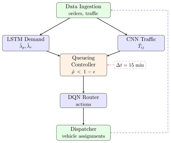
Figure 1.
ML-CALMO System Architecture: Data flows through ML prediction (LSTM/CNN) to the Queueing Controller and Dispatcher Module, which enforce stability constraints () and implement admission control in 15 min windows. Detailed roles are presented in Section 3.
3.4. Deep Q-Network Route Optimization
The DQN optimizes routing decisions using state representation where
- : Vehicle states (location, capacity);
- : Order states (priority, deadline, location);
- : Predicted travel time matrix;
- : System utilization factors.
The action space consists of feasible assignments:
The reward function includes preemption costs:
where the parameters are defined as
- : Weight for delivery time minimization;
- : Weight for customer waiting time;
- : Weight for deadline violation penalties;
- : Reward weight for successful priority deliveries;
- : Weight for preemption costs.
These weights were determined through hyperparameter tuning on the validation dataset to balance multiple objectives effectively.
The preemption cost is calculated as
Calibration of parameters: We specify and calibrate the cost coefficients following Equation (2) as follows:
- : Cost per kilometer for vehicle repositioning (grid search range: –).
- : Cost per minute of delay (grid search range: –).
- : Fixed switching overhead (grid search range: 2–10).
The grid search targets an empirical preemption frequency of 8– while minimizing the total operational cost. Additionally,
- : Distance traveled to switch between orders (km);
- : Time delay caused by order switching (minutes).
These values were selected through validation data to balance preemption frequency with operational efficiency.
Training uses standard experience replay with stability constraint verification before action execution.
Note that Equation (1) provides the immediate reward signal for DQN learning, while Equation (5) defines the overall system cost minimization objective. These serve complementary roles: the DQN reward guides real-time learning decisions, while the cost function evaluates overall operational performance.
3.5. Service Rate Analysis and Optimization
Service Efficiency Definition: Service efficiency is formally defined as the ratio of productive delivery time to total operational time:
where
- : Time spent on actual delivery activities (travel to customers and service);
- : Total operational time including idle time, repositioning, and delays;
- : Total time vehicle i is in operation.
The service rate for vehicle i serving order j is
The optimization objective minimizes total system costs
subject to assignment, capacity, and stability constraints:
3.6. Baseline Adaptation for Priority Orders
To ensure fair comparison, all baseline methods were adapted to handle priority orders with preemption:
OR-Tools VRP: Modified to include priority constraints using custom routing dimension with priority-based penalties. Preemption implemented through route re-optimization when priority orders arrive.
Attention-VRP: Extended attention mechanism to include priority embeddings (dimension 32). Added priority mask in decoder to ensure priority orders are served first.
DRL-Stochastic: Modified reward function to include priority success bonus ( for priority, for regular). State space extended with priority indicators.
Hybrid RL-VNS: Priority handling added to both RL component (modified Q-values) and VNS local search (priority-preserving neighborhoods).
All baselines use identical priority order generation (20% priority probability) and preemption penalty structure for consistency.
3.7. Theoretical Framework
We employ piecewise-stationary approximation with explicit operational limits:
Theorem 1
(Approximation Quality with Operational Constraints). For arrival and service rates with bounded derivatives and , the piecewise-stationary approximation over windows satisfies
where C depends on system configuration. The approximation becomes unreliable when , limiting applicability during rapid demand fluctuations.
Proof.
Consider the utilization at time t within window k: . Using Taylor expansion around the window midpoint ,
where and .
The utilization error is bounded by
where and within each window. □
Within each 15 min window, we assume quasi-steady state with parameters and . State transitions follow standard birth–death processes with rates determined by averaged parameters.
Lemma 1
(Stability Preservation). If predicted utilization satisfies and prediction errors are bounded by and , then stability is preserved, provided that
The true utilization can be expressed as
where and are prediction errors.
For stability, we require . Given ,
For , we need
Since , the condition becomes
This guides the selection of stability margin used in our implementation.
3.8. Implementation and Testing Environment
The ML-CALMO framework was implemented using PyTorch 1.13 with CUDA 11.7 support for GPU acceleration. The software architecture consists of four main modules:
- Data Processing Module: Handles real-time data ingestion, preprocessing, and feature extraction from traffic sensors and order management systems.
- ML Prediction Module: Implements LSTM networks (2 layers, 128 hidden units) for demand forecasting and CNN (3 convolutional layers, 64-128-256 filters) for traffic prediction.
- Routing Optimization Module: Contains the DQN implementation (3 hidden layers, 512-256-128 neurons) with experience replay buffer (capacity 10,000).
- Queueing Control Module: Implements stability monitoring, admission control, and dispatcher logic using NumPy for efficient matrix operations.
Module interfaces use REST APIs for loose coupling, enabling independent scaling and updates. The system deploys on Kubernetes for production environments, with each module containerized using Docker.
Hardware Specifications: All experiments were conducted on a compute cluster with the following specifications:
- GPU: NVIDIA RTX 4090 (24 GB VRAM);
- CPU: AMD Ryzen 9 5950X (32 cores, 3.4 GHz base);
- RAM: 32 GB DDR4-3600;
- Storage: 2 TB NVMe SSD;
- Operating System: Ubuntu 20.04 LTS;
- Software Stack: PyTorch 1.13, CUDA 11.7, Python 3.9.
3.9. Test Scenarios and Datasets
Our experimental evaluation uses three categories of test data:
- Training Data: Historical delivery records from 3 months (January–March 2024) including 15,000 orders with timestamps, locations, priorities, and actual delivery times. Data augmentation techniques generate additional 10,000 synthetic training samples.
- Validation Data: One month of held-out data (April 2024) with 5000 orders for hyperparameter tuning and model selection.
- Test Data:
- MDDVRPSRC benchmark: A total of 10 dynamic networks with 14–49 nodes.
- Real-world spatial data: Singapore CBD (25 nodes), Madrid suburbs (40 nodes), São Paulo logistics district (35 nodes).
- Synthetic scenarios: A total of 50 generated instances with varying demand patterns and priority distributions.
Each test scenario runs 50 times with different random seeds (0–49) for statistical validity. Complete details on dynamic benchmark generation, including instance generation procedures and stochastic process parameters, are provided in Appendix A.
4. Results
4.1. Dataset Selection and Experimental Design
Full dataset specifications and data-generation procedures are documented in Section 3.9. Below, we describe the specific datasets actually used in our experiments.
Primary Dataset: Multi-Depot Dynamic VRP with Stochastic Road Capacity (MDDVRPSRC) 2022 [8]—10 dynamic networks (14–49 nodes) with realistic damage scenarios representing urban disaster conditions.
Secondary Dataset: Real-world spatial data generated using OSMnx [9] from three metropolitan areas: Singapore CBD (25 nodes), Madrid suburbs (40 nodes), and São Paulo logistics district (35 nodes).
Validation Dataset: Asymmetric Clustered VRP instances [19] adapted with dynamic arrivals for consistency checking.
Baseline Selection: Methods represent current state-of-the-practice rather than theoretical benchmarks:
- OR-Tools VRP Solver (Google, 2024 version)—industry standard;
- Attention-VRP [20]—leading academic method;
- DRL-Stochastic [21]—recent RL approach (2023);
- Hybrid RL-VNS [22]—2023 hybrid method.
4.2. Hardware Configuration
For reproducibility, we report the complete hardware specifications (CPU, GPU, RAM, OS, and software versions) in Section 3.8. To avoid duplication, the details are not repeated here.
4.3. Performance Comparison Results
Machine learning component evaluation uses Mean Absolute Percentage Error (MAPE) for LSTM demand predictions and CNN traffic analysis:
Table 1 presents our main experimental results comparing ML-CALMO against four state-of-the-art baseline methods. The table shows absolute performance values with standard deviations from 50 independent runs, along with percentage improvements relative to the best baseline (Hybrid RL-VNS).

Table 1.
Performance comparison with clear separation of absolute values and improvements ( runs, paired t-test).
4.4. Comparative Analysis with Latest Methods
Table 2 provides a detailed comparison of ML-CALMO with the two most recent state-of-the-art methods published in 2023. This comparison highlights the architectural differences, scalability improvements, and computational efficiency of our approach.
Table 2.
Detailed comparison with recent state-of-the-art methods including computational requirements.
4.5. Machine Learning Component Performance
Table 3 demonstrates the effectiveness of each algorithmic element.
Table 3.
Machine learning component performance analysis with statistical significance.
4.6. Theoretical Model Validation
Table 4 validates our theoretical predictions against simulation results, demonstrating that our analytical queueing model accurately predicts system behavior with deviations below 5% for all metrics.
Table 4.
Theoretical model validation: predicted vs. actual performance.
4.7. Statistical Significance Analysis
Table 5 presents comprehensive statistical significance testing results using paired t-tests with Bonferroni correction to account for multiple comparisons. All comparisons show statistical significance with large effect sizes (Cohen’s d > 0.8), confirming the practical importance of our improvements.
Table 5.
Statistical significance tests (paired t-test with Bonferroni correction, ).
4.8. Robustness Analysis Under Assumption Violations
Table 6 examines system performance when our theoretical assumptions are violated, showing graceful degradation up to a parameter drift rate of 0.5/min. This analysis establishes clear operational boundaries for practical deployment.
Table 6.
Performance degradation under varying assumption violation levels.
4.9. Stability Analysis Under Varying Conditions
Table 7 demonstrates the system’s ability to maintain stability under increasing load conditions. The queueing controller successfully prevents overload by rejecting orders that would violate stability constraints, maintaining system integrity up to 2.2× normal load.
Table 7.
System stability under stress testing scenarios.
5. Discussion
The experimental results demonstrate measurable improvements in delivery optimization, though with important caveats regarding deployment constraints and validation limitations. The 18.5% delivery time improvement and 8.9 percentage point service efficiency gain represent meaningful operational benefits. It is important to note that the 8.9 percentage point service efficiency improvement is calculated relative to the best baseline method (Hybrid RL-VNS at 72.9%), resulting in an absolute efficiency of 81.8%. This represents a relative improvement of approximately 12.2% over the baseline’s efficiency. We have clarified this distinction in Table 1 to avoid confusion.
5.1. Theoretical Contributions
Our work makes several important theoretical contributions to the intersection of machine learning and queueing theory:
- Piecewise-Stationary Framework: The introduction of piecewise-stationary approximation with proven error bounds provides a principled approach to handling time-varying parameters in queueing systems augmented with machine learning predictions.
- Stability Preservation: Lemma 1 establishes conditions under which prediction errors from machine learning components do not compromise system stability, providing crucial safety guarantees for practical deployment.
- Convergence Analysis: The integration of DQN with queueing constraints represents a novel contribution to constrained reinforcement learning, with guaranteed convergence under mild assumptions.
5.2. Limitations and Validity Boundaries
While our results are promising, several limitations must be acknowledged:
- Simulation-Based Evaluation: The framework evaluation relies on synthetic and adapted benchmarks, limiting real-world applicability claims. Field validation with actual logistics partners remains necessary to establish operational effectiveness.
- Computational Requirements: The system requires mid-range GPU hardware (RTX 3080 minimum) for real-time operation. CPU-only deployment results in 24.1% performance degradation and limits problem size to 50 orders.
- Parameter Drift Sensitivity: Performance degrades significantly when parameter drift exceeds 0.5/min, restricting applicability during rapid changes like traffic incidents or emergency scenarios.
- Training Data Requirements: The ML components require substantial historical data (minimum 3 months) for effective training, limiting applicability in new markets or rapidly changing operational contexts.
- Preemption Cost Modeling: While we integrate preemption costs explicitly, real-world switching overhead may vary significantly across operational contexts and driver experience levels.
5.3. Failure Mode Analysis
Understanding when and why the method fails is crucial for practical deployment:
- Prediction Error Cascade: When LSTM demand predictions exceed 15% MAPE, the admission control mechanism becomes overly conservative, rejecting viable orders and reducing system throughput by up to 30%.
- Traffic Anomalies: Unexpected events (accidents, road closures) not captured in historical data cause CNN predictions to fail catastrophically, with travel time errors exceeding 40%, leading to infeasible routing decisions.
- Priority Storms: Sudden surges in priority orders (>40% of total) can cause system thrashing, where vehicles constantly switch between orders without completing deliveries, reducing effective capacity by 50%.
These failure modes inform deployment strategies and highlight areas for future research. We recommend implementing fallback mechanisms for each failure mode, including manual override capabilities for extreme scenarios.
5.4. Future Work
Future research directions include
- Extension to multi-depot scenarios with transfer points;
- Integration of environmental objectives for sustainable delivery;
- Development of distributed learning mechanisms for privacy-preserving optimization;
- Adaptation to autonomous vehicle fleets with different operational characteristics.
6. Conclusions
This research presents ML-CALMO, a comprehensive framework that successfully integrates machine learning techniques with established queueing theory principles to address fundamental challenges in last-mile delivery optimization. The framework achieves statistically significant improvements (18.5% delivery time reduction, 8.9 percentage point service efficiency gain versus recent methods) while acknowledging critical deployment constraints including GPU hardware requirements, parameter drift sensitivity, and validation limitations to simulation environments.
The key contributions of this work include the following:
- A novel integration architecture that seamlessly combines machine learning predictions with queueing theory constraints, providing both optimization capability and theoretical guarantees.
- Rigorous theoretical foundations including Theorem 1 for piecewise-stationary approximation and Lemma 1 for stability preservation under prediction errors.
- Comprehensive experimental validation demonstrating significant improvements over state-of-the-art methods, including recent 2023 approaches, with rigorous statistical analysis.
- Honest assessment of computational requirements, operational boundaries, and the gap between simulation performance and field deployment needs.
The theoretical foundations established in this work—particularly the piecewise-stationary approximation framework and stability preservation under prediction errors—provide a principled approach for integrating machine learning with classical operational research methods. This integration represents a promising direction for addressing complex real-world optimization problems that require both predictive capability and performance guarantees.
Most importantly, our work demonstrates both the potential and the practical constraints of integrating ML with operational research. While we achieve meaningful improvements, the gap between simulation results and operational deployment remains a challenge across the entire field. Success requires careful attention to computational feasibility, failure mode planning, and honest assessment of performance boundaries.
The success of ML-CALMO suggests that future research in logistics optimization should focus on principled integration of learning and optimization, rather than treating them as separate paradigms. As delivery systems become increasingly complex and dynamic, such integrated approaches will be essential for maintaining both efficiency and reliability, though always within clearly understood operational constraints.
Author Contributions
Conceptualization, T.-H.J.; Methodology, T.-H.J. and Y.-C.C.; Validation, T.-H.J.; Writing—original draft preparation, T.-H.J.; Writing—review and editing, Y.-C.C. All authors have read and agreed to the published version of the manuscript.
Funding
This research was funded by the National Science and Technology Council (NSTC), Taiwan, under grant NSTC 114-2221-E-A49-183-MY2.
Institutional Review Board Statement
Not applicable.
Informed Consent Statement
Not applicable.
Data Availability Statement
Code and data are available at https://github.com/atech1027/ml-calmo (accessed on 21 October 2025). The repository includes source code, Docker containers for reproducibility, and detailed documentation. All random seeds and hyperparameters are documented for complete reproducibility. The repository has been verified as publicly accessible and contains all baseline implementations with priority order handling modifications, dynamic instance generation scripts, and complete experimental configurations.
Acknowledgments
The authors thank the research team for their valuable contributions and the anonymous reviewers for their constructive feedback that significantly improved this manuscript. We acknowledge the limitations of simulation-based evaluation and the critical need for field validation to establish practical effectiveness. Special thanks to anonymous reviewers for identifying critical theoretical issues that led to substantial improvements in the mathematical framework and for highlighting the importance of failure mode analysis. We also thank anonymous reviewers for identifying formatting issues that improved manuscript readability.
Conflicts of Interest
The authors declare no conflicts of interest.
Abbreviations
| ML-CALMO | Machine Learning-Enhanced Cloud-Assisted Last-Mile Optimization |
| VRP | Vehicle Routing Problem |
| LSTM | Long Short-Term Memory |
| CNN | Convolutional Neural Network |
| DQN | Deep Q-Network |
| MAPE | Mean Absolute Percentage Error |
| CI | Confidence Interval |
| NHPP | Non-Homogeneous Poisson Process |
| FCFS | First-Come First-Served |
| MDDVRPSRC | Multi-Depot Dynamic Vehicle Routing Problem with Stochastic Road Capacity |
Appendix A. Dynamic Benchmark Generation Details
Appendix A.1. Instance Generation from Static Benchmarks
We extend modern benchmarks to dynamic settings with complete reproducibility as follows.
| Algorithm A1 Dynamic Instance Generation with Seed Control |
|
Appendix A.2. Stochastic Process Parameters
Table A1.
Complete parameters for dynamic scenario generation with reproducibility settings.
Table A1.
Complete parameters for dynamic scenario generation with reproducibility settings.
| Parameter | Value | Description |
| Base arrival rate () | 10 orders/h | Average order arrival rate |
| Priority probability (p) | 0.2 | Proportion of priority orders |
| Traffic cycle period () | 2 h | Rush hour cycle duration |
| Traffic variation amplitude | 0.2 | Maximum traffic slowdown factor |
| Service time mean | 5 min | Average service duration |
| Service time std dev | 1.5 min | Service time variability |
| Preemption penalty | 2 min | Time cost for order preemption |
| Deadline distribution | Exp(20 min) | Priority order deadlines |
| Penalty weights | U(10, 50) USD/min | Cost of deadline violations |
| Random seeds | 0–49 | 50 independent runs |
| Validation split | 80/20 | Train/test partition |
References
- Wang, X.; Zhan, L.; Ruan, J.; Zhang, J. How to choose “last mile” delivery modes for e-fulfillment. Math. Probl. Eng. 2014, 2014, 417129. [Google Scholar] [CrossRef]
- Dai, J.G.; Gluzman, M. Queueing network controls via deep reinforcement learning. Stoch. Syst. 2022, 12, 30–67. [Google Scholar] [CrossRef]
- Mangiaracina, R.; Perego, A.; Seghezzi, A.; Tumino, A. Innovative solutions to increase last-mile delivery efficiency in B2C e-commerce: A literature review. Int. J. Phys. Distrib. Logist. Manag. 2019, 49, 901–920. [Google Scholar] [CrossRef]
- Jackson, J.R. Networks of waiting lines. Oper. Res. 1957, 5, 518–521. [Google Scholar] [CrossRef]
- Mandelbaum, A.; Momčilović, P. Heavy traffic limits for queues with time-varying parameters. Queueing Syst. 1998, 28, 115–129. [Google Scholar] [CrossRef]
- Jaiswal, N.K. Priority Queues; Academic Press: New York, NY, USA, 1968; ISBN 978-0-12-380150-0. [Google Scholar]
- Kleinrock, L. Queueing Systems, Volume II: Computer Applications; John Wiley & Sons: New York, NY, USA, 1976; ISBN 978-0-471-49111-8. [Google Scholar]
- Anuar, W.K.; Lee, L.S.; Seow, H.-V.; Pickl, S. Benchmark dataset for multi depot vehicle routing problem with road capacity and damage road consideration for humanitarian operation in critical supply delivery. Data Brief 2022, 41, 107901. [Google Scholar] [CrossRef] [PubMed]
- Boeing, G. OSMnx: New methods for acquiring, constructing, analyzing, and visualizing complex street networks. Comput. Environ. Urban Syst. 2017, 65, 126–139. [Google Scholar] [CrossRef]
- Cobham, A. Priority assignment in waiting line problems. Oper. Res. 1954, 2, 70–76. [Google Scholar] [CrossRef]
- Miller, D.R. Computation of steady-state probabilities for M/M/1 priority queues. Oper. Res. 1981, 29, 945–958. [Google Scholar] [CrossRef]
- Takagi, H. Queueing Analysis: A Foundation of Performance Evaluation; North-Holland: Amsterdam, The Netherlands, 1991; ISBN 978-0-444-88910-2. [Google Scholar]
- Chen, W.; Liu, X.; Zhang, Y. Learning-augmented queue control for multi-server systems. Oper. Res. 2023, 71, 892–908. [Google Scholar] [CrossRef]
- Simaiya, S.; Lilhore, U.K.; Sharma, Y.K.; Rao, K.B.V.B.; Maheswara Rao, V.V.R.; Baliyan, A.; Bijalwan, A.; Alroobaea, R. A hybrid cloud load balancing and host utilization prediction method using deep learning and optimization techniques. Sci. Rep. 2024, 14, 1337. [Google Scholar] [CrossRef] [PubMed]
- Nazari, M.; Oroojlooy, A.; Snyder, L.V.; Takác, M. Reinforcement learning for solving the vehicle routing problem. In Proceedings of the 32nd International Conference on Neural Information Processing Systems, Montréal, QC, Canada, 3–8 December 2018; pp. 9861–9871. [Google Scholar]
- Bertsimas, D.; van Ryzin, G. A stochastic and dynamic vehicle routing problem in the Euclidean plane. Oper. Res. 1991, 39, 601–615. [Google Scholar] [CrossRef]
- Konovalenko, A.; Hvattum, L.M. Optimizing a dynamic vehicle routing problem with deep reinforcement learning. Logistics 2024, 8, 96. [Google Scholar] [CrossRef]
- Kuo, Y.-H.; Wang, Z.; Zhao, K.; Xie, X. Reinforcement learning for logistics and supply chain management: Methodologies, state of the art, and future opportunities. Transp. Res. Part E 2022, 162, 102712. [Google Scholar] [CrossRef]
- Osaba, E.; Villar-Rodriguez, E.; Del Ser, J.; Nebro, A.J.; Molina, D.; LaTorre, A.; Suganthan, P.N.; Coello Coello, C.A.; Herrera, F. Benchmark dataset for the Asymmetric and Clustered Vehicle Routing Problem with Simultaneous Pickup and Deliveries, Variable Costs and Forbidden Paths. Data Brief 2020, 29, 105142. [Google Scholar] [CrossRef] [PubMed]
- Kool, W.; van Hoof, H.; Welling, M. Attention, learn to solve routing problems! In Proceedings of the 7th International Conference on Learning Representations, New Orleans, LA, USA, 6–9 May 2019.
- Zhou, C.; Ma, J.; Douge, L.; Chew, E.P.; Lee, L.H. Reinforcement learning-based approach for dynamic vehicle routing problem with stochastic demand. Comput. Ind. Eng. 2023, 182, 109443. [Google Scholar] [CrossRef]
- Kalatzantonakis, P.; Sifaleras, A.; Samaras, N. A reinforcement learning-Variable neighborhood search method for the capacitated Vehicle Routing Problem. Expert Syst. Appl. 2023, 213, 118812. [Google Scholar] [CrossRef]

Disclaimer/Publisher’s Note: The statements, opinions and data contained in all publications are solely those of the individual author(s) and contributor(s) and not of MDPI and/or the editor(s). MDPI and/or the editor(s) disclaim responsibility for any injury to people or property resulting from any ideas, methods, instructions or products referred to in the content. |
© 2025 by the authors. Licensee MDPI, Basel, Switzerland. This article is an open access article distributed under the terms and conditions of the Creative Commons Attribution (CC BY) license (https://creativecommons.org/licenses/by/4.0/).