Article

A Comparative Analysis of Preprocessing Filters for Deep Learning-Based Equipment Power Efficiency Classification and Prediction Models

1
Department of Biomedical Engineering, Ulsan National Institute of Science and Technology, Ulsan 44919, Republic of Korea
2
SCT Co., Ltd., Busan 48059, Republic of Korea
3
Department of Mathematics and Statistics, Old Dominion University, Norfolk, VA 23529, USA
4
Department of Management Information Systems, Dong-A University, Busan 49236, Republic of Korea
*
Author to whom correspondence should be addressed.
These authors contributed equally to this work.
Appl. Sci. 2025, 15(20), 11277; https://doi.org/10.3390/app152011277
Submission received: 11 September 2025 / Revised: 16 October 2025 / Accepted: 20 October 2025 / Published: 21 October 2025

Abstract

The quality of input data is critical to the performance of time-series classification models, particularly in the domain for industrial sensor data where noise and anomalies are frequent. This study investigates how various filtering-based preprocessing techniques impact the accuracy and robustness of a Transformer model that predicts power efficiency states (Normal, Caution, Warning) from minute-level IIoT sensor data. We evaluated five techniques: a baseline, Simple Moving Average, Median filter, Hampel filter, and Kalman filter. For each technique, we conducted systematic experiments across time windows (360 and 720 min) that reflect real-world industrial inspection cycles, along with five prediction offsets (up to 2880 min). To ensure statistical robustness, we repeated each experiment 20 times with different random seeds. The results show that the Simple Moving Average filter, combined with a 360 min window and a short-term prediction offset, yielded the best overall performance and stability. While other techniques such as the Kalman and Median filters showed situational strengths, methods focused on outlier removal, like the Hampel filter, adversely affected performance. This study provides empirical evidence that a simple and efficient filtering strategy such as Simple Moving Average, can significantly and reliably enhance model performance for power efficiency prediction tasks.

1. Introduction

The proliferation of Internet of Things (IoT) devices in real-time sensor data acquisition environments has highlighted the critical importance of power efficiency management [1]. Many companies are collecting and leveraging vast amounts of time-series data to reduce operational costs and enhance system reliability through predictive maintenance [2]. At the core of this data-driven approach are AI-based time-series classification models, which analyze raw sensor data to support proactive decision-making [3]. In particular, recently proposed deep learning-based time-series analysis models have received significant attention from both academia and industry for their ability to effectively capture long-term temporal dependencies within data [4,5].
However, most existing academic research tends to assume ideal data conditions, often focusing on model architecture improvements using clean, small-scale, and impractical public datasets [6]. In practice, sensor data from industrial settings are susceptible to various imperfections, including high-frequency noise, outliers, and signal loss, which arise from interference, malfunctions, and environmental factors. Cleaning this noisy data is a fundamental and necessary step for accurate analysis [7]. Without proper cleaning, even the most advanced models are likely to produce a high number of false positives and unreliable results [7]. This reality creates an inherent limitation where the performance of any predictive model is ultimately capped by the quality of its input data [6,8]. Consequently, even sophisticated deep learning models with numerous parameters are prone to learning spurious patterns or exhibiting degraded predictive performance when applied directly to raw, noisy data.
In response to the inherent limitations of this ‘model-centric’ paradigm, this study proposes a fundamental shift in focus. This study directly challenges the prevailing research trend of pursuing ever-increasing model complexity and argues that a ‘data-centric’ approach, which prioritizes the quality of input data, offers a more robust and practical solution. Specifically, it hypothesizes that even a state-of-the-art model is ineffective when faced with noisy data, and that applying computationally efficient and interpretable traditional filtering techniques is a more impactful strategy for improving both model performance and stability. To empirically validate this hypothesis, this study systematically evaluates the impact of various filtering techniques on two representative deep learning models with contrasting architectural philosophies: the complex, attention-based Transformer and the simple yet powerful linear-based R-Linear. This comparison is designed to highlight the critical trade-off between state-of-the-art architectures and lightweight, industry-friendly alternatives. Both models are tested using real-world industrial power efficiency data. The key contributions of this study are as follows:
  • Challenging Model-Centrism: Through extensive experiments on a real-world industrial power-efficiency dataset, the study empirically demonstrates that a data-centric preprocessing approach yields more significant and robust performance gains than relying on model complexity, validated across diverse architectures like the Transformer and R-Linear.
  • The Surprising Effectiveness of Simplicity: Grounded in our empirical analysis, the study reveals the counter-intuitive result that the Simple Moving Average (SMA)—a traditional and efficient filter—consistently outperforms more complex filtering techniques on real-world industrial data.
  • A Practical Framework for Preprocessing: Based on the comprehensive results of our scenario-based experiments, the study provides an empirically validated framework that offers actionable guidelines for practitioners to select optimal filtering strategies by analyzing the trade-offs between performance, stability, and window sizes.
This paper is organized as follows. Section 2 reviews prior literature related to power efficiency diagnostics. Section 3 describes the dataset and the research methodology utilized in this study. Section 4 presents the experimental results for each scenario, and Section 5 and Section 6 provide discussion and conclusion, respectively.

2. Related Works

2.1. Data-Driven Approaches for Industrial Predictive Maintenance

In modern manufacturing, data-driven predictive maintenance has become a critical strategy for enhancing system reliability and operational efficiency. A prime example of this paradigm can be found in the complex task of estimating a battery’s State of Health (SOH), which is crucial for the safety of many Industrial Internet of Things (IIoT) systems [9,10]. SOH is a quantitative indicator that reflects the extent to which a battery’s performance has degraded compared to its original state [11]. It is not a parameter that can be directly measured by sensors; rather, it must be inferred and estimated from observable operational data such as voltage, current, and temperature [12]. Traditional SOH estimation research relied on physics-based approaches, such as the Equivalent Circuit Model (ECM), which attempted to mathematically model the internal electrochemical processes of a battery. However, battery degradation exhibits highly complex and non-linear characteristics influenced by various factors such as aging, charge–discharge patterns, and temperature. Consequently, physics-based models have clear limitations in accurately capturing these multi-dimensional dynamics [13].
These limitations have driven a paradigm shift toward data-driven methodologies for SOH estimation. This approach seeks to overcome the shortcomings of traditional methods by using deep learning architectures—such as CNNs, LSTMs, and transformers—to directly learn complex non-linear relationships from operational data such as voltage, current, and temperature [14]. A key advantage is the ability to model degradation behavior without requiring an explicit and complete understanding of the underlying electrochemical physics [15]. This flexibility enables high accuracy and adaptability, often leading to performance that surpasses traditional models, particularly when large datasets are available [16]. However, the performance of these deep learning models is highly dependent on the quality of the input data. Sensor data collected from real-world industrial settings inevitably contains noise and outliers, which can severely impact a model’s accuracy and stability [8]. The challenges observed in SOH estimation, particularly the critical dependency on high-quality input data, are not unique to this domain. Indeed, they represent pervasive issues across a wide range of industrial predictive maintenance tasks, including monitoring the energy efficiency of automated manufacturing processes and diagnosing performance degradation in heavy industrial machinery.

2.2. Deep Learning Models for Industrial Time-Series Analysis

The development of deep learning-based models for industrial time-series analysis is a field of active research. Early studies primarily adopted Recurrent Neural Network (RNN) architectures such as LSTM and GRU to effectively learn the temporal dependencies in battery cycle data [17,18]. However, these models, due to their sequential processing nature, have limitations in terms of difficulty with parallelization and degraded learning efficiency as the input time series becomes longer [19].
Subsequently, transformer-based models attracted significant attention for their ability to effectively process long-range dependencies in parallel through the attention mechanism [20]. Related research has explored various architectural innovations beyond the standard Transformer encoder [21]. For instance, hybrid models such as the CNN-Transformer, which captures both local features and global context simultaneously, and the LSTM-Transformer have been proposed [22,23]. Concurrently, several modifications to the conventional transformer architecture have been attempted the iTransformer, for example, was designed with a variable-centric attention structure to handle irregularly sampled raw data [24]. More recently, foundation models such as DiffBatt have also been introduced, which are pre-trained on diverse battery datasets and then fine-tuned for specific tasks [25].
However, a recent line of research has begun to question whether this trend toward ever-increasing model complexity is always necessary. In contrast, several studies have formed a new research stream by demonstrating that surprisingly simple, linear-based models can achieve competitive performance on various time-series tasks. The pioneering N-Linear and D-Linear models led this trend by proposing approaches to handle distribution shifts and separately model trend and seasonality through normalization and time-series decomposition techniques, respectively [26]. Inheriting this philosophy, the R-Linear model—despite its extremely simple structure consisting only of a single linear layer and normalization—has established itself as a powerful baseline that performs comparably or better than complex models [27]. This emerging trend, represented by models such as N-Linear, D-Linear, and R-Linear, suggests a renewed focus on fundamental model properties over sheer architectural complexity.
This architecture-centric research trend reveals a significant research gap. While there is an active debate surrounding complex Transformer-based and simple linear-based models, research on pre-processing—which fundamentally affects the performance of both—is lacking. For instance, there has been little experimental analysis on how traditional techniques for noise suppression, such as the Simple Moving Average (SMA) or Median filters, impact the performance and stability of these deep learning models in real-world industrial data environments [28,29]. To fill this gap, this study conducts a data-centric empirical analysis that focuses on the impact of input data quality rather than the complexity of the model architecture.

2.3. Filtering Methodologies for Time-Series Preprocessing

Filtering is a key signal processing technique used to mitigate inherent noise and anomalies in time-series data before model training. The choice of a filter imparts a specific inductive bias to the model. Therefore, it is crucial to select a methodology that aligns with the statistical characteristics of the data being analyzed. Since the industrial time-series data in this study contains both random noise and transient outliers from various variables, we compare and analyze the following diverse filtering methodologies. To establish a baseline for comparison, we also evaluated the model on the original, unprocessed data.

2.3.1. SMA

SMA is a linear filter that calculates the arithmetic mean of consecutive data points within a sliding window of a specified size [28]. The SMA value at a specific time point t is calculated as shown in Equation (1),
S M A t = 1 N i = t N + 1 t x i
Here, x i ’s represents the observed value of the time-series data, and N denotes the window size for the moving average calculation. This produces the simple moving average value at time t based on the sum of the past N data points. The primary advantages of SMA are its implementation simplicity and computational efficiency. However, it is sensitive to outliers, which can distort the average because it assigns equal weight to all data points within the window. As a result, in segments where the signal changes abruptly, it may fail to adequately reflect the characteristics of the original data [30].

2.3.2. Median Filter

The Median Filter is a non-linear technique that replaces each data point with the median of its neighboring values within a sliding window [29]. The formula for applying the Median Filter is as follows in Equation (2),
y t = M e d i a n ( x t k ,   , x t , , x t + k )
Here, y t represents the final filtered output value at a specific time t . It is determined by identifying and using the median value from the set of original data points within the sliding window centered at time t . Its primary strength is the robustness to impulse noise and outliers [31]. It also excels at preserving sharp edges and step functions in the signal, which are critical features in battery charge cycles.

2.3.3. Hampel Filter

The Hampel filter is a decision-based filter designed for outlier detection and replacement [32]. This filter identifies a data point as an outlier if it deviates from the median of its window by more than a threshold defined by the Median Absolute Deviation (MAD) [33]. The outlier is then replaced with the median value of the window. The Hampel filter is defined in Equation (3),
y t = m t ,   i f x t m t > γ M A D t x t , o t h e r w i s e
Here, y t is the raw data value at time t , and m t is the median of the central window. M A D t represents the Median Absolute Deviation of the central window, and points are considered outliers based on a threshold value γ . Because it uses robust statistical estimation, the Hampel filter is an effective technique for removing outliers without significantly distorting non-outlier data points [32].

2.3.4. Kalman Filter

Unlike simple filters that rely on statistical summaries of past data, the Kalman filter is a powerful recursive algorithm that estimates the dynamic state of a system [34]. It operates by constantly repeating two steps: ‘predict’ and ‘update’. First, it predicts the current state based on the system’s previous state. Then, it uses the actual measurement from the sensor to correct errors in the prediction, thereby updating to the most likely optimal state. The Kalman filter is defined in Equation (4),
x ^ t = x ^ t + K t z t x ^ t
Here, x ^ t is the posteriori state estimate at the current time t , and x ^ t is the a priori estimate predicted by the model based on the previous state. z t represents the actual measurement observed at time t . The key component, K t , is the Kalman Gain, which is an optimal weight calculated by considering the uncertainty of the prediction and the uncertainty of the measurement. Through this intelligent fusion of prediction and measurement, the Kalman filter can effectively remove noise in real-time, making it particularly useful for processing dynamic and non-stationary industrial data.

3. Experiments

3.1. Dataset

This study is based on a minute-level multivariate time-series dataset from the power systems of real-world industrial machine tools (HYUNDAI&KIA Machine, Goryeong, Republic of Korea). The dataset, to our knowledge, has not been previously reported in academic literature. The data was collected from 00:00 on 16 September 2020, to 23:59 on 22 October 2020. The dataset comprises 37 columns, including the collection timestamp, and contains various electrical signals and operational parameters such as power factor, active power, reactive power, current, and voltage. The dataset includes both normal and abnormal system states, which are classified based on the average power factor, as illustrated in Figure 1. The dataset and source code used in this study are available via the Data Availability Statement at the end of this paper.
The data used in this study is divided into three classes. The distribution of the data across these classes is shown in Table 1 below.
  • Normal: This class represents states where the system is operating within optimal efficiency parameters, indicated by an average power factor of 80% or higher.
  • Caution: This class indicates minor but significant deviations from optimal efficiency, suggesting that future maintenance may be required. This corresponds to an average power factor between 60% and 80%.
  • Warning: This class signifies a state of severe inefficiency that requires immediate attention, defined by an average power factor below 60%.

3.2. Pre-Processing Pipeline and Model Architecture

The experiments in this study are based on a systematic data processing pipeline. First, datasets are prepared, including the original raw version and versions processed by the various pre-processing filters. From each of these datasets, a sliding window technique is applied to generate input samples (X), which represent historical time series, and corresponding labels (y), which represent the power efficiency state at a future time point. This generated data is then used to train and evaluate two contrasting model architectures.
To comprehensively evaluate the impact of pre-processing, this study employs two models with contrasting philosophies. The primary model is a transformer, consisting of a single encoder block featuring a multi-head self-attention mechanism and a feed-forward network. Residual connections and layer normalization are applied to each sub-layer, and the encoder’s output is passed to a final classification head. As a counterpoint, an R-Linear model is used, which consists of a single fully connected linear layer that directly maps the flattened input from the time window to the final output.
The experimental scenarios were designed to simulate various industrial operational conditions and to comprehensively evaluate the performance and robustness of each pre-processing technique. The scenarios are constructed by combining two key parameters: the time window, which is the period of historical data the model references, and the prediction offset, which is the point in the future to be predicted.
The time window determines the amount of historical information the model learns from. This study establishes two scenarios reflecting actual industrial work cycles. The 360 min (6 h) window is intended to capture the dynamic state changes and operational patterns of equipment that occur within a typical half-day work shift. The 720 min (12 h) window is designed to allow the model to learn longer-term patterns that may span across shifts or relate to daily load variations. Longer windows were excluded from the scope of this study due to the practical constraint of significantly increased computational cost and memory requirements.
The prediction offset is directly linked to the practical application purpose of the predictive model. In this study, multiple offsets were set to simulate various decision-making horizons, from short-term anomaly detection to long-term maintenance planning. The 60 min (1 h), 360 min (6 h), and 720 min (12 h) offsets reflect ‘tactical planning’ to prepare for immediate actions by predicting the equipment’s state for the next work shift. In contrast, the 1440 min (24 h) and 2880 min (48 h) offsets represent ‘strategic maintenance’ scenarios that require advance planning, such as ordering spare parts or deploying personnel.
Through these systematically designed scenarios, we aim to comprehensively analyze how each pre-processing technique’s performance varies under different temporal contexts and prediction goals, thereby verifying its practical effectiveness.

3.3. Experimental Setup

All experiments were implemented in Python (v3.9.12), and the deep learning models were built using the PyTorch (v2.1.0) framework. Data manipulation and numerical operations were primarily handled by Pandas (v2.2.3) and NumPy (v1.24.4).
The filtering methods were implemented using established scientific libraries. The Simple Moving Average (SMA) was calculated using the rolling method in Pandas. The Median filter was applied using functions from the SciPy (v1.13.1) library. The Hampel filter was implemented using the Median Absolute Deviation (MAD) from the Statsmodels (v0.14.4) library, and the Kalman filter was implemented using the KalmanFilter class from the PyKalman (v0.10.2) library.
All experiments were conducted on a workstation running Windows 11 Pro, equipped with an Intel Core i9-10980XE CPU (Intel, Santa Clara, CA, USA), 128 GB of RAM, and an NVIDIA RTX 3090 GPU with 24 GB of VRAM (NVIDIA, Santa Clara, CA, USA). To ensure reproducibility, the source code is publicly available, as noted in the Data Availability Statement.

3.4. Evaluation

The entire dataset is split into a training set (80%) and a testing set (20%). Furthermore, to account for the inherent stochasticity of deep learning model training (e.g., weight initialization, data batching), and ensure the reliability of our results, we repeated each unique experimental configuration (a combination of a filter, time window, and offset) 20 times. Each repetition used a different random seed to ensure robust results. The model was trained for 100 epochs using the Adam optimizer with a batch size of 1024.
The classifier’s performance under each condition is evaluated using the following metrics. Through an analysis of the mean and standard deviation over the 20 runs, we empirically evaluate the average performance and stability. Additionally, the model’s training time is also recorded to compare computational efficiency.
  • A c c u r a c y : Measures the overall proportion of correctly classified instances across all three classes, as defined in Equation (5),
a c c u r a c y = N u m b e r   o f   c o r r e c t   p r e d i c t i o n s T o t a l   n u m b e r   o f   p r e d i c t i o n s
  • F 1   S c o r e : A key metric for imbalanced datasets, the F 1   S c o r e is the harmonic mean of P r e c i s i o n and R e c a l l . P r e c i s i o n measures the proportion of positive identifications that were actually correct, while R e c a l l measures the proportion of actual positives that were correctly identified. The F 1   S c o r e is then calculated with Equation (6). For this multi-class problem, the macro-averaged F 1   S c o r e is used.
    P r e c i s i o n = T P T P + F P R e c a l l = T P T P + F N F 1   S c o r e = 2 × P r e c i s o n × R e c a l l P r e c i s o n + R e c a l l
    where T P , F P , and F N represent True Positives, False Positives, and False Negatives, respectively.
  • Training Time: Measures the average training time for each iteration of the experiment.

4. Results

4.1. Experimental Results by Window Size

This section systematically analyzes the experimental results conducted under various scenarios. First, we compare the impact of input data length, i.e., the window size, on the model’s predictive performance to identify the optimal combination of scenarios for each preprocessing technique. Furthermore, by analyzing not only the mean performance but also the standard deviation from repeated experiments, we evaluate the stability and reliability of each model to assess its applicability in real-world industrial environments.

4.1.1. Results Based on a 360 min Window

The experimental results for the 360 min input window using the Transformer model are presented in Table 2. This table details both the mean performance and the standard deviation for each metric, enabling an in-depth analysis of each preprocessing technique’s characteristics, particularly its stability. The key findings are as follows:
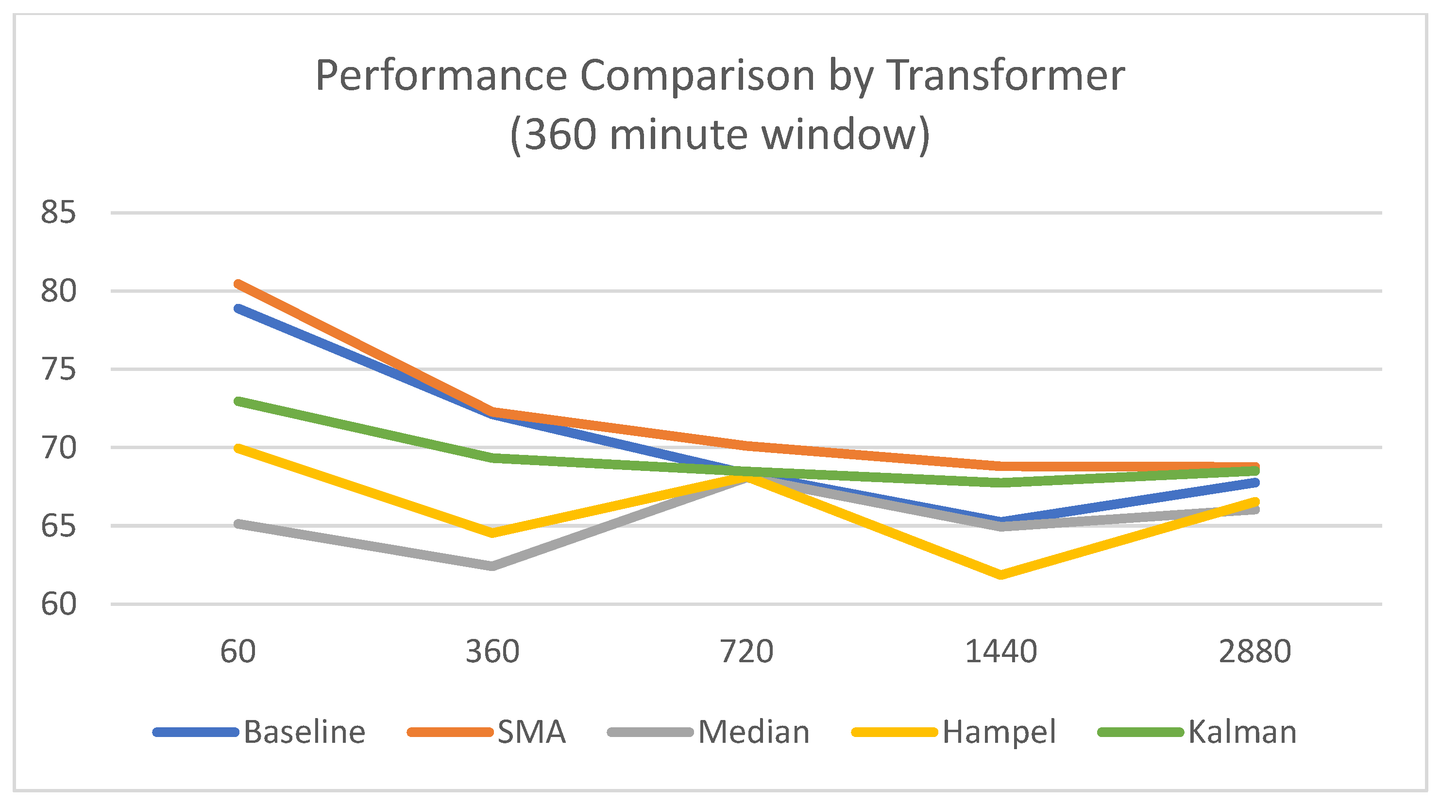
  • The Simple Moving Average (SMA) filter achieved the highest mean accuracy of 80.45% and the lowest standard deviation of 1.94%, establishing it as the most effective and reliable preprocessing technique for short-term predictions.
  • In contrast, other filters demonstrated clear limitations, particularly in terms of stability. The Median filter was highly unstable with an extreme accuracy standard deviation of 11.60%, and the Kalman filter also showed high instability in short-term predictions with a standard deviation of 10.62%.
  • A consistent trend emerged across most techniques where mean performance gradually decreased as the prediction offset became longer, highlighting the increased difficulty of long-term forecasting.
The baseline model (without preprocessing) recorded a respectable mean accuracy of 78.88% (Std. 4.26%) at the 60 min offset. However, the best overall results were observed with the SMA filter. It achieved the highest accuracy of 80.45% at the 60 min offset, coupled with the lowest standard deviation of 1.94%. This demonstrates that for short-term predictions, SMA is the most effective and reliable preprocessing technique tested.
In contrast, other filters exhibited clear limitations. The Median filter, for instance, was highly unstable, showing an extreme accuracy standard deviation of 11.60% at the 60 min offset. This suggests that the filter may excessively remove signals essential for learning, depending on the data batch or initial weights. The Hampel filter showed similarly high instability and lower overall performance. The Kalman filter presented a unique profile; while it was also highly unstable for short-term predictions (Std. 10.62%), its stability significantly improved at longer horizons, achieving a low standard deviation of 2.24% at the 2880 min offset. This implies that its model-based approach, while volatile in the short term, offers more consistent predictions for long-term forecasting.
Figure 2 illustrates the performance comparison of each pre-processing technique according to changes in the prediction offset, using a 360 min input window. As is clearly visible from the graph, the SMA filter, represented by the orange line, consistently maintained superior performance over the baseline and other filters across nearly all prediction intervals. It particularly demonstrated its effectiveness by achieving peak performance at the shortest-term prediction, the 60 min offset.
Additionally, a significant trend observed in the graph is that the accuracy of most techniques gradually decreases as the prediction offset lengthens. The fact that all techniques, including SMA, perform worse when predicting 2880 min ahead than 60 min ahead highlights the inherent challenge of time-series forecasting, where uncertainty increases with temporal distance to the target.
Table 3 shows the experimental results for the R-Linear model using a 360 min window. An analysis of these results reveals several key characteristics in comparison to the Transformer model:
  • The R-Linear model showed an overall decrease in performance compared to the Transformer model. Its peak accuracy was 75.15% with the Median filter, which was significantly lower than the Transformer’s peak of 80.45%.
  • Due to its simpler linear architecture, the R-Linear model was less sensitive to the different preprocessing techniques, resulting in smaller performance variations among them.
  • Despite lower sensitivity, data preprocessing still provided meaningful performance improvements. The Median filter was effective for short-term predictions, while the SMA technique showed improved accuracy for long-term predictions.
The most prominent feature compared to the Transformer model is the overall decrease in performance. While the R-Linear model’s accuracy peaked at 75.15% when using the Median filter, the Transformer model achieved a significantly higher peak accuracy of 80.45% when paired with its optimal pre-processing method, the SMA filter. This is also true for other preprocessing techniques.
Another notable characteristic is the significantly smaller performance variation among the different pre-processing techniques. This is analyzed to be due to the inherent nature of the R-Linear as a simple linear model; it is less sensitive to the subtle differences in data patterns created by various pre-processing methods.
Crucially, data pre-processing still provided meaningful performance improvements. For instance, the Median filter outperformed the Baseline in short-term prediction, and the SMA technique showed improved accuracy in long-term predictions (e.g., 1 day and 2 days ahead). This confirms the universal benefit of applying a data-centric pre-processing approach.
Figure 3 shows the performance of the R-Linear model with a 360 min input window across different prediction offsets. For 60 min offset predictions, the Median and Kalman filters provided a clear performance advantage over other techniques. In contrast, from the 1440 min offset onwards, the SMA-based preprocessing technique demonstrates superior performance. This indicates that the optimal filter for the R-Linear model is dependent on the prediction horizon.

4.1.2. Results Based on a 720 min Window

The experimental results for the extended 720 min input window, presented in Table 4, reveal a significant overall degradation in both predictive performance and model stability. The analysis of this inefficient input scenario highlights the following key points:
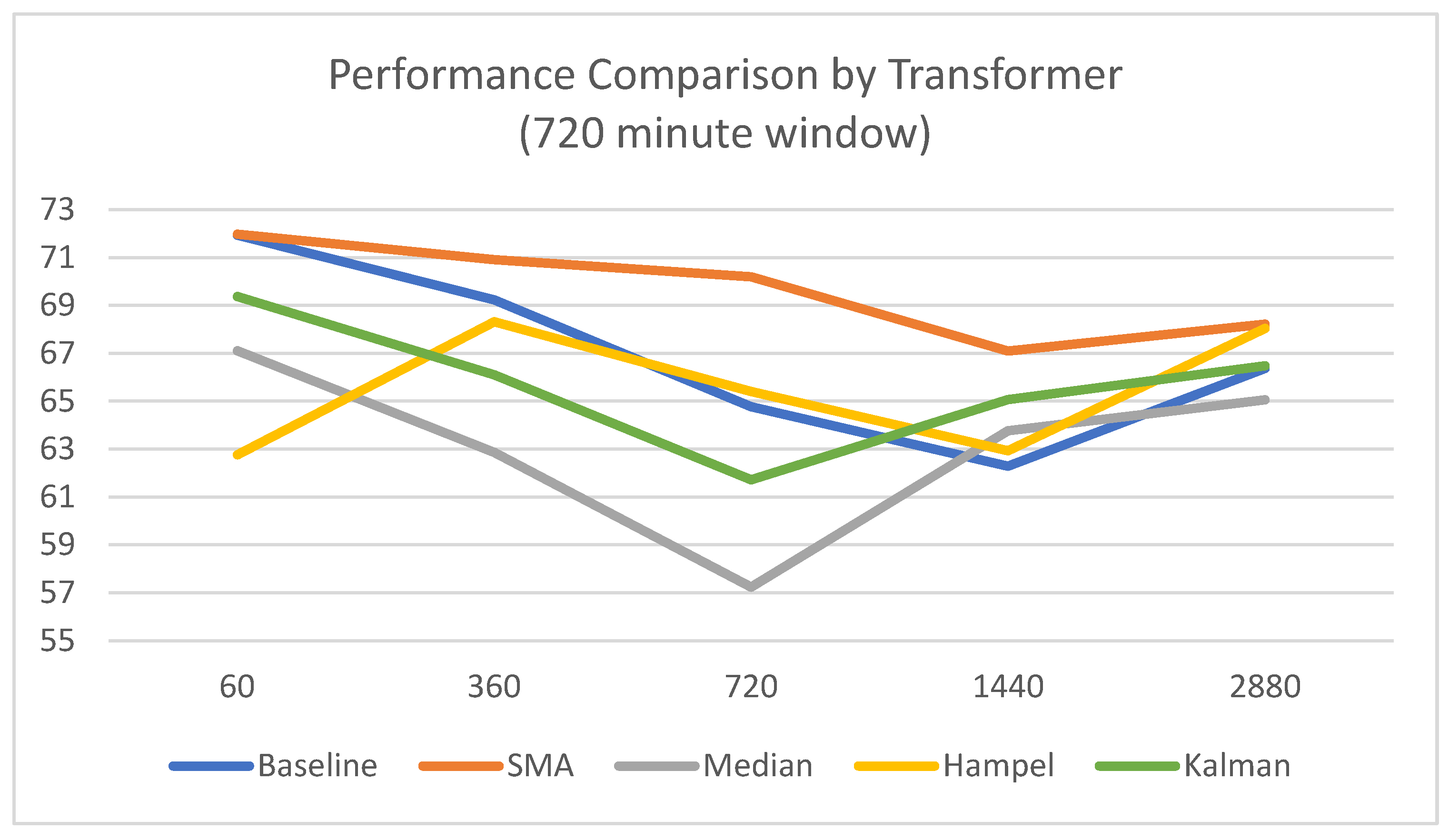
  • The longer window degraded performance, with the baseline model’s peak accuracy dropping to 71.94% and its stability decreasing significantly with a standard deviation as high as 12.03%. This supports the hypothesis that excessively long windows can introduce performance-hindering noise.
  • The SMA filter achieved the highest mean accuracy (71.98%) but exhibited significant instability in short-term predictions, with a high standard deviation of 13.73%.
  • Other preprocessing methods, including Median, Hampel, and Kalman, failed to surpass the baseline in terms of mean accuracy and consistently showed elevated standard deviations, confirming they were ineffective in this scenario.
The experimental results for the extended 720 min input window, presented in Table 4, clearly show a significant overall degradation in both predictive performance and model stability when compared to the 360 min window scenario. The peak accuracy of the baseline model dropped to 71.94%, and it exhibited considerable instability, particularly in mid-term predictions, with the accuracy standard deviation reaching as high as 12.03 at the 720 offset. This result strongly supports the hypothesis that an excessively long input window, rather than improving performance, introduces noise and irrelevant historical data that complicates the learning process, ultimately degrading both the model’s accuracy and stability.
Under these inefficient input conditions, the effectiveness of each pre-processing technique also varied. Even the SMA filter, previously optimal, exhibited inconsistent performance. Although it achieved a mean accuracy of 71.98%, comparable to the baseline, it became highly unstable in short-term predictions, with its standard deviation reaching 13.73%. In contrast, the other pre-processing methods, including Median, Hampel, and Kalman, not only failed to surpass the baseline in terms of mean accuracy but also consistently showed elevated standard deviations, confirming they were both ineffective and unreliable in this scenario.
Nevertheless, the SMA filter reaffirmed its status as the most stable alternative by consistently exhibiting performance comparable to or slightly better than the baseline, even in this scenario. This result strongly supports the hypothesis that when the input data length becomes excessively long, it may contain irrelevant noise or less pertinent information, thereby hindering the model’s learning process.
Figure 4 illustrates the experimental results when the input data length was extended to 720 min. The primary observation is the overall decline in predictive performance compared to the 360 min window scenario. The peak performance of the baseline model only reached approximately 72%, a significant decrease from the 360 min window scenario. This suggests that an excessively long input window introduces irrelevant historical information that acts as noise, hindering the model’s ability to learn meaningful patterns.
Furthermore, this approach was computationally inefficient. As the input length doubled, the average training time also nearly doubled, making it an impractical choice. Therefore, when considering both predictive accuracy and computational cost, the 720 min window was determined to be an ineffective scenario for this task.
Table 5 shows the results of applying a 720 min input window to the R-Linear model, which led to a distinct overall performance degradation compared to the 360 min scenario. Key findings from this scenario are as follows:
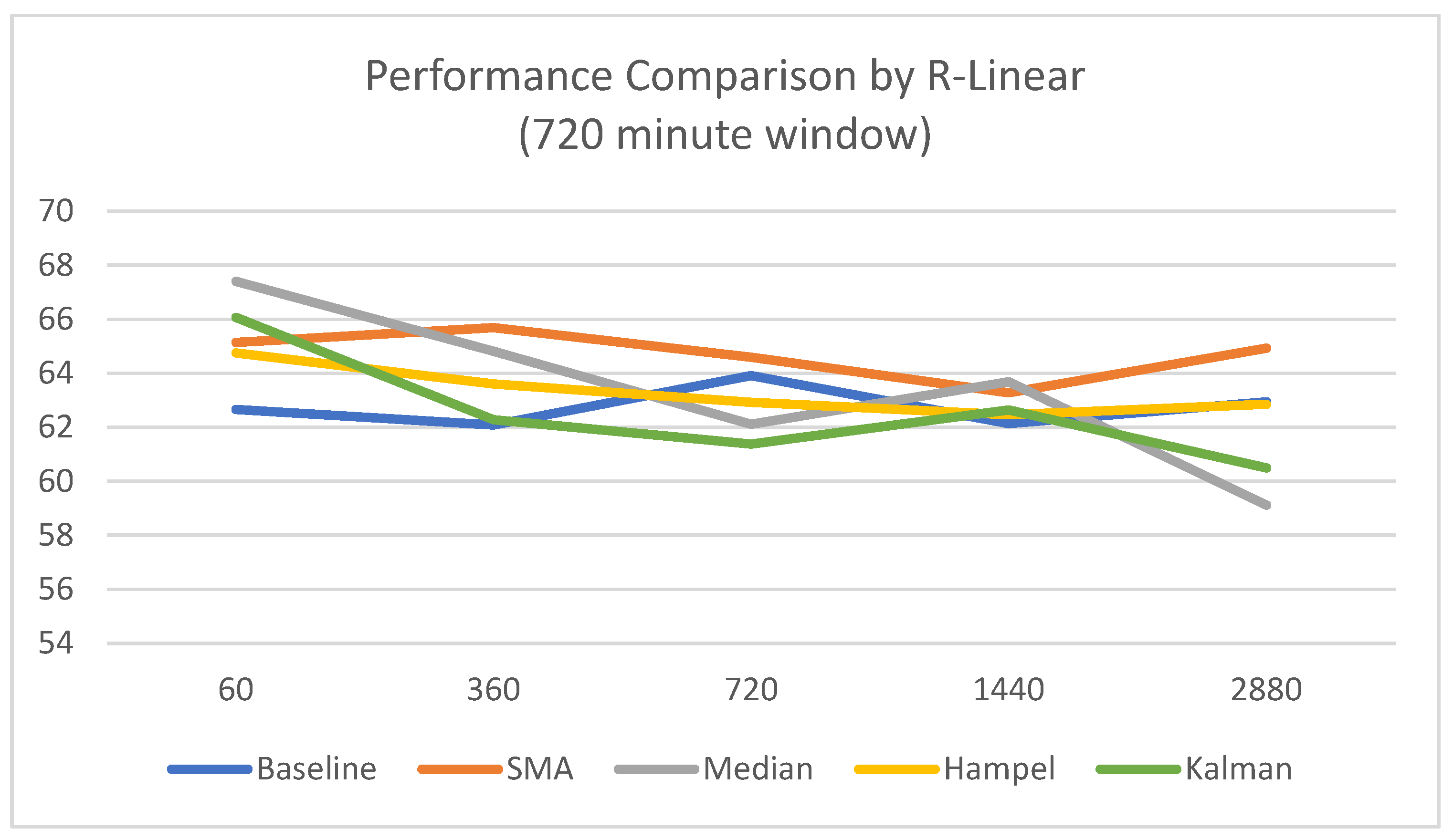
  • For the shortest prediction horizon (60 min offset), the Median filter recorded the highest mean accuracy (67.41%) but was also highly unstable, with a standard deviation of 11.08%.
  • The SMA filter once again proved to be the most robust technique, consistently achieving the best accuracy across most mid-to-long-term prediction horizons (360, 720, and 2880 min).
  • This confirms that even under inefficient input conditions, SMA is the superior technique for providing reliable and consistently high performance for long-term predictions with the R-Linear model.
For the shortest prediction horizon (60 min offset), the Median filter (67.41%) and Kalman filter (66.07%), which focus on outlier removal, recorded the highest mean accuracies, consistent with findings from the 360 min window experiment. However, in the case of the Median filter, its high standard deviation of 11.08% indicates that its predictive stability was very low, making it difficult to consider a practical technique.
In contrast, the SMA filter once again proved to be the most robust and reliable preprocessing technique, particularly under these inefficient input conditions. Although it did not achieve the top performance in the short-term prediction, it consistently yielded the best mean accuracy across most of the mid-to-long-term prediction horizons (360, 720, and 2880 min). This demonstrates that even when excessively long time-series data acts as noise, the SMA filter stably preserves the core trend of the data, thereby maximizing the long-term predictive performance of the R-Linear model.
Figure 5 illustrates the performance of the R-Linear model with an extended 720 min input window. Consistent with previous findings, using a longer time window resulted in an overall degradation of predictive accuracy. In this scenario, while the Median filter held a slight advantage at the shortest 60 min offset, the SMA filter demonstrated more robust and consistently superior performance across the majority of the mid-to-long-term prediction horizons. This result further reinforces that even under sub-optimal input conditions, the simple and stable nature of the SMA filter makes it the most effective and reliable pre-processing choice for the R-Linear model.

4.2. Results for Optimal Scenarios by Preprocessing Technique

Table 6 summarizes the optimal performance achieved by each preprocessing technique when paired with the two different model architectures, the Transformer and R-Linear. The optimal result across all experiments was achieved with the combination of the Transformer model and the SMA filter, using a 360 min window and a 60 min offset, which yielded an overall accuracy of 80.45%. This configuration, therefore, stands out as the most effective methodology identified in this study. A consistent trend was observed where the peak performance for most techniques was achieved under the short-term 360/60 scenario. This suggests that for this particular task, a shorter look-back window containing more recent historical data is more informative than an excessively long one.
Furthermore, a strong interaction between the model architecture and the optimal preprocessing filter was evident. While the complex Transformer model performed best with the SMA filter, the simple R-Linear model achieved its peak accuracy of 75.15% when combined with the Median filter—a technique that performed poorly with the Transformer. This highlights that the choice of the best preprocessing filter is not universal; rather, it is highly dependent on the intrinsic characteristics of the model architecture.
In conclusion, this study identifies the combination of a Transformer, an SMA filter, and a short-term 360/60 scenario as the optimal approach. Concurrently, it empirically demonstrates that the effectiveness of a preprocessing filter can vary dramatically depending on the model, reinforcing the importance of a data-centric approach that considers the interplay between data, preprocessing, and model selection.

5. Discussion

This study analyzed the impact of data preprocessing using a novel, high-density IIoT data from real-world industrial machine tools, which has not been previously reported in academic literature. This data, collected at one-minute intervals and comprising over 30 multivariate time-series, provided a foundation for exploring the complex characteristics of real industrial noise that are difficult to analyze with typical public datasets. Therefore, unlike existing studies that often assume ideal experimental conditions, this work has the distinct advantage of directly addressing the complexities and unique noise characteristics inherent in a real-world operational environment.
The experimental results show that the SMA filter achieved the highest overall performance in terms of accuracy while simultaneously demonstrating predictive stability, recording low standard deviations in most of the repeated experiments. This suggests that appropriate and efficient pre-processing still plays a crucial role in maximizing the performance of modern deep learning models. With the exception of SMA, most filters failed to outperform the baseline model and, in some cases, even degraded performance. Specifically, the Median and Hampel filters, which focus on outlier removal, not only showed low mean accuracy but also caused extreme predictive instability, as confirmed by their very high standard deviations, severely compromising the model’s reliability. This highlights a fundamental limitation of applying generic outlier removal techniques to complex industrial data. While these filters are designed to remove noise, prior research indicates that outliers can, in fact, be critical events for analysis [35]. In IoT systems, these can be meaningful operational events, distinct from simple sensor defects [36]. Therefore, we argue that the Hampel filter’s indiscriminate removal of these data points, without distinguishing between noise and important operational events, is the direct cause of the model’s degraded performance. Furthermore, the Kalman filter, a dynamic state estimator, was theoretically expected to provide significant performance improvements. However, the empirical results showed that while it achieved high mean accuracy in some short-term scenarios, it also exhibited high standard deviations. Moreover, its predictive accuracy was generally lower than that of the Baseline. This suggests that for this particular industrial dataset, the complex state-estimation mechanism of the Kalman filter may have over-fit to certain noise patterns, leading to unstable predictions. Conversely, the simple averaging approach of SMA proved to be a more robust strategy. This aligns with established principles of time-series preprocessing, where the goal of a smoothing technique is to reduce noise and short-term fluctuations to reveal the underlying pattern [37]. Our task of predicting power efficiency states depends on the longer-term trend of energy consumption, not short-term noise. As a classic smoothing method, the SMA filter is designed to attenuate irrelevant noise while preserving this essential trend [37]. Therefore, providing the model with a signal that highlights the core pattern serves as the theoretical basis for the superior performance of SMA in our experiments.
Furthermore, this study confirmed the impact of input data length, i.e., the window size, on model performance. The model generally achieved higher performance when using a 360 min window compared to a longer 720 min window, which implies that past data beyond a certain length can act as redundant noise.
These results offer important implications for practitioners in IIoT data analytics.
  • First, the SMA can be a more effective alternative to complex techniques. SMA provided an ideal balance between performance and stability by reducing unnecessary volatility while preserving key data trends.
  • Second, optimizing model performance requires not only selecting the right filter but also the appropriate length of the input data.
In conclusion, this study corroborates the principle that success in applied machine learning depends not on unreflective application of complex models or generic pipelines, but on a data-centric, nuanced approach that recognizes the unique characteristics of the problem domain.

6. Conclusions

This study empirically investigated the impact of various data pre-processing filters on the performance and stability of two contrasting deep learning architectures—a complex Transformer and a simple R-Linear model—for time-series classification in an IIoT environment. The research derived a clear conclusion: a data-centric approach, centered on applying a simple and computationally efficient filter like the SMA, was the most robust and effective strategy overall. This demonstrates that enhancing data quality is a critical prerequisite for maximizing the performance of modern deep learning models, regardless of their complexity.
The main findings and their implications can be summarized as follows. First, the optimal preprocessing technique varied dramatically depending on the model architecture. The complex Transformer model, with its attention mechanism, was able to capture the subtle characteristics of the data smoothed by the SMA filter to achieve its peak performance. In contrast, the R-Linear model, which is unable to leverage such complex characteristics to the same degree due to its simple linear structure, showed a complex pattern: it responded more favorably to data where outliers were effectively removed (as with the Median and Kalman filters) for short-term predictions, yet for long-term predictions, the SMA filter demonstrated superior performance. Second, the Kalman filter, despite its advanced design, was consistently outperformed by the much simpler SMA filter in terms of both peak performance and predictive stability. Third, this study confirmed the existence of an optimal context window. The 360 min window yielded superior results to the longer 720 min window, confirming that more historical data is not always better.
The results of this study underscore for Industrial AI practitioners the importance of a ‘data-centric’ optimization strategy over a purely model-centric one. Our findings show that significant performance gains can be achieved by thoughtfully selecting an appropriate, often simple, pre-processing technique and an optimal input data length, based on an understanding of the data’s inherent characteristics. Therefore, establishing a robust baseline with an interpretable and efficient method like SMA is a highly practical and effective approach. This study also underscores that predictive stability, validated through repeated experiments, is an indispensable requirement in industrial settings where reliability is paramount.
Finally, our findings suggest several promising directions for future research. First, to verify the generalizability of our findings—particularly the surprising effectiveness of the simple SMA filter—the experimental framework should be applied to diverse industrial datasets from other domains and to a wider range of deep learning architectures. Second, future work should focus on developing a systematic methodology for selecting the optimal preprocessing technique based on the characteristics of the time-series data and the chosen model architecture. Our results strongly indicate that there is no one-size-fits-all solution; for instance, while this study highlights the effectiveness of the SMA filter, its optimal parameters would likely need tuning for the specific noise characteristics of different industrial environments. Finally, future research should investigate hybrid approaches at both the preprocessing and model architecture levels. For instance, combining different models to leverage their unique strengths may be a promising avenue for enhancing predictive performance. Similarly, hybrid pre-processing techniques, which could combine the robust trend-smoothing of SMA with the specific short-term advantages of other filters (e.g., Median or Kalman), are expected to yield additional performance improvements by adapting to different prediction horizons.

Author Contributions

Conceptualization, S.-H.S., C.-S.S. and S.K.; methodology, S.-H.S., M.P. and S.K.; validation, S.-H.S. and M.P.; formal analysis, S.-H.S. and S.K.; investigation, C.-S.S.; data curation, S.-H.S. and C.-S.S.; writing—original draft preparation, S.-H.S. and C.-S.S.; writing—review and editing, S.-H.S., M.P. and S.K.; supervision, S.K.; project administration, S.K. These authors contributed equally to this work: S.-H.S. and C.-S.S. All authors have read and agreed to the published version of the manuscript.

Funding

This work was supported by the Technology Development Program of MSS [2420000355] in Republic of Korea.

Institutional Review Board Statement

Not applicable.

Informed Consent Statement

Not applicable.

Data Availability Statement

Data can be obtained at the following URL: https://github.com/sanghasung/ (accessed on15 October 25).

Acknowledgments

This research used datasets from ‘The Open AI Dataset Project (AI-Hub, S. Korea)’. All data information can be accessed through ‘AI-Hub (www.aihub.or.kr (accessed on 15 October 25))’.

Conflicts of Interest

Author Chang-Sung Seo was employed by the company SCT Co., Ltd. The remaining authors declare that the research was conducted in the absence of any commercial or financial relationships that could be construed as a potential conflict of interest.

References

  1. Kumar, A.; Selvakumar, V.; Lavanya, P.; Lakshmi, S.; Uma, S.; Naidu, K.B.; Srivastava, R. Optimizing Power Management in IoT Devices Using Machine Learning Techniques. J. Electr. Syst. 2024, 20, 2929–2940. [Google Scholar] [CrossRef]
  2. Ethan, A.; Karan, D. Energy-Efficient IoT Systems Using Machine Learning for Real-Time Analysis. Int. J. Mach. Learn. Res. Cybersecur. Artif. Intell. 2023, 14, 1307–1322. [Google Scholar]
  3. Solanki, A. Sensor Data Analysis for Enhanced Decision-Making in Industry. Int. J. Manag. IT Eng. 2024, 14, 1–14. [Google Scholar]
  4. Bilgili, M.; Arslan, N.; Şekertekin, A.; Yaşar, A. Application of long short-term memory (LSTM) neural network based on deeplearning for electricity energy consumption forecasting. Turk. J. Electr. Eng. Comput. Sci. 2022, 30, 140–157. [Google Scholar] [CrossRef]
  5. Kim, K.; Kim, D.K.; Noh, J.; Kim, M. Stable forecasting of environmental time series via long short term memory recurrent neural network. IEEE Access 2018, 6, 75216–75228. [Google Scholar] [CrossRef]
  6. Liu, Y.; Yu, W.; Rahayu, W.; Dillon, T. An evaluative study on IoT ecosystem for smart predictive maintenance (IoT-SPM) in manufacturing: Multiview requirements and data quality. IEEE Internet Things J. 2023, 10, 11160–11184. [Google Scholar] [CrossRef]
  7. Liu, Y.; Dillon, T.; Yu, W.; Rahayu, W.; Mostafa, F. Noise removal in the presence of significant anomalies for industrial IoT sensor data in manufacturing. IEEE Internet Things J. 2020, 7, 7084–7096. [Google Scholar] [CrossRef]
  8. Goknil, A.; Nguyen, P.; Sen, S.; Politaki, D.; Niavis, H.; Pedersen, K.J.; Suyuthi, A.; Anand, A.; Ziegenbein, A. A systematic review of data quality in CPS and IoT for industry 4.0. ACM Comput. Surv. 2023, 55, 1–38. [Google Scholar] [CrossRef]
  9. Patel, J.M.; Ramezankhani, M.; Deodhar, A.; Birru, D. State of Health Estimation of Batteries Using a Time-Informed Dynamic Sequence-Inverted Transformer. arXiv 2025, arXiv:2507.18320. [Google Scholar]
  10. Noura, N.; Boulon, L.; Jemeï, S. A review of battery state of health estimation methods: Hybrid electric vehicle challenges. World Electr. Veh. J. 2020, 11, 66. [Google Scholar] [CrossRef]
  11. Safavi, V.; Bazmohammadi, N.; Vasquez, J.C.; Guerrero, J.M. Battery state-of-health estimation: A step towards battery digital twins. Electronics 2024, 13, 587. [Google Scholar] [CrossRef]
  12. Oji, T.; Zhou, Y.; Ci, S.; Kang, F.; Chen, X.; Liu, X. Data-driven methods for battery soh estimation: Survey and a critical analysis. IEEE Access 2021, 9, 126903–126916. [Google Scholar] [CrossRef]
  13. Iurilli, P.; Brivio, C.; Carrillo, R.E.; Wood, V. Physics-based soh estimation for li-ion cells. Batteries 2022, 8, 204. [Google Scholar] [CrossRef]
  14. Jo, S.; Jung, S.; Roh, T. Battery state-of-health estimation using machine learning and preprocessing with relative state-of-charge. Energies 2021, 14, 7206. [Google Scholar] [CrossRef]
  15. Acurio, B.A.A.; Barragán, D.E.C.; Rodríguez, J.C.; Grijalva, F.; Pereira da Silva, L.C. Robust Data-Driven State of Health Estimation of Lithium-Ion Batteries Based on Reconstructed Signals. Energies 2025, 18, 2459. [Google Scholar] [CrossRef]
  16. Tang, X.; Liu, K.; Li, K.; Widanage, W.D.; Kendrick, E.; Gao, F. Recovering large-scale battery aging dataset with machine learning. Patterns 2021, 2, 100302. [Google Scholar] [CrossRef] [PubMed]
  17. Zhang, L.; Ji, T.; Yu, S.; Liu, G. Accurate prediction approach of SOH for lithium-ion batteries based on LSTM method. Batteries 2023, 9, 177. [Google Scholar] [CrossRef]
  18. Cui, S.; Joe, I. A dynamic spatial-temporal attention-based GRU model with healthy features for state-of-health estimation of lithium-ion batteries. IEEE Access 2021, 9, 27374–27388. [Google Scholar] [CrossRef]
  19. Cao, K.; Zhang, T.; Huang, J. Advanced hybrid LSTM-transformer architecture for real-time multi-task prediction in engineering systems. Sci. Rep. 2024, 14, 4890. [Google Scholar] [CrossRef]
  20. Wen, Q.; Zhou, T.; Zhang, C.; Chen, W.; Ma, Z.; Yan, J.; Sun, L. Transformers in time series: A survey. arXiv 2022, arXiv:2202.07125. [Google Scholar]
  21. Fatima, S.S.W.; Rahimi, A. A review of time-series forecasting algorithms for industrial manufacturing systems. Machines 2024, 12, 380. [Google Scholar] [CrossRef]
  22. Meng, F.; Wang, P.; Wang, J. Lithium-ion battery state of health estimation based on LSTM-transformer. In Proceedings of the 2024 IEEE 13th International Conference on Communication Systems and Network Technologies (CSNT), Jabalpur, India, 6–7 April 2024; pp. 1305–1310. [Google Scholar]
  23. Wang, M.; Sui, Z.; Zhang, L. State-of-Health Estimation of Lithium-Ion Batteries Based on EIS and CNN-Transformer Network. In Proceedings of the 2024 Global Reliability and Prognostics and Health Management Conference (PHM-Beijing), Beijing, China, 11–13 October 2024; pp. 1–7. [Google Scholar]
  24. Liu, Y.; Hu, T.; Zhang, H.; Wu, H.; Wang, S.; Ma, L.; Long, M. itransformer: Inverted transformers are effective for time series forecasting. arXiv 2023, arXiv:2310.06625. [Google Scholar]
  25. Eivazi, H.; Hebenbrock, A.; Ginster, R.; Blömeke, S.; Wittek, S.; Herrmann, C.; Spengler, S.T.; Turek, T.; Rausch, A. DiffBatt: A diffusion model for battery degradation prediction and synthesis. arXiv 2024, arXiv:2410.23893. [Google Scholar] [CrossRef]
  26. Zeng, A.; Chen, M.; Zhang, L.; Xu, Q. Are transformers effective for time series forecasting? In Proceedings of the AAAI Conference on Artificial Intelligence, Washington, DC, USA, 7–14 February 2023; Volume 37, pp. 11121–11128. [Google Scholar] [CrossRef]
  27. Li, Z.; Qi, S.; Li, Y.; Xu, Z. Revisiting long-term time series forecasting: An investigation on linear mapping. arXiv 2023, arXiv:2305.10721. [Google Scholar] [CrossRef]
  28. Johnston, F.R.; Boyland, J.E.; Meadows, M.; Shale, E. Some properties of a simple moving average when applied to forecasting a time series. J. Oper. Res. Soc. 1999, 50, 1267–1271. [Google Scholar] [CrossRef]
  29. Astola, J.; Neuvo, Y. Matched median filtering. IEEE Trans. Commun. 2002, 40, 722–729. [Google Scholar] [CrossRef]
  30. Liu, Y.; Wu, H.; Wang, J.; Long, M. Non-stationary transformers: Exploring the stationarity in time series forecasting. Adv. Neural Inf. Process. Syst. 2022, 35, 9881–9893. [Google Scholar]
  31. Yin, L.; Yang, R.; Gabbouj, M.; Neuvo, Y. Weighted median filters: A tutorial. IEEE Trans. Circuits Syst. II Analog. Digit. Signal Process. 1996, 43, 157–192. [Google Scholar] [CrossRef]
  32. Roos-Hoefgeest Toribio, M.; Garnung Menéndez, A.; Roos-Hoefgeest Toribio, S.; Álvarez García, I. A Novel Approach to Speed Up Hampel Filter for Outlier Detection. Sensors 2025, 25, 3319. [Google Scholar] [CrossRef] [PubMed]
  33. Hampel, F.R. The influence curve and its role in robust estimation. J. Am. Stat. Assoc. 1974, 69, 383–393. [Google Scholar] [CrossRef]
  34. Kalman, R.E. A new approach to linear filtering and prediction problems. J. Fluids Eng. 1960, 82, 35–45. [Google Scholar] [CrossRef]
  35. Blázquez-García, A.; Conde, A.; Mori, U.; Lozano, J.A. A review on outlier/anomaly detection in time series data. ACM Comput. Surv. (CSUR) 2021, 54, 1–33. [Google Scholar] [CrossRef]
  36. Yasaei, R.; Hernandez, F.; Faruque, M.A.A. IoT-CAD: Context-aware adaptive anomaly detection in IoT systems through sensor association. In Proceedings of the 39th International Conference on Computer-Aided Design, San Diego, CA, USA, 2–5 November 2020; pp. 1–9. [Google Scholar]
  37. Owen, A.; Doe, J. Forecasting Supply Chain Trends Using Time Series Analysis. 2024. Available online: https://www.researchgate.net/profile/Antony-Owen/publication/390300976_Forecasting_Supply_Chain_Trends_Using_Time_Series_Analysis/links/67e817c9e8041142a14f08d0/Forecasting-Supply-Chain-Trends-Using-Time-Series-Analysis.pdf (accessed on 16 October 2025).
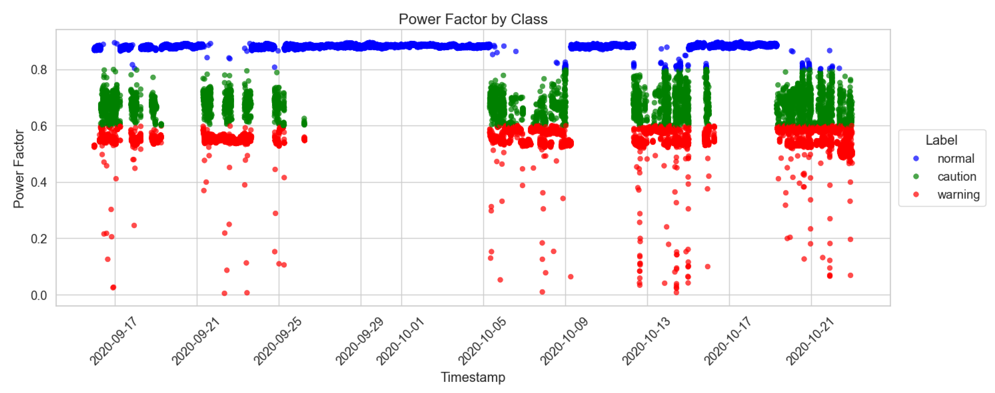
Figure 1. This plot displays the original power factor values collected from IIoT sensors, categorized by class. The data is categorized into three classes: Normal (blue), Caution (green), and Warning (red), as illustrated in the figure.
Applsci 15 11277 g001
Figure 2. Performance comparison of pre-processing techniques with the Transformer model using a 360 min input window.
Applsci 15 11277 g002
Figure 3. Performance comparison of pre-processing techniques with the R-Linear model using a 360 min input window.
Applsci 15 11277 g003
Figure 4. Performance comparison of pre-processing techniques with the Transformer model using a 720 min input window.
Applsci 15 11277 g004
Figure 5. Performance comparison of pre-processing techniques with the R-Linear model using a 720 min input window.
Applsci 15 11277 g005
Table 1. This table presents the distribution of data instances across the defined classes.
NormalCautionWarningTotal
Count31,25614,347767753,280
Percentage58.7%26.9%14.4%100.0%
Table 2. The table shows the prediction results of the Transformer model using a 360 min input window. The table presents the mean and standard deviation (Std.) for Accuracy and F1-Score, alongside the mean Training Time for each pre-processing scenario.
PreprocessingWindow/
Offset
Accuracy (%)Accuracy Std. (%)F1 Score (%)F1 Score Std. (%)Training Time (s)
Baseline360/6078.884.2659.586.30367.9
360/36072.123.9152.646.48367.8
360/72068.317.7149.887.18354.4
360/144065.253.4441.157.12341.4
360/288067.761.1145.932.71333.1
SMA360/6080.451.9460.392.18382.9
360/36072.278.1754.666.08373.9
360/72070.102.5953.272.45369.1
360/144068.803.0748.305.47381.2
360/288068.782.1649.923.04384.7
Median360/6065.1211.6039.1115.89347.4
360/36062.425.3932.7711.20348.3
360/72068.098.4649.3510.30343.0
360/144064.945.9538.3413.64334.5
360/288066.035.7744.277.32326.0
Hampel360/6069.967.7448.1311.47343.0
360/36064.538.2640.1511.38341.9
360/72068.142.8548.635.89336.2
360/144061.869.6440.447.66337.9
360/288066.542.2544.642.69336.9
Kalman360/6072.9610.6252.4511.67354.3
360/36069.325.0847.379.37353.3
360/72068.477.9449.718.53345.0
360/144067.753.3246.235.71346.5
360/288068.502.2447.652.96336.6
Table 3. The table shows the prediction results of the R-Linear model using a 360 min window.
PreprocessingWindow/
Offset
Accuracy (%)Accuracy Std. (%)F1 Score (%)F1 Score Std. (%)Training Time (s)
Baseline360/6072.255.8951.069.26145.3
360/36065.584.0041.758.07141.4
360/72063.831.9736.944.06141.1
360/144063.291.9535.154.30139.8
360/288061.563.0734.855.29136.3
SMA360/6072.619.1449.5013.04143.6
360/36064.418.3739.3810.76141.7
360/72062.5010.7137.887.89140.9
360/144063.662.2636.004.51138.7
360/288063.683.1038.675.45138.5
Median360/6075.1510.8555.0511.57145.9
360/36067.414.7246.386.49144.2
360/72064.603.3038.717.28142.3
360/144063.612.0235.184.04142.1
360/288062.713.1237.464.62138.2
Hampel360/6072.264.7151.417.50144.9
360/36061.958.9038.599.01141.8
360/72062.572.7133.985.94141.2
360/144062.732.0432.724.97139.1
360/288062.233.3233.077.20135.7
Kalman360/6074.796.3353.478.54191.2
360/36063.898.0739.529.84204.6
360/72059.998.4033.397.21198.7
360/144062.762.1734.415.34178.2
360/288061.077.1236.145.53161.8
Table 4. The table shows the prediction results of the Transformer model using a 720 min input window.
PreprocessingWindow/
Offset
Accuracy (%)Accuracy Std. (%)F1 Score (%)F1 Score Std. (%)Training Time (s)
Baseline720/6071.944.1152.566.60891.8
720/36069.233.6148.326.66866.0
720/72064.7712.0346.2810.25878.3
720/144062.299.7240.738.49867.4
720/288066.374.3746.315.36843.1
SMA720/6071.9813.7354.7510.22893.3
720/36070.917.8654.236.44886.6
720/72070.192.7752.134.50877.2
720/144067.103.1045.885.31854.9
720/288068.216.0548.645.40832.3
Median720/6067.1110.1244.8013.06894.8
720/36062.8610.7741.1310.98886.1
720/72057.2415.7139.6013.86875.6
720/144063.765.4540.1710.42856.8
720/288065.055.1140.9311.44830.9
Hampel720/6062.768.5738.4611.33881.6
720/36068.323.9045.607.85884.0
720/72065.407.8646.757.90877.6
720/144062.937.2240.007.40864.2
720/288068.043.7946.556.59834.5
Kalman720/6069.377.3545.3711.461007.6
720/36066.1010.7444.3511.08999.2
720/72061.7212.5541.8410.91969.2
720/144065.066.9643.696.35929.3
720/288066.485.8146.573.81869.5
Table 5. The table shows the prediction results of the R-Linear model using a 720 min input window.
PreprocessingWindow/
Offset
Accuracy (%)Accuracy Std. (%)F1 Score (%)F1 Score Std. (%)Training Time (s)
Baseline720/6062.6613.0640.0912.54232.9
720/36062.097.3434.909.59230.5
720/72063.922.9636.127.33225.4
720/144062.147.1035.596.05214.5
720/288062.942.6937.055.96206.9
SMA720/6065.146.9137.6813.31220.9
720/36065.694.9439.1110.51217.8
720/72064.592.4837.666.32216.3
720/144063.282.5333.595.86212.5
720/288064.938.7546.557.77206.7
Median720/6067.4111.0846.5511.00220.4
720/36064.818.6139.1911.28216.5
720/72062.116.9433.408.50216.6
720/144063.682.3236.005.66227.0
720/288059.1210.7733.597.79219.6
Hampel720/6064.767.5740.7510.12235.4
720/36063.603.5436.397.68235.2
720/72062.923.8635.228.15234.9
720/144062.472.4434.405.87227.5
720/288062.853.0635.847.26211.4
Kalman720/6066.079.2340.2412.48273.4
720/36062.287.0336.178.37276.7
720/72061.382.5530.277.44262.7
720/144062.642.4234.955.88255.9
720/288060.5010.6537.498.13248.5
Table 6. The table provides a comparative analysis of the optimal scenario for each preprocessing technique.
ModelPreprocessingConfiguration
(Window/Offset)
Accuracy
TransformerBaseline360/6078.88%
SMA360/6080.45%
Median360/72068.09%
Hampel360/6069.96%
Kalman360/6072.96%
R-LinearBaseline360/6072.25%
SMA360/6072.61%
Median360/6075.15%
Hampel360/6072.26%
Kalman360/6074.79%
Disclaimer/Publisher’s Note: The statements, opinions and data contained in all publications are solely those of the individual author(s) and contributor(s) and not of MDPI and/or the editor(s). MDPI and/or the editor(s) disclaim responsibility for any injury to people or property resulting from any ideas, methods, instructions or products referred to in the content.