Abstract
Rail transportation is one of the most environmentally friendly systems; however, it generates noise and vibrations in the vicinity of railway lines. Therefore, the operation of railways requires appropriate measurements to analyze interactions between rolling stock and railway infrastructure during service. This paper presents a novel railway monitoring system based on the Industrial Internet of Things (IIoT) sensor network concept, enabling the integration of functionalities such as synchronized motion, technical, and environmental measurements. The system features a flexible configuration regarding the number of monitored parameters and scalability in terms of the number of tracks being observed. Selected field studies are presented, leading to the optimal configuration of the measurement system, along with a discussion of key research findings. Signal analysis enables a comprehensive assessment of the impact of rail transport on the environment, particularly by identifying sources of environmental pollution such as vibrations and noise generated by rail vehicles. In this study, 932 units of passing trains (wagons, locomotives, and multiple unit sections) were identified. The average deviation of the distances between recorded axles (relative to the catalog data) was approximately 3.9 cm, with a maximum of 20 cm.
1. Introduction
Rail transport plays a crucial role in transportation systems worldwide, serving as one of the most environmentally friendly modes of moving people and goods. Despite its numerous advantages, railway operations pose several environmental and technical challenges, with noise and vibration emissions being of particular concern [1,2,3,4,5]. These factors can negatively impact both the quality of life for residents living near railway lines and the condition of the surrounding infrastructure [6,7,8,9,10,11,12,13]. The significance of these effects is growing as new urban areas continue to develop and existing ones expand, often in close proximity to railway corridors.
Research on noise and vibrations generated by rail vehicles encompasses the analysis of their generation mechanisms and methods for monitoring and mitigation [1,14,15]. In particular, studies [11,16,17,18,19,20], focus on the propagation of vibrations into soil structures and infrastructure elements near operational railway tracks [21,22]. The control and assessment of the impact of transport-induced vibrations on buildings are crucial aspects of analysis and research to ensure compliance with safety, comfort, and environmental protection standards [23].
In the literature, two main approaches to the analysis of these phenomena are distinguished: mobile and stationary measurement methods. Mobile measurements, conducted in moving vehicles, not only enable the recording of vibroacoustic parameters but also facilitate a comprehensive diagnosis of railway infrastructure [24,25]. Advanced technologies, such as inertial measurement units (IMU), global navigation satellite systems (GNSS), laser scanners, and high-speed cameras for image recording, are employed for this purpose [26,27]. The combination of these methods allows for the identification of track irregularities, analysis of track geometry, and assessment of defects in railway infrastructure. Mobile measurements with vibroacoustic characteristics are also employed in the analysis of passenger ride comfort [28,29,30,31] and the diagnosis of rolling stock [28,29,32,33,34,35].
The second approach involves conducting stationary measurements at specific locations [36]. These measurements aim to assess the impact of rail transport on both the environment and infrastructure located near railway lines [37,38]. In particular, areas with high population density, workplaces, residential neighborhoods, and regions of high ecological value are considered [39,40,41]. The results of these measurements are used to create acoustic maps and analyze long-term trends in noise and vibration emissions, which facilitates actions related to environmental protection and spatial planning [1,2,6,7,8,9,10,11,39,40,41,42,43,44].
The principles for conducting environmental studies are outlined in applicable standards and regulations [36,40,45,46,47,48,49,50] particularly those such as EN ISO 3095:2013, which specifies procedures for measuring noise emitted by railway vehicles, EN 15610:2019 [36,46], which defines methods for measuring the acoustic roughness of rails and wheels, and CNOSSOS-EU (Common Noise Assessment Methods in Europe) [51], a methodology for assessing environmental noise in EU countries. These standards ensure the consistency and comparability of results, which is crucial for evaluating the effectiveness of noise and vibration reduction strategies. They also serve as the basis for statistics such as noise maps [2,5,44]. The methodology for assessing vibroacoustic phenomena should be appropriately adapted to the characteristics of the measurement equipment, as well as the specifics of the terrain, environmental conditions, and other random factors affecting the measurement process [7,52,53,54,55].
In recent years, many countries have installed measurement stations along railway lines that record noise and other characteristic parameters related to train passage. Typically, the collected data includes the current time, duration of passage, speed, and length of the train. In Germany, 19 measurement stations have been installed [15]. In Switzerland, measurements have been conducted at six fixed locations since 2003 [56], enabling the transfer of significant results to the entire network of routes. In the Netherlands, five stations were installed in 2006 [42], with RFID (Radio Frequency Identification) tags used to identify trains. In Austria, a pilot station was set up in 2008, followed by two additional stations on main lines in 2009 and 2020 [57]. Two stations were installed in France in 2021 [50]. Noise monitoring stations perform continuous measurements and are equipped with measurement microphones, recording devices, and weather stations. Some of these stations have been expanded to include vehicle axle counters, accelerometers, and GSM data transmission systems.
The development of new monitoring and diagnostic methods is influenced not only by technical aspects but also by other factors. In the context of railways, planning plays a particularly important role, especially when aimed at minimizing potential disruptions to the timetable, a challenge that is becoming increasingly significant, given that in many countries, the number of passengers is expected to double by 2050 [58]. Equally important are the shortages of specialists, which highlight the need to develop measurement systems that work in conjunction with software to support both the measurement process and data processing [43,59].
The literature review indicates a growing demand for monitoring and diagnostic systems that combine multiple functionalities. As a result, solutions integrating the measurement of various physical quantities are increasingly being proposed. In the case of monitoring vibroacoustic phenomena, the measurement system is spatially distributed and can simultaneously cover multiple tracks. Proper assessment of phenomena associated with vehicle motion requires time synchronization of signals and knowledge of the relative positions of sensors in space. An important feature is also the system’s ability to be installed at any location. For this reason, software supporting the operator of the measurement system plays a crucial role, starting from the planning and installation stages of the measurement setup near the railway line.
The new aspects presented in this paper are as follows:
- The innovative measurement methodology extends the typical functionality of environmental studies related to monitoring vibrations and noise, enabling precise identification of a range of motion and technical parameters of railway vehicles;
- The integration of functionalities with measurement synchronization allows for effective and precise correlation of causes and identification of sources of vehicle impact on the environment;
- The monitoring concept employs an integrated multisensor measurement station with a sensor network and dedicated software;
- The monitoring station is characterized by flexibility in configuration regarding the number of measured parameters and scalability concerning the number of monitored tracks;
- The station is designed for easy installation on the railway line and simple configuration of parameters, allowing for convenient relocation of the measurement location.
For this purpose, a modular network structure was designed, characterized by the ability to configure individual modules, determine their locations, and scale the system within the studied area (adjusted to measurement needs). Additionally, an original IT system was developed to control the measurement process in such a way that measurements conducted over extended periods are automatic (hands-free), avoid the collection of excessive (irrelevant) data, and organize the information in a clear database structure. Data analysis will be performed in a dedicated IT system, which will manage all measurement data in post-processing, transforming it into defined indicators as well as motion, technical, and environmental parameters including motion, technical, and environmental parameters such as train type and speed, wheelset axle configuration, traffic intensity, vehicle type, noise and vibration metrics, and other parameters describing dynamic interactions. In this way, the measurement and IT system will function as an effective monitoring tool for assessing the impact of vehicles on the environment and railway infrastructure at the selected location. For these reasons, the measurement system represents an original approach. It integrates various measurement devices, automatically controls the triggering of measurements and data acquisition, and implements a set of proprietary algorithms during post-processing, enabling automatic vehicle identification and assessment of their environmental impact.
Section 2 presents the methodology for monitoring and the implementation of the sensor network on the railway line, highlighting its functional features, including the modular structure and scalability. Selected measurement results from tests conducted on the railway line are presented in Section 3. The results of the measurements and their processing using dedicated algorithms to identify individual parameters are illustrated and discussed. Section 4 discusses measurement results recorded during the passage of three representative trains: a modern electric multiple unit designed for high-speed operation (reaching 200 km/h), a conventional passenger train consisting of carriages pulled by an electric locomotive, and a freight train composed of wagons hauled by a freight locomotive. Finally, Section 5 provides a summary and conclusions, highlighting the potential of the measurement and analytical system developed by the authors in supporting railway infrastructure managers in monitoring and mitigating the impacts of railway traffic on the environment and the infrastructural surroundings of railway lines.
2. Materials and Methods
2.1. General Characteristics of the Monitoring System
Existing railway infrastructure and rolling stock monitoring systems rely on the installation of dedicated measurement devices at specific points along the railway lines, each with clearly defined purposes and parameters, such as monitoring the catenary network, current collectors, axle box temperatures, vehicle brakes, rail defects, and more [60,61,62,63]. Newer concepts involve the development of multisensor systems with data fusion and machine learning [64,65,66].
The spatial and specific nature of vibroacoustic phenomena in railways necessitates the development of an advanced system that integrates a range of measurement devices and sensors in the form of an IIoT (Industrial Internet of Things) sensor network [67,68]. The new integrated monitoring system proposed by the authors consists of two subsystems: the measurement subsystem and the IT subsystem. The measurement subsystem is designed as a Spatial Sensor Network (SSN), incorporating specialized measurement systems related to the passage of railway vehicles at monitored locations. The IT component primarily includes software for data acquisition, archiving, and analysis, as well as for evaluating indicators and presenting results. A key aspect of this measurement-IT system is its proper topology, which is related to the range of monitored parameters and the geolocation of SSN elements. Figure 1 shows the topology of a representative system. In the dedicated variant, the measurement system is designed to cover two tracks (in a double-track line) and engineering structures within the monitored area. An important feature of the system is its ability to be relocated to different monitoring areas along railway lines, as well as its scalability and ease of sensor reconfiguration.
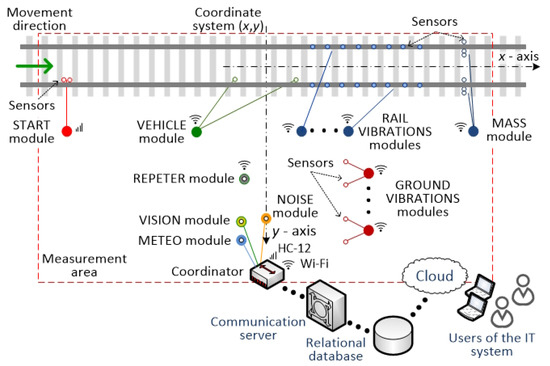
Figure 1.
Topology of the measurement system using a wireless sensor network, including examples of sensor types.
The selected parameters for monitoring were divided into three groups, which are as follows:
- Motion parameters: time of passage, vehicle speed, train composition characteristics (number of carriages, number of axles, train length), vehicle class/type, and vehicle traffic intensity at the studied location.
- Technical parameters: wheel mass and pressure on the rail track, wheel surface defects, and characteristics of running gear systems affecting the emitted vibrations and noise.
- Environmental parameters: noise emission around the railway line, vibration propagation in soil and engineering structures, and meteorological conditions.
To measure these parameters, specialized types of measurement modules were defined, each equipped with the appropriate sensors. The modules communicate with the master control unit, referred to as the Measurement System Coordinator (MSC), via wired or wireless connections.
The dedicated measurement modules include the following:
- START: This module triggers and ends the measurement cycle, initiated by a passing vehicle within the defined measurement zone. It also determines the direction of movement and estimates the approximate instantaneous speed of the train.
- NOISE: The main reference device for this module is a Class 1 sound level meter with specific measurement settings.
- METEO: A meteorological station that records weather parameters.
- VISION: This module is based on cameras that capture images of passing trains.
- VEHICLE: A module that detects the passage of consecutive vehicle wheels, enabling the calculation of the number and speed of vehicle axles and the distance between successive axles. In the later stage, it calculates train composition characteristics and traffic intensity.
- MASS: This module measures the wheel load exerted by the vehicle on the rail track, enabling the calculation of indicators related to the distribution of the vehicle’s mass and dynamic axle pressure on the railway track.
- RAIL VIBRATIONS: This module performs multipoint measurements of rail vibrations over a defined length of rail tracks, allowing for the assessment of the technical condition of the wheel tread surface, such as detecting wheel surface defects (e.g., flat spots).
- GROUND VIBRATIONS: This module performs multipoint vibration measurements from the railway surface to nearby engineering structures, allowing for the assessment of vibration propagation in the vicinity of the operational railway line.
- ACOUSTIC: A module for measuring the acoustic field in the immediate vicinity of the rail tracks.
- REPEATER: A module that extends the Wi-Fi communication range.
The monitoring system presented in Figure 1 consists, in part, of a wireless sensor network comprising measurement nodes, transmission nodes, and a coordinator [37,68]. This network requires specialized measurement sensors and appropriate module software. Each measurement sensor will be georeferenced by geodetic coordinates, enabling the unambiguous configuration of the sensor network components and their spatial identification at a specific measurement location. Depending on the adopted configuration, the measurement system can be implemented with either full or limited hardware coverage, on a single, double, or multi-track line.
In addition to the specific topology of the sensor network, the terrain and environmental conditions of the area where measurements are conducted are also crucial. To this end, geodetic measurements of the TSN topology around the railway line are performed. This is important due to the varying construction of the railway line along its length, including the trackbed, engineering structures, and other trackside devices [16,21,26].
2.2. Characteristics of Measurement Modules
The main environmental threats associated with the operation of railway lines are noise and vibration emissions. As a result, European normative acts and national regulations strictly define the requirements for measuring railway noise levels [36,50]. Meeting these conditions necessitates the measurement of noise, meteorological conditions, and vehicle motion parameters on the surveyed railway line. Instances in which the measured acoustic signal is deemed non-compliant with the requirements include:
- The simultaneous passage of two trains;
- The starting or braking of a railway vehicle on the test section;
- Measurements where background noise exceeds permissible threshold values [36] in relation to the measured sound level caused by the train’s passage;
- Measurements taken under meteorological conditions that do not comply with the guidelines applicable to the infrastructure manager.
In the presented project, commercially available devices with the appropriate class and parameters for environmental measurements were used, such as a Class 1 noise monitoring station in conjunction with a meteorological station. To assess the reliability of the acoustic signal, additional measurement modules, START and VEHICLE, were employed. The identification of the examined vehicle in the recorded acoustic signal is crucial [36], for which the VISION module was applied. For these devices, appropriate control functions have been developed to ensure their integration with MSC.
Figure 2 presents selected results from individual modules. Figure 2a shows acoustic events recorded by the NOISE module during the passage of railway vehicles. Figure 2b illustrates the wheel detection of an electric multiple unit (EN-57 EMU), presented as logical signals typical of the VEHICLE and START modules. Figure 2c displays the vertical acceleration of the track measured by a sensor of the RAIL VIBRATIONS module. Figure 2d shows the ground acceleration recorded 7.5 m from the railway track, along the transverse axis, using a sensor from the GROUND VIBRATIONS module. Both vibration traces (Figure 2c,d) correspond to the passage of a diesel multiple unit (SA-136 DMU) traveling at a speed of 24.4 m/s.
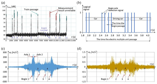
Figure 2.
Examples of signal traces from measurement modules: (a) NOISE module; (b) VEHICLE and START modules; (c) RAIL VIBRATIONS module; (d) GROUND VIBRATIONS module.
An important group of measurement modules consists of those specifically developed for the monitoring system, namely: START, VEHICLE, RAIL VIBRATIONS, GROUND VIBRATION, MASS, and ACOUSTIC. These modules operate by recording signals from various sensors, including accelerometers, microphones, inductive sensors, eddy current sensors, and others [38,69,70]. A universal structure and microcontroller system software were developed, enabling the registration of both digital signals to determine time events and analog quantities with varying numbers of measurement channels and sampling frequencies. The modules are based on popular Arduino Giga R1 WiFi evaluation kits, which communicate wirelessly with the MSC via a Wi-Fi network. This kit is equipped with a dual-core 32-bit STM32H747XI microcontroller, featuring ARM Cortex-M7 and Cortex-M4 cores. Due to time constraints, measurement results during vehicle passage are saved on an SD memory card. The general block diagram (and its technical implementation) of the microcontroller part of the module is shown in Figure 3. Depending on the module type, they vary in the interface used to couple the sensors with the microcontroller. It should be emphasized that the system is at the prototype stage; therefore, the construction of some devices was realized using evaluation kits. The Arduino Giga R1 WiFi platform was used during the prototyping phase of the system. This platform was chosen due to its relatively high signal processing capabilities, extensive supporting software, easy availability, and low implementation costs. During the measurement campaigns, the platform proved its suitability for this type of application and its compliance with the adopted design assumptions.
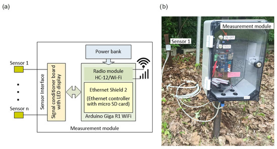
Figure 3.
General hardware architecture of the measurement module based on the Arduino Giga R1 board: (a) general block diagram, (b) prototype measurement unit (sensor and module).
The START module is equipped with specific firmware and a communication interface. It detects the wheel edge of the vehicle based on the signal from the wheel detector mounted on the inner side of the rail track. Two inductive sensors are placed at a fixed distance of several dozen centimeters from each other, allowing for:
- Detection of the event when the first wheelset axle of the train passes over the detector;
- Determination of the direction of train motion;
- Approximate estimation of the train’s speed;
- Detection of the event marking the end of the train’s passage, related to the movement of the last axle over the wheel detector.
Due to the relatively short time intervals between detecting the wheels of a train during high-speed passages and the need for real-time analysis, it was decided to use the microcontroller’s hardware counter. This counter works with registers that store its value when defined signal edges (input capture) from the wheel detector occur. This enables software processing of the input capture results and synchronization of calculations with the detection of the train’s wheels.
The VEHICLE module uses the same detectors as the START module, but they are installed at a greater distance from each other, several meters apart. Analyzing the signals from the sensors allows for, among other things:
- Counting the number of train axles, determining the train length, and analyzing its composition (including extracting the axles of bogies and wagons to determine the vehicle geometry);
- Calculating the train’s speed (both the instantaneous speed of each axle individually and the average speed).
The signals from the sensors are binary; however, to standardize the operation of the measurement modules (using the same embedded software), the VEHICLE module samples the signals as analog signals, with discretization occurring during result processing. The two signals must be measured at a frequency of 20 kHz and an amplitude of approximately 1000 m/s2. Figure 2b shows a fragment of the signal waveform from the wheel detectors during a train pass.
The primary task of the rail vibration module is to detect wheel defects that may cause excessive noise. Specifically, this concerns so-called ‘flat spots’ on the wheel (damage to the wheel’s tread surface), which can generate large impact loads on the rail. The RAIL VIBRATIONS module uses a set of single-axis MEMS accelerometers mounted on the rail base using magnetic holders. In the measurement system, the accelerometer sets are installed on each rail track, between successive ties, over a length of approximately 4 m, enabling the detection of point defects on the entire circumference of the vehicle’s wheels—requiring multiple measurement modules. Each sensor generates two signals: an acceleration signal in the vertical Z axis (analog) and a signal indicating range exceedance (digital). For each sensor, the signal must be measured at a frequency of at least 6 kHz. Figure 2c shows an example of the vertical rail vibration acceleration waveform during the passage of a diesel multiple unit (DMU) of the SA-136 type, with a clear correlation between acceleration impulses and the presence of the vehicle’s axles.
Mechanical vibrations are generated at the contact point between the vehicle’s wheels and the rail, propagating through the track structure and subgrade to the ground, affecting the surrounding environment of the railway line, including existing buildings [17,39]. To determine the magnitude of these vibrations, the GROUND VIBRATIONS module is used, which is constructed similarly to the RAIL VIBRATIONS module, but is equipped with three-axis MEMS accelerometers. The number and location of the sensors are not strictly defined and depend on the infrastructure surrounding the measurement zone. For each sensor, analog signals must be measured at a frequency of about 2 kHz and amplitudes of up to 10 m/s2. Figure 2d shows example ground vibrations in the transverse direction to the track during the passage of a diesel multiple unit (DMU). A clear correlation between the ground vibrations and rail vibrations (Figure 2c) is visible, while ground vibrations along the track axis are significantly attenuated. In the final processing (post-processing), third-octave vibration analysis indicators can be obtained [4].
The issue of wheel load pressures on rails is directly related to the vehicle’s structural mass and the weight of its cargo. The problem of determining a vehicle’s weight in motion is widely discussed in the literature under the term WIM (Weight in Motion) [70,71]. The method used by the authors allows for estimating the weight applied to the passing axles by measuring signals from two pressure sensors placed symmetrically on both sides of the rail track. Additionally, a signal from a track deflection sensor is recorded. The MASS module uses a set of three eddy current sensors with amplifiers for each rail track. Each sensor requires the measurement of one analog signal with a frequency of at least 1 kHz. The measurement system needs proper calibration. For weight estimation and the detection of abnormal conditions, it is sufficient to scale the data for all train axles, taking into account the known pressures of reference vehicles.
The optional ACOUSTIC module uses a set of microphones to measure the acoustic field in the immediate vicinity of the track during the passage of a train. The arrangement of the eight microphones is similar to that of the sensors in the RAIL VIBRATIONS modules, but positioned at a certain distance from the track. Analyzing the signals from the microphones allows, among other things, for the detection of bogies and axles of the vehicles. Each microphone generates an analog signal, which must be measured at a frequency of 44–48 kHz, necessitating the use of multiple modules.
2.3. Configuration and Control of the Measurement Process
The devices connected to the TSN are controlled by the MSC, a universal industrial computer with dedicated software developed specifically for this project. The main tasks of the MSC include managing the measurement process, controlling the start and end of measurements, as well as acquiring and temporarily archiving data from individual modules. The key functions of the MSC are as follows:
- Configuring the measurement session (determining the number of measured tracks and assigning measurement modules to specific tracks);
- Configuring measurement modules (setting data transmission parameters, sensor positions, sampling frequency, number of channels, etc.);
- Establishing data transmission with measurement modules and monitoring their status;
- Monitoring events and controlling the measurement process;
- Receiving measurement data files from modules, performing preliminary processing, and archiving them in the required text file formats.
In Figure 4, the main screen of the MSC control program is shown. The primary task of the user after launching the program is to configure the measurement session and select the appropriate measurement modules. After successful configuration, the program operates fully automatically, responding to messages sent by the modules connected to the TSN. The system’s operational status is continuously displayed on the screen, allowing the user to monitor connection quality and transmission errors from individual modules. Additionally, the program offers manual control of the measurement process, including the ability to check the status of the modules and start or stop measurements.
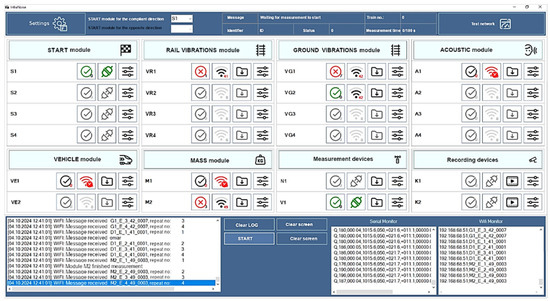
Figure 4.
User interface of the MSC software, with highlighted module windows and measurement status control panels.
The essence of the MSC operation lies in the automatic control of modules and measurement devices connected to the TSN. Figure 5 illustrates the basic sequence of MSC operation, using the example of the installation of a START module and the passage of a train along the railway line. The MSC program responds to messages sent from the START module according to developed algorithms, sending appropriate commands to the wirelessly connected measurement modules. The system supports two measurement control commands (BEGIN and END) as well as a status query command (STATUS). The program verifies the validity of the messages by analyzing their length and structure. Any errors that occur are signaled and logged in the program log. The status of the measurement modules is checked cyclically every minute when no measurement is in progress. The measurement begins after receiving the BEGIN command from the START module, which signals the train’s passage in the direction consistent with the railway mileage. At this point, a new measurement identifier is generated, which is then sent to the measurement modules along with the command to begin measurements. The measurement time is calculated based on the train’s speed and the location of the START module. The vehicle’s speed is sent along with the END command from the START module after the last wheelset of the train is detected. The measurement ends either when the measurement time is exceeded or when the user presses the STOP button. Once the measurement is completed, the measurement metrics are recorded, including information about the measurement, the collected data, and the current system configuration.
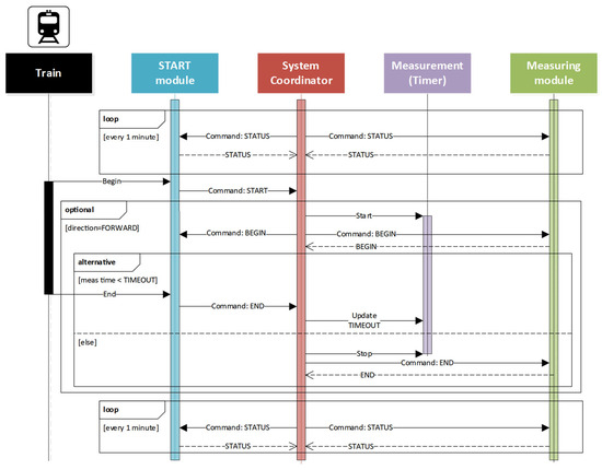
Figure 5.
Basic operational sequence of the MSC.
2.4. Data Processing and Reporting on Traffic, Technical, and Environmental Parameters—Data Analysis Methodology
The measurement system continuously collects data; however, its registration is not continuous, as this would generate too large an amount of data. Instead, the process is controlled by the MSC—individual measurement modules are activated only for a specified period, correlated with the passage of the vehicle through the measurement area. The MSC organizes the data in a defined folder structure, where measurement files are wirelessly transmitted from the modules. The data is then converted from binary format to a predefined text format containing sampled voltage signals. The prepared data is further analyzed during post-processing by the algorithms of the system’s IT component.
In Section 2.4.1, Section 2.4.2 and Section 2.4.3, example analytical algorithms that operate on measurement data for three selected modules are presented.
2.4.1. Processing of Acoustic Signals for Measurement Purposes
Figure 6 presents an example algorithm for processing an acoustic signal recorded by the NOISE module, incorporating data from the METEO module, two START modules (S1, S2), and the VEHICLE module. This allows for the assessment of the measurement’s compliance with the standard. This example refers to a double-track line with established directions of motion, as detected by S1 and S2.
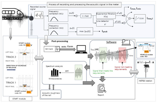
Figure 6.
Example algorithm for processing the acoustic signals.
The functionality of the NOISE module, in accordance with standards, is based on the measurement time. To meet the formal requirements, this module must record acoustic signals for at least 24 h, starting at 6:00 AM. Continuous measurement is planned, which requires defining time windows during the passage of specific types of rail vehicles. To determine the presence of a train on the track and to mark the start and end times of the acoustic measurement window, START modules installed on both tracks are used. Detection of vehicle presence on both tracks results in a measurement that is non-compliant with the standard [36].
Another module connected to the NOISE module is the VISION module. During post-processing, the VISION and VEHICLE modules provide information about the type of vehicle for which the measurement was taken, allowing for the classification of the acoustic signal measurement time window according to specific rail vehicle types [51].
An essential module for determining noise measurement compliance with standards is the METEO module [36], which provides meteorological data (e.g., temperature, atmospheric pressure, humidity, wind speed, and direction) sampled every second during the acoustic event. These modules supply data that, during post-processing (Software block), helps determine whether the recorded signal is compliant with the standard (green window) or non-compliant (red window)—as shown in Figure 6.
Standard [36] requires the use of a Class 1 sound level meter. This means that the meter must meet accuracy requirements of ±1 dB under environmental conditions (across a wide temperature range from −10 °C to +50 °C) and across a wide frequency range from approximately 16 Hz to 16 kHz, with a dynamic range (linearity) of at least 60 dB. The meter selected for the application (Svantek SV 307A [72] also features A, C, and Z weighting filters, as well as Fast, Slow, and Impulse response times in accordance with standard [53].
The meteorological station integrated into the system is the GMX600 Compact Weather Station, with specifications provided in the datasheet available at [73]. The VISION module is based on two cameras Basler ace acA2040-90umNIR [74].
2.4.2. Processing of Vibration Signals in the Vicinity of the Railway Line
Mechanical vibrations are generated at the wheel–rail contact area and propagate through the railway track structure to the ground, affecting the surrounding area of the railway line, including existing buildings. The specific speed and axle spacing of the wagons cause the passing train to be a source of cyclic excitation with a set frequency, which can lead to adverse escalation of interactions. Vibration measurements are carried out by the GROUND VIBRATION modules.
Appropriate signal processing algorithms allow for the determination of amplitude–frequency characteristics of vibrations, which are used, among others, in assessing their impact on the environment and the level of harmfulness.
Signals processing and the assessment of their impact on the environment is contained in five blocks:
- One-third Octave Band for buildings (1/3 OBB);
- One-third Octave Band for people (1/3 OBP);
- Signal Centering (SC);
- Signal Filtering (SF);
- Spectral Analysis (SA).
The analysis of the impact of vibrations on buildings (Block 1/3 OBB) is carried out using the Dynamic Influence Scales (DIS) method. Buildings are classified into one of two scales: DIS-I or DIS-II, depending on the number of floors and the dimensions of the horizontal projection. In each DIS scale, five damage zones (I, II, III, IV, V) are distinguished, separated by four boundary lines (A, B, C, D). The diagnostic methodology is based on in situ measurements of the building’s accelerations under real operational conditions (in situ testing). Vibrations are measured at the rigid nodes of the structure, at the junctions of main structural walls in the foundation or ground level. The horizontal directions of vibration (x, y) are verified.
The basic algorithm involves the one-third octave analysis of the recorded signals. Each signal is filtered into successive one-third octave bands within the central frequency range of 1–100 Hz. For each band, the extreme vibration amplitude is determined. The results, in the form of pairs of the central frequency of the one-third octave band and extreme acceleration amplitude, are plotted on the corresponding DIS scale. Comparing the results from the measurements (one-third octave analysis) with the normative values (DIS scale) allows for determining the harmfulness level of vibration and assessing the safety of the diagnosed building.
The analysis of the impact of vibrations on people staying in buildings (Block 1/3OBP) is carried out based on acceleration measurements of floors, in the places, where people stay during the day and night. Measurements are made in three directions: vertical (z) and horizontal (x, y). The evaluation is performed based on the root mean square values (RMS) of the filtered signals in third-octave bands within the frequency range of 1–80 Hz. The RMS metric is commonly used in signal analysis, as it quantifies the signal energy [20]. For discrete signals with a zero mean value, the RMS value of the sequence of N samples (where N corresponds to the time of vibration) is calculated as follows:
where
—the root mean square (RMS) value of the measured signal in the i-th third-octave band with a central frequency ;
—the k-th sample of the signal;
—the total number of samples.
The results for each third-octave band can be compared with the maximum permissible values [75], which refers to the vibration comfort limit for a given direction of vibrations.
where
—the value corresponding to the threshold of vibration perception by humans in the i-th third-octave band with the central frequency .
—a coefficient dependent on the building’s purpose (residential buildings, public utility buildings, hospitals, workspaces, etc.), the time of occurrence of vibrations (day, night), and the duration of vibrations (short-term vibrations, long-term vibrations). The vibration comfort limits can be determined for successive values of (n = 1, 1.4, 2, 4, 8, 16, 32, 64, 128).
During measurements, unexpected situations may occur, causing sudden or gradual deviations from the initial sensor axis position (e.g., impacts, settlement, tilts, temperature changes, or strong wind gusts). These effects manifest in the recorded signals as permanent axis shifts (i.e., DC offsets), jumps, or linear and nonlinear drifts. These effects must be eliminated before the signals can be further used for diagnostics. This is achieved at the initial stage of processing through the signal centering algorithm (SC). The operation of the algorithm is illustrated in Figure 7, using real measurement signals containing errors in the form of a step offset (Figure 7a) and a linearly increasing drift (Figure 7b). On the right-hand side, the signals where these effects have been effectively reduced by the centering algorithm are shown (Figure 7c,d).
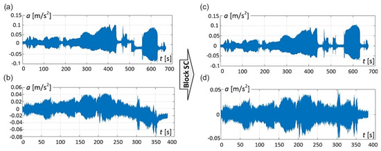
Figure 7.
Signal centering in the data processing from the GROUND VIBRATIONS module: (a) signal with a step offset, (b) signal with a linearly increasing drift, (c,d) signals centered using the SC algorithm.
The spectral analysis block (SA) allows performing a discrete Fourier transform (DFT), calculating the power spectral density (PSD) and the averaged normalized power spectral density (ANPSD) functions. The Power Spectral Density (PSD) and Averaged Normalized Power Spectral Density (ANPSD) metrics [76] are commonly used in vibration analysis of structures. The PSD describes the distribution of vibration energy of the k-th signal as a function of frequency, whereas the ANPSD is computed for the entire set of measured signals and represents the frequency components’ power shared across all measurements. This approach facilitates the identification and comparison of dominant frequency components present in the complete measurement dataset. The PSD of the k-th signal is defined as the dot product of the Fourier transform of this signal and its complex conjugate :
where
—i-th ordinate of the Power Spectral Density (PSD) of the k-th vibration signal corresponding to the i-th frequency ;
—the i-th value of the Discrete Fourier Transform (DFT) of the k-th signal at the i-th frequency ;
—the i-th frequency bin of the DFT of the k-th signal;
—sampling interval;
—the complex conjugation of .
The ANPSD is calculated for a set of K’s measured signals as follows:
where
—the i-th value of the Averaged Normalized Power Spectral Density (ANPSD) computed over a set of signals, corresponding to the i-th frequency ;
—the i-th value of the Power Spectral Density (PSD) for the k-th vibration signal at the i-th frequency as defined in Equation (3);
—the number of samples of the k-th signal.
The SF block allows for signal filtration within a selected frequency range (f1, f2). The module offers the choice between two types of filters: Butterworth filter and rectangular window filter. Figure 8 demonstrates the results of the filtration algorithm (SF) and the spectral analysis algorithm (SA) on the example of measured acceleration signals on building during the passage of the InterCity train. The filtration was carried out in the one-third octave band with a central frequency of f0 = 50.8 Hz. Figure 8a–c present the results as raw data, whereas Figure 8d–f show the signals after filtering.
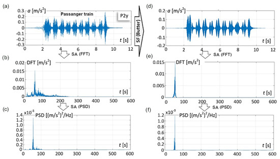
Figure 8.
Filtration and DFT and PSD of signals in the data processing from the GROUND VIBRATIONS module: (a) raw signal, (b,c) transforms of the raw signal, (d) filtered signal, (e,f) transforms of the filtered signal.
The above procedures for processing measurement data represent a typical approach to post-processing vibration acceleration signals. A key issue was the selection of sensors that would meet contemporary recording standards, i.e., appropriate bit resolution, frequency range, and amplitude range. The authors decided to use relatively inexpensive and readily available sensors that, during the prototyping phase, would satisfy accuracy requirements. The complete sensor with an evaluation board (EVAL-ADXL354BZ, [75]) was subjected to comparative tests with a commercial sensor, the 4312M3-002 from STRAINSENS [76]. The tests were conducted in the laboratory by exposing the sensors to vibrations generated by a shaker. Comparative analysis demonstrated the suitability of the selected setup for measuring accelerations on building structures.
2.4.3. Determining the Rail Vehicle Composition Characteristics
The determination of the vehicle composition characteristics is based on data recorded by the VEHICLE module. The complete sensor with an evaluation board (EVAL-ADXL354BZ [77], the 4312M3-002 from STRAINSENS [78].This module consists of two inductive sensors IIS284 IIK3030-BPKG/K1/V4A/US-104 [79] placed along the rail track, which detect the edge of the vehicle’s wheels and record this as logical signals in the microcontroller’s memory. This operation is similar to the wheel detectors used in railway traffic control systems. The sensors are positioned at a known distance D (several meters), which is determined during the installation of the setup. The registered wheel detection times allow for the calculation of the instantaneous speed of each axle of the vehicle. This speed is then used to calculate the distance between axles La and to determine the geometric dimensions of the rail vehicle composition. The conducted research demonstrated 100% effectiveness in axle identification, indicating that the selected sensors possess sufficient performance characteristics.
Sample data recorded by the VEHICLE module are shown in Figure 9. The selected segment corresponds to the impulses generated by the wheels of a single wagon’s bogie. Based on the signal analysis, several indicators characterizing the vehicle within the measurement area are determined. These include the number of axles, the number of wagons, speed, and rail vehicle length. Data from the VEHICLE module are also used to determine traffic intensity. From a metrological point of view, determining the distance La between vehicle axles is particularly important. These distances refer to the spacing between axles within a bogie, between axles in adjacent bogies within a locomotive or the same wagon, or between wagons, or between a wagon and a locomotive. Determining these distances allows for the calculation of the length and also enables the classification of whether it is a traction unit or wagons pulled by a locomotive, as well as determining the number of wagons. The algorithms used to calculate these indicators are based on the fact that axle spacing within bogies is a characteristic measurement, precisely defined for a given type of locomotive or wagon.
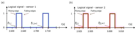
Figure 9.
Sample data plot recorded by the VEHICLE module: (a) for sensor 1; (b) for sensor 2.
To determine the distance between axles and the vehicle speed, it is necessary to know the times characterizing the registered impulses. The rising or falling edges (Figure 9) or the center time of the impulse can be used as reference points. In the presented analysis, the rising times were adopted.
The algorithm utilizes tables of time stamps identifying the passage moments of wheel axles over two sensors installed on the track, spaced at a precisely defined distance . Since the velocities of consecutive axles along the section between the sensors may slightly differ, the average of time intervals was used to determine the axle spacing . As a result, Equation (5) was obtained, defining the distance between consecutive axles (axle i and axle i + 1). In the implemented algorithm, axles are indexed and stored in table form:
where
—distance between subsequent vehicle axles;
—number of axels;
—distance between the sensors of the VEHICLE module;
—time stamps returned by sensor 1;
—time stamps returned by sensor 2;
—sensor index (n = 1, 2).
The measurement of the distance between axles is an indirect measurement, dependent on the sampling period of the analog–digital converter, the distance between sensors, and the vehicle speed . The difference in the values of the distance resulting from the chosen sampling period , is 0.2% for 0 μs and a vehicle speed of 200 km/h. For the nominal axle spacing in the bogie of 2500 mm, this corresponds to 5.5 mm. The measurement uncertainty of the distance , resulting from factors such as the calibration uncertainty of the measuring tape (1 mm), causes a difference in the calculated distance of approximately 0.02%. Therefore, both of these factors can be considered to have an insignificant impact on the obtained results. Determining the distance requires indirectly determining the vehicle speed . Speed measurement can be performed using an independent device, or data from the VEHICLE module sensors can be used for this purpose, with the Equation (6). This approach (measuring the passage time of axles through sensors spaced by allowed obtaining relatively accurate results for the instantaneous velocities of individual axles.
where
—the instantaneous velocity of the i-th axis;
—time stamps of the passage of the i-th vehicle axle over sensors 1 and 2.
It is crucial to consider the possibility of changes in the vehicle’s instantaneous speed as it passes through the measurement area (see Figure 1). For example, for a freight train consisting of a locomotive pulling 22 wagons, a speed difference of 13 km/h was recorded between the locomotive and the last wagon. Assuming an average speed instead of the instantaneous speed for each axle results in a difference of 8.9%. This corresponds to 150 mm for an axle spacing of 1800 mm in the wagon’s bogie. For the entire vehicle, this leads to a discrepancy of 53 m for a train length of 598 m. This example highlights the importance of determining the vehicle’s instantaneous speed.
The analysis also considered the results when the times corresponding to the centers of the impulses for each vehicle wheel were used. The obtained results were similar to those presented, but with smaller differences in .
2.4.4. Train Type Identification
The train identification algorithm consists of two main stages: acquisition of measurement data and matching the axle sequence to a database of vehicle patterns. A block diagram of the algorithm is shown in Figure 10.
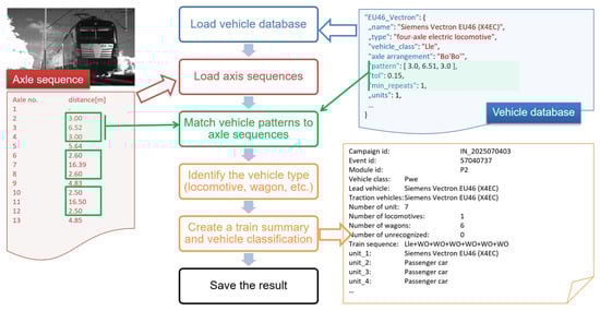
Figure 10.
Block diagram of the train type identification algorithm.
In the first stage, signals from the VEHICLE module sensors are analyzed to detect impulses corresponding to the moments, when vehicle axles pass over the sensors. For each sensor pair, the time difference is calculated, which is then used to determine the vehicle speed and the distances between successive axles. The resulting sequence of axle distances describes the geometric structure of the vehicle.
In the second stage, this structure is matched against a database containing characteristic axle layouts for locomotives, multiple units, and wagons. The vehicle identification algorithm is based on two main functions: match_pattern() and find_vehicles() (Figure 10).
The match_pattern() function evaluates whether a fragment of the axle distance sequence corresponds to a vehicle pattern. For each axle, the deviation from the pattern is calculated; if all deviations are within the allowed tolerance, the match is considered complete. The function also handles repeated segments, e.g., multiple wagons of the same type.
The find_vehicles() function searches through the entire measurement sequence, iteratively matching fragments to the pattern database. Matched vehicles are recorded along with their position and type.
Locomotives are characterized by unique axle spacings; however, this data is less readily available. Multiple units can be easily identified due to the repetitive nature of their sections and the long sequence of axles. Wagons are the least distinguishable because of the large number of types and similar axle spacings.
The effectiveness of the algorithm depends both on the quality of the measurement data (accuracy of axle and speed detection) and on the detail and representativeness of the pattern database.
This approach enabled complete and reliable identification of all analyzed types of railway vehicles across measurement campaigns on railway lines. Analysis of the results showed that the pattern matching accuracy for individual vehicle classes ranged from single millimeters to a few centimeters. For locomotives (63 vehicles in 12 types to identify), the maximum deviation did not exceed 6 cm, with an average matching error of 1.5 cm. For multiple units (8 types, 41 vehicles), these values were 4.1 cm and 2.1 cm, respectively; while for wagons (12 types, 828 vehicles), they were 20 cm and 7.5 cm.
The developed system enables automatic recognition of train type and structure, as well as the generation of statistics on pattern matching and measurement quality.
2.5. Field Test
To verify the concept of a monitoring station for motion, technical, and environmental parameters near a railway line, field tests were conducted. A set of measurement modules was selected, specifically designed to measure noise and vibration emissions, as well as to determine the motion parameters of vehicles. Measurements were carried out at locations meeting the requirements for environmental studies—in particular, those related to the influence of terrain topography and potential obstacles such as vegetation or engineering structures that could affect the noise emission process [36]. A section of the railway line arranged as a long straight track was selected, ensuring stable sound propagation conditions and convenient access to the track. It should be emphasized, however, that both the developed measurement methodology and the system’s hardware and software functionalities do not restrict the choice of locations solely to straight track sections. Although, at this stage, the measurements were conducted under conditions meeting the basic requirements for environmental studies, the authors plan to carry out experiments in varied field conditions in the future, pursuing additional objectives such as analyzing the influence of track geometry and its surroundings on vibration and noise emissions.
In addition to the specific topology of the SSN, the terrain and environmental conditions of the measurement area are of critical importance. To this end, geodetic surveys of the SSN topology in the vicinity of the railway line were carried out. This is particularly relevant due to variations in railway construction along its length, including the trackbed, engineering structures, and other trackside devices. For instance, near railway-road crossings or adjacent to bridge structures, local fluctuations in sound and vibration levels emitted into the environment can be observed.
Alongside these environmental considerations, each module and device is assigned a unique identification code, ensuring unambiguous identification of every component within the SSN. Furthermore, georeferencing points are established and documented using geodetic coordinates. This approach facilitates the precise configuration of the sensor network components and their spatial localization at specific measurement sites. The spatial configuration of the SSN (active sensors and their placements), along with photogrammetric documentation, is recorded in the MSC. Depending on the selected configuration, the measurement system can be deployed with either a full or limited hardware scope, on single-track, double-track, or multi-track railway lines.
Two measurement campaigns were conducted at distinct locations. The campaigns differed substantially both in terms of the number of sensors within individual measurement modules and in the approach to measurement control. The second campaign built upon the technical and technological advancements achieved during the first. The measurement methodology under development has now reached a stage of full automation, encompassing not only the management of the SSN but also the archiving of measurement signals and the preliminary processing of collected data.
Figure 11 presents low-altitude imagery covering the measurement zones from Campaign 1, together with a description of the placement of SSN devices relative to the situational plan. The field measurements included a photogrammetric survey conducted with an unmanned aerial vehicle (UAV) equipped with a digital camera.
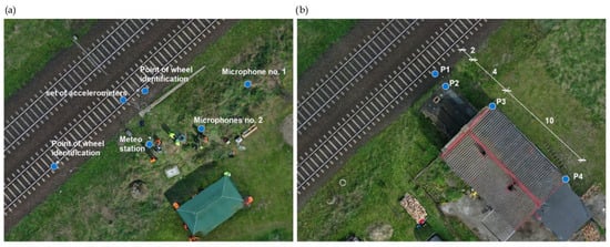
Figure 11.
Distribution of monitoring devices on the situational plan: (a) sensors (placed along the rail track) of the START, VEHICLE, RAIL VIBRATIONS modules, measurement points for noise monitoring in the NOISE module used with the meteorological station of the METEO module; (b) locations of vibration sensors in the ground and on a construction structure (GROUND VIBRATIONS module)—campaign 1.
Figure 12 shows a situational plan from Campaign 2 (UAV imagery) with the overlaid layout of measurement modules (controllers and sensors), while Figure 13 provides a detailed diagram of the spatial configuration of the SSN as implemented in Campaign 2.
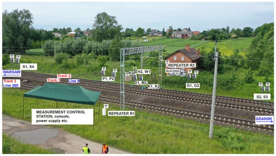
Figure 12.
Situational plan (UAV imagery) with the overlaid topology of the SSN—campaign 2.
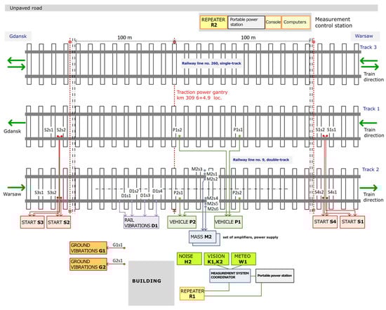
Figure 13.
Configuration of the SSN adapted to the location of Campaign 2 (detailed schematic).
For noise measurement, a class 1 noise monitoring station (Svantek SV 307A) [72] was used in conjunction with a compact meteorological station (Gill MaxiMet GMX600) [73]. These devices form the NOISE and METEO modules. The noise monitoring station records the acoustic signal continuously, saving files in WAV format on an SD memory card. To verify the reliability of the acoustic signal, the START and VEHICLE modules are used. The VISION module, equipped with Basler acA2040-90um cameras [74], appropriate lenses, and IR (Infrared) filters, is employed to identify the vehicle in the recorded acoustic signal. The RAIL VIBRATIONS and GROUND VIBRATIONS modules are used for measuring vibrations in the rail tracks and surrounding objects, respectively.
3. Results
3.1. Analysis of Acoustic Signals for Identification of Acoustic Events
In the analysis of acoustic signals, segmenting the signal based on individual acoustic events is essential. For this purpose, the algorithm uses data recorded by the VEHICLE module in the form of boundary times (start and end of the measurement), which are then stored in the MSC for each passing vehicle. The exemplary data is shown in Table 1. In the first column, the serial number is stored, while the second and third columns contain the start and end times of the measurement, respectively. The fourth column stores a logical parameter with a value of 1 or 0, indicating the validity of the measurement according to the standard [36], in relation to noise evaluation rules (for example, based on meteorological conditions).

Table 1.
Time Periods data for subsequent events.
Based on the time periods data (TP), the signal is filtered, and time windows containing train passages are saved to tables. Figure 14 presents the time windows of acoustic events, numbered from 1 to 11, illustrated using recorded sound level measurements with FAST time weighting and A-weighting correction, denoted as . The definition of the metric is given by Equation (7). This indicator is recommended by the standard [36] and is widely used in noise analysis.
where
—the equivalent sound level within a time window (0.125 s in the present study), interpreted as the signal power expressed in [dB];
—the sound energy within a given interval [J];
—the reference energy [J].

Figure 14.
Visualization of sample acoustic event segments according to the standard [36]—results from campaign 1.
If the value in column 4 of the TP table is 0, it indicates that the signal cannot be considered for further analysis due to factors such as rainfall or the passage of another train on an adjacent track. Such a measurement is classified as invalid and non-compliant with the applicable regulations [36]. An example of this is shown for events number 8 and 9, which are highlighted in red in Figure 13.
When sampling for analysis, it is crucial to meet the conditions outlined in [25], which pertain to the difference between the background noise level and the noise level of the train passage, as well as the detection of the vehicle’s front and rear in the analyzed signal. The continuous noise measurement concept allows for comparing the background noise level to the passage level, while vehicle detection in the acoustic signal is achieved through the sensor locations of the VEHICLE module along the measurement track. Figure 14 presents also the for the recorded events. The equivalent noise level can be understood as the energy-averaged sound level during the interval in which the train approaches and recedes from the measurement point, within a dynamic range of 10 dB. The sample range used for the determination of together with its level, is indicated by a horizontal line in blue, or red—marking acoustic events classified as non-significant, i.e., not fulfilling the thresholds adopted for environmental assessment. The equivalent event value was derived in accordance with [36]:
where
—The equivalent level within the acoustic event, expressed in [dB];
—the sound level in [dB] at the i-th sample;
—the number of samples of the averaged range of signal.
3.2. Analysis of Ground Vibrations to Determine the Impact of Vibration Levels on Building Structures
The selected algorithms were tested on real measurement data collected during field tests. The tests were conducted on a building located in the direct vicinity of an operational railway line (Figure 11). Horizontal acceleration signals () from three measurement points (marked as P2, P3, P4 in Figure 11b) were used. The sensors were installed at the corners of structural walls near the ground level. The combined acceleration signals generated by the passage of selected rolling stock are shown in Figure 15. The signals were generated by the vehicles in the following order: three freight trains (cargo), a single locomotive (loco), an InterCity passenger train (passenger), a draisine, an electric traction unit, and a freight train (cargo), as indicated in the description of Figure 15.
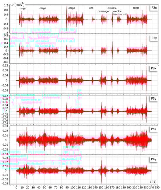
Figure 15.
Recorded measurement signals at points P2, P3, and P4 in the horizontal directions (x and y)—results from campaign 1.
The presented set of acceleration signals demonstrates a wide variation in amplitude levels originating from different types of rail vehicles. The position of the measurement point (distance from the source) also significantly affects the relative amplitude levels of selected vehicles; for example, at point P4 (see Figure 10), the most significant effects came from the passenger train, whereas at point P1, much higher amplitudes were generated by freight trains. The presented signals illustrate the complexity of wave propagation phenomena, highlighting the absolute need to integrate these data with other parameters, such as train speed or the frequencies of the generated vibrations.
Figure 16 shows the results of the one-third octave analysis (Block 1/3 OBB) of the acceleration signals from Figure 15. The building was classified into the DIS-I scale. The results indicate a noticeable impact of vibrations on the building. At the measurement point P2, vibration amplitudes occurred in the second damage zone, reaching the boundary between zones II and III at maximum. Such vibration levels do not pose a threat to the building’s structure; however, they may cause accelerated wear and initial cracks in elements like plaster.
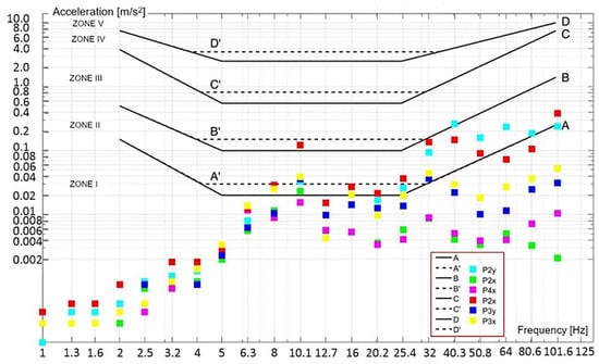
Figure 16.
Example of the operation of the one-third octave analysis algorithm for buildings (Block 1/3 OBB) applied to the measurement signals from Figure 13.
The remaining key characteristics of the measurement signals, including those from the modules responsible for rail vibration recording and the rail deflection indicator, will be presented for three representative train passages in Section 4.
4. Discussion
4.1. Identification of Vehicle Composition and Motion Parameters
The vehicle motion parameters include, among others, transit time, vehicle speed, number of axles, number of carriages, and total length. The measurement results from Campaign 1 and 2 enabled the implementation and validation of algorithms for determining these motion parameters.
The tests were carried out on heavily trafficked main railway lines. The mixed traffic structure, consisting of both freight and passenger trains, ensured train passages within a wide speed range from 30 to 200 km/h. The speed distribution of the recorded passages during Campaign 2 is presented in Figure 17, while the traffic intensity distribution is shown in Figure 18.
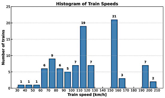
Figure 17.
Histogram of train and traction vehicle speeds recorded during Campaign 2.
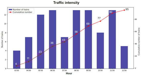
Figure 18.
Distribution of traffic intensity during Campaign 2.
Sample recordings of motion parameters are shown in Figure 19. The calculated speed allows for determining the distance between axles and the geometric dimensions of the train composition. The train speed along the measurement section may vary. From the recorded passage shown in Figure 19, it is clear that the instantaneous speed (rather than the average speed of the vehicle) must be taken into account when calculating the distance between the vehicle’s axles.
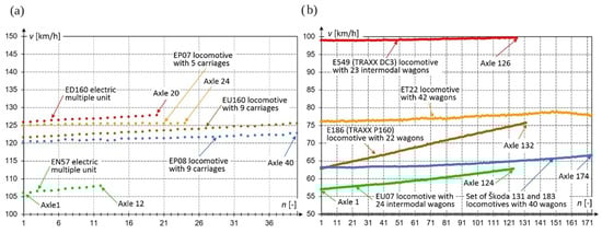
Figure 19.
Instantaneous speed of each vehicle axle determined based on the data processing algorithm from the VEHICLE module: (a) passenger trains; (b) freight trains.
The result of determining the distance between consecutive axles of the train is shown in Figure 20a. In this case, smaller distances correspond to the axle spacing within the bogies, while larger values represent the distances between the outer axles of adjacent carriages. The measurement module provides the length between the outermost axles of the vehicle, without accounting for the distance from the axle to the buffer edge. In the subsequent final processing, using the vehicle database, a more precise determination of the train length can be made.
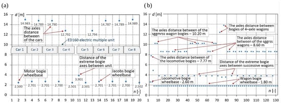
Figure 20.
Distances between consecutive axles n of a vehicle: (a) for the ED160 electric multiple unit; (b) for a freight train with the E186 locomotive and 22 flatbed wagons.
The identified structure of the rail vehicle is a two-car electric multiple unit, type Flirt, designated ED160, with a configuration of 20 axles: Bo’2′2’2’2’ + 2’2’2’2’Bo’ (see Figure 20a,b). The nominal axle spacing for the drive and running bogies is 2500 mm, while the spacing for the Jacob’s intercarriage bogies is 2700 mm. The approximate lengths of the carriages are as follows: outer motor cars (1 and 8)—15.0 m, middle carriages (2, 3, 6, and 7)—14.82 m, and carriages (4 and 5)—12.86 m. The nominal length of the traction unit is 152.9 m, while the measured length, including the dimension from the axle to the buffer edge, is 152.99 m. The individual axle-to-axle distances vary slightly from the nominal values by a few centimeters.
A more complex example of the registration of a passage of a long freight train with the E186 locomotive and 22 wagons is shown in Figure 20b. In this figure, the speed of all 132 axles of the vehicle is visible. The vehicle accelerates in this case, and its speed changes significantly along the measurement section.
The identified vehicle is a four-axle TRAXX P160 locomotive with the symbol E186, pulling 22 platform wagons in the following order: 1 × 6-axle type sggmrss, 5 × 6-axle sggrss, 3 × 6-axle sggmrss, 1 × 6-axle sggrss, 1 × 6-axle sggrmss, 1 × 4-axle sgnss, 1 × 4-axle, and 9 × 6-axle sggrss. The nominal axle spacing of the locomotive’s bogies is 2.6 m, and the spacing of the pivot pins is 10.44 m. The measured values are 2.6 m and 10.37 m, respectively. Regarding the wagons, all have a nominal axle spacing in the bogies of 1.800 m. For the 64 recorded bogies, the average measured axle spacing is 1.80 m with a standard deviation of 2 mm. Selected characteristic dimensions of the wagon consist and their types are shown in Figure 20b.
The comparison of the locomotive and wagon dimensions based on the technical documentation and measurement results shows that, by considering the instantaneous speed of each axle of the rail vehicle, the dimensions of the train composition can be determined with good accuracy.
Sample data, in the form of parameters characterizing train movements on the instrumented railway line (from an 8 h measurement session—campaign no. 2), are presented in Table 2 in a consolidated form. These parameters are calculated within the VEHICLE module and can be used for further analyses of noise and vibration. The developed system allows for the identification of trains across a relatively large number of categories (currently 36 types). For presentation purposes, however, six generic categories were defined. The first three correspond to electric multiple units (EMUs), classified according to their commercial operating speed. EMU200 refers to the ED250 Pendolino trains, which reach speeds of up to 200 km/h. The values presented in the table may be used for reporting or for more detailed assessments.
Table 2.
Train parameters, measurement campaign no. 2, double-track main line, measurement duration—8 h.
4.2. Selected Examples of Vibroacoustic Disturbance
Vibroacoustic disturbances generated during the passage of selected train compositions are presented through three representative cases. The cases are as follows:
- Case 1: ED250—electric multiple unit with a maximum operating speed of 200 km/h;
- Case 2: Passenger train hauled by locomotive EP07-1024, consisting of 5 carriages;
- Case 3: Freight train hauled by locomotive ET22-1130, consisting of 21 wagons.
These cases were chosen as they are sufficiently representative to illustrate the variability of results recorded by the SSN. The differences primarily arise from the speeds achieved by the trains, but they are also influenced by the technical condition and the general class of the vehicle. The ED250 train is a modern passenger composition with high technical performance and operates at high speeds, which results in increased vibroacoustic interactions. The freight train (Case 3) has a conventional design and does not reach high speeds; however, the technical condition of its components can affect the level of interactions. Train photos taken by camera of VISION module are shown in Figure 21.
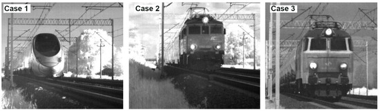
Figure 21.
Fronts of train cabins recorded by the VISION module.
In the charts comparing different signals, temporal synchronization was applied. In the implemented technical solutions of the sensor network, temporal discrepancies on the order of ~100 ms were obtained, which is a relatively good result and sufficient for identifying interactions at the level of individual bogies—or even individual axles. The synchronization accuracy was further improved in post-processing based on the known lengths of recorded records in the modules and the spatial distances between sensors, using the precise geodetic coordinates of the sensor placements.
4.2.1. Case 1—Electric Multiple Unit ED250
Based on the train composition parameters (data from the VEHICLE module), the train type was identified as a Pendolino ED250, running on track 2. The identified train composition parameters and instantaneous velocity are presented in Figure 22.
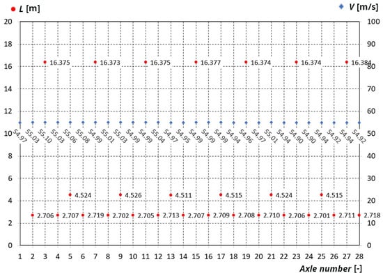
Figure 22.
Axle spacing and speed of the ED250 train—Case 1.
The train, traveling at approximately 200 km/h, generated vibrations and noise, with their characteristics shown in Figure 23. To enable visual synchronization in time and space, the independently recorded signals were presented with applied offsets. Except for the noise level, all values are shown numerically, without conversion to physical units. In the final phase of the software implementation, currently under development, these signals will be converted to physical quantities based on the known characteristics of the individual sensors.
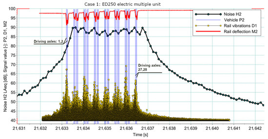
Figure 23.
Temporally synchronized signals from the modules: H2 (Noise), P2 (Vehicle), D1 (Rail vibrations), and M2 (Mass)—Case 1.
The signals shown in Figure 21 demonstrate proper correlation between the results concerning the observed phenomena. The charts reveal clear synchronization of peak values across all signals relative to the train’s layout, with the end bogies producing higher signal levels than those located in the middle of the train.
4.2.2. Case 2—Passenger Train Hauled by Locomotive EP07-1024, Consisting of 5 Carriages
Based on the train composition parameters the train type was identified as a passenger train hauled by locomotive EP07-1024 with 5 carriages, running on track 2. The identified train composition parameters and instantaneous velocity are presented in Figure 24.
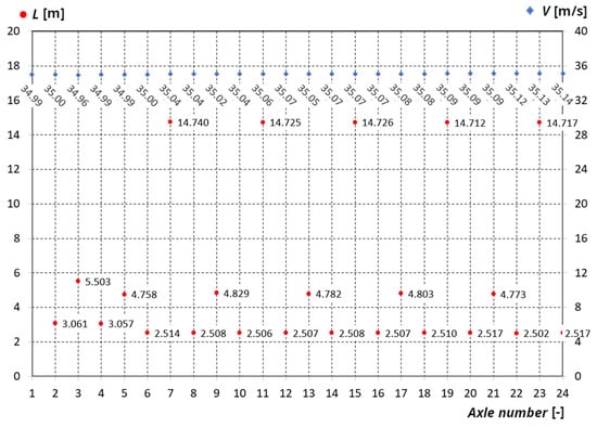
Figure 24.
Axle spacing and speed of the passenger train hauled by locomotive EP07-1024, consisting of 5 carriages—Case 2.
The train, traveling at approximately 125 km/h, produced vibrations and noise, with their characteristics shown in Figure 25. As in Case 1, offsets were applied to the independently recorded signals to enhance chart clarity.
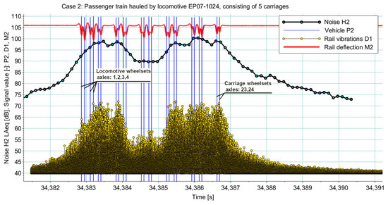
Figure 25.
Temporally synchronized signals from the modules: H2 (Noise), P2 (Vehicle), D1 (Rail vibrations), and M2 (Mass)—Case 2.
The signals in Figure 25, as in Case 1, show proper correlation between the results concerning the observed phenomena. Peak values across all signals are clearly synchronized with the train layout, with end bogies producing significantly higher levels than those in the middle. Exceedances of the measurement range of the applied sensor were observed in the acceleration signal. The correlation between vibrations and deflection reflects uneven axle loading, which in this case led to a correspondingly uneven noise distribution, approximately 10 dB higher than that of the relatively modern ED250 train.
4.2.3. Case 3—Freight Train Hauled by Locomotive ET22-1130, Consisting of 21 Wagons
Based on the train composition parameters the train type was identified as a freight train hauled by locomotive ET22-1130 with 21 wagons, running on track 2. The identified train composition parameters and instantaneous velocity are presented in Figure 26.
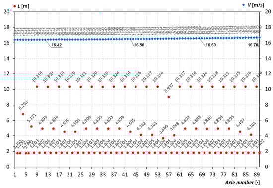
Figure 26.
Axle spacing and speed of the freight train hauled by locomotive ET22-1130, consisting of 21 wagons.
The freight train, traveling at approximately 60 km/h, produced vibrations and noise, with their characteristics shown in Figure 27.
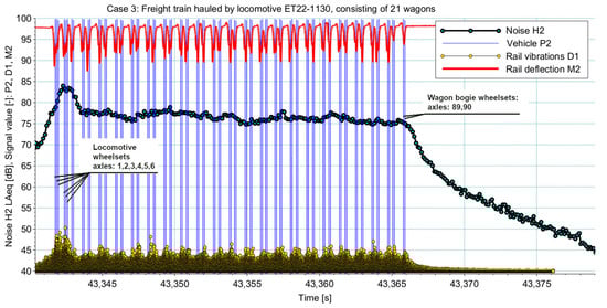
Figure 27.
Temporally synchronized signals from the modules: H2 (Noise), P2 (Vehicle), D1 (Rail vibrations), and M2 (Mass)—Case 3.
The signals in Figure 26, as in Cases 1 and 2, show a proper correlation of the results concerning the observed phenomena. Extreme values are clearly synchronized with the train layout. The ET22 locomotive bogies produced substantially higher vibration and noise levels than the tank wagon bogies. Of the three passages, this case exhibits the lowest overall noise and vibration levels, particularly during the wagon passages, which is clearly related to the train’s lower speed.
Figure 28 presents composite plots illustrating the characteristics of noise (Figure 28a) and rail vibrations (Figure 28b) during the passages of individual trains (Cases 1–3). The identified acoustic events are displayed along the time axis in a manner that enables their visual comparison. For each event, the equivalent noise level was calculated according to Equation (7). In the case of passage Case 2, acceleration values exceeding 50 g were observed. Considering that the applied sensor is characterized by linearity up to 50 g, these values fall beyond the reliable measurement range. Such values are indicated in Figure 28b accordingly (unreliable samples). In addition, samples exceeding 100 g (sensor’s exceedance limit) were also recorded. These samples are captured by a separate controller channel as OR samples (over range). Based on this event, it is recommended to use accelerometers with a doubled acceleration amplitude range.
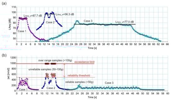
Figure 28.
Comparison of selected events (Cases 1–3): (a) noise; (b) rail vibration: envelope of rail acceleration.
In addition, for each event the Sound Exposure Level () [53] was calculated in accordance with Equation (8). is interpreted as the equivalent noise level lasting exactly one second and serves as a useful metric for comparing noise from sources that generate disturbances of varying durations. By definition, the Sound Exposure Level (SEL) is a measure of the sound energy of an event; therefore, in the logarithmic scale, a term of is added to the mean sound power of the event . This relationship can be expressed as follows:
where
—Sound Exposure Level normalized to a one-second time interval, expressed in [dB];
—denotes the event duration in seconds, normalized to one second, used in the calculation of .
Table 3 presents the basic noise and vibration parameters for the events Case 1–Case 3. The first column lists the train passage speed, while the second column shows the maximum values of the noise levels for each event. The third column contains the calculated equivalent noise level for the given event, according to Equation (7). The fourth column presents the values calculated using Equation (8). The last, fifth column provides the maximum values of the rail vibration envelope measured by one of the sensors.
Table 3.
Noise and vibration indicators in Cases 1–3.
Analysis of the data presented in Figure 28 and Table 2 indicates that the operational characteristics of the trains had a significant influence on the observed noise and vibration levels. Event 1 involved the ED250, a modern train design. Although its high speed generated relatively elevated noise and vibration levels, these levels were fairly uniform, and the short passage duration resulted in a low overall energetic impact. In contrast, event 2 featured a train of a typical late-20th-century design, which produced higher impact levels compared to event 1, despite a substantially lower passage speed. The lowest noise and vibration levels were recorded during the freight train passage (ET22), even though the locomotive design is outdated; however, the longer passage duration led to a relatively high energetic impact. Overall, the passage in event 2 represented the least favorable case in terms of environmental impact.
5. Conclusions
The conducted research demonstrated that the developed measurement system is capable of effectively recording and analyzing vibroacoustic phenomena in railway transport. Field measurement sessions on railway lines revealed clear correlations between train parameters—such as vehicle type, axle configuration, and travel speed—and the levels of noise and vibration propagating in the surrounding environment. These phenomena are interdependent, and their analysis requires synchronized monitoring of multiple parameters within a well-defined sensor network.
The measurement system presented in this work enables fully automated data acquisition on operational railway lines. Its prototype was tested during three multi-hour measurement campaigns. The results and their verification indicate a high level of effectiveness in identifying train types, speeds, axle configurations, impacts on track structures, as well as the resulting vibrations and noise.
Signal synchronization within the sensor network, with deviations on the order of 100 ms, allows processing and interpretation at the resolution of individual bogies and even single axles. This level of synchronization facilitates further analyses to identify correlations between train parameters and vibroacoustic effects, supporting effective management of the environmental impact of railway traffic.
Author Contributions
Conceptualization: P.C., K.K., A.W. and R.L.; Data curation: K.K., P.C., M.M., S.J., M.S. and N.K.-B.; Formal analysis: P.C., K.K. and M.M.; Funding acquisition: P.C., K.K., A.W., R.L. and S.G.; Investigation: P.C., K.K., R.L., M.S., M.M., A.W., L.J., J.S., S.J., S.G., T.W., K.D., N.K.-B., P.B. and K.S.; Methodology: P.C., K.K., R.L., M.S., M.M., A.W., L.J., P.B., K.S., J.S., S.G., T.W. and K.D.; Software: M.M., P.C., K.K. and L.J.; Supervision: P.C., K.K. and A.W.; Project administration: P.C.; Resources: P.C., A.W., K.K. and M.M.; Validation: P.C., K.K., R.L. and M.M.; Visualization: P.C., K.K., M.M. and M.S.; Writing—original draft: P.C., K.K., M.M., R.L. and M.S.; Writing—review and editing: P.C., K.K. and M.M. All authors have read and agreed to the published version of the manuscript.
Funding
The National Centre for Research and Development (NCBR) and PKP Polskie Linie Kolejowe S.A. (Polish State Railways Infrastructure Manager). The project entitled “A system for precise monitoring of the impact of railway traffic on the environment, taking into account information on operational, technical and environmental data” is being carried out within the frame-work of the NCBR–PKP PLK S.A. Joint Initiative “Research and Development in Railway Infrastructure–BRIK2” during the period from November 1, 2022, to October 31, 2025. Project acronym: InfraNoise. Project Funding Agreement: BRIK2/0020/2022.
Institutional Review Board Statement
Not applicable.
Informed Consent Statement
Not applicable.
Data Availability Statement
The measurement data presented in this work cannot be made publicly available in full due to ethical considerations related to the research conducted on behalf of the railway infrastructure manager.
Acknowledgments
The authors wish to sincerely thank the PKP PLK Railway Line Division in Gdynia for their valuable support in conducting research on operational railway lines.
Conflicts of Interest
The authors declare no conflicts of interest. The funders had no role in the design of the study; in the collection, analyses, or interpretation of data; in the writing of the manuscript; or in the decision to publish the results.
Abbreviations
The following abbreviations are used in this manuscript:
| IIoT | Industrial Internet of Things |
| CNOSSOS-EU | Common Noise Assessment Methods in Europe |
| RFID | Radio Frequency Identification |
| GSM | Global System for Mobile Communications |
| SSN | Spatial Sensor Network |
| MSC | Measurement System Coordinator |
| 1/3 OBB | One-third Octave Band for buildings |
| SC | Signal Centering |
| SF | Signal Filtering |
| SA | Spectral Analysis |
| DIS | Dynamic Influence Scales |
| DFT | Discrete Fourier Transform |
| RMS | Root Mean Square |
| PSD | Power Spectral Density |
| ANPSD | Averaged Normalized Power Spectral Density |
| TP | Time Periods data |
| SEL | Sound Exposure Level |
References
- Connolly, D.P.; Marecki, G.P.; Kouroussis, G.; Thalassinakis, I.; Woodward, P.K. The growth of railway ground vibration problems—A review. Sci. Total Environ. 2016, 568, 1276–1282. [Google Scholar] [CrossRef]
- U.S. Department of Transportation. National Transportation Noise Map. Bureau of Transportation Statistics. Available online: https://maps.dot.gov/BTS/NationalTransportationNoiseMap/ (accessed on 16 October 2025).
- International Union of Railways (UIC). Railway Induced Vibration—State of the Art Report. International Union of Railways (UIC); International Union of Railways (UIC): Paris, France, 2017. [Google Scholar]
- Thompson, D. Railway Noise and Vibration. Mechanisms, Modelling and Means of Control; Elsevier: Amsterdam, The Netherlands, 2024; ISBN 9780128219799. [Google Scholar]
- Fiorini, C.V. Railway noise in urban areas: Assessment and prediction on infrastructure improvement combined with settlement development and regeneration in central Italy. Appl. Acoust. 2022, 185, 108413. [Google Scholar] [CrossRef]
- Luo, Y.-K.; Song, L.-Z.; Zhang, C.; Ni, Y.-Q. Experimental evaluation and numerical interpretation of various noise mitigation strategies for in-service elevated suburban rail. Measurement 2023, 219, 113276. [Google Scholar] [CrossRef]
- Tutmez, B.; Baranovskii, A. Quantifying uncertainty in railway noise measurement. Measurement 2019, 137, 1–6. [Google Scholar] [CrossRef]
- Licitra, G.; Fredianelli, L.; Petri, D.; Vigotti, M.A. Annoyance evaluation due to overall railway noise and vibration in Pisa urban areas. Sci. Total Environ. 2016, 568, 1315–1325. [Google Scholar] [CrossRef] [PubMed]
- Huang, L.; Sun, Z.; Yu, C.; Zhang, Y.; Yan, B. The noise exposure of urban rail transit drivers: Hazard classification, assessment, and mitigation strategies. Appl. Sci. 2024, 14, 7388. [Google Scholar] [CrossRef]
- He, Y.; Zhang, Y.; Yao, Y.; He, Y.; Sheng, X. Review on the prediction and control of structural vibration and noise in buildings caused by rail transit. Buildings 2023, 13, 2310. [Google Scholar] [CrossRef]
- Ouakka, S.; Verlinden, O.; Kouroussis, G. Railway ground vibration and mitigation measures: Benchmarking of best practices. Railw. Eng. Sci. 2022, 30, 2310. [Google Scholar] [CrossRef]
- Pieren, R.; Heutschi, K.; Wunderli, J.M.; Snellen, M.; Simons, D.G. Auralization of railway noise: Emission synthesis of rolling and impact noise. Appl. Acoust. 2017, 127, 34–45. [Google Scholar] [CrossRef]
- Yan, H.; Xie, S.; Jing, K.; Feng, Z. A Review of Recent Research into the Causes and Control of Noise during High-Speed Train Movement. Appl. Sci. 2022, 12, 7508. [Google Scholar] [CrossRef]
- Schweizerische Eidgenossenschaft. Richtlinie Lärmschutz bei Eisenbahnanlagen. Bundesamt für Verkehr (BAV), 15 September 2023. Available online: https://www.bav.admin.ch/ (accessed on 24 April 2025).
- Laerm Monitoring. Messverfahren. (n.d.). Available online: https://www.laerm-monitoring.de/Messverfahren (accessed on 24 April 2025).
- Liu, X.; Xiao, Y.; Jiang, H.; Guo, Y.; Yu, M.; Tan, W. Analogical Assessment of Train-Induced Vibration and Radiated Noise in a Proposed Theater. Sensors 2023, 23, 505. [Google Scholar] [CrossRef]
- Tao, Z.; Hu, Z.; Wu, G.; Huang, C.; Zou, C.; Ying, Z. Train-Induced Vibration Predictions Based on Data-Driven Cascaded State-Space Model. Buildings 2022, 12, 114. [Google Scholar] [CrossRef]
- Niu, D.; Deng, Y.; Mu, H.; Chang, J.; Xuan, Y.; Cao, G. Attenuation and propagation characteristics of railway load-induced vibration in a loess area. Transp. Geotech. 2022, 37, 100858. [Google Scholar] [CrossRef]
- Zheng, H.; Yan, W. Field and numerical investigations on the environmental vibration and the influence of hill on vibration propagation induced by high-speed trains. Constr. Build. Mater. 2022, 357, 129378. [Google Scholar] [CrossRef]
- Mikielewicz, M.; Jakubczyk-Gałczyńska, A.; Jankowski, R. Investigating the Effects of Ground-Transmitted Vibrations from Vehicles on Buildings and Their Occupants, with an Idea for Applying Machine Learning. Appl. Sci. 2025, 15, 1689. [Google Scholar] [CrossRef]
- Aela, P.; Chi, H.-L.; Fares, A.; Zayed, T.; Kim, M. UAV-based studies in railway infrastructure monitoring. Autom. Constr. 2024, 167, 105714. [Google Scholar] [CrossRef]
- Du, C.; Dutta, S.; Kurup, P.; Yu, T.; Wang, X. A review of railway infrastructure monitoring using fiber optic sensors. Sens. Actuators A Phys. 2020, 303, 111728. [Google Scholar] [CrossRef]
- Kowalska-Koczwara, A. Impact of selected sources of transport vibrations on the perception of vibrations by people in buildings. Vibroengineering Procedia 2019, 27, 88–92. [Google Scholar] [CrossRef]
- Zhang, C.; Kordestani, H.; Shadabfar, M. A combined review of vibration control strategies for high-speed trains and railway infrastructures: Challenges and solutions. J. Low Freq. Noise Vib. Act. Control 2023, 42, 272–291. [Google Scholar] [CrossRef]
- Licow, R.; Tomaszewski, F. Application of vibration signals in railway track diagnostics using a mobile railway platform. Arch. Transp. 2024, 71, 127–145. [Google Scholar] [CrossRef]
- Wilk, A.; Koc, W.; Specht, C.; Skibicki, J.; Judek, S.; Karwowski, K.; Chrostowski, P.; Szmagliński, J.; Dąbrowski, P.; Czaplewski, K.; et al. Innovative mobile method to determine railway track axis position in global coordinate system using position measurements performed with GNSS and fixed base of the measuring vehicle. Measurement 2021, 175, 109016. [Google Scholar] [CrossRef]
- Javaid, O.; Choi, D.-H. Effect of track irregularities on the response of two-way railway tracks. Appl. Sci. 2019, 10, 11. [Google Scholar] [CrossRef]
- Jiang, X.; Wang, S. Railway panorama: A fast inspection method for high-speed railway infrastructure monitoring. IEEE Access 2021, 9, 150889–150902. [Google Scholar] [CrossRef]
- Teng, J.; Long, X.; Yang, Q.; Jing, G.; Liu, H. Semi-Conv-DETR: A railway ballast bed defect detection model integrating convolutional augmentation and semi-supervised DETR. Transp. Geotech. 2024, 48, 101334. [Google Scholar] [CrossRef]
- Licow, R.; Szabłowska, D. Assessment of acoustic climate in passenger space of EN57 series electric multiple unit. Rail Veh. 2020, 2020, 45–53. [Google Scholar] [CrossRef]
- Li, L.; Thompson, D.; Xie, Y.; Zhu, Q.; Luo, Y.; Lei, Z. Influence of rail fastener stiffness on railway vehicle interior noise. Appl. Acoust. 2019, 145, 69–81. [Google Scholar] [CrossRef]
- Sun, L.; Shang, Z.; Xia, Y.; Bhowmick, S.; Nagarajaiah, S. Review of Bridge Structural Health Monitoring Aided by Big Data and Artificial Intelligence: From Condition Assessment to Damage Detection. J. Struct. Eng. 2020, 146, 04020073. [Google Scholar] [CrossRef]
- Traquinho, N.; Vale, C.; Ribeiro, D.; Meixedo, A.; Montenegro, P.; Mosleh, A.; Calçada, R. Damage Identification for Railway Tracks Using Onboard Monitoring Systems in In-Service Vehicles and Data Science. Machines 2023, 11, 981. [Google Scholar] [CrossRef]
- Hoelzl, C.; Arcieri, G.; Ancu, L.; Banaszak, S.; Kollros, A.; Dertimanis, V.; Chatzi, E. Fusing Expert Knowledge with Monitoring Data for Condition Assessment of Railway Welds. Sensors 2023, 23, 2672. [Google Scholar] [CrossRef] [PubMed]
- Faccini, L.; Karaki, J.; Di Gialleonardo, E.; Somaschini, C.; Bocciolone, M.; Collina, A. A Methodology for Continuous Monitoring of Rail Corrugation on Subway Lines Based on Axlebo Acceleration Measurements. Appl. Sci. 2023, 13, 3773. [Google Scholar] [CrossRef]
- EN ISO 3095:2013; Acoustics—Railway Applications—Measurement of Noise Emitted by Railbound Vehicles (ISO 3095:2013). International Organization for Standardization: Geneva, Switzerland, 2013.
- Meng, Q.; Zhu, S. Developing iot sensing system for construction-induced vibration monitoring and impact assessment. Sensors 2020, 20, 6120. [Google Scholar] [CrossRef]
- Castillo-Mingorance, J.M.; Sol-Sánchez, M.; Moreno-Navarro, F.; Rubio-Gámez, M.C. A critical review of sensors for the continuous monitoring of smart and sustainable railway infrastructures. Sustainability 2020, 12, 9428. [Google Scholar] [CrossRef]
- Shao, Z.; Bai, W.; Dai, J.; Yu, H.; Tong, Y. Monitoring and analysis of railway-induced vibration and structure-borne noise in a transit oriented development project. Structures 2023, 57, 105097. [Google Scholar] [CrossRef]
- Khan, D.; Burdzik, R. Measurement and analysis of transport noise and vibration: A review of techniques, case studies, and future directions. Measurement 2023, 220, 113354. [Google Scholar] [CrossRef]
- Marques, G.; Pitarma, R. A real-time noise monitoring system based on internet of things for enhanced acoustic comfort and occupational health. IEEE Access 2020, 8, 139741–139755. [Google Scholar] [CrossRef]
- Verheijen, E.; Roovers, M.S.; van den Brink, J.W. Railway noise statistics by monitoring stations-input for Dutch prediction method RMR and track access charging. In Noise and Vibration Mitigation for Rail Transportation Systems, Proceedings of the 9th International Workshop on Railway Noise, Munich, Germany, 4–8 September 2007; Springer: Berlin/Heidelberg, Germany, 2007; pp. 165–171. [Google Scholar] [CrossRef]
- Liu, Q.; Xu, L.; Feng, Q. Intelligent monitoring of vibration and structural-borne noise induced by rail transit. Intell. Transp. Infrastruct. 2023, 2, liad013. [Google Scholar] [CrossRef]
- Li, Y.; Liu, L.; Li, Z. Noise mapping technology of high-speed railway based on GIS. J. Geogr. Cartogr. 2022, 5, 16–24. [Google Scholar] [CrossRef]
- Khan, D.; Burdzik, R. A review on different regulation for the measurement of transport noise and vibration. J. Meas. Eng. 2023, 11, 196–213. [Google Scholar] [CrossRef]
- EN 15610:2019; Railway Applications—Acoustics—Rail and Wheel Roughness Measurement Related To Noise Generation. European Committee for Standardization: Brussels, Belgium, 2019.
- Track Noise Measurement Guidelines—A Methodology to Measure and Compare Noise Emissions During Train Pass-Bys; Ed. no.1.; UIC Railway Technical Publications: Paris, France, 2023; Available online: https://shop.uic.org/en/1-laying-and-maintenance-of-track/14479-track-noise-measurement-guidelines-a-methodology-to-measure-and-compare-noise-emissions-during-train-pass-bys.html (accessed on 10 September 2025).
- EN 15461:2008+A1-2010; Railway Applications—Noise Emission—Characterisation of the Dynamic Properties of Track Sections for Pass by Noise Measurements. iTeh, Inc.: Newark, DE, USA, 2010.
- Commission Regulation (EU) No 1304/2014 of 26 November 2014 on the Technical Specification for Interoperability Relating to the Subsystem ‘Rolling Stock—Noise’ Amending Decision 2008/232/EC and Repealing Decision 2011/229/EU. Available online: https://eur-lex.europa.eu/eli/reg/2014/1304/2023-09-28/eng (accessed on 16 October 2025).
- Rosin, C.; Sineau, M.; Regairaz, J.-P.; Cordoliani, T. Railway noise monitoring—A tool to analyse in detail the evolution of noise over time. In Proceedings of the 10th Convention of the European Acoustics Association, Turin, Italy, 11–15 September 2023; pp. 6435–6442. [Google Scholar] [CrossRef]
- European Commission. CNOSSOS-EU (Common Noise Assessment Methods in Europe). European Commission. Available online: https://ec.europa.eu (accessed on 16 October 2025).
- PN-EN IEC 60942:2018; Electroacoustics—Acoustic Calibrators. Polish Committee for Standardization: Warsaw, Poland, 2018.
- PN-EN IEC 61672-1:2024; Electroacoustics—Sound Level Meters—Part 1: Specifications. Polish Committee for Standardization: Warsaw, Poland, 2024.
- PN-EN IEC 61672-3:2013; Electroacoustics—Sound Level Meters—Part 3: Periodic Calibration Procedures. Polish Committee for Standardization: Warsaw, Poland, 2013.
- PN-EN ISO 17025:2018; General Requirements for the Competence of Testing and Calibration Laboratories. Polish Committee for Standardization: Warsaw, Poland, 2018.
- Available online: www.bav.admin.ch/bav/de/home/verkehrsmittel/eisenbahn/bahninfrastruktur/ausbauprogramme/weitere-ausbauprogramme/laermsanierung/monitoring.html (accessed on 24 April 2025).
- Dinhobl, G. Railway noise term monitoring: Experiences and standarisation. In Proceedings of the 10th Convention of the European Acoustics Association, Turin, Italy, 11–15 September 2023; pp. 225–232. [Google Scholar] [CrossRef]
- de Weert, Y.; Gkiotsalitis, K.; van Berkum, E. Improving the scheduling of railway maintenance projects by minimizing passenger delays subject to event requests of railway operators. Comput. Oper. Res. 2024, 165, 106580. [Google Scholar] [CrossRef]
- McCollough, J.D.; Sargsyan, G.; Luo, Z. The impact of declining birth rates on future infrastructure maintenance costs per capita. J. Econ. Stud. 2022, 50, 1121–1129. [Google Scholar] [CrossRef]
- Available online: https://www.adts.it/track-geometry-measurement-system/ (accessed on 10 October 2025).
- Available online: https://www.voestalpine.com/railway-systems/en/products/zentrak-train-detection-monitoring/ (accessed on 10 October 2025).
- Available online: https://www.mobility.siemens.com/global/en/portfolio/digital-solutions-software/digital-services/measurement-monitoring.html (accessed on 10 October 2025).
- Available online: https://www.mermecgroup.com/15/measurement-br-trains-e-systems.php (accessed on 10 October 2025).
- Wróbel, J.; Bury, P.; Zając, M.; Kierzkowski, A.; Tubek, S.; Blaut, J. Fault Detection and Diagnostic Methods for Railway Systems—A Literature Survey. Adv. Sci. Technol. Res. J. 2024, 18, 361–391. [Google Scholar] [CrossRef]
- Ghiasi, R.; Lestoille, N.; Diaine, C.; Malekjafarian, A. Unsupervised domain adaptation for drive-by condition monitoring of multiple railway tracks. Eng. Appl. Artif. Intell. 2025, 139, 109516. [Google Scholar] [CrossRef]
- Aela, P.; Cai, J.; Jing, G.; Chi, H.-L. Vision-based monitoring of railway superstructure: A review. Constr. Build. Mater. 2024, 442, 137385. [Google Scholar] [CrossRef]
- Luo, L.; Qin, H.; Song, X.; Wang, M.; Qiu, H.; Zhou, Z. Wireless Sensor Networks for Noise Measurement and Acoustic Event Recognitions in Urban Environments. Sensors 2020, 20, 2093. [Google Scholar] [CrossRef]
- Alsina-Pagès, R.M.; Bellucci, P.; Zambon, G. Smart Wireless Acoustic Sensor Network Design for Noise Monitoring in Smart Cities. Sensors 2020, 20, 4765. [Google Scholar] [CrossRef]
- Armijo, A.; Zamora-Sanchez, D. Integration of Railway Bridge Structural Health Monitoring into the Internet of Things with a Digital Twin: A Case Study. Sensors 2024, 24, 2115. [Google Scholar] [CrossRef]
- Sujon, M.; Dai, F. Application of weigh-in-motion technologies for pavement and bridge response monitoring: State-of-the-art review. Autom. Constr. 2021, 130, 103844. [Google Scholar] [CrossRef]
- Pintao, B.; Mosleh, A.; Vale, C.; Montenegro, P.; Costa, P. Development and Validation of a Weigh-in-Motion Methodology for Railway Tracks. Sensors 2022, 22, 1976. [Google Scholar] [CrossRef] [PubMed]
- Available online: https://svantek.com/products/sv-307a-noise-monitoring-station/ (accessed on 10 October 2025).
- Available online: https://gillinstruments.com/wp-content/uploads/2024/02/1957-010-MaxiMet-GMX600-Issue-12.pdf (accessed on 10 October 2025).
- Available online: https://www.baslerweb.com/en/shop/aca2040-90umnir (accessed on 10 October 2025).
- PN-B-02171:2017-06; Assessment of the Impact of Vibrations on People in Buildings. PKN: Warsaw, Poland, 2017. (In Polish)
- Zhang, Z.; Ma, F.; Zhang, B. Vibration measurement of long-span floors in high-speed railway station. J. Vibroengineering 2018, 20, 2705–2719. [Google Scholar] [CrossRef]
- Available online: https://www.analog.com (accessed on 10 October 2025).
- Available online: https://www.strainsense.co.uk/ (accessed on 10 October 2025).
- Available online: https://www.ifm.com/pl/en/product/IIS284 (accessed on 10 October 2025).
Disclaimer/Publisher’s Note: The statements, opinions and data contained in all publications are solely those of the individual author(s) and contributor(s) and not of MDPI and/or the editor(s). MDPI and/or the editor(s) disclaim responsibility for any injury to people or property resulting from any ideas, methods, instructions or products referred to in the content. |
© 2025 by the authors. Licensee MDPI, Basel, Switzerland. This article is an open access article distributed under the terms and conditions of the Creative Commons Attribution (CC BY) license (https://creativecommons.org/licenses/by/4.0/).