MAC-I2P: I2P Registration with Modality Approximation and Cone–Block–Point Matching

Abstract

The misaligned geometric representation between images and point clouds and the different data densities limit the performance of I2P registration. The former hinders the learning of cross-modal features, and the latter leads to low-quality 2D–3D matching. To address these challenges, we propose a novel I2P registration framework called MAC-I2P, which is composed of a modality approximation module and a cone–block–point matching strategy. By generating pseudo-RGBD images, the module mitigates geometrical misalignment and converts 2D images into 3D space. In addition, it voxelizes the point cloud so that the features of the image and the point cloud can be processed in a similar way, thereby enhancing the repeatability of cross-modal features. Taking into account the different data densities and perception ranges between images and point clouds, the cone–block–point matching relaxes the strict one-to-one matching criterion by gradually refining the matching candidates. As a result, it effectively improves the 2D–3D matching quality. Notably, MAC-I2P is supervised by multiple matching objectives and optimized in an end-to-end manner, which further strengthens the cross-modal representation capability of the model. Extensive experiments conducted on KITTI Odometry and Oxford Robotcar demonstrate the superior performance of our MAC-I2P. Our approach surpasses the current state-of-the-art (SOTA) by 8∼63.2% in relative translation error (RTE) and 19.3∼38.5% in relative rotation error (RRE). The ablation experiments also confirm the effectiveness of each proposed component.

1. Introduction

Determining the relative positions of multi-robots within a robot swarm serves as the prerequisite for accomplishing various intelligent applications, including SLAM (Simultaneous Localization and Mapping), robot navigation, and scene understanding [1]. To achieve this goal, robots are equipped with multiple sensors, from whose data pose estimation is performed [2,3]. The pivotal factor in pose estimation lies in the precise alignment of multiple sensor data originating from either intra-modality or inter-modality sources, commonly referred to as registration [4]. Cameras and LiDARs, which are well-known for their exceptional environmental capturing capabilities, are extensively used in robot pose estimation [5,6]. Although numerous methodologies for intra-modality registration (e.g., image-to-image [7] and point cloud to point cloud registration [8]) have achieved noteworthy performance, the inter-modality registration between images and point clouds remains relatively limited exploration due to its inherent challenges.

Image-to-point cloud (I2P) registration refers to the estimation of the relative pose between a LiDAR and a camera via their measurements captured from the same scene [9]. Similar to intra-modality registration, achieving highly accurate correspondences is crucial for I2P registration performance. Early I2P registration approaches attempted to establish 2D–3D correspondences by keypoint detection and matching as shown in Figure 1a [10]. However, the discrepancies between images and point clouds pose challenges in designing cross-modality features, making it difficult to establish reliable 2D–3D correspondences. As a result, the performance of these methods remains unsatisfactory. Some recent studies [11,12] attempted to alleviate these discrepancies by constructing a shared feature space, and they are referred to as feature alignment-based methods. These approaches utilized neural networks to extract 2D and 3D features and aligned them using cross-attention. However, feature alignment-based methods only focus on addressing the misaligned feature space while overlooking the misalignment in geometry structures.

Owing to the effect of perspective projection, depth information is inevitably lost during image capture. In contrast, LiDAR accurately captures the geometric structure of the environment through distance measurement. This geometric misalignment poses challenges when attempting to construct cross-modality descriptions for images and point clouds. Therefore, in addition to feature space alignment, it is valuable to align images and point clouds in terms of geometric structures.

Besides, the different data densities and sensing ranges of images and point clouds render directly matching individual points with pixels a non-trivial task. Current methods typically establish 2D–3D correspondences by computing an all-pair distance matrix between points and pixels, which increases the number of outliers and introduces computational redundancy [9,11,12]. In fact, due to the difference in perception range, the co-view region between the camera and the LiDAR appears as a cone shape (see Figure 1c). This means that a considerable number of points and pixels are invalid matching candidates. Furthermore, caused by different data densities, even in the co-view region, a pixel may correspond to multiple points, and this matching ambiguity is difficult to avoid. Based on the above, establishing strict one-to-one correspondences in the same manner as in intra-modality registration is difficult in I2P registration.

To fill the aforementioned research gaps to a certain extent, in this work, we propose Image-to-Point cloud registration with Modality approximation And Cone–block–point matching, MAC-I2P for short. Specifically, we aim to recover the lost depth information from images to some extent and transform the 2D data to the 3D space (see Figure 1b). In this way, the misalignment in geometry structure between images and point clouds can be mitigated. Furthermore, a voxel-based network is leveraged for extracting point cloud features. This allows the application of 3D convolutions to capture the features of the voxelized point cloud. This approach bears similarity to the feature extraction employed in 2D backbones, thereby enhancing the repeatability of cross-modality features.

In addition, to overcome the matching ambiguity caused by different data densities and sensing ranges, a novel cone–block–point matching strategy is proposed to improve the quality of 2D–3D correspondences (see Figure 1c). This strategy no longer strives to establish strict one-to-one correspondences between points and pixels. Instead, it relaxes the matching criteria by progressively refining the matching candidates.

To summarize, our contributions are threefold:

(1)

A novel I2P registration framework based on the modality approximation and cone–block–point matching is proposed, named MAC-I2P. It learns cross-modality features by encouraging mutual approximation between images and point clouds and predicts 2D–3D correspondences based on hierarchical matching in an end-to-end manner.

(2)

A meticulous modality approximation module is designed. Specifically, we propose to recover the geometry structures of images and enable a similar feature extraction approach for both images and point clouds. This module not only alleviates the feature representation discrepancies between images and point clouds but also mitigates the currently overlooked misalignment in geometric structures.

(3)

A cone–block–point matching strategy for sparse LiDAR point clouds and dense images is introduced. It effectively addresses the matching ambiguity by gradually narrowing down the matching scope and significantly improves the quality of the 2D–3D matching.

(4)

Extensive experiments conducted on KITTI Odometry [13], Oxford Robotcar [14], and self-collected data demonstrate that MAC-I2P outperforms other SOTA methods in terms of registration performance.

The remainder of this paper is organized as follows: Section 2 introduces the related studies. Details of the proposed MAC-I2P are presented in Section 3. The experimental results are reported in Section 4. Finally, Section 5 concludes the paper.

2. Related Work

2.1. Intra-Modality Registration

2.1.1. Image Registration

Image registration aims to infer the relative pose between multiple images that capture the same scene from different locations [15]. Due to the lack of depth information, hand-crafted features based on color and texture are adopted to detect and describe the image’s keypoints [16]. Then these keypoints are matched through feature similarity measuring and the Perspective-n-Point (PnP) or Bundle Adjustment algorithm can be further applied to estimate the pose [17]. To save the step of designing hand-crafted features, some approaches extract keypoints by deep learning [18,19], which improves the robustness and accuracy of matching. Furthermore, some methods go a step further and aim to incorporate both feature learning and matching into neural networks, thus proposing a detection-then-matching learning framework. For example, SuperGlue [20] uses attention [21] to aggregate the global and local features, formulates the image matching problem as a graph matching problem, and determines the matching pairs by approximately linear distribution. Recently, keypoint-free methods have achieved impressive performance. These methods bypass the learning of keypoints and directly learn pixel-wise dense matching. The LoFTR series [22,23] are representative examples, which utilize a coarse-to-fine architecture. It first generates a large number of coarse-level matching candidates and then refines them at a fine level to obtain pixel-by-pixel matching. In addition, some researchers also explore the application of foundation models for image registration [7].

2.1.2. Point Cloud Registration

The development in point cloud registration (PCR) has also witnessed a similar progression as in image registration [8,24]. Early studies mainly establish correspondences based on keypoint matching [25,26]. Recently, learning-based approaches have achieved more accurate registration results. PointNetLK [27] no longer detects keypoints but directly learns point-wise features. It leverages feature metrics and the IC-LK algorithm to estimate the pose. PCRNet [28] replaces the IC-LK algorithm in PointNetLK with fully connected layers and directly infers the transformation matrix. In addition, there are several studies aimed at establishing more accurate correspondences. Some representative studies in this category are reviewed here. GeoTransformer [29] leverages self-attention and cross-attention for feature learning within individual point clouds and across multiple point clouds. It utilizes a local-to-global architecture to predict the transformation. Building upon GeoTransformer, ColorPCR [30] adopts a multi-stage geometry–color fusion approach to extract robust point features, thereby enabling accurate registration of colored point clouds. By constructing strict constraints to compute the inner-point confidence (ICC), Yuan et al. [31] achieved point cloud registration following the “pseudo-correspondence to inner-point estimation” procedure. MAC [32] adopts a non-deep learning approach to search for maximum clique subsets in matching pairs. Then, the SVD is utilized to estimate the rigid transformation corresponding to each maximum clique efficiently and select the optimal transformation guided by the reprojection error.

2.2. Inter-Modality Registration

Compared to intra-modality registration, the modality discrepancies between images and point clouds undoubtedly make inter-modality registration more challenging [33]. According to the way of correspondence building, previous studies can be categorized into two classes: keypoint-based methods and keypoint-free methods.

2D3D-MatchNet [10] is a representative keypoint-based method. This approach uses SIFT [16] and ISS [34] to extract 2D and 3D keypoints from images and point clouds, respectively, and employs neural networks to learn descriptors of these feature points, thereby facilitating the establishment of correspondences among keypoints. P2Net [35] adopts a dual fully convolutional framework to jointly detect and describe keypoints in images and RGBD point clouds, and determines the correspondences through peakness measurement. DGC-GNN [36] attempts to improve matching accuracy by using a global-to-local Graph Neural Network (GNN). It represents keypoints by gradually exploiting geometric and color cues. Similar to I2P registration, the purpose of LiDAR-camera calibration [37,38,39] is also to estimate the relative pose between the LiDAR and the camera. Current studies usually first extract line and plane features from images and point clouds, followed by establishing correspondences among these features and optimizing the relative pose by minimizing reprojection errors. However, LiDAR-camera calibration typically requires additional calibration targets or scenes with rich geometric information, and multiple frames of images and point clouds to ensure the calibration quality. This limits the flexibility of such algorithms.

Keypoint-free methods place greater emphasis on learning cross-modal features. DeepI2P [11] and CorrI2P [12] utilize attention to fuse the features of images and point clouds, allowing for the acquisition of cross-modal feature representations. DeepI2P adopts an inverse camera projection technique based on frustum classification results to estimate the pose. CorrI2P establishes 2D–3D correspondences at the pixel/point level using feature distance metrics. VP2P [9] introduces an end-to-end triplet network to learn a structured cross-modality latent space and optimizes the networks through a differentiable PnP solver. Based on the coarse-to-fine architecture, 2D3D-MATR [40] utilizes a multi-scale matching strategy to build 2D–3D correspondences. It achieves excellent performance in the task of matching images with dense RGBD point clouds. This limits the flexibility of such algorithms.

However, the methods mentioned above either focus on the fusion of cross-modal features [9,11,12] or rely on dense RGBD point clouds [40], overlooking the misaligned geometric information and different data densities between images and point clouds.

3. Methodology

3.1. Overview

Given a pair of partially overlapping observations, an RGB image $\mathbf{I}\in {\mathbb{R}}^{W\times H\times 3}$ and a LiDAR point cloud $\mathbf{P}\in {\mathbb{R}}^{N\times 3}$, where W and H are the width and height of the image respectively, and N is the number of points for the point cloud. The goal of I2P registration is to estimate the relative rigid transformation $\mathbf{T}\in \mathrm{SE}\left(3\right)$ between $\mathbf{I}$ and $\mathbf{P}$, where $\{\mathbf{T}=\left[\mathbf{R}\right|\mathbf{t}],\mathbf{R}\in \mathrm{SO}\left(3\right)|\mathbf{t}\in {\mathbb{R}}^3\}$. A natural and intuitive approach is to establish the 2D–3D correspondences, represented by $\mathcal{M}=\{({\mathbf{u}}_i,s|{\mathbf{u}}_i\in {\mathbb{R}}^2,{\mathbf{p}}_i\in {\mathbb{R}}^3\}$, and estimate the relative pose by minimizing the reprojection error as follows:

$${\mathbf{T}}^{*}=\underset{\mathbf{T}}{argmin}\sum _{{\mathbf{u}}_i,{\mathbf{p}}_i\in \mathcal{M}}{\parallel \pi (\mathbf{K},\mathbf{T},{\mathbf{p}}_i)-{\mathbf{u}}_i\parallel }^2,$$

(1)

where $\pi$ is the projection function from 3D space to image plane and $\mathbf{K}\in {\mathbb{R}}^{3\times 3}$ is the intrinsic matrix of the camera. Assuming accurate correspondences are established, Equation (1) can be iteratively solved by EPnP with RANSAC or Bundle Adjustment [17,41]. Therefore, the accuracy of 2D–3D correspondences becomes a crucial factor in determining the performance of I2P registration.

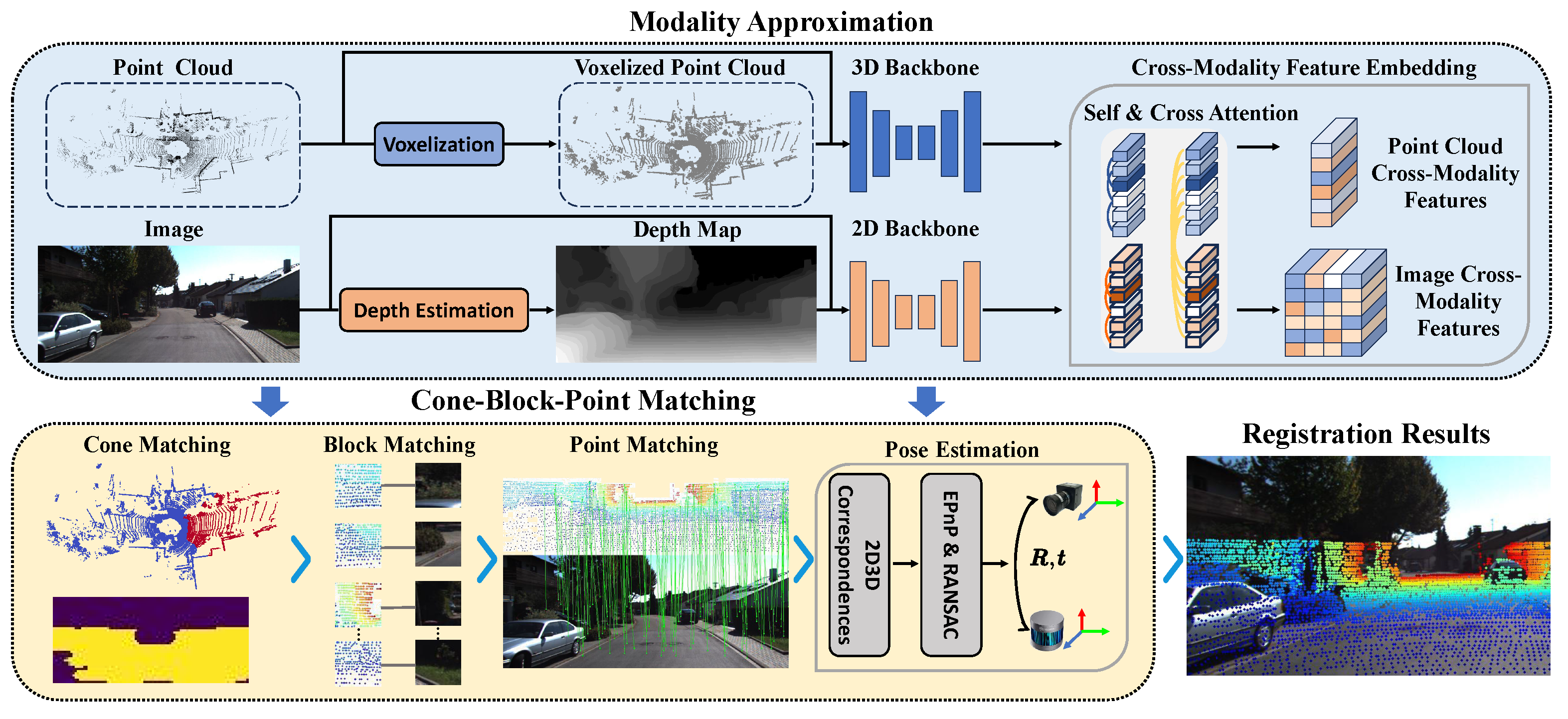
Figure 2 illustrates the overview of our MAC-I2P. In order to achieve accurate 2D–3D correspondences, our MAC-I2P is designed under an “approximation–fusion–matching” architecture. It is composed of a modality approximation module and a cone–block–point matching strategy. The former utilizes image depth estimation and point cloud voxelization to align images and point clouds in terms of geometric structure and feature representation, respectively. Also, it adopts cross-modal feature embedding to enhance feature repeatability. The latter cone–block–point matching establishes pixel-to-point correspondences by leveraging aligned cross-modality features.

3.2. Modality Approximation

Images and point clouds exhibit complementary characteristics in scene representation, as they capture the texture and geometric structures of the scene, respectively. To fully utilize these complementary data, the relative pose between the image and the point cloud needs to be determined. In conditions where the LiDAR and camera cannot be fixed together (e.g., mounted on different robots), such complementarities become a hurdle to registration due to the modality discrepancies between images and point clouds.

To alleviate the modality discrepancies, the existing I2P methods usually rely on feature fusion to align the feature spaces of images and point clouds. However, the misalignment in geometry structures between images and point clouds limits the learning of cross-modality features, and these discrepancies are often ignored. Instead, under our modality approximation module, additional steps of generating pseudo-RGBD images and point cloud voxelization are performed before feature fusion. This module mitigates the modality discrepancies from both geometric structure and feature representation.

Pseudo-RGBD Images Generation. Directly estimating image depth and projecting point clouds onto the image plane are both viable approaches to recovering the geometric structures of the scene indicated by the image. Compared to the latter, the former can generate denser depth values, but its implementation is correspondingly more challenging. Fortunately, the development of monocular depth estimation techniques has made this approach possible. For the first time, it is introduced into the I2P registration. Based on the estimated depth, pseudo-RGBD images are generated. Additionally, adding a depth estimation module that requires training would increase the network’s burden and could even lead to performance degradation. Hence, an off-the-shelf depth estimation model ${\mathcal{F}}_d$ is leveraged to generate pseudo-RGBD images ${\mathbf{I}}_d\in {\mathbb{R}}^{4\times W\times H}$ [42] by,

$${\mathbf{I}}_d={\mathcal{F}}_d\left(\mathbf{I}\right).$$

(2)

Then, pseudo-RGBD features ${\mathbf{F}}_I$ are extracted through a 2D backbone [18] ${\mathcal{F}}_{2D}$,

$${\mathbf{F}}_I={\mathcal{F}}_{2D}\left({\mathbf{I}}_d\right).$$

(3)

Figure 3 illustrates the similarity between image features and point clouds before and after depth estimation. The warmer the color, the higher the probability of a match with the point cloud. It can be seen that with the introduction of depth maps, pseudo-RGBD images are more responsive to point clouds.

Point Cloud Voxelization. Through grid partitioning and aggregation, local features of images can be easily obtained. In contrast, extracting local features from unorganized point clouds is relatively complex. To enhance the repeatability of cross-modality features, we voxelize point clouds to render them a similar data structure as images. In this way, the local feature representation in point clouds can be made similar to image processing. Considering the information loss caused by voxelization, we designed a 3D backbone with two branches, a point branch ${\mathcal{F}}_p$ and a voxel branch ${\mathcal{F}}_v$.

The local and global features of point clouds, denoted by ${\mathbf{F}}_p^{local},{\mathbf{F}}_p^{global}$, respectively, are obtained through the point branch [43],

$${\mathbf{F}}_p^{local},{\mathbf{F}}_p^{global}={\mathcal{F}}_p\left(\mathbf{P}\right).$$

(4)

Additionally, the local features of the voxelized point cloud ${\mathbf{F}}_v$ are extracted by voxel branch [44],

$${\mathbf{F}}_v={\mathcal{F}}_v\left({\mathbf{P}}_v\right),$$

(5)

where ${\mathbf{P}}_v$ resprents the volized point clouds. Figure 3 demonstrates that the introduction of the voxel branch allows the point cloud features to have stronger compatibility with the image, resulting in improved I2P registration performance accordingly.

Cross-Modality Feature Embedding. In order to learn more discriminative cross-modality features, it is necessary to further align the features from different branches. In detail, a symmetric attention-based module is leveraged to fuse these features. The cross-modality features of point clouds ${\tilde{\mathbf{F}}}_P$ can be obtained by,

$$\begin{array}{cc}\hfill {\mathbf{w}}_I& =Softmax\left(\psi ({\mathbf{F}}_I,{\mathbf{F}}_p^{local})\right),\hfill \\ \hfill {\tilde{\mathbf{F}}}_P^{\prime }& =\psi ({\mathbf{w}}_I{\mathbf{F}}_I,{\mathbf{F}}_p^{local},{\mathbf{F}}_p^{global}),\hfill \\ \hfill {\tilde{\mathbf{F}}}_P& =\psi ({\tilde{\mathbf{F}}}_P^{\prime },{\mathbf{F}}_v^{local}),\hfill \end{array}$$

(6)

where $\psi (·)$ is the feature embedding function for point clouds [43], ${\mathbf{w}}_I$ is the feature weights, and ${\tilde{\mathbf{F}}}_P^{\prime }$ is the cross-modality features without voxel-branch results.

In a similar way, the image cross-modality features ${\tilde{\mathbf{F}}}_I$ can be obtained by,

$$\begin{array}{cc}\hfill {\mathbf{w}}_P& =Softmax\left(\xi ({\mathbf{F}}_I,{\mathbf{F}}_p^{local},{\mathbf{F}}_p^{global})\right),\hfill \\ \hfill {\tilde{\mathbf{F}}}_I& =\xi ({\mathbf{F}}_I,{\mathbf{w}}_P{\mathbf{F}}_p^{local},{\mathbf{w}}_P{\mathbf{F}}_p^{global}),\hfill \end{array}$$

(7)

where $\xi$ denotes the feature embedding for images and ${\mathbf{w}}_P$ is the feature weights of point clouds.

3.3. Cone–Block–Point Matching

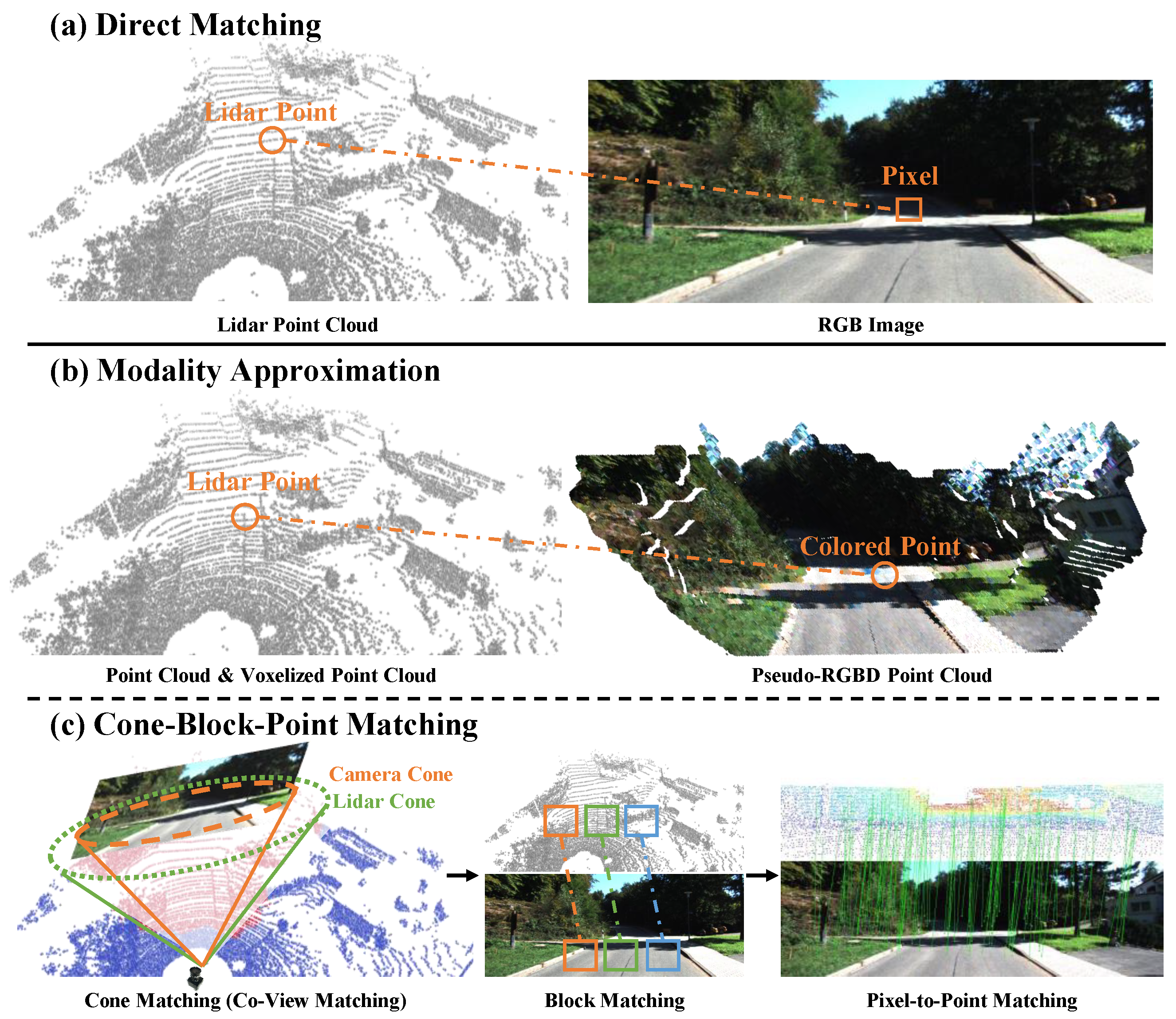
After getting $(\mathbf{I},{\tilde{\mathbf{F}}}_I)$ and $(\mathbf{P},{\tilde{\mathbf{F}}}_P^{\prime },{\tilde{\mathbf{F}}}_P)$, the objective in 2D–3D matching is to establish accurate pixel-to-point correspondences for subsequent pose estimation. Although the cross-modality features with stronger repeatability have been learned, the inter-modality matching between images and point clouds remains non-trivial. On the one hand, the detection angle of a typical LiDAR is 360°, while the field of view of a camera is usually less than 180°. This results in the overlapping observation region between the camera and the LiDAR being cone-shaped, and a significant portion of 3D points can not be observed by the camera. These invisible points are useless matching candidates and are expected to be filtered out. On the other hand, due to the different data densities, establishing one-to-one correspondences between pixels and points is difficult. Therefore, to improve the quality of matching, a cone–block–point matching strategy is proposed and illustrated in Figure 4. It progressively refines the matching scale and relaxes strict matching criteria via multiple weak classifiers, leading to the establishment of accurate pixel-to-point correspondences. Firstly, cone matching is employed to detect the matching cone-shaped region between the camera and the LiDAR. Next, the matching blocks of 3D points and 2D pixels are picked out by block matching. Finally, pixel-to-point correspondences are established based on point matching.

Cone Matching. Due to the sparsity of the point cloud, certain regions corresponding to pixels in the image may not be observed by the LiDAR. Additionally, with the incorporation of semantic and geometric features, regions that possess higher similarity in terms of matching are expected to be selected. Hence, it is essential to identify the matching cone-shaped regions for both the image and the point cloud. To put it into practice, the task of determining the matching cone-shaped region is modeled as the co-view classification for both points and pixels and two co-view classifiers ${\mathrm{CVC}}_{\mathrm{P}}$ and ${\mathrm{CVC}}_{\mathrm{I}}$ for points and pixels are designed, respectively. Considering that this task focuses on the global context, cross-modality features that integrate global characteristics ${\tilde{\mathbf{F}}}_P^{\prime }$ and ${\tilde{\mathbf{F}}}_I$ are used as inputs to ${\mathrm{CVC}}_{\mathrm{P}}$ and ${\mathrm{CVC}}_{\mathrm{I}}$. Then the co-view scores ${\mathbf{S}}_P$ and ${\mathbf{S}}_I$ can be derived as follows:

$${\mathbf{S}}_P={\mathrm{CVC}}_{\mathrm{P}}\left({\tilde{\mathbf{F}}}_P^{\prime }\right),$$

(8)

$${\mathbf{S}}_I={\mathrm{CVC}}_{\mathrm{I}}\left({\tilde{\mathbf{F}}}_I\right).$$

(9)

Based on ${\mathbf{S}}_P\in {\mathbb{R}}^{N\times 1}$ and ${\mathbf{S}}_I\in {\mathbb{R}}^{W\times H}$, co-visible points ${\mathbf{p}}_c$ and pixels ${\mathbf{u}}_c$, along with their cross-modality features ${\tilde{\mathbf{F}}}_P^c$ and ${\tilde{\mathbf{F}}}_I^c$, are identified through thresholds ${\gamma }_P$ and ${\gamma }_I$. Specifically, the point/pixel is considered within the co-view region if the value of ${\mathbf{S}}_P$/${\mathbf{S}}_I$ is greater than ${\gamma }_P$/${\gamma }_I$, respectively.

Two-Dimensional–Three-Dimensional Block Matching. Once the cone matching is performed, it seems possible to establish 2D–3D matches. However, it is important to note that point clouds have absolute scales, while images suffer from scale ambiguity due to perspective projection. This results in the size of the same object appearing to change in the image as the camera moves, while it remains constant in the point cloud. Due to this serious misalignment, the pixel-to-point matching is not a one-to-one correspondence. To overcome such matching ambiguity, an additional step is introduced between cone matching and point matching: generating the matched blocks of points and pixels.

Image blocks and their features $({\mathcal{I}}^{\prime },{\tilde{\mathbf{F}}}_{{\mathcal{I}}^{\prime }})$ can be obtained through grid partitioning, where ${\mathcal{I}}^{\prime }=\left(\{{\mathcal{I}}_1^{\prime },\cdots ,{\mathcal{I}}_{K^{\prime }}^{\prime }|{\mathcal{I}}_{k^{\prime }}^{\prime }\in {\mathbb{R}}^{3\times W^{\prime }\times H^{\prime }})\right\}$. And the generation of point blocks ${\mathcal{P}}^{\prime }$ can be modeled as a classification problem. Specifically, a block classifier ${\mathcal{F}}_{bc}$ is constructed for point clouds using the coordinates of image blocks as labels. With the help of ${\mathcal{F}}_{bc}$, the classification results ${\mathbf{S}}_{P_b}\in {\mathbb{R}}^{N\times K^{\prime }}$ can be obtained,

$${\mathbf{S}}_{P_b}={\mathcal{F}}_{bc}\left({\tilde{\mathbf{F}}}_P\right),$$

(10)

where ${\mathbf{S}}_{P_b}=({[{\mathbf{S}}_{P_{b_1}},\cdots ,{\mathbf{S}}_{P_{b_N}}]}^{\mathrm{T}},{\mathbf{S}}_{P_{b_n}}\in {\mathbb{R}}^{1\times K^{\prime }})$. ${\mathbf{S}}_{P_{b_n}}$ represents the likelihood of a point ${\mathbf{p}}_i\in \mathbf{P}$ matching with each image blocks. The higher the value, the greater the probability of a match. To provide a clearer expression, ${\mathbf{S}}_{P_{b_n}}$ can formulated as follows:

$${\mathbf{S}}_{P_{b_n}}={[S_{{\mathcal{I}}_1^{\prime }},\cdots ,S_{{\mathcal{I}}_{K^{\prime }}^{\prime }}]}^{\mathrm{T}}.$$

(11)

Thus, the image block ${\mathcal{I}}_k^{\prime }\in {\mathcal{I}}^{\prime }$ matched by each point ${\mathbf{p}}_i\in \mathbf{P}$ can be computed by

$$\underset{{\mathcal{I}}_k^{\prime }}{argmax}(S_{{\mathcal{I}}_1^{\prime }},\cdots ,S_{{\mathcal{I}}_{K^{\prime }}^{\prime }}).$$

(12)

In this way, the point blocks that match with the image blocks can be determined and denoted by ${\mathcal{P}}^{\prime }$. Finally, the point blocks with their features are represented by $({\mathcal{P}}^{\prime },{\tilde{\mathbf{F}}}_{{\mathcal{P}}^{\prime }})$.

Dense Pixel-to-Point Correspondences. By utilizing cone matching and block matching, we construct matched point blocks $({\mathcal{P}}^{\prime },{\tilde{\mathbf{F}}}_{{\mathcal{P}}^{\prime }})$ and image blocks $({\mathcal{I}}^{\prime },{\tilde{\mathbf{F}}}_{{\mathcal{I}}^{\prime }})$, and co-visible points $({\mathbf{p}}_c,{\tilde{\mathbf{F}}}_P^c)$ and pixels $({\mathbf{u}}_c,{\tilde{\mathbf{F}}}_I^c)$. To achieve more accurate pose estimation, establishing pixe-to-point matching is necessary. In order to improve the matching quality, the points and pixels that are located in the co-view region and whose blocks are matched are selected. Correspondingly, their features are also picked out. They are represented by $(\mathcal{P},{\tilde{\mathbf{F}}}_{\mathcal{P}})$ and $(\mathcal{I},{\tilde{\mathbf{F}}}_{\mathcal{I}})$, respectively. $(\mathcal{P},{\tilde{\mathbf{F}}}_{\mathcal{P}})$ is the intersection between $({\mathbf{p}}_c,{\tilde{\mathbf{F}}}_P^c)$ and $({\mathcal{P}}^{\prime },{\tilde{\mathbf{F}}}_{{\mathcal{P}}^{\prime }})$. It can be computed by Equation (13),

$$(\mathcal{P},{\tilde{\mathbf{F}}}_{\mathcal{P}})=({\mathcal{P}}^{\prime },{\tilde{\mathbf{F}}}_{{\mathcal{P}}^{\prime }})\cap ({\mathbf{p}}_c,{\tilde{\mathbf{F}}}_P^c),$$

(13)

where $\mathcal{P}=\{{\mathcal{P}}_1,\cdots ,{\mathcal{P}}_V\}$, and V is the number of point blocks. In a similar way, $(\mathcal{I},{\tilde{\mathbf{F}}}_{\mathcal{I}})$ can be obtained by Equation (14),

$$(\mathcal{I},{\tilde{\mathbf{F}}}_{\mathcal{I}})=({\mathcal{I}}^{\prime },{\tilde{\mathbf{F}}}_{{\mathcal{I}}^{\prime }})\cap ({\mathbf{u}}_c,{\tilde{\mathbf{F}}}_I^c),$$

(14)

where $\mathcal{I}=\{{\mathcal{I}}_1,\cdots ,{\mathcal{I}}_K\}$, and the number of matched image blocks is denoted by K.

For any pair of the matched point block ${\mathcal{P}}_v\in \mathcal{P}$ and the image block ${\mathcal{I}}_k\in \mathcal{I}$, the similarity between point ${\mathbf{p}}_i\in {\mathcal{P}}_v$ and pixel ${\mathbf{u}}_j\in {\mathcal{I}}_k$ is defined as the cosine distance between their cross-modality features ${\tilde{\mathbf{F}}}_{p_i}\in {\tilde{\mathbf{F}}}_{{\mathcal{P}}_v}$ and ${\tilde{\mathbf{F}}}_{u_j}\in {\tilde{\mathbf{F}}}_{{\mathcal{I}}_k}$:

$${\delta }^{i,j}=\delta ({\mathbf{p}}_i,{\mathbf{u}}_j)=1-{\displaystyle \frac{{\tilde{\mathbf{F}}}_{p_i}·{\tilde{\mathbf{F}}}_{u_j}}{\parallel {\tilde{\mathbf{F}}}_{p_i}{\parallel }_2·{\parallel {\tilde{\mathbf{F}}}_{u_j}\parallel }_2}}.$$

(15)

Next, the pixel-to-point correspondences of $\{{\mathcal{P}}_v,{\mathcal{I}}_k\}$ can be estimated based on the feature similarity $\delta$, where ${\mathcal{P}}_v=\{{\mathit{p}}_1,\cdots ,{\mathit{p}}_{n_i}\},{\mathcal{I}}_k=\{{\mathit{I}}_1,\cdots ,{\mathit{I}}_{m_i}\}$ ($m_i$/$n_i$ denote the number of pixels/points). The matching between pixels and point clouds is not strictly one-to-one; that is, a pixel may be matched to multiple points. This kind of ambiguous matching can mislead pose optimization. To avoid the ambiguous matching caused by the imbalance in the number of pixels and points, the correspondences ${\mathcal{M}}_{patc{h}^h}$ are determined by finding the point with the largest similarity for each pixel,

$${\mathcal{M}}_{bloc{k}^h}=\left[\begin{array}{c}\left({\mathit{u}}_1,\underset{\mathit{p}\in \{{\mathit{p}}_1,\cdots ,{\mathit{p}}_{n_i}\}}{argmin}\delta ({\mathit{u}}_1,\mathit{p})\right)\\ ⋮\\ \left({\mathit{u}}_{m_i},\underset{\mathit{p}\in \{{\mathit{p}}_1,\cdots ,{\mathit{p}}_{n_i}\}}{argmin}\delta ({\mathit{u}}_{m_i},\mathit{p})\right)\end{array}\right],$$

(16)

where ${\mathrm{block}}^h$ denotes the $h^{th}$ matched blocks. Furthermore, the final 2D–3D correspondences $\mathcal{M}$ can be get by integrating all the $\left\{{\mathcal{M}}_{patc{h}^j}\right|j=1\cdots H\}$,

$$\mathcal{M}=\left[\begin{array}{c}{\mathcal{M}}_{bloc{k}^1}\\ ⋮\\ {\mathcal{M}}_{bloc{k}^h}\\ ⋮\\ {\mathcal{M}}_{bloc{k}^H}\end{array}\right].$$

(17)

With $\mathcal{M}$ and Equation (1), a series of projection equations can be constructed, thereby modeling the I2P registration as a PnP problem. Subsequently, EPnP with RANSAC can be used to optimize the pose iteratively. To provide a more concise and clear explanation of our MAC-I2P’s pose estimating process, the forward inference process of MAC-I2P is presented in Algorithm 1.

Algorithm 1: MAC-I2P inference process

3.4. Loss Function

Our MAC-I2P is trained in a metric learning paradigm. The model is expected to perform cone matching, block matching, and pixel-point similarity estimation simultaneously. Therefore, we design a joint loss function ${\mathcal{L}}_{I2P}$ which consists of the cone matching loss ${\mathcal{L}}_{cm}$, the block matching loss ${\mathcal{L}}_{bm}$, and point matching loss ${\mathcal{L}}_{pm}$.

Cone Matching Loss. After getting ${\mathbf{S}}_P$ and ${\mathbf{S}}_I$, based on the ground truth pose $\mathbf{T}$ and the intrinsic matrix $\mathbf{K}$, the co-view region between $\mathbf{I}$ and $\mathbf{P}$ can be determined. The points and pixels within the co-view region are forced to have higher scores, and vice versa. In order to reduce the computational requirements, H pairs of points and pixels from the co-view region with their scores ${\mathbf{S}}_{P,pos}$ and ${\mathbf{S}}_{I,pos}$ are sampled. Besides, H pairs of pixels and points in the non-overlapping region are also collected and denoted by ${\mathbf{S}}_{P,neg}$ and ${\mathbf{S}}_{I,neg}$. Inspired by CorrI2P [12], the cone matching loss ${\mathcal{L}}_{cm}$ is defined as follows:

$${\mathcal{L}}_{cm}^{in}={\displaystyle \frac{1}{H}}\sum _{h=1}^H((1-{\mathbf{S}}_{P,pos})+(1-{\mathbf{S}}_{I,pos})),$$

(18)

$${\mathcal{L}}_{cm}^{out}={\displaystyle \frac{1}{H}}\sum _{h=1}^H({\mathbf{S}}_{P,neg}+{\mathbf{S}}_{I,neg}),$$

(19)

$${\mathcal{L}}_{cm}={\mathcal{L}}_{cm}^{in}+{\mathcal{L}}_{cm}^{out}.$$

(20)

Block Matching Loss. The block matching between ${\mathcal{P}}_v$ and ${\mathcal{I}}_k$ is formulated as a multi-label classification problem. Based on the image scaling factor s, the intrinsic matrix $\mathbf{K}$, and the ground truth pose $\mathbf{T}$, the matching label ${\mathbf{u}}_g$ for each point ${\mathbf{p}}_i$ can be determined by projecting 3D points onto the image plane,

$${\mathbf{u}}_g={\left[s\mathbf{K}\mathbf{T}{\mathbf{p}}_i\right]}_{:2}.$$

(21)

For brevity, the homogeneous and non-homogeneous transformations in Equation (21) are omitted, and ${[·]}_{:2}$ denotes taking the first two rows of the vector. After obtaining ${\mathbf{u}}_g$, the loss function for this multi-classification problem is defined as the cross-entropy,

$${\mathcal{L}}_{bm}=-{\displaystyle \frac{1}{H}}\sum _{i=1}^H{l}_i\left({\mathbf{p}}_{i,{\mathbf{u}}_g}\right),l_i=-log{\displaystyle \frac{exp\left({\mathbf{p}}_{i,{\mathbf{u}}_g}\right)}{{\displaystyle \sum _{c=1}^C}exp\left({\mathbf{p}}_{i,{\mathbf{u}}_c}\right)}},$$

(22)

where ${\mathbf{p}}_{i,{\mathbf{u}}_c}$ denotes the logit of classifying ${\mathbf{p}}_i$ to ${\mathbf{u}}_c$.

Point Matching Loss. We aim for the feature distance between matching pixel-point pairs to be significantly lower than that of non-matching pairs. Based on the matching ground truth obtained by Equation (21), naturally, a contrastive loss or a triplet loss can be utilized to supervise the model optimization. Furthermore, to enhance the discriminative capacity of the model, we opt for circle loss [45], which possesses a circular decision boundary, for model optimization. Consequently, our matching loss ${\mathcal{L}}_{pm}$ is computed as,

$${\mathcal{L}}_{pm}=log[1+\sum e^{{\mu }_p({\delta }^p-M_p)}·\sum e^{{\mu }_n(M_n-{\delta }^n)}],$$

(23)

where ${\delta }^p$ represents the cosine distance between a matched pair (positive) of points and pixels, while ${\delta }^n$ represents an unmatched one (negative). $M_p$ and $M_n$ are the margins for better similarity separation. The weighting factor for a positive pair is ${\mu }_p=\lambda ({\delta }^p-M_p)$, while for a negative pair is ${\mu }_n=\lambda (M_n-{\delta }^n)$.

Total Loss. After getting ${\mathcal{L}}_{cm}$, ${\mathcal{L}}_{bm}$ and ${\mathcal{L}}_{pm}$, the joint loss ${\mathcal{L}}_{I2P}$ is defined as the weighted sum of these individual loss terms,

$${\mathcal{L}}_{I2P}={\beta }_1{\mathcal{L}}_{cm}+{\beta }_2{\mathcal{L}}_{bm}+{\beta }_3{\mathcal{L}}_{pm},$$

(24)

where ${\beta }_1,{\beta }_2,$ and ${\beta }_3$ are weight coefficients. Based on ${\mathcal{L}}_{I2P}$, our MAC-I2P can simultaneously perform the co-view region detection, the selection of matched 2D–3D blocks, and point-to-pixel matching.

4. Experiments

4.1. Setup

4.1.1. Dataset

Our MAC-I2P underwent evaluation on the KITTI Odometry [13] and Oxford Robotcar [14] datasets, which are both large-scale outdoor benchmarks. To ensure fairness in the experimental setup and generate diverse image-to-point cloud scenes, we followed the same data protocol as previous studies [11,12]. In addition, the registration performance of different methods on self-collected data, which we collected ourselves, was also evaluated.

KITTI Odometry. To ensure overlapping observations, images (obtained by PointGrey Flea2 video cameras) and point clouds (obtained by a Velodyne HDL-64E 3D laser scanner) with the same frame ID were selected. Then 40,960 points were sampled per point cloud and the images were resized to 160 × 512 × 3 to strike a balance between computational efficiency and performance. After that, random translations and rotations were performed for point clouds to avoid network overfitting caused by fixed calibration parameters. They involved translations within a range of 10 m and no limited angle rotations around the up-axis. Besides, the ground truth relative poses were calculated with the inverse transformation. Finally, following the settings of Ren et al. [12] and Li et al. [11], sequences 00 to 08 were used for training, which consisted of a total of 40,818 pairs data. For testing, sequences 09 to 10 were utilized, which provided a total of 5584 pairs.

Oxford Robotcar. Unlike KITTI Odometry, Oxford Robotcar utilized a SICK LMS-151 2D LiDAR to capture the 3D information of the environment. To make the 3D data denser, the point clouds were constructed by accumulating scans from the 2D LiDAR. In detail, each point cloud was defined with a radius of 50 m. As for the generation of image-point cloud pairs, first, a frame of point cloud from one traversal was chosen. Then, an image from the same traversal which was captured within ±10 m from the coordinate origin of the point cloud was randomly selected. After that, a random rotation (around the up-axis) within the same range as KITTI Odometry was applied to the point clouds. For both training and testing, the image was set to $384\times 640$ and the number of points was 40,960. Finally, 109,398 data pairs from 34 traversals were utilized for training purposes, while 13,545 data pairs from 4 traversals were employed for testing.

Self-collected Data. As shown in Figure 7a, a mobile robot equipped with a monocular camera (MV-CA050-12UC) and a LiDAR (Livox Avia) was used to collect images and point cloud data outdoors. In comparison to KITTI Odometry and Oxford Robotcar, the self-collected data exhibited two main characteristics: Firstly, self-collected point clouds possessed higher data density. Secondly, the data collection scenes encompassed a variety of semantic objects such as buildings, signs, and trees. After data collection, the self-collected data was organized using the same data processing method as in KITTI Odometry. The training dataset included 1252 pairs of images and point clouds, while the testing dataset consisted of 314 pairs.

4.1.2. Implementation Details

All the experiments were performed on a workstation equipped with an AMD Ryzen 9 5900X processor (Santa Clara, CA, USA) and an NVIDIA GeForce RTX 3090 GPU (Santa Clara, CA, USA). Our MAC-I2P was implemented using PyTorch 1.12. The Adam optimizer was employed for network training. Our network was trained for 25 epochs on each dataset, with a batch size of 16 for training and 8 for testing. The learning rate of the optimizer was initialized as ${10}^{-3}$ and decayed by 75% every 5 epochs. During training, we set the safe threshold for reprojection error to 1 pixel, and ${\beta }_1={\beta }_3=2,{\beta }_2=1$.

For pose estimation, the co-view thresholds ${\gamma }_P$ and ${\gamma }_I$ were experimentally set, where ${\gamma }_P={\gamma }_I=0.95$. The relative pose was estimated using EPnP under the RANSAC framework. The iterations of RANSAC were set to 5000, with a reprojection error threshold of 1 pixel.

4.1.3. Evaluation Metrics

The performance of image-to-point cloud registration was evaluated with three metrics:

Relative Translation Error (RTE). The relative error in the translation vectors between the predicted pose ${\mathit{t}}_{pred}$ and ground truth pose ${\mathit{t}}_g$ is as follows:

$$\mathrm{RTE}=\parallel {\mathit{t}}_{pred}-{\mathit{t}}_g{\parallel }_2.$$

(25)

Relative Rotation Error (RRE). The predicted and ground truth rotation matrix are denoted by ${\mathit{R}}_{pred}$, ${\mathit{R}}_g$, respectively. Then the relative rotation error between ${\mathit{R}}_{pred}$, ${\mathit{R}}_g$ can be obtained by ${\mathit{R}}_{pred}^{-1}{\mathit{R}}_g$. Following previous studies [11,12], we convert the results of ${\mathit{R}}_{pred}^{-1}{\mathit{R}}_g$ into Euler angle, and the RRE can be calculated as

$$\mathrm{RRE}=\sum _{i=1}^3\left|\theta \left(i\right)\right|,$$

(26)

where $\theta (·)$ denotes the Euler angle of ${\mathit{R}}_{pred}^{-1}{\mathit{R}}_g$, and $\theta \left(1\right)$, $\theta \left(2\right)$, and $\theta \left(3\right)$ are roll, pitch, and yaw, respectively.

Registration Recall (RR). RR is the fraction of successful registrations within the test dataset. A registration is deemed successful if RTE/RRE is smaller than ${\tau }_t/{\tau }_r$. Thus, RR can be defined as follows:

$$\mathrm{RR}={\displaystyle \frac{1}{\tilde{M}}}\sum _{i=1}^{\tilde{M}}[[{\mathrm{RTE}}_i<{\tau }_t\wedge {\mathrm{RRE}}_i<{\tau }_r]],$$

(27)

where $\tilde{M}$ represents the total number of data samples and $[[·]]$ is the Iverson bracket, while ${\mathrm{RTE}}_i$ and ${\mathrm{RRE}}_i$ ($i=1,\cdots ,\tilde{M}$) denote the relative translation and rotation error of the $i^{\mathrm{th}}$ data sample, respectively.

In addition to registration accuracy, the following metrics were adopted to evaluate the matching accuracy of point-to-pixel correspondences:

Inlier Ratio (IR). The fraction of inliers among all putative correspondences. A correspondence is considered an inlier if the distance between the ground truth pixel and the predicted pixel is smaller than a threshold ${\tau }_d$. Then the IR is formulated as

$$\mathrm{IR}={\displaystyle \frac{1}{|\tilde{C}|}}\sum _{({\mathbf{u}}_i,{\mathbf{p}}_i)\in \tilde{C}}[[{\parallel {\mathbf{u}}_i-\pi (\mathbf{K},{\mathbf{T}}_g,{\mathbf{p}}_i)\parallel }_2<{\tau }_d]],$$

(28)

where $\tilde{C}$ is the estimated correspondences set and $|\tilde{C}|$ represents the number of correspondences.

Feature Maching Recall (FMR). FMR refers to the proportion of the test data where the IR is higher than the threshold ${\tau }_m$, which is formulated as

$$\mathrm{FMR}={\displaystyle \frac{1}{\tilde{M}}}\sum _{i=1}^{\tilde{M}}[[{\mathrm{IR}}_i>{\tau }_m]].$$

(29)

4.1.4. Compared Methods

• DeepI2P [11]. DeepI2P utilizes the concept of frustum binary classification to train a classifier that determines whether a given point cloud falls within the camera’s field of view. Based on the classification results, DeepI2P offers two approaches for estimating the relative pose: DeepI2P (2D) and DeepI2P (3D).
• CorrI2P [12]. This approach introduces an attention-based module to fuse image features and point cloud features. It generates cross-modality features for both images and point clouds, allowing the establishment of 2D–3D correspondences. Leveraging these correspondences, the relative pose estimation is performed.
• EFGHNet [33]. This method adopts a divide-and-conquer strategy to separate the tasks of feature alignment and feature matching, enabling independent estimation of each component. The pose estimation is subsequently performed based on the results obtained from feature matching.
• VP2P [9]. VP2P proposes a triplet network to construct a cross-modal feature space between images and point clouds. An end-to-end training strategy is designed based on a differentiable PnP layer. Due to the lack of open-source code and the availability of pre-trained weights for KITTI Odometry, we only evaluated its performance on KITTI Odometry.
• EP2P-Loc [46]. EP2P-Loc introduces image positional encoding to localize matching regions in a coarse-to-fine manner, and optimizes the network through a differentiable PnP layer.
• ${\mathbf{I2P}}_{\mathbf{ppsim}}$ [47]. ${\mathrm{I2P}}_{\mathrm{ppsim}}$ leverages a siamese layer to map 2D and 3D features into an aligned feature space, where 2D–3D correspondences are determined based on feature distances.

4.2. Quantitative Experiments

Registration Accuracy. The registration performance of our MAC-I2P was compared with other state-of-the-art (SOTA) methods, including DeepI2P (3D) [11], DeepI2P (2D) [11], CorrI2P [12], and VP2P [9]. Notably, we purposely deviated from CorrI2P’s way of excluding samples with large registration errors. Instead, the average RTE and RRE for all the samples were evaluated, as in our opinion, this was a more comprehensive way of reporting the performance. For RR, the values of ${\tau }_t$ and ${\tau }_r$ were set to 5 m and $2^{\circ }$, respectively. The quantitative results are provided in

Table 1. Registration accuracy on KITTI Odometry and Oxford Robotcar. The best results are highlighted in bold.

	KITTI Odometry			Oxford Robotcar
	RTE (m) ↓	RRE (°) ↓	RR (%) ↑	RTE (m) ↓	RRE (°) ↓	RR (%) ↑
DeepI2P-3D (CVPR’21) [11]	3.17 ± 3.22	15.52 ± 12.73	3.77	2.27 ± 2.19	15.00 ± 13.64	62.35
DeepI2P-2D (CVPR’21) [11]	3.28 ± 3.09	7.56 ± 7.63	25.95	1.65 ± 1.36	4.14 ± 4.90	69.54
CorrI2P (TCSVT’23) [12]	2.32 ± 9.74	4.66 ± 6.79	72.42	3.20 ± 3.14	2.49 ± 8.51	40.64
EFGHNet (RA-L’22) [33]	4.83 ± 2.92	4.58 ± 8.67	5.65	3.78 ± 3.48	4.76 ± 5.69	20.33
VP2P (NeurIPS’23) [9]	0.75 ± 1.13	3.29 ± 7.99	83.04	-	-	-
EP2P-Loc (ICCV’23) [46]	1.32 ± 1.13	4.11 ± 5.46	-	-	-	-
${\mathrm{I2P}}_{\mathrm{ppsim}}$ (TOMM’24) [47]	1.18 ± 1.48	4.08 ± 4.46	78.49	2.95 ± 2.66	2.26 ± 5.12	52.33
MAC-I2P	0.69 ± 0.86	2.64 ± 2.95	94.94	1.39 ± 1.26	1.53 ± 5.11	78.96

↓ and ↑ indicate that the performance of this indicator is improving.

, from which it can be observed that MAC-I2P achieves superior performance over its competitors on both datasets. Notably, our method outperforms the state-of-the-art (SOTA) by 8.0∼63.2% in RTE and 19.3∼38.5% in RRE. Similar to our approach, both CorrI2P and VP2P establish 2D–3D correspondences through feature matching. However, our method exhibits remarkable superiority over them for two main reasons. First, previous studies overlooked the misaligned geometry structures between images and point clouds, which makes it difficult to learn cross-modal features. Second, they did not adopt a hierarchical matching strategy, which increases the number of matching outliers.

Moreover, our method exhibits more robust performance across both datasets compared to the other methods, whereas CorrI2P and DeepI2P demonstrate inconsistent performance on the two datasets. This inconsistency is mainly attributed to the different point cloud densities. The point clouds in the Oxford Robotcar dataset are relatively sparse, with fewer point cloud observations available for semantic objects such as cars and pedestrians. Consequently, extracting meaningful semantic features from the point clouds becomes more challenging. This factor leads to a decline in registration performance for CorrI2P, which relies on pixel-to-point matching and struggles to capture the semantic objects in the scene. In contrast, our method leverages modal approximation and cone–block–point matching to mitigate modality discrepancies and reduce outliers, thereby demonstrating superior registration robustness.

In addition, the registration accuracy evaluation results of the different methods on the self-collected data are also provided in

Table 2. Quantitative results of registration accuracy on self-collected data. The best results are highlighted in bold.

	RTE (m) ↓	RRE (°) ↓
CorrI2P [12]	3.28 ± 6.10	4.88 ± 9.79
VP2P [9]	3.25 ± 5.88	6.18 ± 11.06
MAC-I2P	1.26 ± 1.95	3.22 ± 4.78

↓ indicates that the performance of this indicator is improving.

. The results from Table 2 indicate that our MAC-I2P outperforms other competitors in terms of registration accuracy.

Point-to-Pixel Correspondence. Apart from registration performance, a quantitative evaluation of the methods’ cross-modal feature learning capabilities was also conducted. Since the quality of establishing 2D–3D correspondences is directly linked to the effectiveness of cross-modal representation, IR and FMR were employed to compare the abilities of the different methods in establishing 2D–3D correspondences. The quantitative results are provided in

Table 3. Quantitative results of point-to-pixel correspondences on KITTI Odometry. The best results are highlighted in bold. Here, we report the IR (%)/FMR (%) with different thresholds ${\tau }_d$(pixel)/${\tau }_m(\%)$.

	${\mathbf{IR}}_1$/${\mathbf{FMR}}_{0.2}$ ↑	${\mathbf{IR}}_2$/${\mathbf{FMR}}_{0.2}$ ↑	${\mathbf{IR}}_3$/${\mathbf{FMR}}_{0.2}$ ↑
CorrI2P [12]	10.84/18.12	27.69/64.60	42.18/82.38
VP2P [9]	21.23/68.49	44.39/96.54	69.95/97.87
MAC-I2P	37.60/83.81	59.26/97.04	71.34/99.61

↑ indicates that the performance of this indicator is improving.

, where we set ${\tau }_d=1,2,3$, ${\tau }_m=0.2$ and denote them by ${\mathrm{IR}}_d$ and ${\mathrm{FMR}}_m$, respectively. By comparing the results, it can be seen that our method achieves the optimal results in terms of both IR and FMR across various threshold settings. Notably, our MAC-I2P outperforms CorrI2P and VP2P by a margin of 69.13∼246.86% and 1.94∼77.10%, respectively, in terms of IR.

Registration Robustness. Typically, the time to acquire a frame of data by the LiDAR is longer than the exposure time of the camera. Thus, there can indeed be slight offsets in the point cloud of moving objects in the scene. This can lead to outlier matching and consequently affect registration performance. In order to analyze the effect of point offset on I2P registration, additional comparative experiments were carried out. In detail, by applying a random offset to each coordinate of the point cloud, point offset was simulated on KITTI Odometry. Next, different methods were evaluated on the dataset with random offset. The results in

Table 4. Quantitative results of registration accuracy on KITTI Odometry with random offset. The best results are highlighted in bold.

	RTE (m) ↓	RRE (°) ↓
CorrI2P [12]	2.95 ± 3.62	5.29 ± 9.81
VP2P [9]	1.06 ± 1.78	3.43 ± 6.55
MAC-I2P	0.79 ± 1.02	2.90 ± 3.80

↓ indicates that the performance of this indicator is improving.

show that our MAC-I2P outperforms significantly compared to other methods. This is mainly attributed to two factors. First, the proposed cone–block–point matching deconstructs 2D–3D matching into three hierarchical matching tasks: region-to-region, block-to-block, and pixel-to-point matching. Among these tasks, the first two focus more on scene semantic information, hence being insensitive to point offsets. Point matching is considered valid only if both the region matching and the block matching to which the pixel and point belong are successful. Therefore, the issue of point offsets can be alleviated through cone–block–point matching. Second, MAC-I2P utilizes the PnP with RANSAC to estimate poses, effectively removing outliers caused by point offsets.

Generalization Capability. The generalization capability evaluation results are presented in

Table 5. The cross-dataset evaluation performance and the registration accuracy under different data partitioning ways on KITTI Odometry. MAC-I2P (i,j) signifies that MAC-I2P uses the former i sequences as the training set and the subsequent j sequences as the testing set. “KITTI Odometry → Oxford Robotcar” signifies that the model is trained on KITTI Odometry, fine-tuned and tested on Oxford Robotcar, and vice versa.

	RTE (m) ↓	RRE (°) ↓
KITTI Odometry
MACI-2P (7,4)	0.77 ± 0.99	2.70 ± 3.20
MACI-2P (8,3)	0.72 ± 0.81	2.67 ± 3.04
MAC-I2P (9,2)	0.69 ± 0.86	2.64 ± 2.95
KITTI Odometry → Oxford Robotcar
DeepI2P [11]	3.01 ± 7.36	6.14 ± 9.84
CorrI2P [12]	4.10 ± 6.52	4.58 ± 9.31
MAC-I2P	1.54 ± 2.05	1.63 ± 4.93
Oxford Robotcar → KITTI Odometry
DeepI2P [11]	5.48 ± 12.44	9.20 ± 14.33
CorrI2P [12]	3.41 ± 8.56	5.65 ± 7.60
MAC-I2P	1.02 ± 2.73	4.48 ± 7.46

↓ indicates that the performance of this indicator is improving.

. First, the impact of different dataset partitioning methods on the performance of MAC-I2P was analyzed. As indicated in Table 5, reducing the size of the training set does lead to a decrease in registration accuracy, but such a decrease is not substantial. Meanwhile, even with a reduced training set, our MAC-I2P still achieves SOTA.

Second, cross-dataset experiments were conducted to provide a comprehensive analysis of the generalization capabilities of our MAC-I2P. Specifically, we transferred the model trained on KITTI Odometry to Oxford Robotcar and evaluated the model’s registration performance on the testing set of Oxford Robotcar. Similarly, we obtained results for transferring from Oxford Robotcar to KITTI Odometry. The relevant experimental results are shown in Table 5. It can be seen that MAC-I2P still outperforms its competitors significantly. This is mainly due to the generation of pseudo-RGBD images in our modality approximation scheme and the proposed cone–block–point matching strategy. The former does not require retraining for specific scenarios, while the latter provides additional weakly supervised information for the model of MAC-I2P. Therefore, our MAC-I2P exhibits a strong generalization ability.

Runtime and GPU Memory Usage The pose inference time and GPU memory usage of different I2P registration methods were compared, and the quantitative results are reported in

Table 6. Runtime and GPU memory usage.

	Pose Infer. (s) ↓	GPU Mem. (MB) ↓
DeepI2P (3D) [11]	39.39	2906
DeepI2P (2D) [11]	26.01	2906
CorrI2P [12]	9.86	3208
VP2P-Match [9]	0.31	17,169
MAC-I2P (Ours)	0.33	9832

↓ indicates that the performance of this indicator is improving.

. It can be seen that MAC-I2P attains a favorable balance between runtime and memory usage. By contrast, DeepI2P tends to produce ambiguous 2D–3D correspondences and requires a time-consuming inverse camera-projection procedure for pose optimization; CorrI2P is encumbered by a large set of externally matched points, inflating the cost of iterative refinement; and VP2P-Match relies on a transformer-based 3D backbone, which imposes substantial GPU memory demands.

4.3. Qualitative Experiments

Visual Comparison of Registration on KITTI Odometry. The visualization results of different methods on the KITTI Odometry dataset are shown in Figure 5. To make the visualization more intuitive, the point clouds were projected onto the image planes based on the predicted relative poses, and the corresponding RTEs and RREs were annotated. The color of each point indicates its distance from the camera. It can be observed that our method achieves better registration results compared to the other methods, particularly in road scenes with different translational and rotational perturbations. In scenes with elongated structures or sparse semantic objects (e.g., the first and fourth rows), DeepI2P, CorrI2P, and VP2P struggle to estimate satisfactory relative poses, resulting in significant misalignments of trees or cars.

Visual Comparison of Registration on Oxford Robotcar. The visual results of different approaches on Oxford Robotcar are presented in Figure 6 in the same way as employed in KITTI Odometry. Although multi-frame accumulation was performed, the point clouds in Oxford Robotcar were still relatively sparse, which made I2P registration more challenging. It can be seen that our method demonstrates significantly superior registration performance in different road scenes compared to DeepI2P and CorrI2P. This further confirms that our method is not sensitive to point cloud density and can be adapted to a wider range of application scenarios.

Visual Comparison of Registration on Self-collected Data. The visual registration comparison between our method and other competitors was carried out on the self-collected data, and the results are illustrated in Figure 7b. From Figure 7b, it can be obviously observed that neither CorrI2P nor VP2P can effectively align the images and point clouds. By contrast, our MAC-I2P can align images and point clouds more accurately, which is attributed to its pseudo-RGBD image generation and cone–block–point matching.

4.4. Ablation Study

Components. To validate the effectiveness of different components, ablation experiments were conducted on the KITTI Odometry dataset, and the results are reported in Table 7. The components examined in our ablation study are elaborated as follows:

• DE: Depth estimation module for images;
• VB: Voxel branch for point clouds;
• CBP: Cone–block–point matching for establishing 2D–3D correspondences.

We replaced the cone–block–point matching (CBP) with the feature matching method adopted in CorrI2P [12]. The effectiveness of CBP is illustrated in the 4th and last rows. We removed the voxel branch (VB) from the modality approximation module, which means that the cross-modal feature fusion stage only utilized the point branch features of the point cloud. The effectiveness of VB can be confirmed by comparing the 2nd and 4th rows. Similarly, we removed the image depth estimation module (DE) from the modality approximation scheme, which means that the 2D backbone only extracted features from RGB images. The 1st and 2nd rows of Table 7 demonstrate the effectiveness of introducing the image depth estimation module. Furthermore, the benefits of the modality approximation module for I2P registration can be demonstrated when comparing the data in the 1st and 4th rows of the table.

Table 7. Ablation studies of the components in MAC-I2P. The best results are highlighted in bold.

DE	VB	CBP	RTE (m)	RRE (°)
			1.18 ± 1.48	4.08 ± 4.46
✔			0.92 ± 1.34	3.08 ± 4.42
✔		✔	0.84 ± 1.19	2.90 ± 5.87
✔	✔		0.78 ± 1.35	3.19 ± 7.56
✔	✔	✔	0.69 ± 0.86	2.64 ± 2.95

Table 7. Ablation studies of the components in MAC-I2P. The best results are highlighted in bold.

DE	VB	CBP	RTE (m)	RRE (°)
			1.18 ± 1.48	4.08 ± 4.46
✔			0.92 ± 1.34	3.08 ± 4.42
✔		✔	0.84 ± 1.19	2.90 ± 5.87
✔	✔		0.78 ± 1.35	3.19 ± 7.56
✔	✔	✔	0.69 ± 0.86	2.64 ± 2.95

Robustness to depth map quality: To promote robustness to depth map quality, we augmented training depth maps with controlled perturbations—including Gaussian noise, blur, brightness/contrast shifts, global scale/offset bias, and random holes. Dedicated depth–sensitivity studies were conducted (see

Table 8. Depth–sensitivity analysis on KITTI Odometry.

	RTE (m) ↓	RRE (°) ↓
MAC-I2P	0.69 ± 0.86	2.64 ± 2.95
MAC-I2P(dp)	0.72 ± 0.90	2.71 ± 3.02

↓ indicates that the performance of this indicator is improving.

). In this analysis, MAC-I2P(dp) denotes evaluation with perturbations applied to the depth maps. The results indicate that degraded depth modestly reduces registration accuracy, but the overall impact is moderate, and MAC-I2P remains stable across a wide range of degradation levels. This further underscores the cone–block–point matching framework’s outlier-rejection capability against spurious correspondences.

5. Conclusions

In this paper, we thoroughly investigate the current methods for I2P registration and identify two main challenges that hinder the resolution of this problem: poor repeatable cross-modal feature extraction due to modality discrepancies and low-quality point-to-pixel matching caused by the differences in sensing range and data density. To address these challenges, we propose a novel I2P registration framework called MAC-I2P. MAC-I2P effectively mitigates the modality differences by bringing the two modalities closer through image depth estimation and point cloud voxelization. Furthermore, a cone–block–point matching strategy is proposed, which enhances the quality of 2D–3D correspondences. Extensive experiments demonstrate that MAC-I2P achieves superior registration performance compared to its competitors. Our proposed method not only contributes to the development of I2P registration but also paves the way for other applications involving multi-modal data attributes. It needs to be noticed that although our algorithm strikes a balance between runtime and GPU memory usage, it still demands GPU assistance, and deploying it on resource-constrained edge devices remains challenging. This will be a focus of our future work.