Article

Application of FEM Analyses and Neural Networks Approach in Multi-Stage Optimisation of Notched Steel Structures Subjected to Fatigue Loadings

Department of Machine Design and Composite Structures, Faculty of Mechanical Engineering, Cracow University of Technology, ul. Warszawska 24, 31-155 Cracow, Poland
*
Author to whom correspondence should be addressed.
Appl. Sci. 2025, 15(20), 11194; https://doi.org/10.3390/app152011194
Submission received: 15 September 2025 / Revised: 6 October 2025 / Accepted: 16 October 2025 / Published: 19 October 2025

Abstract

The stress concentration, which appears in loaded structural elements with voids, holes or undercuts, is the main source of premature fatigue failure. So, an increase in fatigue life can be achieved by reducing stress concentrations around the notches. Different techniques can be used to reduce the stress concentration. One of them is the application of additional stress relief undercuts or holes, while a second one relies on the application of overlays glued in the vicinity of notches. The proposed study is focused on the optimisation of notched specimens using a multi-stage optimisation process, including the use of artificial neural networks (ANNs). On this basis, the comparison of the effectiveness of various modern finite element optimisation tools is made. Here, special attention is paid to samples with elliptical holes and the application of the ANN technique in determining the optimal solution for the configuration of stress relief holes. The proposed study is illustrated by the example of a steel specimen with an elliptical opening. Specimens without stress relief holes and with an optimal configuration of stress relief holes are subjected to fatigue tests to confirm the effectiveness of the proposed approach. The performed study revealed that the cutting of additional circular stress relief holes reduces the stress concentration around the elliptical opening by about 12% and leads to an increase in fatigue life by about 79% for the applied material. Moreover, the comparison of the possibilities of the reduction in SCF by the application of stress relief holes, composite overlays and the simultaneous application of composite overlays and stress relief holes for the investigated notched samples is performed. Following the numerical results, it is observed that the use of composite overlays additionally decreases the stress concentration factor in relation to specimens with stress relief holes by an additional 6%.

1. Introduction

Flat structural elements are commonly used in many practical applications. These can be found in the power engineering, automotive or aerospace industries, which are their typical areas of application. In many cases, these elements are subjected to cyclically varying loads. These varying loads lead to the gradual development of micro-damages, which nucleate into cracks and result in premature failure of the whole element. This effect appears for loads below the material’s yield strength or the value of permissible stress commonly used in static analyses. Such a phenomenon is called fatigue failure and plays a key role in structural destruction, causing big economic losses. Holes or voids of different shapes are often made in such elements for assembly, technological or functional reasons. The change in the cross-section of the loaded structure causes the appearance of a stress concentration around the cut void, and the affected area is called the notch area. The local stress increase even can be several times greater than the nominal stress calculated by means of common formulas.
The topic of stress concentration has been the subject of research for over 100 years and was pioneered by Kirsch [1] and Inglis [2]. These researchers, for the first time, elaborated a complete mathematical formulation describing the phenomenon of stress concentration in isotropic plates with circular and elliptical holes. Over the following years, analytical methods describing stresses around notches continued to be developed for both isotropic and anisotropic materials and for different shapes of notches. Based on the theory of elasticity and the strength of materials applied in analytical methods, the determination of mathematical functions describing the stress concentration effect has become accessible. These functions relate quantities like external loads, internal forces and strain. Numerous experiments were also conducted to derive empirical formulas for the determination of the stress concentration factor around typical notches. The results of these studies were published in many books and engineering guides. In particular, the books in [3,4] have proven their efficacy and are still very helpful in engineering practice. Following this approach, determining the stress concentration factor (SCF) requires only knowledge about the kind of notch and the geometric dimensions of the investigated element, as well as material properties and the kind of load applied. Of course, the basic formulas for SCF are set for simple load cases. The assessment of the stress concentration becomes more challenging in the case of complex applied loadings. In such situations, the use of approximate numerical methods can be the remedy. In this area, the finite element method (FEM) is the most commonly used application to determine the stress distribution and stress concentration. Numerous commercial software packages are available for this purpose. The advantage of this method is the rapid acquisition of approximated results for various load cases and arbitrary notch shapes. If there is a necessity for a void application, then circular holes are usually applied in structures. They occur in elements connected with screws, rivets or pins. Methods for determining stress concentrations around a circular hole in a plate under tension have been the subject of numerous studies, both in steel plates [5,6] and composite materials [7,8]. Elliptical holes can be a certain alternative to circular holes. Such a modification introduces additional free parameters like the ratio between semi-axes and the angle of the ellipse orientation with respect to the applied load. In this area, numerous studies with varying half-axis length ratios have also been performed. The basic conclusion is that ellipses with a longer half-axis positioned perpendicularly to the applied load are not an optimal solution due to the significant increase in stress and the reduction in the plate cross-section. Research conducted by Zhong Hu et al. [9] demonstrates a five-fold increase in stresses in the notch for an ellipse whose semi-axis ratio is set to 2. Additionally, the effect of its orientation (angle of the major semi-axis) on the stress concentration was studied for an elliptical hole [10]. The optimal solution is to position the ellipse so that its longer semi-axis overlaps the load direction. Analytical and numerical studies were also conducted for holes with regular shapes such as triangles, squares or regular pentagons. The effect of the notch shape and its orientation on the stress concentration factor was described. For a rectangular notch with rounded corners, a lower stress concentration was obtained than for other holes, including circular holes [11,12].
Further decreases in the stress concentration and corresponding increases in fatigue life can be obtained through the reinforcement of notched structures using composite overlays. These should be applied in the vicinity of the considered notch. Such an approach results in an increase in fatigue life within the range 20–890% [13,14,15,16]. Such an increase is provided mainly by the adhesive properties and their chemical composition.
Numerical strength analyses based on the finite element method, although accurate, are often time-consuming and require significant computational efforts. Therefore, mechanical engineering is increasingly employing modern computational methods such as machine learning. In this area, the artificial neural network (ANN) approach is of the utmost importance. These methods allow for quick and precise prediction of material behaviour under applied loads. A sufficient amount of input data, which typically comes from experiments or FEM analysis, is essential for accurate analysis results. Machine learning is used to predict stresses around notches such as circular holes [17], V-notches [18], fillets [19] and welded joints [20]. Hou et al. [21] developed a generalised regression neural network algorithm for predicting stresses around a central circular hole in a composite plate under tension. They also extended their algorithm to include two holes but with the restriction that the holes had a constant diameter or a constant distance from the centre of the sample. On the other hand, reference [22] presented a probabilistic neural network model for predicting the tensile strength of composite plates with an open hole using a limited number of experimental input data. The prediction error did not exceed 9%, which is satisfactory in view of the small amount of input data. Rezasefat et al. [23] presented a machine learning surrogate model for predicting the stress distribution around an arbitrary-shaped hole. The input data, in the form of a stress array, was derived from FEM simulations and then fed into a convolutional neural network model. The study showed that satisfactory results were obtained only for holes whose shape had previously been used in neural network training. After using a different shape, the prediction accuracy decreased. Similarly, for the number of holes, if the model was trained with one hole and then two holes were introduced, the error exceeded 20%. These results demonstrate the importance of appropriately selecting the training set for the neural network. However, Zhang et al. [24] developed an ANN model to predict progressive damage in a CFRP laminate with a round hole. The results show that the ANN model can effectively predict damage propagation, and the model’s prediction accuracy can be improved by appropriately selecting the structural parameters of the neural network.
The application of time-varying loads causes a challenge for designers who must determine the fatigue life of such structures. This is not an easy task due to the nonlinearity of the failure effect and the multitude of factors influencing material fatigue. Using machine learning algorithms, fatigue life can be predicted with good accuracy, as demonstrated by numerous publications. Marković et al. [25] developed a surrogate artificial neural network model trained on data from FEM simulations to estimate the fatigue life of steel elements with notches. The results show that higher accuracy was achieved for low-cycle fatigue, where over 87% of predictions fell within the specified range. Similar studies were also performed for titanium alloy structural parts with various notches using a genetically optimised backpropagation artificial neural network [26]. Each neural network had its own parameters, such as the number of hidden layers, the number of neurons and activation functions, which influenced the obtained analysis results. The influence on the estimation of low-cycle fatigue parameters was investigated [27], and the optimal ANN structure was determined based on this. Using neural networks, fatigue life under step loading [28] and welded structures [29] was estimated in real time [30]. In industry, the assessment of fatigue crack propagation occurring in important structures is an important aspect. Using machine learning algorithms, fatigue crack growth can be predicted [31,32]. Zhang et al. [33] proposed a Gaussian Variational Bayes Network probabilistic prediction model for fatigue life evaluation for a limited size of input data (100–300 samples). They observed significant improvements in the R2 parameter for datasets with at least 250 samples.
Due to the fact that various types of composite materials are increasingly used in modern structures, the problem of the influence of all types of openings on the stress distribution around them is still relevant. The stress concentration factor around a circular hole in the case of a flat plate made of a functionally graded material, where both Young’s modulus and Poisson’s ratio vary in the radial direction, is analysed by Mohammadi et al. [34]. The plate is subjected to uniform biaxial tension and pure shear. A general form for the stress concentration factor in the case of biaxial tension is presented. Using a Frobenius series solution, the stress concentration factor is calculated for the pure shear case. The effect of nonhomogeneous stiffness and varying Poisson’s ratio upon the stress concentration factors is analysed. Next, methods for the mitigation of the stress concentration factor in the case of different holes in the plates made of different materials are discussed in the review by Nagpal et al. [35]. In this work, an attempt has been made to present the widest possible range of various techniques and approaches to deal with this task. Monti [36] proposes an original method by the application of a particular porous pattern in order to modify the local stress field and reduce the stress concentration value near the hole boundary. This pattern can be obtained by laser cutting with the appropriate finishing requirements. Picelli et al. [37] present a level set topology optimisation method for the manipulation of stress and strain integral functions in a prescribed region of a linear elastic domain. The method can deviate or concentrate the flux of stress in the sub-structure by optimising the shape and topologies of the boundaries outside of that region. A similar approach has been studied in the problem of pressure vessels subjected to internal pressure and closed by means of flat ends, including stress relief grooves [38]. Wang et al. [39] studied the stress distribution of a functionally graded panel with a central elliptical hole under uniaxial tensile load. Functionally graded material can optimise the mechanical properties of composites by designing the spatial variation in material properties. Based on the inhomogeneity variation and three different gradient directions, the effects of the inhomogeneity on the stress concentration factor and damage factor are discussed. Almeida et al. [40] performed a numerical and experimental investigation on the unnotched and open-hole tensile characteristics of fibre-steered variable-axial, also known as variable-angle-tow and variable-stiffness, composite laminates. They used the digital image correlation (DIC) to accurately capture the strain and failure behaviour. A progressive damage model was then developed to simulate the experimental observations. Yan et al. [41] developed an effective integrated design optimisation method to reduce the maximum von Mises stress around vent holes of a high-pressure turbine sealing disk. It mainly includes four different shape designs (circular, elliptical, race-track and four-arc) for holes, an updated self-developed modelling and meshing tool, a strength analysis and a self-proposed efficient switching delayed particle swarm optimisation algorithm. Recently, FEM has become an essential tool in engineering designing and analysis and usually ensures possibilities to find an optimal configuration of the considered structure [42]. However, if possible, the results obtained in these analyses should be verified by experimental tests.
Based on the above literature review, it can be seen that the use of currently available tools and software offers new possibilities for increasing fatigue life. This work focuses on minimising SCF in elliptically notched elements. Analyses were performed using various tools, both FEM and ANN. A particular focus was the use of ANN. Such a study allowed for the comparison and evaluation of the capabilities of applied methods and software. The first novelty of this work is the optimisation of notched specimens using ANN (as a complementary surrogate tool for FEM) and the comparison of the effectiveness of various modern optimisation tools. Here, special attention is paid to the application of the ANN technique in the determination of the optimal solution. The second novelty relies on the comparison of the possibilities of the reduction in SCF by the application of stress relief holes, composite overlays and the simultaneous application of composite overlays and stress relief holes for the investigated notched samples. According to the authors’ knowledge, similar studies have not been published yet.
The paper consists of seven sections. The extended introduction, including the literature review, is provided in Section 1. The materials and optimisation methodologies are described in Section 2. The results of the performed numerical FEM optimisation studies (Ansys APDL 2024 R2 and Ansys Workbench 2025 R1) are presented in Section 3. The results of optimisation by means of ANN approaches are given in Section 4. These studies are performed for specimens with a single circular opening, a single elliptical opening and an elliptical opening with two stress relief circular holes. The results of the fatigue experimental tests are reported in Section 5. Here, also, the results of FEM calculations for specimens reinforced by composite overlays are presented. A discussion of the obtained results is given in Section 6, and finally, conclusions are provided in Section 7.

2. Materials and Methods

2.1. Experimental Procedures

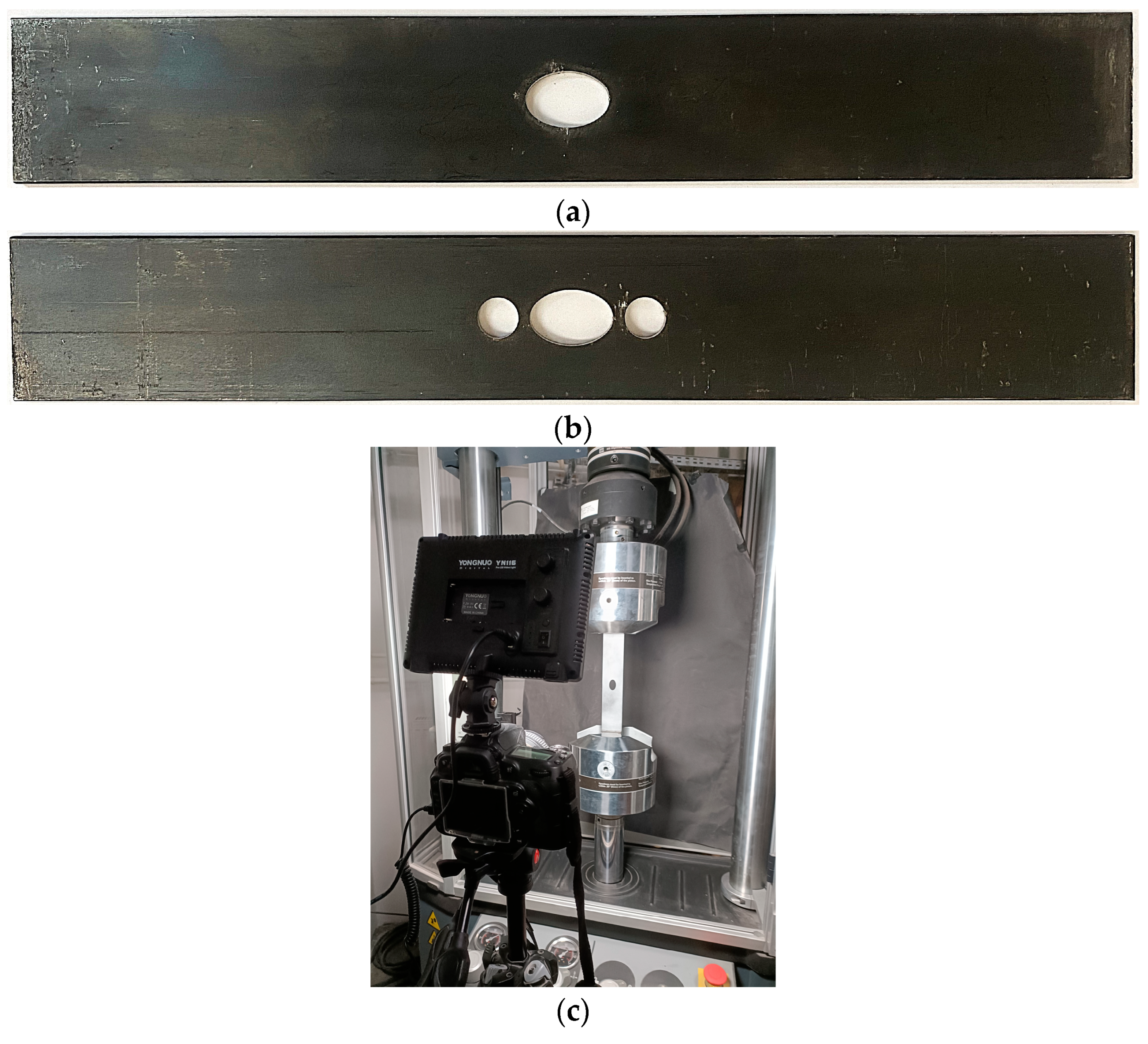
The experimental fatigue tests were conducted on two different sets of samples (each set had three samples). The specimens with a thickness of 4 mm were made of S235JR steel, with the chemical composition listed in Table 1 and mechanical properties shown in Table 2. The geometries of the samples are presented in Figure 1. The first set included steel samples with a single elliptical opening placed in the centre (Figure 1a). In the second set, the two circular relief holes were added (Figure 1b). The configuration of the stress relief holes was determined based on the performed multi-stage optimisation. The openings were cut using laser cutting technology.
Fatigue tests were performed under the same load conditions. The stress ratio was assumed to be R = 0.1. The maximal value of the fatigue tensile loading was set to FMAX = 47 kN. This corresponded to a nominal stress in the weakened cross-section equal to σnom = 392 MPa. The experiments were performed using the MTS Landmark 370 servo-hydraulic test system (Figure 2c). The fatigue loading was applied in a sinusoidal waveform with a frequency equal to 20 Hz. The list of the tested specimens is shown in Table 3. Exemplary photographs of the tested specimens are presented in Figure 2. Additionally, the FEM analyses were carried out for specimens reinforced by composite overlays. It was assumed that the composites were glued on both sides of the steel core, as shown in Figure 1d. The details concerning the preparation of the specimens with composite overlays and adhesive joints are described in previous studies by the authors [13,15]. During preparation of these samples with adhesive joints, special attention should be paid while removing the dust and grease from the surfaces, gluing it with appropriate holders (in order to provide constant adhesive thickness along the whole joint) and seasoning (usually for a minimum of 7 days).

2.2. Finite Element Analyses

2.2.1. Ansys APDL Approaches

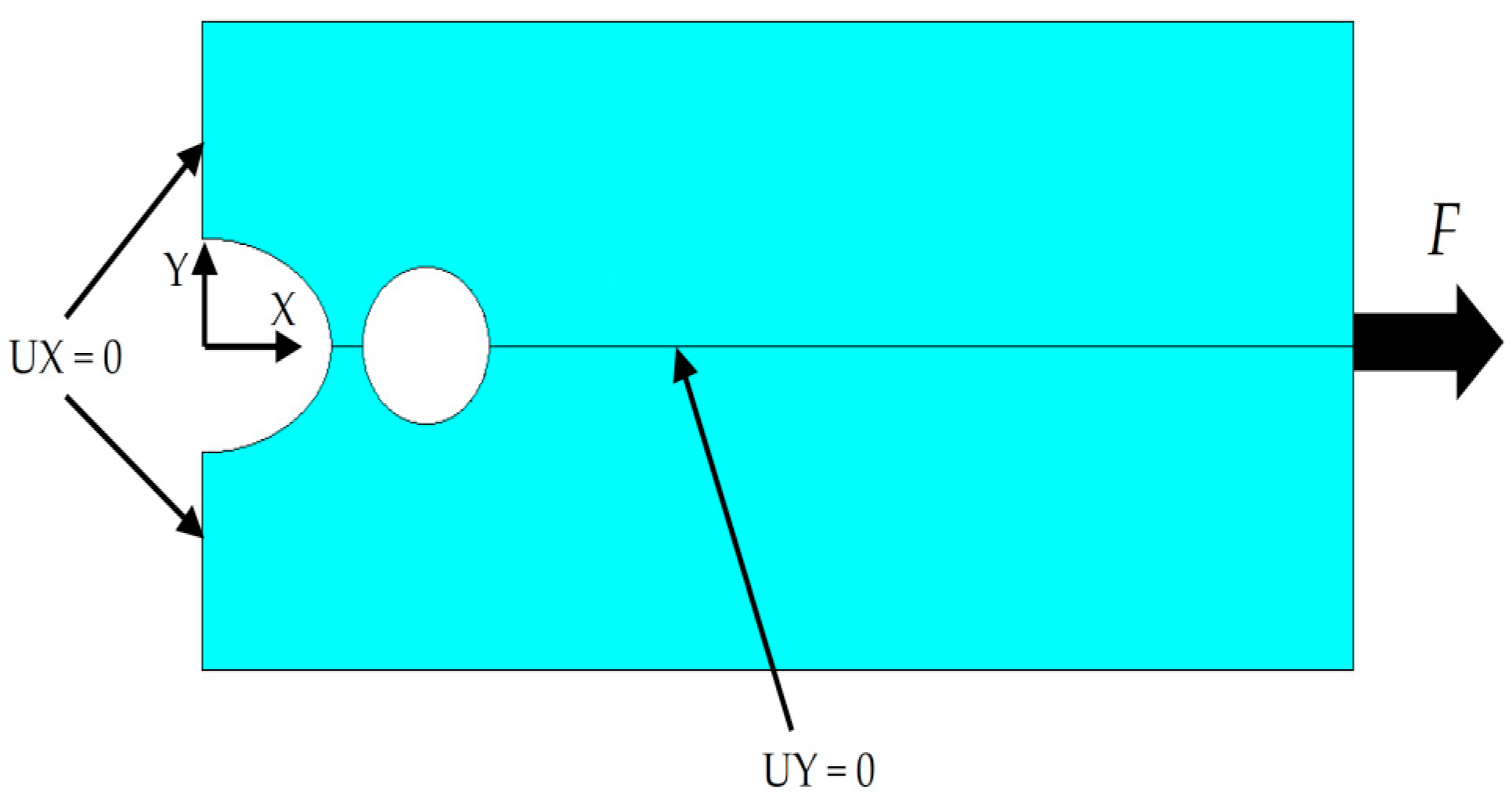
The effectiveness of the applied stress relief holes was analysed numerically by means of the finite element method (FEM). For that purpose, the finite element software Ansys APDL 2024 R2 [45] was used. In the performed studies, static analyses were conducted for samples loaded with tension force F (see Figure 3). The value of the force was set so that the nominal stress values in the cross-section weakened by the elliptical opening were equal to σnom,x = 1 MPa. This approach made it so that the stress σx was also directly equal to the stress concentration factor (Ktn) around the elliptical hole. The two circular stress relief openings were applied. These were located along the sample tension direction and symmetrically placed with respect to the midpoint of the investigated element (see Figure 1). Due to the symmetry, only half of the specimen was numerically investigated. The applied boundary conditions are shown in Figure 3—UY = 0 for all nodes located at y = 0 and UX = 0 for all nodes located at x = 0. In the case of the 3D approach, additionally, the displacement in the z direction was blocked in all mid-plane nodes.
The main aim of the performed numerical studies was to set optimal values of the parameters like the radius of the circle (r) and its position with respect to the elliptical opening (see Figure 1c). Such a position can be described in two ways: as the smallest thickness between an elliptical and circular hole (LW) or the distance between the axes of circular and elliptical openings (LC). The preliminary numerical tests revealed a weak dependency of the Ktn value within certain arbitrarily chosen ranges of parameters. This observation pointed out that a certain risk of getting stuck in a local optimum existed. So, the full numerical analysis was performed following three paths, as follows:
  • Simple search method (SSM) with a gradual narrowing of the search area, Ansys APDL;
  • Ansys parametric optimisation (APO), Ansys APDL;
  • Goal-driven optimisation (GDO), Ansys Workbench.
The detailed analyses were performed for the following geometrical parameters:
  • Plate width W = 45 mm;
  • Semi-axis of the elliptical hole perpendicular to tensile loading direction—a = 0.167/W = 7.5 mm;
  • Second semi-axis of elliptical hole—b = 1.5a = 0.25/W = 11.25 mm.
SSM is time-consuming but a very effective approach, which helps to avoid the stacking of the search solution in a local minimum. The method is easy to illustrate in the case when only two independent variables are considered and the investigated Ktn value can be shown in the form of a surface Ktn = f(r, LW). For the purposes of the analysis, the initial constraints were set as follows:
0.1 W 2 r 0.9 W 0.2   m m L W 5   m m L C =   b + r + L W .
The APO was performed by means of a combination of two optimisation techniques, i.e., the gradient-free zero-order optimisation method (ZOOM) and a gradient-based first-order optimisation method (FOOM). The above-mentioned procedures were activated using the OPSUBP and OPFRST commands, respectively. More details about both procedures are described in Section 3.
In this study, the following settings were used:
ZOOM:
  • Maximum number of iterations—30;
  • Maximum number of consecutive infeasible solutions—7.
FOOM:
  • Maximum number of iterations—10;
  • Limit of design variable changes for the design space at each iteration—100%;
  • Forward difference applied to the design variable range that was used to compute the gradient—0.2%.
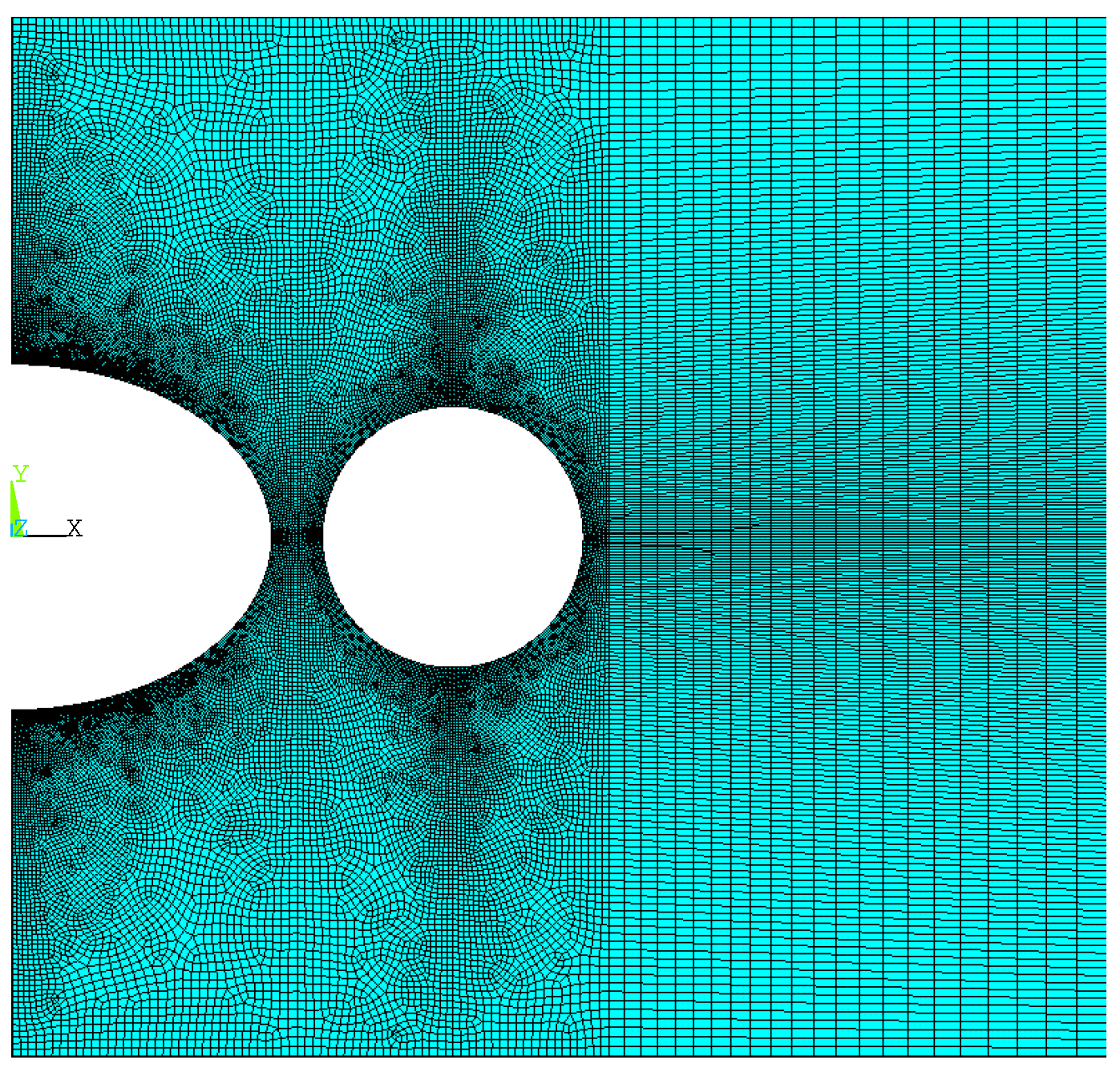
The mesh details of the finite element models used in the simple search method and parametric optimisation are shown in Figure 3 and Figure 4. These analyses were performed with the use of 2D PLANE182 elements with the plane stress assumption. The boundary conditions are shown in Figure 3. The criterion of the finite element mesh choice was the evaluation of the difference observed between the main stress σx and the estimated value of the searched solution (SMXB). As the limit, the difference between these two values was set to 2.0%. Such an approach is commonly acceptable from an engineering point of view.

2.2.2. Ansys Workbench Model

In the performed numerical analysis, the GDO applied in the Design Xplorer module of Ansys Workbench 2025 R1 [46] was used in the search for the optimal set of the listed parameters. The GDO is a set of constrained, multi-objective optimisation techniques in which the best possible designs are obtained from randomly generated sample sets with defined optimisation criteria, constraint conditions and an admissible range of the design variables set [47]. This technique is the development of a technique formerly used in Ansys, the Probabilistic Design Module. The numerical model of the analysed sample consisted of nearly 10,000 8-node plane elements. The boundary and load conditions were the same as in the parametric optimisation performed in Ansys APDL (Figure 3). In this analysis, for fixed elliptical hole dimensions, the optimal set of two parameters was sought, namely, the diameter of the relief hole (2r) and the distance between the elliptical hole and the relief hole (LW). Such analysis took into account the manufacturable values of the sought parameters. The design space included the hole diameter in the range from 5 to 30 mm with increments of 0.2 mm and the distance LW from 2 to 50 mm with increments of 0.1 mm. The goal of the optimisation was to minimise Ktn for the elliptical and the maximum value of the tension stress σx around the circular holes. Additionally, in the process, constraints limiting the maximum difference between Ktn for elliptical holes and the maximum value σx around stress relief holes to 10% were imposed. The Shifted Hammersley sampling algorithm (applied in the Ansys Design Xplorer module as a screening method) was used for sample generation. The Hammersley sampling algorithm is a quasi-random number generator, which has very low discrepancy and is used for quasi-Monte Carlo simulations. Application of such an algorithm provides a reliable estimation of the results with fewer runs when compared with Latin Hypercube Sampling, formerly accessible in the Probabilistic Design Module in Ansys.
In the studied case, the number of design points was set to 250, which appeared to be sufficient to obtain reliable results. This means that the algorithm generated 250 sets of design variables (2r and LW), and on that basis, the optimal solution was set.

2.3. Neural Network

An artificial neural network (ANN) was created with the use of the free and open-source TensorFlow [48] package. It is one of the most popular deep learning frameworks among others such as PyTorch [49]. TensorFlow is a software library for machine learning and artificial intelligence. This library can be used in a wide variety of programming languages, including Python, JavaScript, C++ and Java, facilitating its use in a range of applications in many sectors. The TensorFlow package was created by the Google Brain Team for internal use in research and production. The initial version was released under the Apache License 2.0 in 2015. In these studies, TensorFlow 2.19 with the Python language (PyCharm 2025.1.1.1 [50] and Spyder 6.0.5 with Python 3.12.9 64-bit [51], free Python-integrated developer environments) was used.
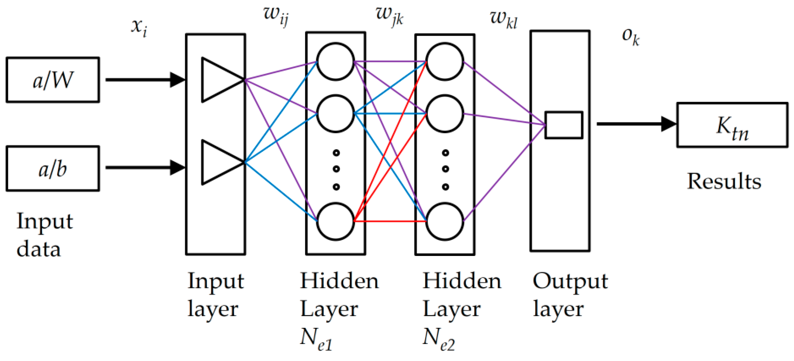
ANNs belong to computational models that mimic the construction of a biological neural network. Such models are composed of neurons in three groups of layers, namely, the input layer, one or more hidden layers and the output layer. The neurons in particular layers are connected and related to each other by weights. The weights are real numbers, whose values are determined during the learning process. An exemplary structure of the ANN is presented in Figure 5. The presented model is used to estimate the Ktn coefficients for specimens with elliptical openings. The input data (normalised values of the a/W and r/W ratios, where a is the length of the semi-axis of the ellipse perpendicular to tensile loading, r is the radius of the circular stress relief hole and W is the total width of the specimen—see Figure 1c) are introduced in the input layer and then processed in two hidden layers with Ne1 and Ne2 neurons. The output parameter (Ktn) (as one of several) is evaluated in the output layer.
To estimate the stress concentration factor and other parameters, three different networks for three cases, namely, (1) for a single circular hole, (2) for a single elliptical hole and, finally, (3) for an elliptical hole with two circular stress relief cut-outs, are created. The networks mentioned above differ from each other in the number of input and output neurons, as well as the number of neurons in the hidden layers. The input and output parameters for the particular cases are shown in Table 4. It should be noted here that in all cases, the input and output parameters are normalised with respect to their maximal values. The first two simple examples (with circular and elliptical openings, for which theoretical solutions exist) are investigated only to assess the impact of various network parameters on their accuracy. Based on these experiments, the ANN settings for the main third problem (elliptical hole with circular relief holes) are adopted.
In all studied cases, two hidden layers of neurons are used, whereby it is arbitrarily assumed that the number of neurons in the second hidden layer is equal to Ne2 = Ne1/2. The number of neurons depends on the studied case. All neurons have an additional bias. The number of neurons in the hidden layers is chosen as a result of the performed tests, which is discussed in the following section. In both hidden layers, the sigmoidal function is utilised as the activation function, whereas in the output layer, the activation function is linear.
In the first example (circular openings), the input parameter is defined as the ratio of circular hole diameter d and specimen width W. Based on this simple example, the influence of the number of hidden layers, number of neurons in hidden layers, number of epochs and size of training set on the accuracy of estimation of the output parameter (Ktn) is evaluated. In the second example (elliptical openings), the three ANN models are prepared with different numbers of neurons—{32,16}, {64,32} and {128,64}—and with a variable size of training set. The number of epochs is set to 350 iterations. The ratios a/b (semi-axes of the ellipse) and a/W are used as the input data. The main goal of these analyses is to evaluate the impact of the training set size on ANN accuracy.
In the last case of the elliptical hole with relief circular cut-outs, the number of neurons is set to {54,27}. Here, the following quantities are estimated: Ktn for the elliptical hole, the maximal stress around the circular hole, the equivalent of the Ktn coefficient for the circular hole, the maximal Ktn value for the elliptical hole with circular relief holes and, finally, Ktn for a single circular cut-out. It should be stressed here that for the assumed parameters (the size of the training set, number of epochs and architecture of the ANN), the training procedure should be repeated several times. At the beginning of the training process, the initial set of weights is randomly chosen. Therefore, each procedure of training starts from a different initial state and provides various results. In our studies, the training process is repeated from 3 (first case) to 5 times (last case).
For the supervised learning of a neural network, the Adaptive Moment Estimation algorithm is used with default learning parameters [48]. As a loss function and metrics, the mean square error (MSE) is assumed. However, for further analysis of the obtained results, other error definitions are utilised. The number of epochs (the number of complete iterations of the training dataset) of supervised learning, which ensures satisfactory results, should be greater than or equal to 350. No additional regularisation is applied to our ANN model.

Error Estimation

The accuracy of neural networks is controlled by means of commonly used loss functions (LFs). An LF function is a measure of how accurately a neural network fits the model to a given problem and training data. The LF is determined after neural network training (after the determination of neural network hyper-parameters), and it compares with the true (input) and predicted (output) values by the neural network. Therefore, taking into account the high accuracy of the neural network, the main aim is to minimise the LF value. In general [52], the LF can be divided into regression loss functions (such as mean squared error (MSE), mean absolute error (MAE), mean absolute percentage error (MAPE) and Huber loss) and classification loss functions (such as categorical cross-entropy and binary cross-entropy).
The first used LF measure is the MSE function, which is calculated as the average of the sum of k-elements of squared differences between the true y t r u e , i (input data) and predicted y p r e d , i (output data) elements:
M S E = 1 k i = 1 k y t r u e , i y p r e d , i 2
The MSE function is especially recommended for applications dealing with regression problems. The main disadvantage of MSE is that it is vulnerable to outliers due to the fact that the distance between true and predicted data is squared.
The second commonly used LF function is MAE, which provides the average value of the absolute differences between true and predicted elements:
M A E = 1 k i = 1 k y t r u e , i y p r e d , i
The models can also be controlled by the MAPE function, which calculates the percentage error between true and predicted values and is defined as follows:
M A P E = 100 % k i = 1 k y t r u e , i y p r e d , i y t r u e , i
This measure is mainly important in the case of problems in which variables change over a large range of values. In such a case, MAPE enables evaluation of the relative size of errors. A disadvantage of MAPE is that the true values cannot be equal to 0.
The adequacy of the ANN is assessed by means of the coefficient of determination (R2). The R2 quantity can be treated as the amount of variability in the data accounted by the regression model [53]. Such a statistical parameter is calculated by the following formula:
R 2 = 1 i = 1 k y t r u e , i y p r e d , i 2 i = 1 k y t r u e , i y p r e d , a v g 2 ,
It varies in the range from 0 to 1 ( y p r e d , a v g is the mean value of predicted values). Perfect prediction is indicated by R2 = 1; however, it should be noted that this parameter should be used with caution. It is reported that it is possible to increase the value of the R2 quantity by adding additional terms to the model, which, instead of improving the model, may worsen it and lead to an increase in MSE.
Additionally, the maximal difference between true and predicted values is controlled. Its value is calculated as follows:
M A X = max i y t r u e , i y p r e d , i
Summarising, the estimation of the artificial neural network approximation should include tracing more than one error estimator, which guarantees the proper setting of the process parameters.

3. Results of FEM Optimisation

3.1. Stress Concentration Around Circular and Elliptical Holes—Theoretical Study

The amount of stress concentration in the notch is specified by SCF (Ktn), which can be described as:
K t n = σ m a x σ n o m ,
where σ m a x is the maximal stress in the notch and σ n o m is the nominal stress, which is defined as stress in the weakened net cross-section. For example, in a tensile plate with circular or elliptical holes, the nominal stress is calculated by:
σ n o m = F t ( W 2 a ) .
Analytical formulas for determining the stress concentration factor for typical notches can be found in [3,4]. In the case of a rectangular plate of finite width with a central circular hole subjected to tensile loading, SCF is calculated with the formula given below:
K t n = 2 + 0.284 1 d W 0.6 1 d W 2 + 1.32 1 d W 3 ,
where d = 2r is the diameter of the hole and W is the width of the plate.
For a plate of finite width with a central elliptical hole that meets the condition 0.5 a / b 10.0 (a and b are the semi-axes of the ellipse according to Figure 1c), the solution SCF can be given as:
K t n = C 1 + C 2 2 a W + C 3 2 a W 2 + C 4 2 a W 3 ,
where
C 1 = 1.109 0.188 a b + 2.086 a b ; C 2 = 0.486 + 0.213 a b 2.588 a b C 3 = 3.816 5.510 a b + 4.638 a b ; C 4 = 2.438 + 5.485 a b 4.126 a b
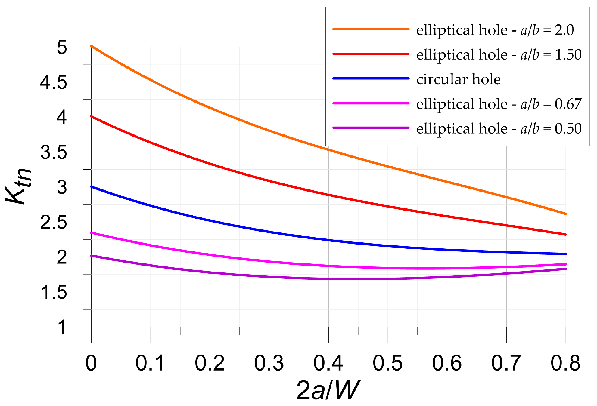
The comparison of the effect of circular and elliptical openings on SCF is shown in Figure 6.

3.2. Simple Search Optimisation Method

The value of SCF for the investigated specimen with a singular elliptical opening is equal to Ktn = 1.908 (theoretical solution—see Equations (10) and (11)) and Ktn = 1.922 (FEM calculations). The value of Ktn has an essential influence on the fatigue resistance and fatigue life. For this reason, it is crucial to minimise the value of SCF (Ktn). It is well-known that the stress concentration around a hole can be reduced by adding additional stress relief holes. Such holes must be located symmetrically with respect to the axis (perpendicular to the main load) of the main hole. This means that, taking into account the direction of the main stress, the holes should be located in front of and behind the main hole. Assuming that the relief hole will be a circular hole with radius r, the key problem is to determine its size and position relative to the main elliptical hole.
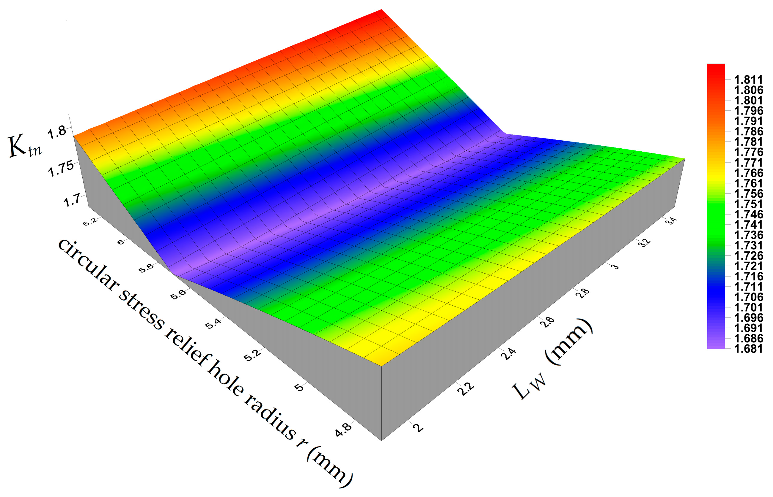
In order to illustrate this problem in detail, SSM is applied. The justification for using this method is that when a large number of points is used (with a high resolution), it allows for the most accurate representation of the shape of the objective function. This method is also effective for a small number of decision variables. Moreover, in the case in which the objective function depends on only two decision variables (as in the investigated case), it can be easily and clearly illustrated graphically in the form of a 3D surface. The main disadvantage of such an approach is that it is very time-consuming due to the large number of calculation points.
Here, the analysis is carried out for the following data: the semi-axis of the elliptical hole perpendicular to tensile load a = 7.5 mm and the second semi-axis of the elliptical hole b = 1.5a = 11.25 mm (Figure 1c). The remaining geometrical parameters are shown in Figure 1. Obviously, the radius r of the circular stress relief hole and the smallest thickness between the elliptical and circular hole LW are assumed as decision variables.
In further considerations, the variable LC, which determines the distance between the axes of circular and elliptical openings, will also be used instead of the variable LW. However, it should be noted that the variable LC is no longer fully independent (in contradiction to LW) because it also takes into account the influence of the radius r of the circular hole.
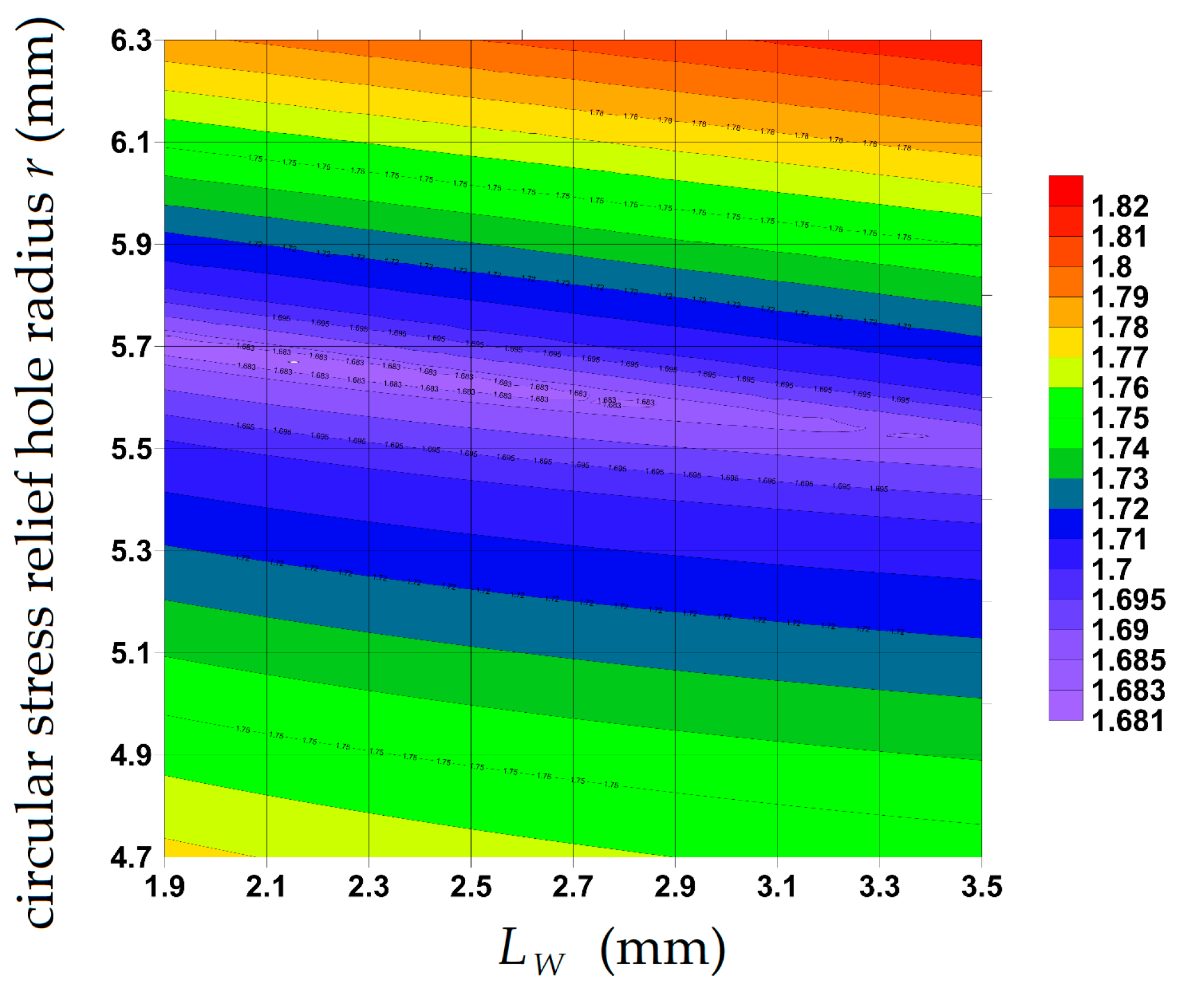
The results of this study for the following parameters
L W 1.9 ; 3.5 r 4.7 ; 6.3
are shown in Figure 7 and Figure 8.
In the plots, the presence of a relatively narrow and long area in the form of a strip with very low dependency between the design variables and the searched Ktn value is observed. Further conclusions may be taken up after observation of the topographic map shown in Figure 8. Here, a relatively weak dependency of Ktn is observed for LW, starting from 1.9 mm up to 3.3 mm and for r scattered around 5.6 mm to 5.7 mm values. This explains certain difficulties encountered in the exploration of the second path—APO.
It is obvious that there is only one optimal solution for which Ktn reaches the minimum value; however, there is a certain area of quasi-optimal solutions (purple colours in Figure 8) in which the Ktn values only slightly differ from the global minimum.
In order to obtain the smallest Ktn, circular relief holes should be made with fixed parameters r and LW. The radius r of the relief holes has a dominant influence in this case. The influence of the LW (or LC) distance is clearly smaller and has much less significance on the Ktn level (see Table 5). This is particularly important from a technological point of view related to the minimum wall thicknesses of the elements. It allows the minimum thickness LW between holes to be varied over a larger range without significantly increasing the Ktn value.
On the other hand, slight deviations from the optimal radius may result in a significant increase in Ktn. Depending on the technology used to make the holes (drilling, water cutting, laser cutting), there may also be manufacturing limitations. It is obvious that the greatest limitations will occur when using standardised drills. For this reason, for further analyses, it is assumed that the drill diameter must be rounded to 1 mm. Here, in the case of the use of a smaller radius for the relief hole than the optimal one, the negative influence of the smaller radius can be slightly compensated for by the increase in the distance between holes.
The global optimum with the minimum Ktn = 1.6806 is found for the following properties—r = 5.672 mm and LW = 2.163 mm (LC = 19.085 mm—point no. 3 in Table 5). Based on the results shown in Figure 7 and Figure 8 and the above explanation, the following hole parameters are adopted for the experimental research: r = 5.50 mm and LW = 3.25 mm (LC = 20.00 mm). The value of Ktn for such settings is only slightly larger than the optimal one (by 0.43%) and equal to 1.6879. However, this makes it possible to increase the wall thickness between the openings by as much as 62%. The remaining information, including the results for other settings, is provided in Table 5.

3.3. Parametric Optimisation Results

The numerical parametric optimisation performed in Ansys APDL 2024 R2 software can be carried out in two ways. The first one is the simplest and the fastest method, called subproblem optimisation (ZOOM). This is the zero-order method with a super-parabolic approximation of the objective function. In this solution, the optimal point is searched as a summit of the hyper-parabola in the search space, which is obtained on the basis of solutions in three neighbouring points. This method usually results in certain difficulties in the localisation of the global optimal point, where very small changes in the objective function are observed, and due to the truncation error, the solution can get stuck in a quasi-local optimum. To avoid this problem, the second approach with the more complex method of optimisation can be used, which belongs to the first-order optimisation method (FOOM). Such a procedure effectively uses the gradient value of the objective function to point out the direction of the next search. This method is time-consuming, but it reduces the risk of getting stuck in a local minimum. It is common practice in the numerical optimisation process that the application of both methods is admitted. It relies on making a series of optimisation loops with the application of the subproblem method, which usually results in a series of quasi-optimal solutions. The values of design variables corresponding to these quasi-optimal points are used as starting points in the next step of optimisation performed with the first-order method. Following that procedure, after several trials, the optimal solution of Ktn is found for the following values:
r = 5.6924   m m ; L W = 2.0013   m m .
In this case, Ktn = σx is equal to 1.6806.
It is worth mentioning that in the numerical analysis, changes in parameters usually influence the finite element mesh, changing the number of elements in the modelled domains. In order to eliminate or minimise this effect, the mesh should be constructed parametrically, taking into account the modification of areas near stress concentration zones with dense divisions to finite elements. Additionally, the quality of the mesh should be controlled by observing the SMXB parameter. In the performed analyses, the results are consistent to the third decimal place. The distribution of the σx stresses for the optimal configuration of parameters is shown in Figure 9.

3.4. Results of GDO Optimisation Process (Ansys Workbench)

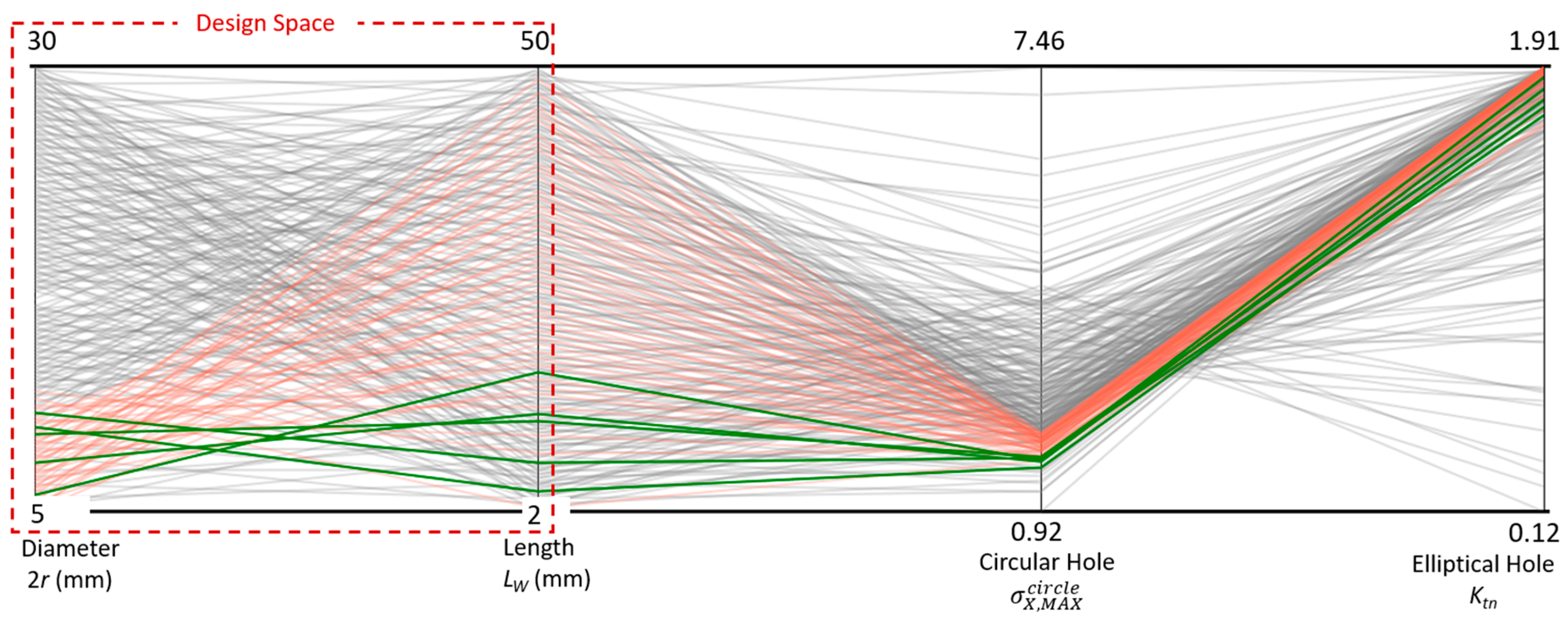
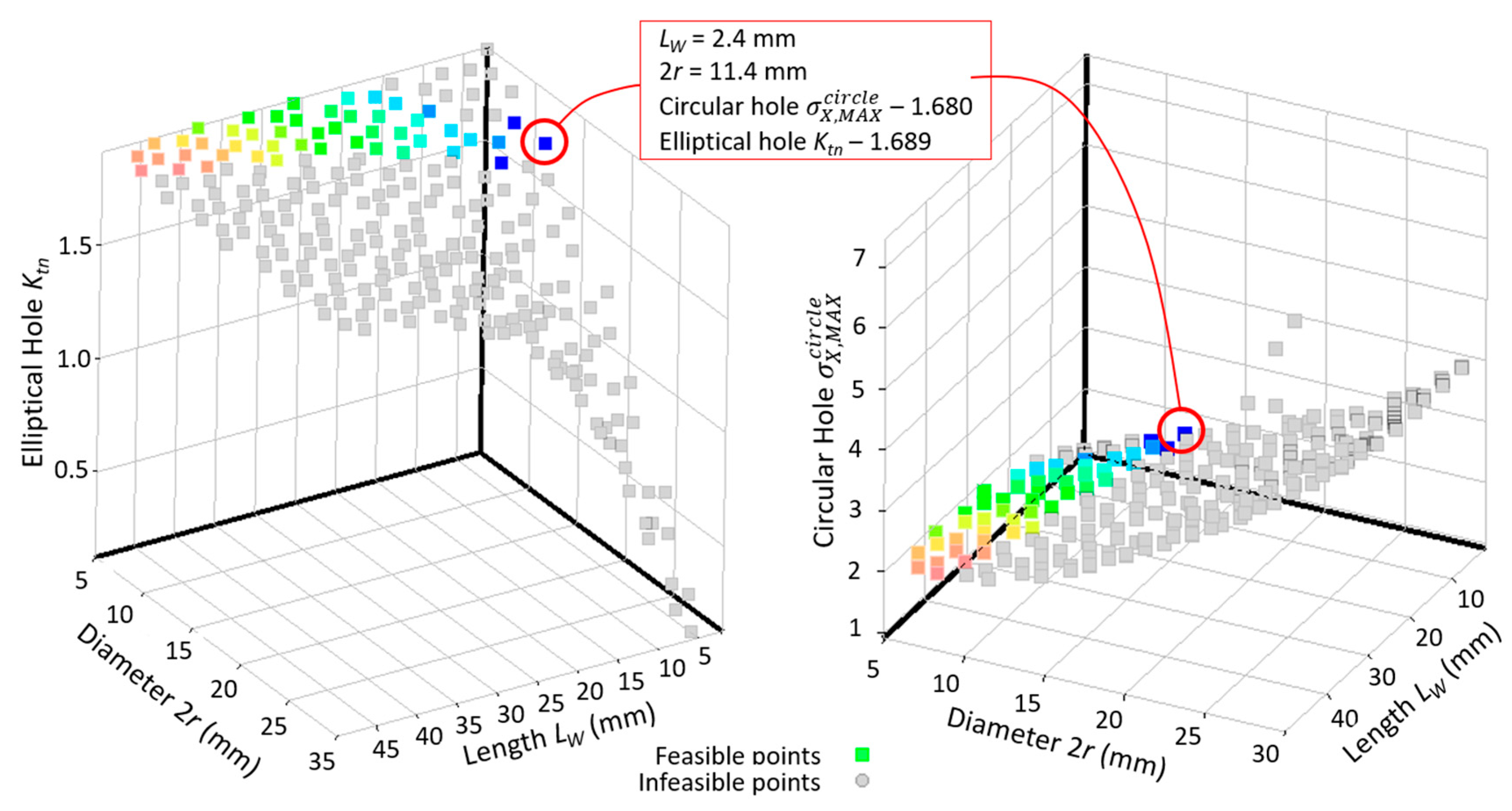
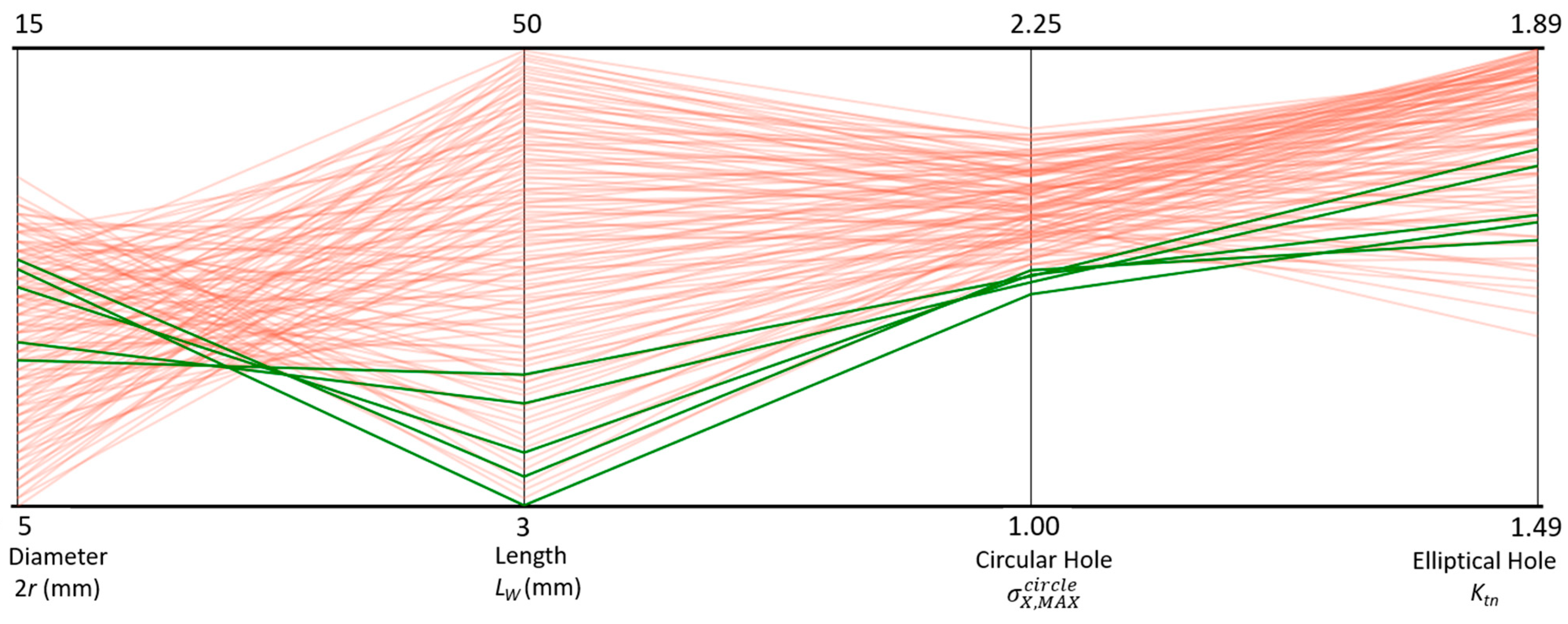
The Ktn value and the maximum σx stress are calculated for elliptical and circular stress relief holes, respectively, based on an analysis of 250 sets of design variables. The results of these calculations are presented in Figure 10. The figure shows the uniform population of the design variable space. The lines visible in the figure connect the set of variables (2r and LW) and the results obtained for this set.
Grey colour indicates a set of variables for which the maximum difference condition between Ktn values for individual holes has not been met. Orange indicates sets of design variables for which all optimisation conditions and constraints have been met. Green indicates sets of design variables for which the minimum stress concentration values have been achieved (Table 6).
The proposed optimal solutions meet all the search criteria. The minimum Ktn value for an elliptical hole is achieved at 1.689 (sample set 5 in Table 6), with a σ X , M A X c i r c l e value for a stress relief hole that is almost identical. The proposed solutions show that it is possible to achieve a lower value of the maximum stress σ X , M A X c i r c l e for a circular hole, but this comes at the cost of greater stress concentration at the elliptical hole. Figure 11 shows the relationship between decision variables and stress concentration factors for elliptical and circular holes, taking into account all calculated sets.
Assuming that reducing Ktn for an elliptical hole is the main factor in selecting the optimum allows us to present the influence of the desired length (LW) and diameter (2r) on the value of Ktn (Figure 12).
The results presented in the space of permissible solutions allow us to observe the characteristics of the influence of design variables on the stress concentration factor for an elliptical hole. However, it is worth emphasising that the optimal solution requires further analysis involving the local densification of design variable sets. Based on the results obtained, the optimal solution is verified by densifying the design variable space locally and increasing the minimum distance between holes slightly. The length (LW) varies from 3 to 30 mm in increments of 0.1 mm, and the diameter (2r) of the circular hole varies from 5 to 15 mm in increments of 0.2 mm. The other conditions of the analysis remained unchanged.
The results of the search for an optimal solution in the densified design space suggest that it is possible to achieve a lower stress concentration factor for a circular hole at the expense of a slightly higher Ktn value for an elliptical hole. Satisfactory solutions are obtained for different values of LW and 2r, which, given the relatively large difference between the calculated coefficients, indicates that there is no clear optimum (Table 7). On the other hand, if the criterion for selecting a solution is to minimise Ktn for an elliptical hole while keeping the difference between the coefficients as small as possible, the solution that meets the analysis conditions occurs for a similar value of the relief hole diameter and different values of LW (Table 8). The minimum Ktn value for the elliptical hole shown in Figure 13 is 1.638 for LW = 4.4 mm and 2r = 12.2 mm ( σ X , M A X c i r c l e for a circular hole in this case is 1.789, and the difference between the coefficients is 9.2%).
The relationship between the desired parameters and the Ktn value for an elliptical hole, taking into account all calculated sets of design variables, is shown in Figure 14.

4. Results of Neural Network Approach

4.1. Specimen with Single Circular Opening

It is obvious that there is a simple theoretical solution available on SCF (Ktn) for a circular opening (9), and the use of ANN for a single circular hole does not bring any practical benefits. However, for the case of a structure where the main opening (i.e., elliptical) is relieved by circular openings, such a theoretical solution no longer exists. Using ANN to evaluate such a problem with multiple openings offers substantial practical benefits. Therefore, ANN behaviour is also studied for a single opening to assess the impact of individual network settings and enable more effective network construction for the complex case with multiple openings.
The influence of the following settings of ANN on the evaluated Ktn value is investigated in this study: the number of hidden layers, the number of epochs, the number of neurons in hidden layers and the size of the training set. The ANN solver was trained based on data calculated from the theoretical formula (9) and validated by means of 51 points determined independently of the learning points. It corresponds to the case of the flat sample notched by a circular hole subjected to axial tensile loading. Both input and validation data are calculated for the ratio range d/W = 0.02–0.8, where d is the diameter of the circular opening and W is the width of the flat specimen. All data are normalised before being used in the ANN. Due to the fact that only one input data is required, the output parameter (Ktn) is described by a nonlinear curve.
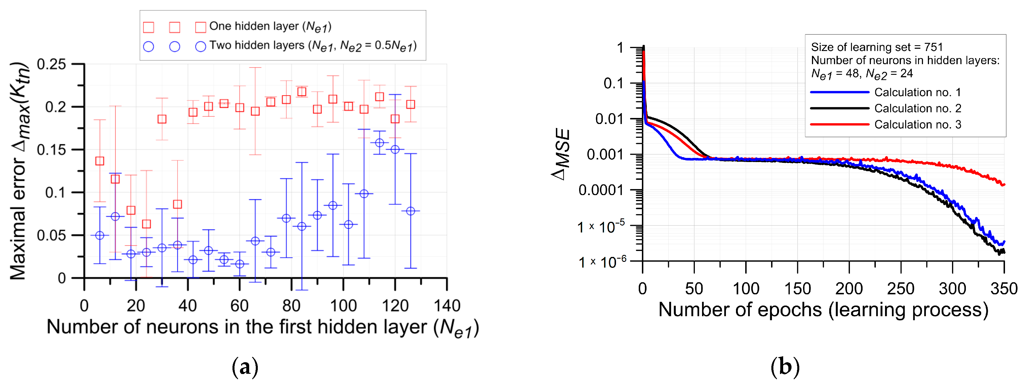
First of all, the influence of the number of hidden layers and the number of neurons in hidden layers on the maximal error is subjected to analysis. Calculations are carried out for a number of epochs equal to 350, a number of training elements 751 and a number of testing elements 51. For each point, three calculations are performed. The results of the ANN learning with a single and double hidden layer as a function of the number of neurons in the first layer are shown in Figure 15a. Here, the average values of the maximal error M A X and its standard deviation for each calculation point are presented in Figure 15a. It is worth noting that, according to the results of the initial tests, the single hidden layer of neurons is not enough to obtain satisfactory results in supervised learning. However, it can be seen that in the whole range, the maximal error is quite small. In the case of an ANN with two hidden layers, it was also een observed that there is a certain optimal number of neurons for which the maximal error and its dispersion are the smallest. Increasing the number of neurons above this level may result in decreased calculation accuracy.
The typical variation in the M S E during the ANN learning process is depicted in Figure 15b. This figure is prepared for a circular hole, where the size of the learning set is equal to 751, the number of epochs is equal to 350 and the number of neurons in the hidden layers are, respectively, {48 24}. As can be observed, at the very beginning of the learning process, the values of the M S E rapidly decrease. After that, the M S E value stabilises, and a further decrease in M S E is observed for epoch values above 150. Above 350 epoch count, the M S E generally reaches an acceptable level.
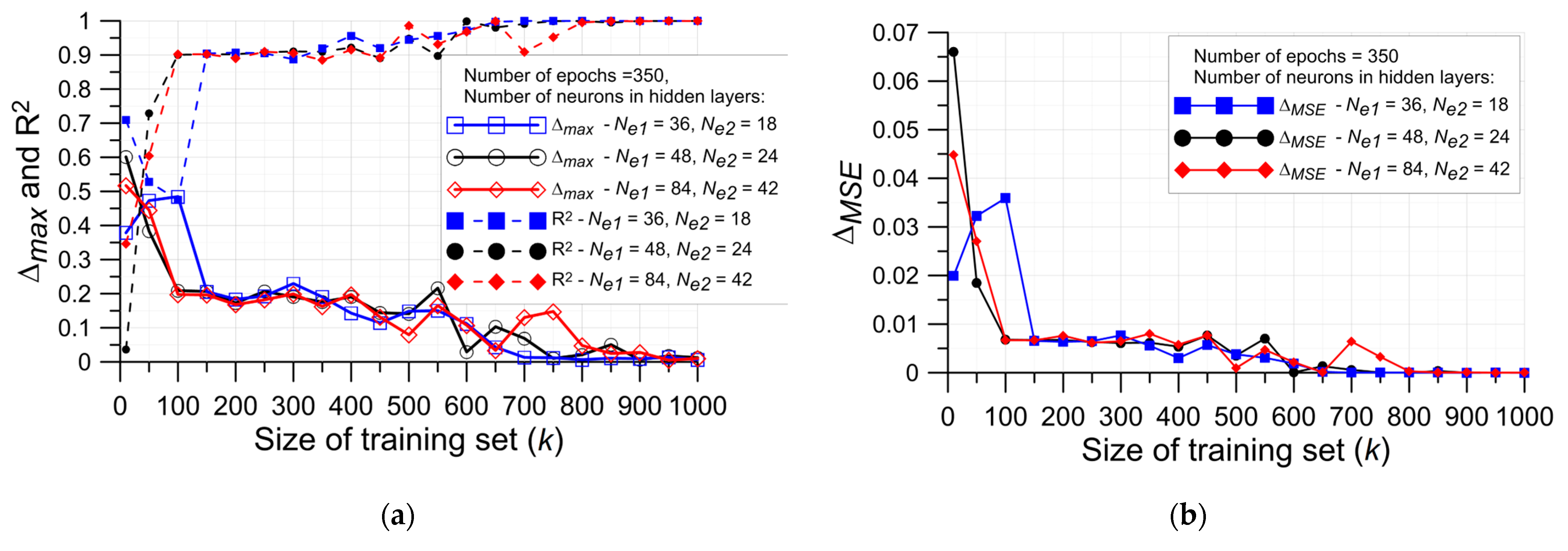
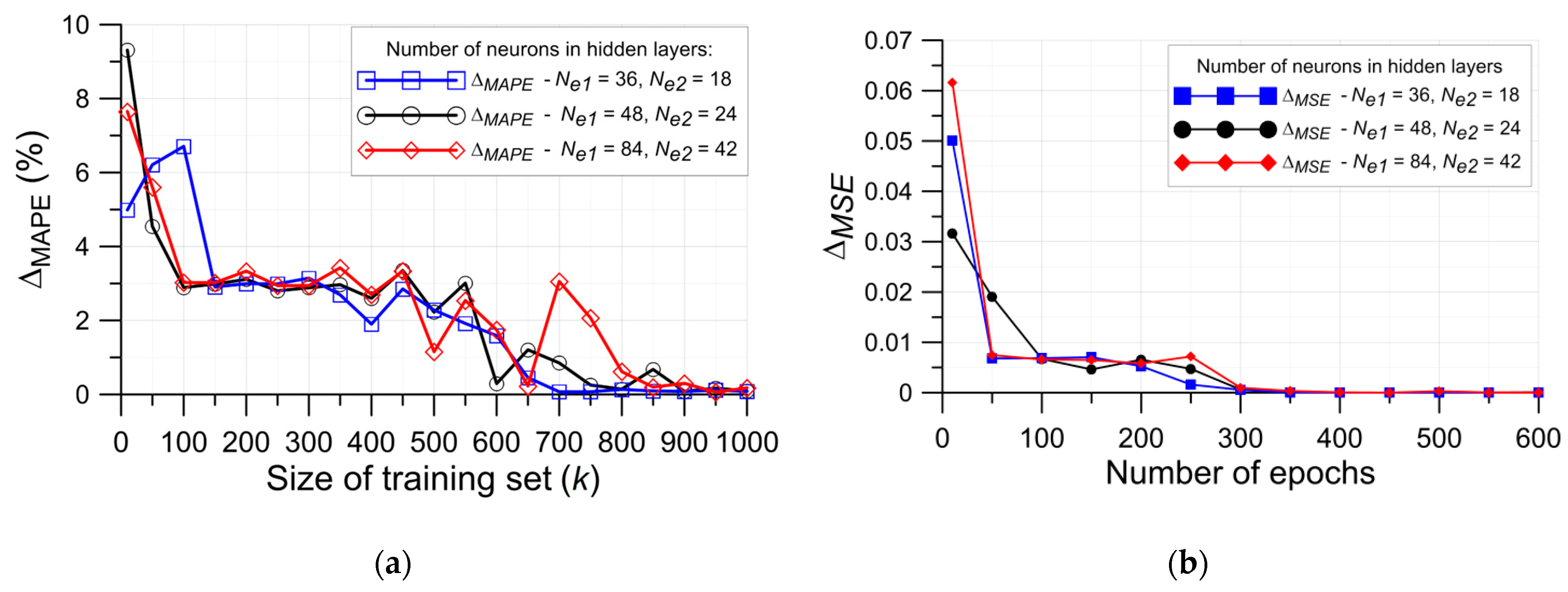
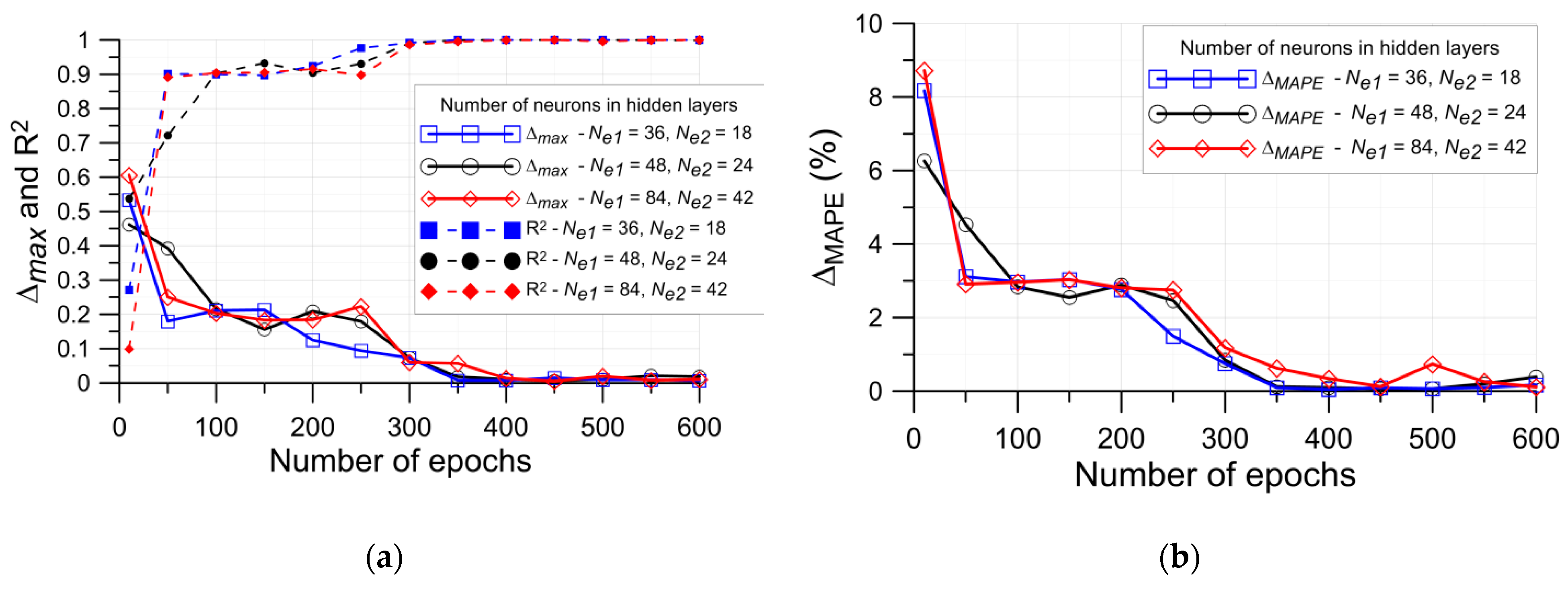
Based on the results shown in Figure 15, further calculations are made for ANN with two hidden layers with three different numbers of neurons—{Ne1 = 36, Ne2 = 18}, {Ne1 = 48, Ne2 = 24} and {Ne1 = 84, Ne2 = 42}. All results shown in Figure 16, Figure 17 and Figure 18 are performed on verification data. Three parameters are selected to assess the quality and accuracy of the network—three errors— M S E , M A P E and the maximal error and R2 parameter. The influence of the number of learning elements on a particular parameter is shown in Figure 16 and Figure 17a. The results obtained for networks trained with fewer than 100 training elements are not satisfactory (R2 < 0.9 and M A P E > 4%). Moreover, here, M A X is in the range 0.2–0.6, with the maximal possible value of Ktn = 3, which results in a relative error in terms of 7–20%. In the case of networks with a smaller number of neurons (Ne1 = 36 and 48), a significant reduction in error values ( M A X < 0.1) and an increase in the R2 parameter (>0.99) occurred when more than 600 training points were used. The network with the largest number of neurons (Ne1 = 84) achieved stability when more than 750 points were used.
When comparing individual results in Figure 16b with Figure 16a and Figure 17a, it can be seen that M S E has the same trend as the remaining errors, but its value does not allow for a full assessment of the accuracy of determining Ktn by ANN.
A similar trend is observed when the number of epochs is set as a variable. Here, acceptable accuracy (R2 > 0.99, M A X < 0.1, M A P E < 1%) is obtained in all cases for a number of epochs larger than 300.

4.2. Specimen with Single Elliptical Opening

A similar analysis is performed for the case of an elliptical opening. The input data are obtained using the dependencies (10–11). In contrast to the previous case with a circular opening, here, two input parameters are required. The first one (a/b) defines the ratio of the semi-axes of the ellipse and is used in the range of 0.5–2.0. The second one (a/W) describes the size of the horizontal semi-axis a of the ellipse in relation to the width W of the sample within the range of 0.02–0.4. The value of the SCF is calculated for the case of the axial tensile loading, in which the tensile force is perpendicular to the semi-axis a. Therefore, the problem of a specimen with an elliptical hole is more complex than that with a circular opening. Due to the two input parameters, the solution of Ktn has the form of a nonlinear surface. The input data is prepared in the form of an array ke × ke with the same number of points (ke) for both input variables. Therefore, the total number of input data points i is equal to k e 2 .
The network settings are set based on the conclusions observed and presented during ANN analyses of the circular opening (Section 4.1). Three different numbers of neurons in hidden layers are assumed—{Ne1 = 128, Ne2 = 64}, {Ne1 = 64, Ne2 = 32} and {Ne1 = 32, Ne2 = 16}. In each case, calculations are carried out with epochs number equal to 350. The main objective of this study is to evaluate the accuracy depending on the number of input data i.
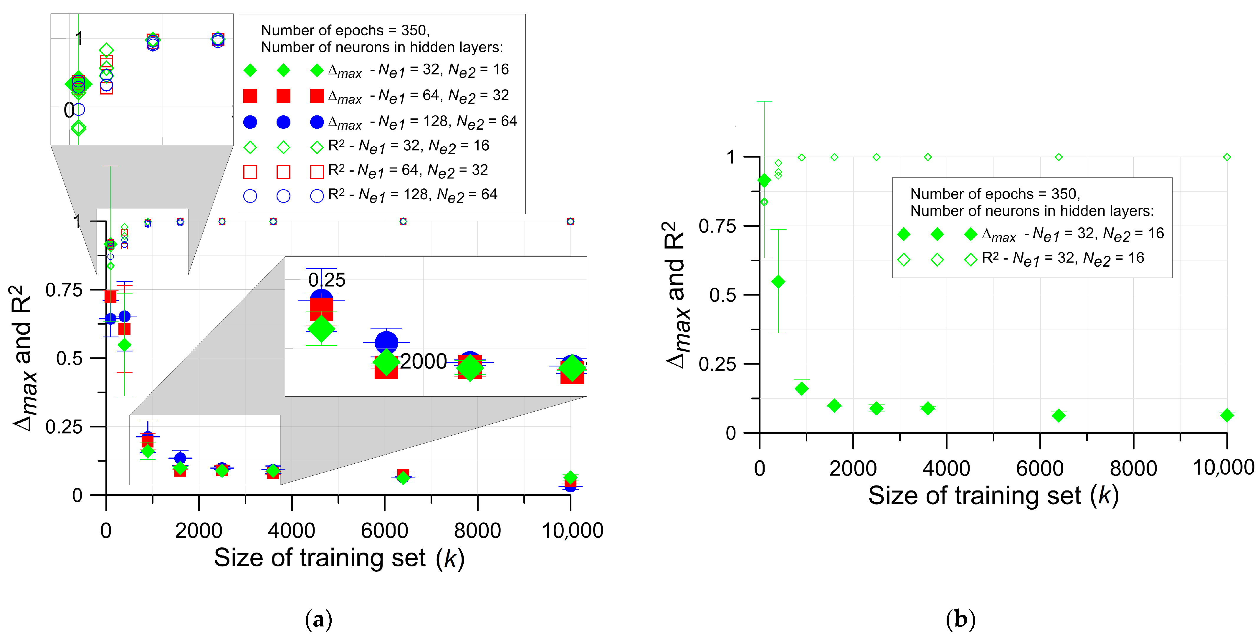
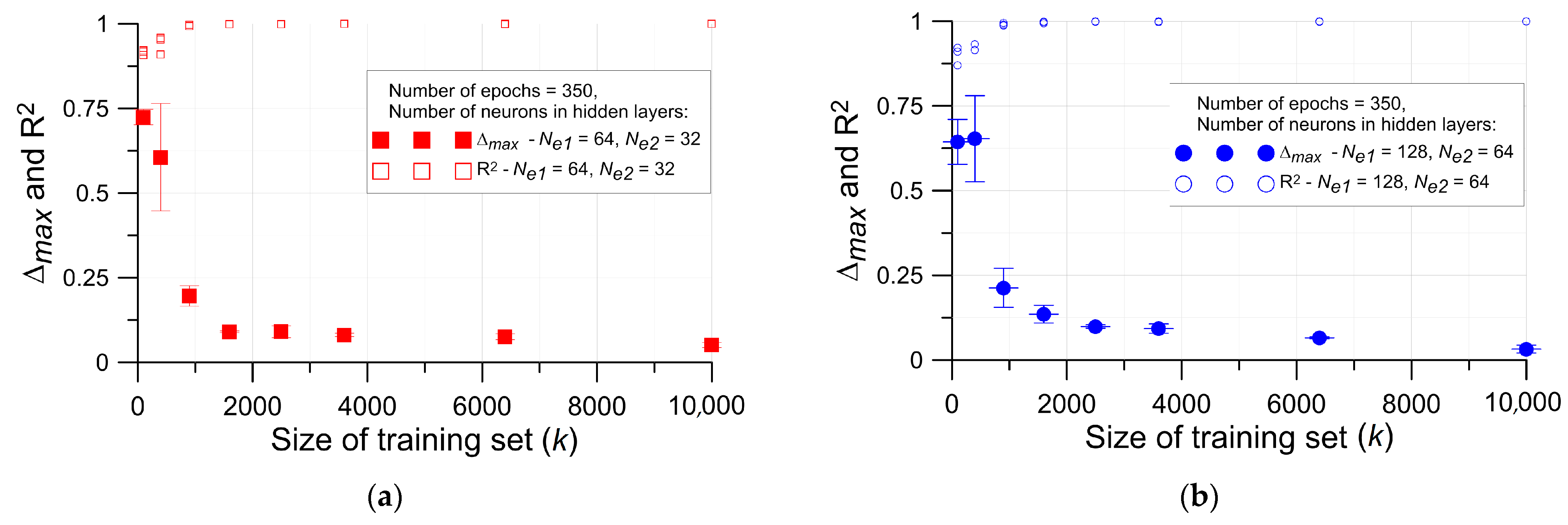
The results of the study are presented in Figure 19 and Figure 20, in which the maximal difference between the true and predicted M A X and R2 parameter is presented. The maximal value of Ktn in the investigated area is equal to 4.809. It should be noted that the error M A X describes a difference between the original and predicted data at the point at which the highest discrepancy of Ktn between the original and predicted data occurred. Such an error can occur locally in a small area, usually at the boundaries of the decision variables.
The network’s accuracy across the entire investigated area is represented by the R2 parameter. The network with the smallest number of neurons {Ne1 = 32, Ne2 = 16} leads to the highest errors (even M A X = 1.09 , which is a relative error equal to 23%) with a large spread for a small number of training data (when k < 500). Increasing the number of neurons slightly reduces the error M A X and scatter of the results.
Assuming the error M A X 0.1 as the network evaluation criterion, the following minimal size of training set was necessary:
  • for (Ne1 = 128, Ne2 = 64)—k ≥ 2500,
  • for (Ne1 = 64, Ne2 = 32)—k ≥ 1600,
  • for (Ne1 = 32, Ne2 = 16)—k ≥ 1600.
For the above number of input data, the predicted results had high accuracy for the range 1.5 < a/b < 0.67. Convergence is most difficult to achieve for the range a/b ≤ 0.67. The highest errors occurred in the corner (a/b = 0.5 and a/W = 0.4). Acceptable high accuracy (only with slight discrepancies at the boundaries) in the entire assumed area was obtained when the training set had at least 6400 points. Essentially, full agreement ( M A X   < 0.03 ) was observed when the training set had at least 40,000 points.
The aggregate error over the entire investigated area is evaluated by M A P E error and is presented in Figure 21. In this case, a larger number of neurons {128,64} reduced the maximal error M A X (see Figure 19a); however, it increased the aggregate error. This means that there was an increase in estimation inaccuracy over a larger range of decision variables. On the other hand, too small a number of neurons led to a larger error M A P E for a small size of the training set. However, for a large set of training data, the differences were negligible.

4.3. Determination of Optimal Configuration of Stress Relief Holes and Maximal Ktn Value

The investigated problem (Figure 1b) has no theoretical solution, and due to the complexity of the objective function shape, it is difficult to study. In the case when the impact of the relief holes on the stress concentration factor Ktn is studied, two variants of the application of the ANN are analysed. In the first case, the training set and the testing set of data are randomly generated from a relatively wide range of values of the decision parameters (1 ≤ r ≤ 20, 12.25 + rLC ≤ 64.25; in mm). The optimal structure of the ANN is sought, namely, the number of neurons in the two hidden layers. Next, the optimal configuration of the relief holes is estimated with the highest possible accuracy for the narrowed range of input parameters. Utilising the results obtained from the analysis of the single circular hole and the single elliptical hole (Section 4.1 and Section 4.2) in both variants, the total number of epochs in the training process is set to be equal to 850. Moreover, the sizes of the training sets are equal to, respectively, 8750 and 8550 for the first and second variants. In both cases, the size of the testing sets is equal to 50.

4.3.1. Sub–Variant 1: Extended Feasible Range of the Input Parameters

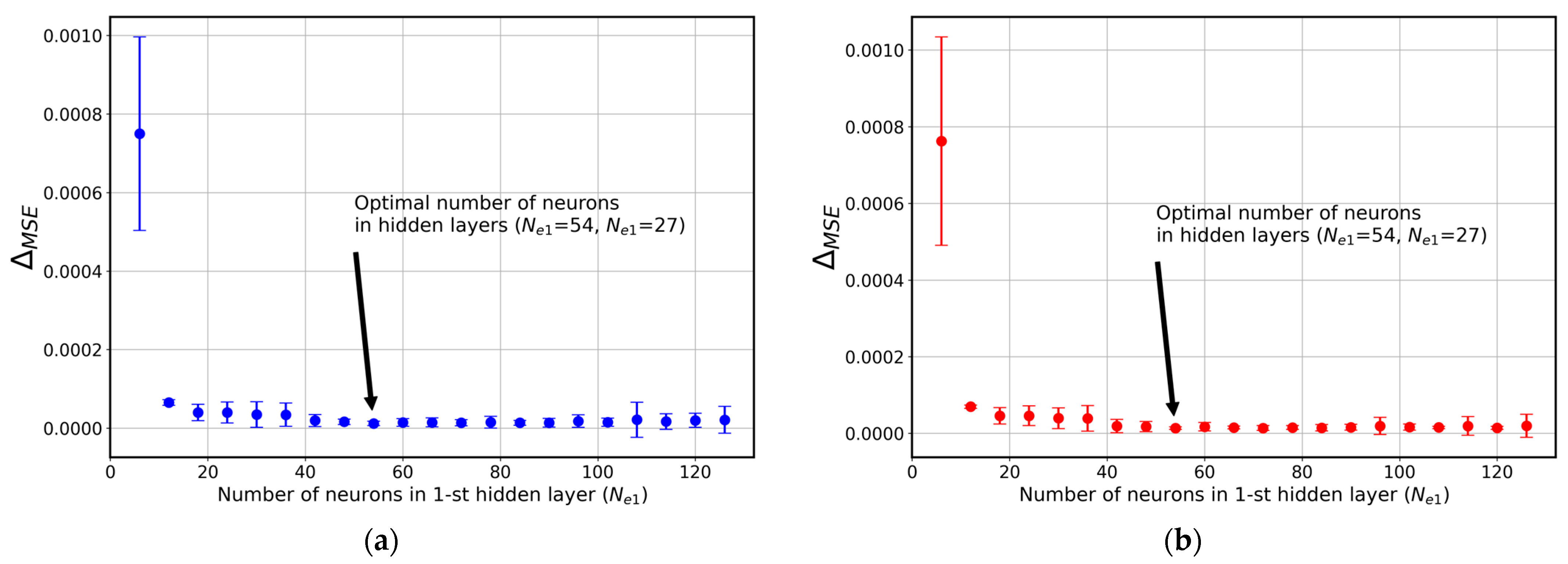
In this variant, the input parameters, namely, the radius of the relief circular hole and the distance between the axis of the elliptical hole and the axis of the circular hole, are randomly generated from the ranges 1.014 mm–19.996 mm and 13.746 mm–64.230 mm, respectively. The sets of points uniformly cover the feasible range of parameters. Firstly, the optimal number of neurons in the hidden layers is determined. The computations are performed for the following pair of neuron numbers: {6, 3}, {12, 6}, {18, 9}, …, {126, 63}. For each pair, the training procedure is repeated five times. The M S E error as a function of the number of neurons in the first hidden layer is shown in Figure 22a,b. In the first graph, the M S E error is taken from the last epoch of training, while in the second graph, the M S E error is computed based on the testing set. As can be observed, together with increasing the total number of neurons, the value of the mean as well as the value dispersion of the M S E error decreases. Based on the presented results, the following number of neurons is assumed for further analysis: 54 neurons in the first hidden layer and 27 in the second hidden layer.
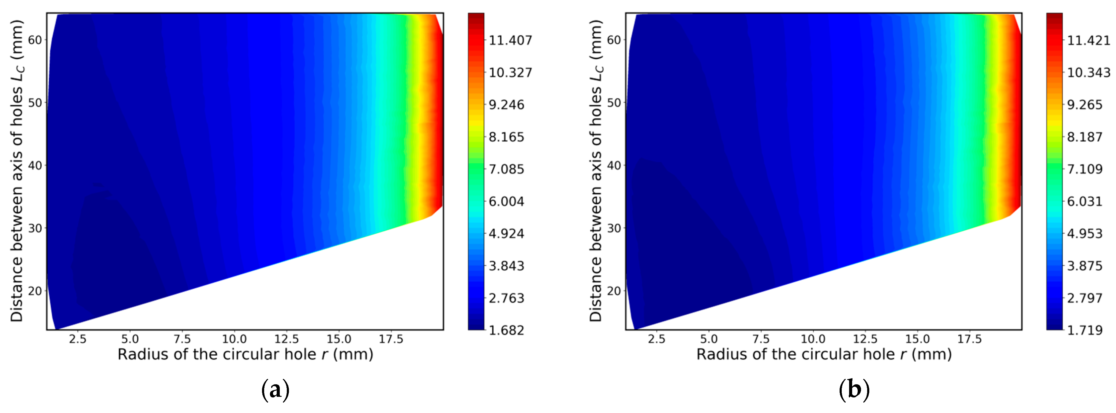
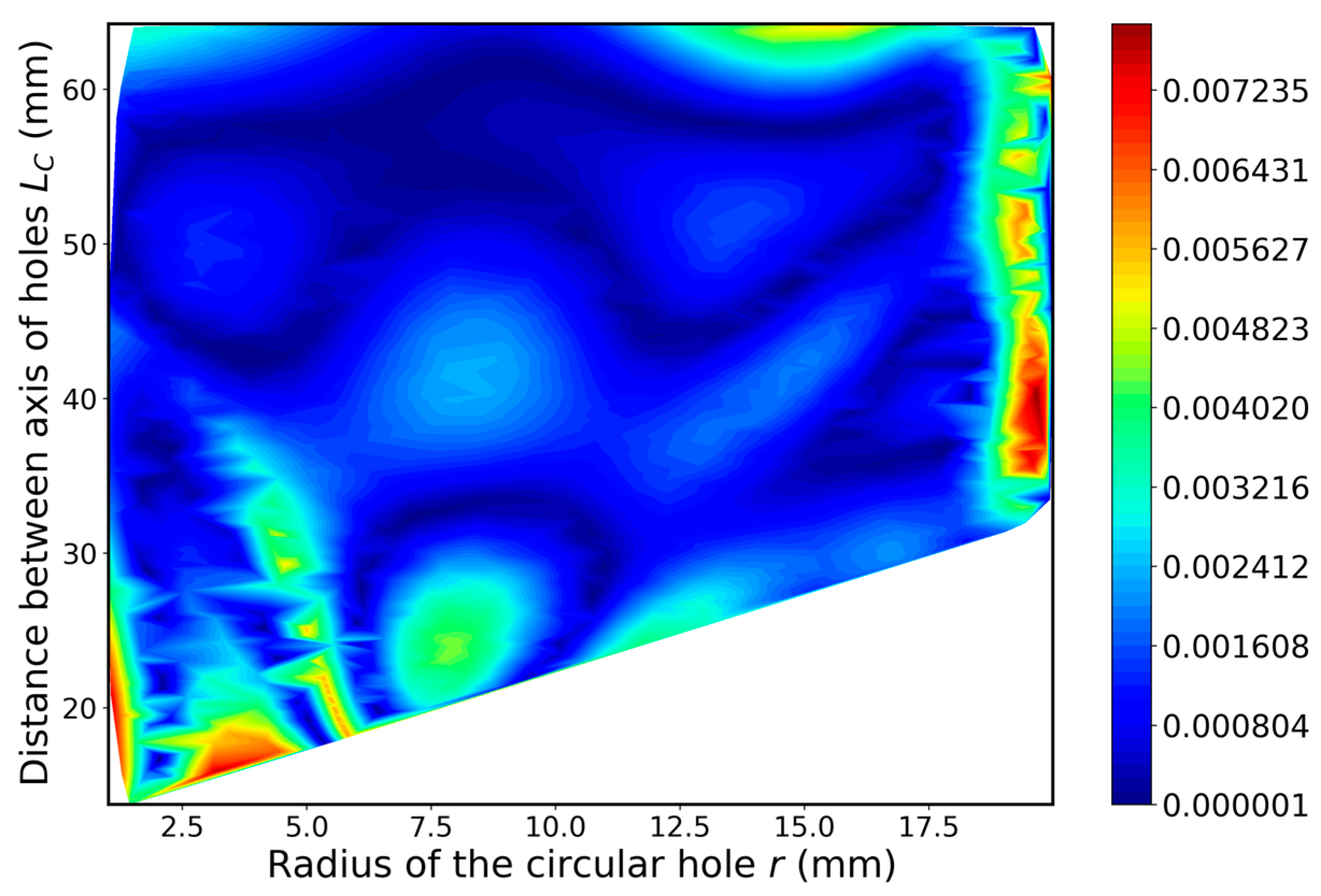
Next, the value of the Ktn coefficient as a function of the input parameters (radius of the stress relief circular hole and the distance between axes of the elliptical and circular cut-outs) is shown in Figure 23a,b. The left graph is generated from the training set (numerical solution), while the right one is obtained from the trained ANN. In both cases, the global minimum is in the lower left-hand corner of the graphs. The relative error in each point, defined as |ytrue,iypredict,i|/ytrue, max, where ytrue, max = 12.308 mm, is shown in Figure 24. As can be observed, the relative error is not uniformly distributed over the feasible range of input parameters. However, its maximal value does not exceed 1%. Similar results are obtained for the rest of the output parameters (not presented here).
The optimal input parameters, obtained from numerical analysis and a trained ANN, are depicted in Table 9. The solution, estimated from the trained ANN in comparison with the numerical one, is not satisfactory. Therefore, it was decided to update the feasible range of the input parameters and narrow them in the surroundings of the global minimum.

4.3.2. Sub-Variant 2: Narrowed Feasible Range of the Input Parameters

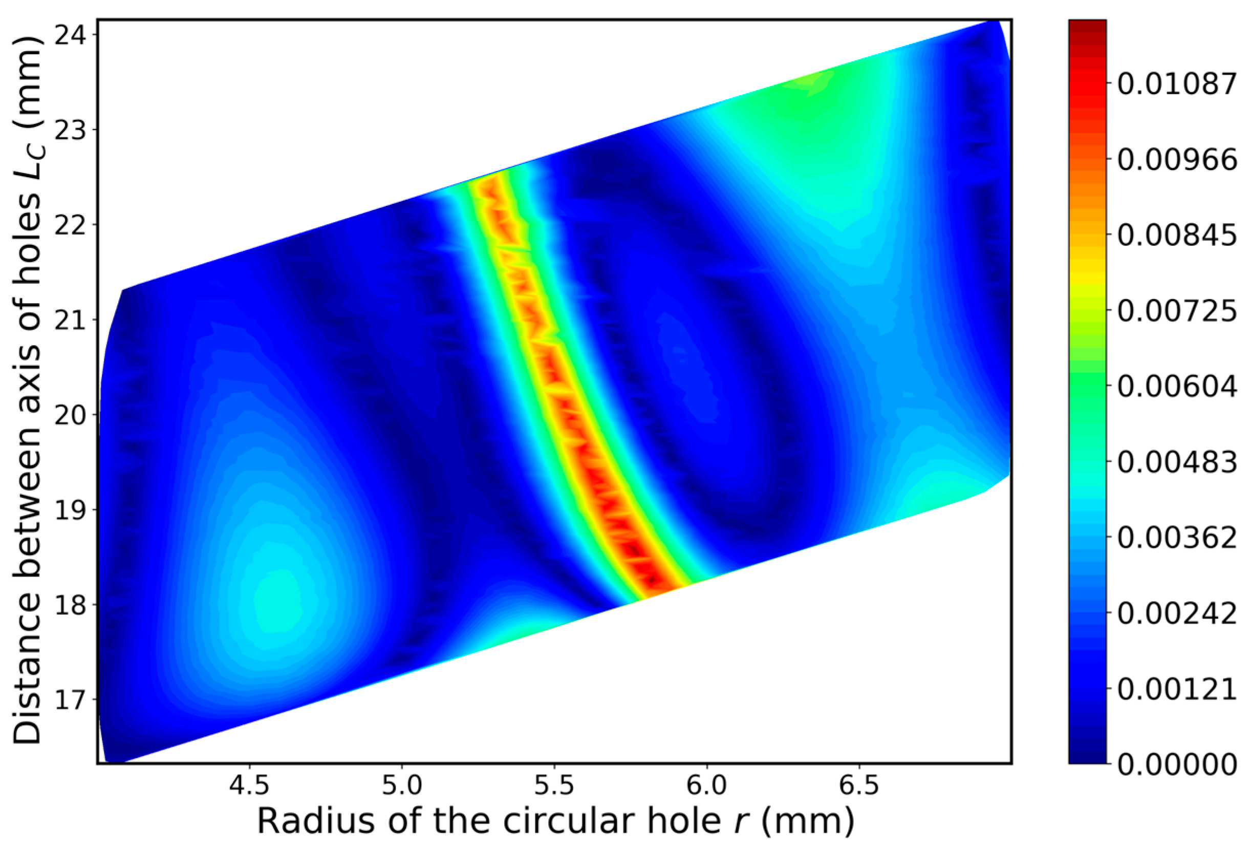
Now, the feasible range of the input parameters is as follows: the radius of the relief hole r varies from 4 mm to 7 mm, and the distance between the axis of the ellipse and the axis of the circular hole LC varies from 16.323 mm to 24.152 mm. As before in the case of sub-variant 1, the sets of points uniformly cover the updated feasible range of parameters. The number of neurons in the hidden layers is identical to that assumed in sub-variant 1.
The value of the Ktn coefficient as a function of the input parameters is shown in Figure 25a,b. It should be noted that the accuracy of the new updated solution is significantly better in comparison with that presented for sub-variant 1. However, the maximal value of the relative error, where ytrue,max = 1.966, is a little bit higher than in sub-variant 1 (Figure 26).
The values of the optimal input parameters for sub-variant 2 are collected in Table 9. It should be stressed now that, in our opinion, the updated solution is quite satisfactory.

5. Experimental Results of Fatigue Tests and FEM Analyses of Notched Specimens Reinforced by Composite Overlays

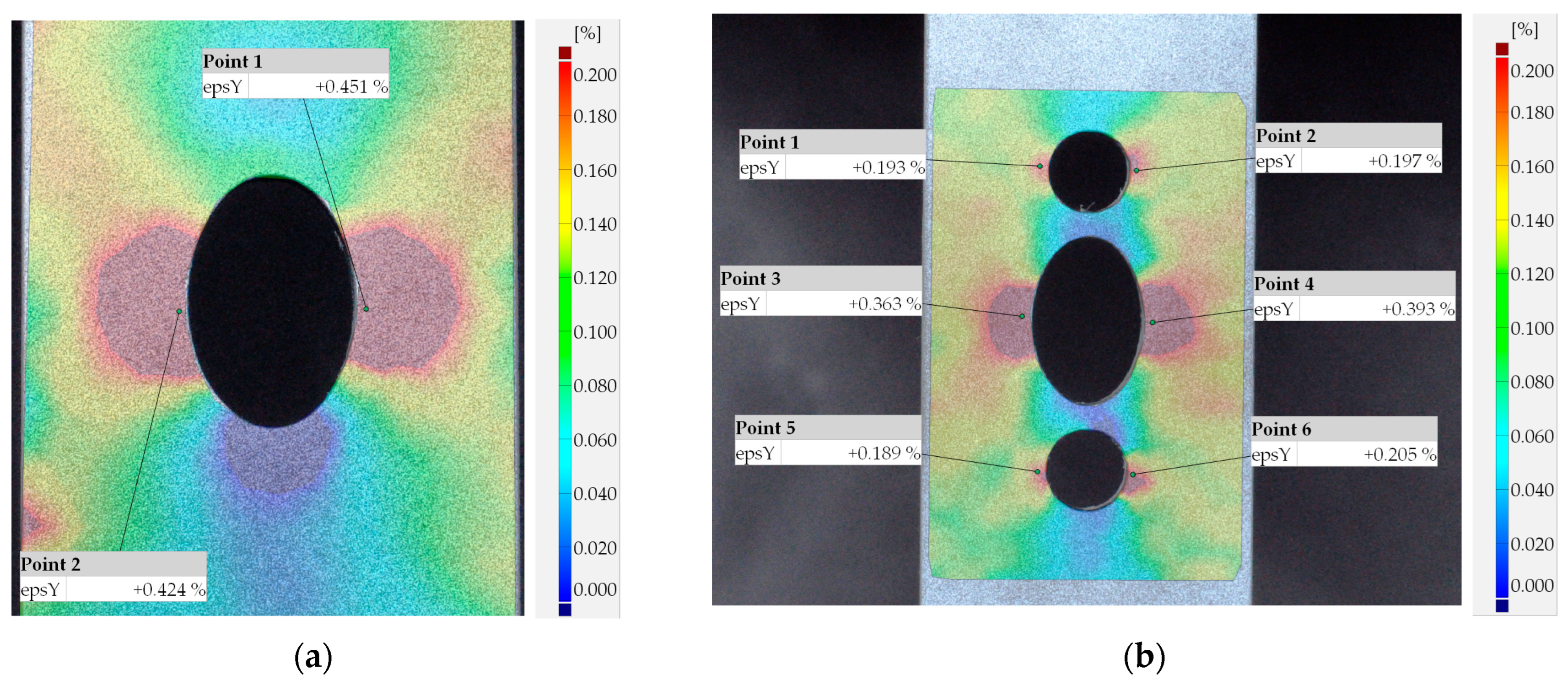
The results of the experimental fatigue tests are obtained for specimens with a singular elliptical hole and for samples with an elliptical hole with two circular stress relief holes. The fatigue failure modes are shown in Figure 27. The effect of the application of circular stress relief holes is presented in Figure 28, in which the comparison of principal strains for a singular elliptical hole and an elliptical hole with circular stress relief holes is presented. These results are obtained from digital image correlation analyses performed in the GOM Correlation Software 2018 [54]. In both cases, the images are made for a static tensile force equal to 40 kN. A detailed description of the measurement system is given in reference [55]. It can be seen that the application of stress relief holes significantly reduces the maximal strains around the main elliptical hole and areas in which high strains occur. The contour map for the specimen with stress relief holes can be compared in a qualitative sense with the FEM solution presented in Figure 9 (FEM analysis is carried out for a force equal to 120 N). The remaining data from the experimental studies are given in Table 10. The values of Ktn are calculated with the use of FEM. Additionally, FEM analyses are carried out for both above samples reinforced by composite overlays with thicknesses equal to 2 mm (the remaining details are shown in Figure 1d). The glass/epoxy composite has the following mechanical properties: E1 = E2 = 25.3 GPa, ν12 = 0.28, ν21 = 0.4, G12 = 7.9 GPa. Such FEM analyses are carried out for different stiffnesses of the adhesives. The values of stiffness are selected on the basis of previous studies by the authors [13]. The application of composite reinforcements is justified in previous studies by the authors [13,15,56]. Based on the experiments and data reported in the literature [14], it is observed that, depending on the adhesive used, the fatigue life increase may vary from 20–890%. The exemplary FEM results for specimens with elliptical holes reinforced by composite overlays are shown in Figure 29.
The fatigue lives of each tested specimen (including the average fatigue life and standard deviation) with a singular elliptical hole as well as with an elliptical hole with two circular relief holes are given in Table 10. Here, also, the values of Ktn calculated by FEM simulation for all investigated examples are reported. It can be seen from the experimental tests that there is a clear dependence between Ktn and fatigue life.
Based on the obtained FEM results for samples reinforced by means of composite overlays, in which Ktn is additionally reduced in comparison with bare steel samples, it can be concluded that the application of the composite overlays provides further opportunity for increasing fatigue life. The highest reduction in the Ktn value is obtained when two circular relief holes and four composite overlays are applied.

6. Discussion

The results of the optimisation studies are presented in Table 11. Here, two kinds of solutions are reported. In the first case (global), the optimal Ktn value is evaluated based on calculations over the entire range of variability of decision variables (r, LW). In the second case (local), an additional constraint condition (LW ≥ 3 mm) has been added on the variable defining the minimum wall thickness between holes. SSM, which is the most time-consuming procedure, allows for the determination of the points at which the lowest values of Ktn occurred. Here, two points in which Ktn obtained similar values (1.6806; differences are within the range of FEM solution accuracy) are reported. The main difference between these two points is the LW distance. The global optimal points found by means of APO are close to the optimal point found by SSM. However, such calculations are also time-consuming. The optimal global solution indicated by GDO differs little from the SSM and APO solutions. This is caused by a larger range (5 mm ≤ 2r ≤ 30 mm and 2 mm ≤ LW ≤ 50 mm) and higher increment (0.1 mm in order to reduce the time of analyses, which is about 10 h) of the considered decision variables than in the cases of the previous analyses. Because of this, the GDO solution can be regarded here as an initial one, and in the vicinity of the indicated point, the additional local calculations with the finest increment of decision variables should be made. In the case of ANN, macro calculations in which the input data had a large range (1 ≤ r ≤ 20, 12.25 + rLC ≤ 64.25; in mm, for which Ktn is in the range of 1.68 ≤ Ktn ≤ 12), the relative error of the determination of the optimal points is as follows:
  • Error of radius r determination: r = –15.6%;
  • Error of stress relief hole position LC:   L C = –9.5%.
This is caused by the fact that the area in which the optimum occurs is a narrow strip and that Ktn in the introduced input data changes by an order of magnitude (Figure 23). The limitation of the range of the decision variables (ANN—local method) allows for the determination of the optimal point with sufficient accuracy ( r = 1.7 % ,   L C = 1.3%). In both cases, in the application of ANN, the results are obtained in a short time. However, the largest difficulty in this case is the preparation of the input data. It becomes important if high accuracy of ANN is required, where a large training set is necessary. The determination of such a large amount of input data is generally time-consuming. On the other hand, ANN’s advantage is as follows—it only needs one training procedure, and after that, a different set of solutions can be obtained in a relatively short time.
A similar trend is obtained for the local scale, in which an additional limitation (LW ≥ 3.0 mm) is included. Based on such local-scale analyses, the geometry of the relief holes is assumed (r = 5.5 mm and LW = 3.25 mm).
The performed experimental tests and FEM analyses confirmed the validity of optimisation focused on the minimisation of stress concentration around openings. Cutting out two circular stress relief holes not only reduced the sample mass but also increased the fatigue life by about 79%. This is caused by a reduction in Ktn by about 12%. It is also shown that application of additional reinforcement in the form of composite overlays may additionally reduce Ktn by about 7% (in the case without stress relief holes) and 17% (in the case with two circular stress relief holes) with respect to a bare specimen with an elliptical hole and without stress relief holes cut. The comparison between a specimen with stress relief holes (Ktn = 1.688) and with a specimen with the same stress relief holes but also reinforced by composite overlays (average Ktn = 1.592) justifies the application of composite reinforcement in order to increase the fatigue life (Ktn is reduced by about 6%).
It should also be noted that in the investigated case, in which only two decision variables are considered, the possibilities of ANN have not been fully exploited. The introduction of additional decision variables (i.e., different geometries of the main opening, various ratios of ellipse semi-axes, variable size of main hole and specimen width, larger number of stress relief holes, etc.) should increase the benefits of ANN’s application compared to the remaining optimisation methods.
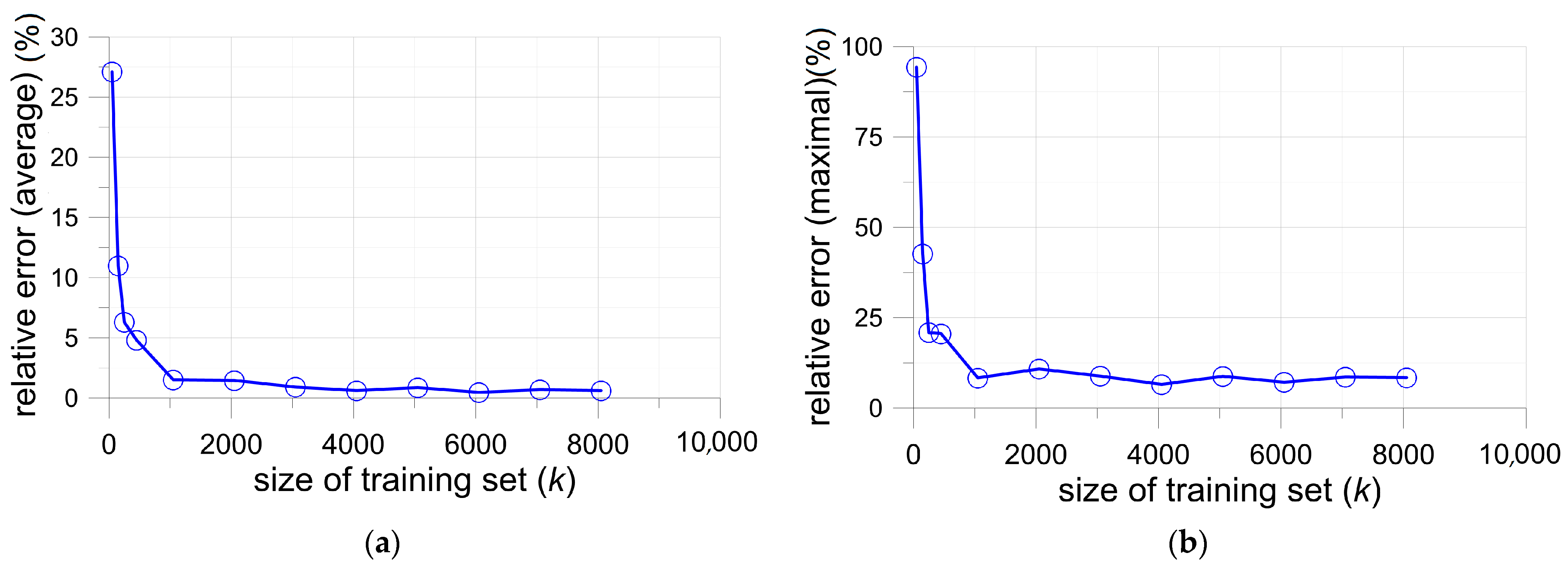
In order to evaluate the capabilities of neural networks in the determination of the Ktn value, additional calculations with limited input data are performed. The size of the training set is varied from 50 to 8000 input data. The input data is generated by FEM for random radii (within a range of 1.0 mm ≤ r ≤ 20.0 mm) and positions (within a range of 13.7 mm ≤ LC ≤ 64 mm) of circular stress relief holes. The average and maximal relative errors of Ktn determination are shown in Figure 30a and Figure 30b, respectively. It is observed (Figure 30a) that the average error dropped below 7% even with a small size of input data (k ≥ 250). However, with such a small number of input data, some errors occurred at the boundaries of the investigated area, which led to an increase in the maximum errors (Figure 30b). For the size of the training set k > 1000, the average relative error is below 2%.
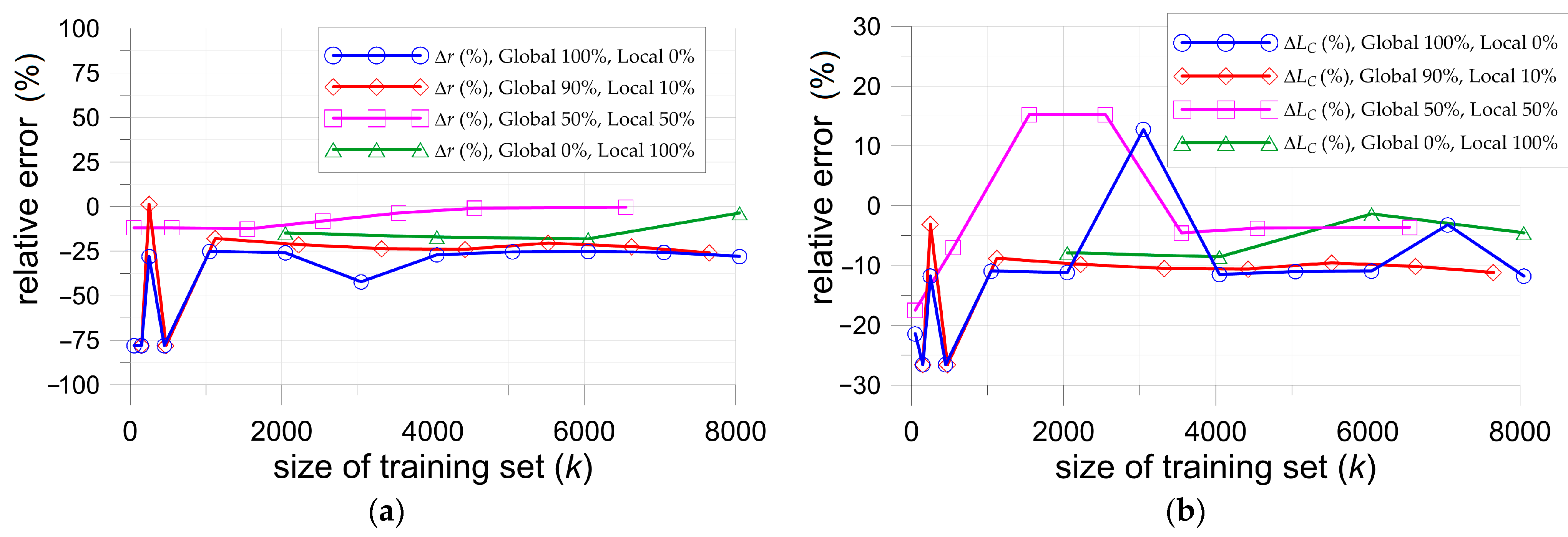
The relative errors in determining the optimal geometry of circular stress relief holes (radius r and distance LC) using ANN for different sizes of the training sets are shown in Figure 31. The results are related to the global optimum (determined by SSM) posted in Table 11. The calculations are made for four different datasets with different ratios for the global and local range. In the case of the global range, the datasets are prepared for parameters within the following range: 1.0 mm ≤ r ≤ 20.0 mm and 13.7 mm ≤ LC ≤ 64 mm. In the case of the local range, the datasets are prepared for parameters within the following range: 4.0 mm ≤ r ≤ 7.0 mm and 16.3 mm ≤ LC ≤ 24.2 mm. The highest accuracy is obtained for a limited search area in which only local datasets are used (green curves in Figure 31). Good convergence is also obtained for the case in which datasets are made with the use of 90% of the global range and 10% of the local range (red curves). For the case in which 50% from each of the global and local ranges (pink curves) are used, the highest accuracy (also for small size of training sets) of optimal radius determination is observed. On the other hand, a larger discrepancy in the location of stress relief holes occurred. However, it should be noted that in this case, ANN indicated two positions of stress relief holes, which agreed with GDO (points in Figure 31b where the relative error is equal to 15%) and SSM (points in Figure 31b where the relative error is close to 0%). When using only data from the global range, the solution is the least stable (blue curves).
In summary, the use of ANNs in SCF calculations and for determining stress relief hole geometries offers clear advantages. This allows for finding a quasi-optimal solution even with a small input dataset. It should also be noted that once the ANN is trained, further analyses (i.e., determining the SCF for any coordinates within a given range or determining the optimal geometry of relief holes for which the ANN is trained) are very fast and do not require the use of FEM. A concise summary of the pros and cons of each optimisation method is given in Table 12. It should be noted that the ANN method can be used only for the configurations (loading and boundary conditions, notch geometry) for which training has been performed. In the authors’ opinion, it is not possible to transfer the trained ANN to other problems.
The authors’ further research will focus on the applications of other adhesives, materials for overlays and other openings. Here, optimisation for overlay-reinforced specimens should include the influence of stiffness and strength of the adhesive, adhesion of the glue to steel and composite, mechanical properties of composite overlays and geometry of composite overlays. However, such optimisation requires a large number of experimental tests for different configurations. The development of the ANN algorithm is foreseen. The result of numerical studies will be compared with FEM results and also verified by a series of experimental tests.

7. Conclusions

The aim of the presented study was the reduction in the stress concentration factor for structural elements with an elliptical hole. For this purpose, four methods were applied, and their effectiveness and results are compared in the presented study. Based on the analyses performed, the following conclusions were drawn:
(1)
The cutting of additional circular stress relief holes reduces the stress concentration around the elliptical opening by about 12% and leads to an increase in fatigue life by about 79% for the applied material.
(2)
The use of composite overlays additionally decreases Ktn in relation to specimens with stress relief holes by about 6%. This should also increase the fatigue life.
(3)
In the investigated case, in which the radius and position of stress relief holes are assumed as decision variables, the shape of the objective function (Ktn) does not have a clear absolute optimum and has the shape of a narrow strip in which only slight differences in the value of Ktn appear.
(4)
All methods ensured the achievement of an optimal solution. Differences between the applied methods occurred in terms of the time spent on model preparation and calculations.
(5)
The application of ANN serving as a surrogate model requires the preparation of a large set of training data; however, once learned, it allows for performing calculations in a short time with high accuracy.
(6)
As shown in the FEM analyses, it is possible to find the optimal or quasi-optimal configuration, but the solution is time-consuming. The alternative in this case seems to be the use of the ANN approach. Such an approach is particularly suitable when the optimisation analyses must be repeated for different sets of geometrical parameters or boundary conditions. It is enough to apply only one ANN learning procedure (which is the most time-consuming), and after that, the solution can be obtained in a relatively short time.

Author Contributions

Conceptualisation, methodology, investigation, data curation, writing—original draft preparation and writing—review and editing P.J.R., B.S., M.B., A.S. and M.P. All authors have read and agreed to the published version of the manuscript.

Funding

This research received no external funding.

Institutional Review Board Statement

Not applicable.

Informed Consent Statement

Not applicable.

Data Availability Statement

The raw data supporting the conclusions of this article will be made available by the authors on request.

Acknowledgments

This research was carried out with the support of the Ansys National License coordinated by the Interdisciplinary Centre for Mathematical and Computational Modelling University of Warsaw, Poland (ICM UW).

Conflicts of Interest

The authors declare no conflicts of interest.

Nomenclature

M A E mean absolute error
M A P E mean absolute percentage error
M A X maximal difference between true and predicted data
M S E mean squared error
r error of radius r determination
L C error of stress relief hole position (LC)
σ m a x maximal stress in the notch
σnomnominal stress in the weakened cross-section
σ X , M A X c i r c l e maximal σx stress around circular hole
σxstress in x-direction
ν Poisson’s ratio
asemi-axis of the elliptical hole perpendicular to tensile loading
bsemi-axis of elliptical hole parallel to tensile loading
C 1 ,   C 2 , C 3 , C 4 coefficients
ddiameter of circular hole
EYoung’s modulus
Eadhadhesive stiffness
Ftension force
knumber of input data (size of training set)
Ktnstress concentration factor
LCdistance between the axes of circular and elliptical openings
LWsmallest thickness between an elliptical and circular hole
Neinumber of neurons in the i-th hidden layer
Nf,avgaverage fatigue life
Rstress ratio
Rradius of circular hole
R 2 amount of variability in the data accounted by the regression model
tthickness
Wplate width
y p r e d , i i-th output (predicted) data
y p r e d , a v g mean value of predicted values
y t r u e , i i-th input data

Abbreviations

The following abbreviations are used in this manuscript:
SCFStress Concentration Factor
FEMFinite Element Method
ANNArtificial Neural Network
DICDigital Image Correlation
APDLAnsys Parametric Design Language
SSMSimple Search Method
APOAnsys Parametric Optimisation
ZOOMZero-Order Optimisation Method
FOOMFirst-Order Optimisation Method
GDOGoal-Driven Optimisation
LFLoss Function
MSEMean Square Error
MAEMean Absolute Error
MAPEMean Absolute Percentage Error

References

  1. Kirsch, E.G. Die Theorie der Elastizitat und die Bedurfnisse der Festigkeitslehre. Z. Des Vereines Dtsch. Ingenieure 1898, 42, 797–807. [Google Scholar]
  2. Inglis, C.E. Stress in a plane due to the presence of cracks and sharp corners. Trans. Inst. Nav. Arch. 1913, 55, 219–230. [Google Scholar]
  3. Pilkey, W.D.; Pilkey, D.F. Peterson’s Stress Concentration Factors; John Wiley & Sons Inc.: Hoboken, NJ, USA, 2008. [Google Scholar]
  4. Young, W.C.; Budynas, R.G. Roark’s Formulas for Stress and Strain; McGraw-Hill Book Company Inc.: New York, NY, USA, 2002. [Google Scholar]
  5. Ozkan, M.T.; Toktas, I. Determination of the stress concentration factor in rectangular plate with a hole under tensile stress using different methods. Fract. Mech. Model. 2016, 58, 839–847. [Google Scholar] [CrossRef]
  6. Zheng, Y.; Chang-Boo, K.; Chonhdu, C.; Hyeon, G.B. The concentration of stress and strain in a finite-thickness elastic plate containing a circular hole. Int. J. Solids Struct. 2008, 45, 713–731. [Google Scholar] [CrossRef]
  7. Toubal, L.; Karama, M.; Lorrain, B. Stress concentration in a circular hole in a composite plate. Comp. Struct. 2005, 68, 31–36. [Google Scholar] [CrossRef]
  8. Khechai, A.; Tati, A.; Guettala, A. Finite element analysis of stress concentrations and failure criteria in composite plates with circular holes. Front. Mech. Eng. 2014, 9, 281–294. [Google Scholar] [CrossRef]
  9. Zhong, H.; Brett, A.; Fereidoon, D. Stress concentration in laminated composites with an elliptical hole under uniaxial load. In Proceedings of the IMECE: 2004 ASME International Mechanical Engineering Congress, Anaheim, CA, USA, 13–19 November 2004; pp. 1–6. [Google Scholar] [CrossRef]
  10. Khechai, A.; Tati, A.; Ouejdi-Belarbi, M.; Guettala, A. Numerical analysis of stress concentration in isotropic and laminated plates with inclined elliptical holes. J. Inst. Eng. India Ser. C 2019, 100, 511–522. [Google Scholar] [CrossRef]
  11. Jafari, M.; Ardalani, E. Stress concentration in finite metallic plates with regular holes. Int. J. Mech. Sci. 2016, 106, 220–230. [Google Scholar] [CrossRef]
  12. Rezaeepazhand, J.; Jafari, M. Stress concentration in metallic plates with special-shaped cut-out. Int. J. Mech. Sci. 2010, 52, 96–102. [Google Scholar] [CrossRef]
  13. Romanowicz, P.J.; Szybiński, B.; Wygoda, M. Fatigue performance of open-hole structural elements reinforced by CFRP overlays. Int. J. Adhes. Adhes. 2024, 130, 103606. [Google Scholar] [CrossRef]
  14. Wang, Z.Y.; Zhang, T.; Li, X.; Wang, Q.Y.; Huang, W.; Shen, M. Characterization of the effect of CFRP reinforcement on the fatigue strength of aluminum alloy plates with fastener holes. Eng. Struct. 2018, 177, 739–752. [Google Scholar] [CrossRef]
  15. Romanowicz, P.J.; Szybiński, B.; Wygoda, M. Static and Fatigue Behaviour of Double-Lap Adhesive Joints and Notched Metal Samples Reinforced by Composite Overlays. Materials 2022, 15, 3233. [Google Scholar] [CrossRef] [PubMed]
  16. Romanowicz, P.J.; Szybiński, B.; Wygoda, M. Preliminary Experimental and Numerical Study of Metal Element with Notches Reinforced by Composite Materials. J. Compos. Sci. 2021, 5, 134. [Google Scholar] [CrossRef]
  17. Ribeiro, J.P.A.; Gomes, L.F.F.; Tavares, S.M.O. Artificial neural networks applied in mechanical structural design. Comput. Methods Biomech. Biomed. Eng. 2021, 1, 14–21. [Google Scholar] [CrossRef]
  18. Eren, M.; Toktas, I.; Ozkan, M.T. Modelling of stress concentration factor using artificial neural networks for a flat tension bar with opposite V-shaped notches. J. Polytech. 2023, 26, 1199–1205. [Google Scholar] [CrossRef]
  19. Yamaguchi, T.; Okuda, H. Prediction of stress concentration at fillets using a neural network for efficient finite element analysis. Mech. Eng. Lett. 2020, 6, 20-00318. [Google Scholar] [CrossRef]
  20. Zhao, J.; Xiao, L.; Wei, X.; Li, X. Parametric study and neural network-based prediction for stress concentration factor of concreto-filled steel tubular T-joint. Ocean Eng. 2024, 305, 117972. [Google Scholar] [CrossRef]
  21. Hou, J.; Zhao, M.; Chen, Y.; Li, Q.; Wang, C. Prediction of mechanical property of open-hole composite laminates using generalized regression neural network method. Acta Mech. 2024, 235, 7553–7568. [Google Scholar] [CrossRef]
  22. Fan, H.T.; Wang, H. Predicting the open-hole tensile strength of composite plates based on Probabilistic Neural Network. Appl. Compos. Mater. 2014, 21, 827–840. [Google Scholar] [CrossRef]
  23. Rezasefat, M.; Hogan, J.D. A finite element-convolutional neural network model (FE-CNN) for stress field analysis around an arbitrary inclusion. Mech. Learn. Sci. Technol. 2023, 4, 045052. [Google Scholar] [CrossRef]
  24. Zhang, K.; Ma, L.; Song, Z.; Gao, H.; Zhou, W.; Liu, J.; Tao, R. Strength prediction and progressive damage analysis of carbon fiber reinforced polymer-laminate with circular holes by an efficient Artificial Neural Network. Compos. Struct. 2022, 296, 115835. [Google Scholar] [CrossRef]
  25. Marković, E.; Marohnić, T.; Basan, R. A surrogate artificial neural network model for estimating the fatigue life of steel components based on finite element simulations. Materials 2025, 18, 2756. [Google Scholar] [CrossRef] [PubMed]
  26. Wang, Y.; Zhu, Z.; Sha, A.; Hao, W. Low-cycle fatigue life prediction of titanium alloy using genetic algorithm-optimized BP artificial neural network. Int. J. Fatigue 2023, 172, 107609. [Google Scholar] [CrossRef]
  27. Soyer, M.S.; Tuzun, N.; Karakas, O.; Berto, F. An investigation of artificial neural network structure and its effects on the estimation of low-cycle fatigue parameters of various steels. Fatigue Fract. Eng. Mater Struct. 2023, 46, 2929–2948. [Google Scholar] [CrossRef]
  28. Pujol, J.C.F.; Pinto, J.M.A. A neural network approach to fatigue life prediction. Int. J. Fatigue 2011, 33, 313–322. [Google Scholar] [CrossRef]
  29. Gbagba, S.; Maccioni, L.; Concli, F. Advances in machine learning techniques used in fatigue life prediction of welded structures. Appl. Sci. 2024, 14, 398. [Google Scholar] [CrossRef]
  30. Giannella, V.; Bardozzo, F.; Postiglione, A.; Tagliaferri, R.; Sepe, R.; Armentani, E. Neural networks for fatigue crack propagation predictions in real-time under uncertainty. Comput. Struct. 2023, 288, 107157. [Google Scholar] [CrossRef]
  31. Zhang, W.; Bao, Z.; Jiang, S.; He, J. An artificial neural network-based algorithm for evaluation of fatigue crack propagation considering nonlinear damage accumulation. Materials 2016, 9, 483. [Google Scholar] [CrossRef]
  32. Zhang, J.; Zhu, J.; Guo, W.; Guo, W. A machine learning-based approach to predict the fatigue life of three-dimensional cracked specimens. Int. J. Fatigue 2022, 159, 106808. [Google Scholar] [CrossRef]
  33. Zhang, H.; Deng, Y.; Chen, F.; Luo, Y.; Xiao, X.; Lu, N.; Liu, Y.; Deng, Y. Fatigue life prediction for orthotropic steel bridge decks welds using a Gaussian variational bayes network and small sample experimental data. Reliab. Eng. Syst. Saf. 2025, 264, 111406. [Google Scholar] [CrossRef]
  34. Mohammadi, M.; Dryden, J.R.; Jiang, L. Stress concentration around a hole in a radially inhomogeneous plate. Int. J. Solids Struct. 2011, 48, 483–491. [Google Scholar] [CrossRef]
  35. Nagpal, S.; Jain, N.; Sanyal, S. Stress Concentration and its Mitigation Techniques in Flat Plate with Singularities—A Critical Review. Eng. J. 2012, 16, 2–15. [Google Scholar] [CrossRef]
  36. Monti, S. Reduction of the Local Stress Field Around Holes Through Porous Shaped Structures. Communications 2018, 3, 36–41. [Google Scholar] [CrossRef]
  37. Picelli, R.; Townsend, S.; Kim, H.A. Stress and strain control via level set topology optimization. Struct. Multidisc. Optim. 2018, 58, 2037–2051. [Google Scholar] [CrossRef]
  38. Szybiński, B.; Romanowicz, P.J. Optimization of Flat Ends in Pressure Vessels. Materials 2019, 12, 4194. [Google Scholar] [CrossRef] [PubMed]
  39. Wang, W.; Yuan, H.; Li, X.; Shi, P. Stress Concentration and Damage Factor Due to Central Elliptical Hole in Functionally Graded Panels Subjected to Uniform Tensile Traction. Materials 2019, 12, 422. [Google Scholar] [CrossRef] [PubMed]
  40. Almeida, J.H.S., Jr.; Bittrich, L.; Spickenheuer, A. Improving the open-hole tension characteristics with variable-axial composite laminates: Optimization, progressive damage modeling and experimental observations. Compos. Sci. Technol. 2020, 185, 107889. [Google Scholar] [CrossRef]
  41. Yan, C.; Hao, W.; Yin, Y.; Zeng, N.; Du, H.; Song, D. Stress Optimization of Vent Holes with Different Shapes Using Efficient Switching Delayed PSO Algorithm. Appl. Sci. 2022, 12, 5395. [Google Scholar] [CrossRef]
  42. Romanowicz, P.J.; Szybiński, B. Determination of Optimal Flat-End Head Geometries for Pressure Vessels Based on Numerical and Experimental Approaches. Materials 2021, 14, 2520. [Google Scholar] [CrossRef]
  43. AFV. Accialerie Beltrame SpA Vicenza, Material Certificate No. 450947, 4 November 2024. Available online: https://gruppobeltrame.com/en/afv-acciaierie-beltrame-spa/ (accessed on 20 May 2025).
  44. EN 10025-2:2019; Hot Rolled Products of Structural Steels—Part 2: Technical Delivery Conditions for Non-Alloy Structural Steels. European Committee for Standardization: Brussels, Belgium, 2019.
  45. ANSYS. Campus Release 2024 R2 July 2024; ANSYS, Inc.: Canonsburg, PA, USA, 2024. [Google Scholar]
  46. ANSYS. Campus Release 2025 R1 July 2025; ANSYS, Inc.: Canonsburg, PA, USA, 2025. [Google Scholar]
  47. ANSYS. 2025 R1 Design Xplorer User’s Guide; ANSYS, Inc.: Canonsburg, PA, USA, 2025. [Google Scholar]
  48. Tensorflow. Available online: https://www.tensorflow.org (accessed on 10 September 2025).
  49. PyTorch. Available online: https://pytorch.org (accessed on 10 September 2025).
  50. PyCharm. Available online: https://www.jetbrains.com/pycharm (accessed on 10 September 2025).
  51. Spyder-ide. Available online: https://www.spyder-ide.org (accessed on 10 September 2025).
  52. Terven, J.; Cordova-Esparza, D.-M.; Romero-Gonzalez, J.-A.; Ramirez-Pedraza, A.; Chavez-Uriola, E.A. A comprehensive survey of loss functions and metrics in deep learning. Artif. Intell. Rev. 2025, 58, 195. [Google Scholar] [CrossRef]
  53. Montgomery, D.C.; Runger, G.C. Applied Statistics and Probability for Engineers, 2nd ed.; John Wiley & Sons, Inc.: New York, NY, USA, 1999. [Google Scholar]
  54. GOM Software 2018 Hotfix 1. Available online: www.gom.com (accessed on 26 September 2018).
  55. Romanowicz, P.J.; Szybiński, B.; Wygoda, M. Assessment of Digital Image Correlation Effectiveness and Quality in Determination of Surface Strains of Hybrid Steel/Composite Structures. Materials 2024, 17, 3561. [Google Scholar] [CrossRef]
  56. Romanowicz, P.J.; Szybiński, B.; Wygoda, M. Fracture Mechanism of Adhesive Layers in Fatigue-Loaded Steel Structures Reinforced by the CFRP Overlays. Appl. Sci. 2025, 15, 3435. [Google Scholar] [CrossRef]
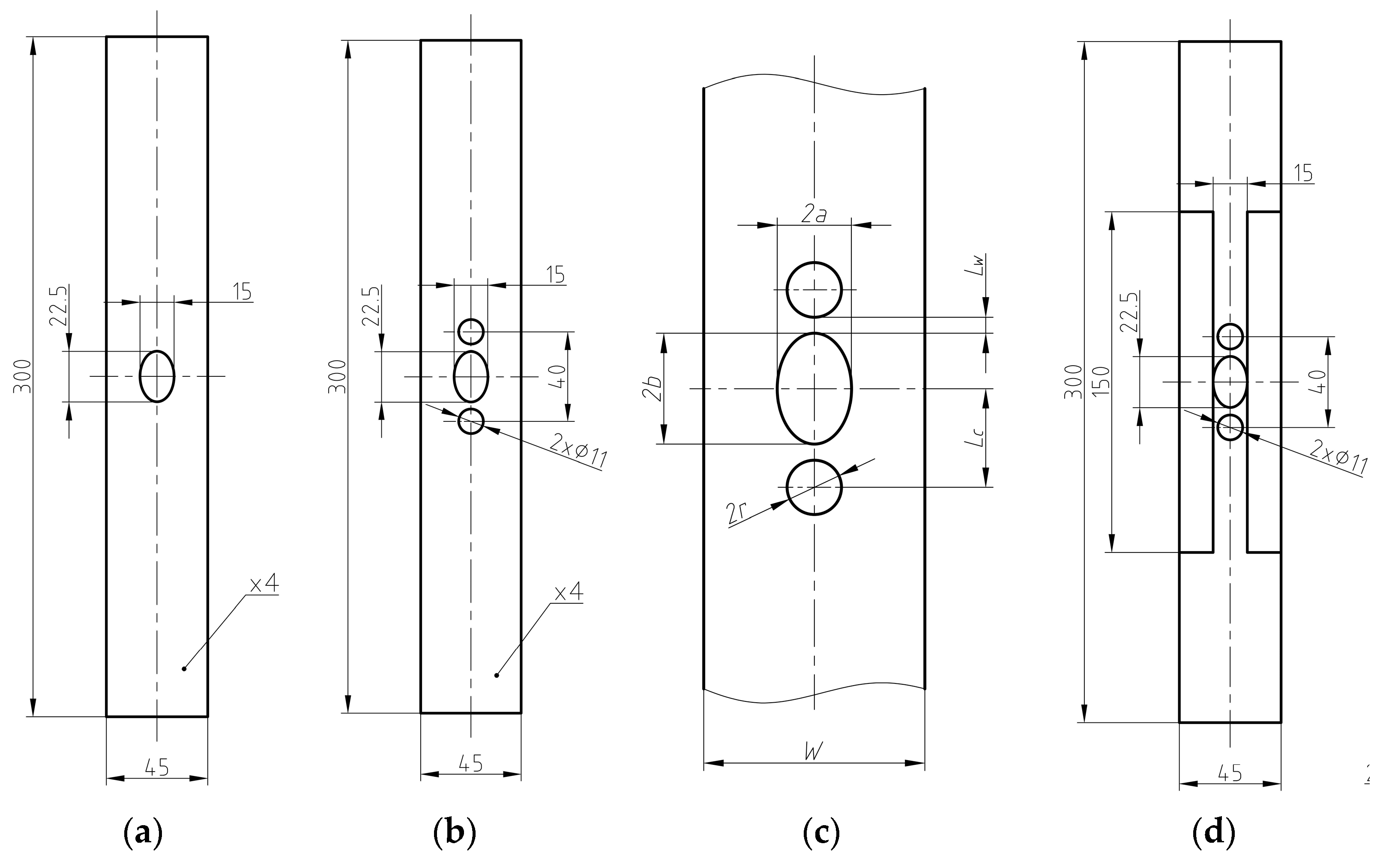
Figure 1. Geometries of samples: (a) with single elliptical opening; (b) with two circular stress relief holes; (c) designation of geometrical variables; (d) with two circular stress relief holes and reinforced by composite overlays.
Applsci 15 11194 g001
Figure 2. Photographs of tested specimens: (a) with single elliptical opening; (b) with elliptical opening and two circular relief holes; (c) test stand.
Applsci 15 11194 g002
Figure 3. Model with boundary conditions and loads applied.
Applsci 15 11194 g003
Figure 4. Finite element mesh of part of model and with detailed denser mesh around cut holes.
Applsci 15 11194 g004
Figure 5. Architecture of neural network (example for circular and elliptical holes only, meaning without circular relief holes).
Applsci 15 11194 g005
Figure 6. Stress concentration factor values for different elliptical and circular openings.
Applsci 15 11194 g006
Figure 7. Dependency between Ktn and chosen parameters in search area.
Applsci 15 11194 g007
Figure 8. Contour map of dependency between Ktn and chosen parameters in search area.
Applsci 15 11194 g008
Figure 9. Distribution of σx stresses in MPa in (a) entire sample; (b) around elliptical hole; and (c) around circular hole.
Applsci 15 11194 g009
Figure 10. The design space samples and Ktn values for circular and elliptical holes.
Applsci 15 11194 g010
Figure 11. The relationship between design variables and stress concentration factors for elliptical and circular holes (blue colours indicate minimum values and red colours indicate maximum values).
Applsci 15 11194 g011
Figure 12. The relationship between design variables and Ktn for elliptical hole (blue colours indicate minimum values and red colours indicate maximum values).
Applsci 15 11194 g012
Figure 13. The design space samples for densified design space and Ktn values for circular and elliptical holes.
Applsci 15 11194 g013
Figure 14. The relationship between design variables and Ktn for elliptical hole in densified design space (blue colours indicate minimum values and red colours indicate maximum values).
Applsci 15 11194 g014
Figure 15. Influence of ANN parameters on accuracy of calculations—single circular hole: (a) influence of number of neurons in hidden layers and number of hidden layers on maximal error of Ktn; (b) variation in the MSE during the ANN learning process.
Applsci 15 11194 g015
Figure 16. Influence of ANN parameters on accuracy of calculations—single circular hole: (a) influence of number of neurons in hidden layers and size of training set on maximal error of Ktn and R2 parameter; (b) influence of number of neurons in hidden layers and size of training set on M S E erro.
Applsci 15 11194 g016
Figure 17. Influence of ANN parameters on accuracy of calculations: (a) influence of number of neurons in hidden layers and size of training set on M A P E error; (b) influence of number of neurons in hidden layers and number of epochs on M S E error.
Applsci 15 11194 g017
Figure 18. Influence of ANN parameters on accuracy of calculations—single circular hole: (a) influence of number of neurons in hidden layers and number of epochs on M A X error and R2 parameter; (b) influence of number of neurons in hidden layers and number of epochs on M A P E error.
Applsci 15 11194 g018
Figure 19. Influence of ANN parameters on accuracy of calculations—single elliptical hole: (a) influence of number of neurons in hidden layers and size of training set on M A X error and R2 parameter; (b) influence of size of training set on M A X error and R2 parameter for number of neurons {32, 16}.
Applsci 15 11194 g019
Figure 20. Influence of ANN parameters on accuracy of calculations—single elliptical hole: (a) influence of size of training set on M A X error and R2 parameter for number of neurons {64, 32}; (b) influence of size of training set on M A X error and R2 parameter for number of neurons {128, 64}.
Applsci 15 11194 g020
Figure 21. Influence of number of neurons in hidden layers and size of training set on M A P E error—single elliptical hole.
Applsci 15 11194 g021
Figure 22. M S E error as a function of the number of neurons in the first hidden layer: (a) M S E taken from the last epoch of training; (b) M S E evaluation based on the testing set.
Applsci 15 11194 g022
Figure 23. Value of the Ktn coefficient as a function of the input parameters (radius of the relief circular hole and the distance between axes of the elliptical and circular cut-outs): (a) input (numerical FEM results) data; (b) ANN prediction.
Applsci 15 11194 g023
Figure 24. The relative error in each point of the feasible range of the input parameters.
Applsci 15 11194 g024
Figure 25. Value of the Ktn coefficient as a function of the input parameters (radius of the relief circular hole and the distance between axes of the elliptical and circular cut-outs) for the updated range of the input parameters: (a) numerical data; (b) ANN prediction.
Applsci 15 11194 g025
Figure 26. The relative error in each point of the updated feasible range of the input parameters.
Applsci 15 11194 g026
Figure 27. Failure modes of tested specimens (a) with single elliptical opening; (b) with elliptical opening and two circular relief holes.
Applsci 15 11194 g027
Figure 28. Distribution of principal vertical εy strain (for tensile loading equal to 40 kN) calculated in DIC analyses in (a) specimen with elliptical opening; (b) specimen with elliptical opening and two circular relief holes.
Applsci 15 11194 g028
Figure 29. Distribution of principal stress σx for specimens reinforced by composite overlays: (a) specimen with elliptical opening; (b) specimen with elliptical opening and two circular relief holes.
Applsci 15 11194 g029
Figure 30. Influence of size of training set on accuracy of determination of Ktn: (a) average relative error; (b) maximal relative error.
Applsci 15 11194 g030
Figure 31. Influence of size of training set on accuracy of determination of radius and position of stress relief holes: (a) relative error for radius r determination; (b) relative error for distance LC determination.
Applsci 15 11194 g031
Table 1. Chemical composition of S235JR steel (in weight %).
MaterialCSiMnPSCuCrNiVMoN
S235JR [43]0.110.190.920.0220.0240.300.120.120.0040.030.0116
S235JR (Standards [44])0.19-1.500.0450.0450.600.340.47-0.140.014
Table 2. Mechanical properties of S235JR steel.
MaterialE
(GPa)
νYield Limit
(MPa)
Ultimate Tensile Strength
(MPa)
Elongation at Failure
(%)
S235JR [43]2100.334449233
S235JR (Standards [44])2100.3≥235360–510≥26
Table 3. List of experimental tests performed in study.
Specimen No.Sample GeometryTest TypeComments
1–3Notched—elliptical hole Fatigue, tensile Figure 1a and Figure 2a
4–6Notched—elliptical hole with two stress relief holes Fatigue, tensile Figure 1b and Figure 2b
Table 4. Input and output parameters of ANN.
Studied CaseInput Parameter (s)Output Parameter (s)
1. Circular holed/WKtn
2. Elliptical holea/b, a/WKtn
3. Elliptical hole with circular relief holesa/W, r/WKtn and 5 other quantities
Table 5. Selected results of simple search optimisation (for: a = 7.5 mm, b = 11.25mm, W = 45 mm).
No.r (mm)LC (mm)LW (mm)Ktn (Elliptical) σ X , M A X c i r c l e (MPa)
ValueSMXBValueSMXB
15.74918.5321.5331.68251.68251.67871.6788
25.68718.9822.0441.68061.68061.68031.6803
35.67219.0852.1631.68061.68061.68061.6805
45.59719.8823.0351.68791.68791.68791.6879
55.55119.9773.1761.68351.68351.68311.6831
65.51020.2603.5001.68551.68551.68371.6837
75.45820.7504.0421.68801.68801.68741.6874
8 (tested)5.50020.0003.2501.68791.68791.67601.6760
Table 6. Candidate sets for the optimal solution.
Samples SetHole DiameterLengthCircular HoleElliptical HoleDifference
2R (mm)LW (mm) σ X , M A X c i r c l e (MPa)Ktn(%)
19.84.31.5821.7509.6
27.812.61.6671.8208.4
36.017.11.6841.8679.8
410.67.31.7211.7170.3
511.42.41.6801.6890.5
Table 7. Candidate sets for the optimal solution for densified design space.
Samples SetHole DiameterLengthCircular HoleElliptical HoleDifference
2r [mm]LW (mm) σ X , M A X c i r c l e (MPa)Ktn(%)
110.23.11.5821.7409.1
28.69.11.6151.7897.2
39.86.21.6341.7466.4
410.44.81.6471.7234.4
58.210.81.6311.8059.6
Table 8. Candidate sets for the optimal solution for densified design space with minimalisation of difference between Ktn for circular and elliptical holes.
Samples SetHole DiameterLengthCircular HoleEllitptical HoleDifference
2r [mm]LW (mm) σ X , M A X c i r c l e (MPa)Ktn(%)
19.611.31.7431.7681.4
29.8131.7901.7731.0
3109.61.7251.7471.3
410.29.91.7511.7420.5
510.68.21.7401.7201.1
Table 9. Optimal solution to the problem.
Minimal Value of KtnOptimal Radius r of Hole (mm)Optimal Distance LC (mm)
Numerical study1.6825.64319.185
Sub-variant 11.7194.80017.184
Sub-variant 21.7025.59018.910
Table 10. Fatigue life of tested specimens (r = 5.5 mm, LW = 3.25 mm).
NoSpecimen Type Eadh
(GPa)
KtnNf (Cycles)Nf,avg (Cycles) Standard   Dev . · 10 3 (Cycles)
1–3With singular elliptical holeExp.-1.908
(theoretical)
1.922
(FEM)
41,234, 52,516, 62,3065201810.55
4–6With elliptical hole with two circular relief holesExp.-1.68884,652, 91,987, 102,910931839.15
-With elliptical hole strengthened by composite overlaysFEM0.3551.790---
FEM0.5901.787---
FEM3.6001.779---
-With elliptical hole with two circular relief holes strengthened by composite overlaysFEM0.3551.596---
FEM0.5901.594---
FEM3.6001.587---
Table 11. List of optimal configurations obtained using different methods.
MethodScaleOptimal Decision Variables (mm)Ktn
r (mm)LW (mm)LC (mm)
Simple-search method (SSM)Global5.6722.16319.0851.6806
5.6872.04418.9821.6806
Parametric optimisation (Ansys APDL- PO)Global5.6922.00118.9441.6807
Local5.5513.17619.9771.6835
Goal-driven optimisation (GDO) (Ansys Workbench)Global5.72.419.351.689
Local5.24.821.251.723
ANN—macroGlobal4.8001.13417.1841.7185
Local4.5763.00218.8281.7270
ANN—localGlobal5.5902.07018.9101.7020
Local5.4863.00019.7361.7029
Tested -5.503.2520.001.6879
Specimen with singular elliptical opening ---1.908
Table 12. Comparison of applied optimisation techniques.
SSMAPDL-POGDOANN
Precision in global optimum searchvery highmoderatemoderatemoderate
Computational timevery highhighhigh
  • high (FEM analyses)
  • low—ANN calculations
Sensitivity for stacking in local minimumnot applicablehighlownot applicable
Number of analyses requiredvery highhighmoderatemoderate
Sensitivity for input datalowhighlowmoderate
Practical applicabilitylowmoderatehighhigh
Disclaimer/Publisher’s Note: The statements, opinions and data contained in all publications are solely those of the individual author(s) and contributor(s) and not of MDPI and/or the editor(s). MDPI and/or the editor(s) disclaim responsibility for any injury to people or property resulting from any ideas, methods, instructions or products referred to in the content.