Design of the Front Electrode Patterns of Solar Cells Using Geometry-Driven Optimization Method Based on Wide Quadratic Curves

Abstract

Enhancing solar cell performance is effectively attainable through optimization of the front electrode layout. This research tackles the electrode design problem via a geometry-driven optimization framework to discover high-efficiency front electrode patterns. The introduced methodology employs wide quadratic curves for representing the electrode geometry, wherein both the interpolation points and the widths of these curves function as design variables. Two solar cell configurations are utilized to test the optimization technology. In contrast to traditional shape optimization, the current strategy provides enhanced design flexibility, promoting novel and high-performance electrode configurations. Key parameters analyzed encompass the initial geometry, the count of wide quadratic curves, mesh resolution, and the size of the solar cell. Results demonstrate that the presented approach constitutes a viable and efficient design pathway for elevating solar cell operation. The performance of solar cells optimized using this technology outperforms those processed with a modified Solid Isotropic Material with Penalization (SIMP) approach. Furthermore, relative to typical H-pattern electrode grids, the optimized layouts not only achieve superior efficiency but also considerably minimize the consumption of electrode materials.

1. Introduction

As global energy demands continue to rise, the pursuit of clean and efficient energy sources is becoming increasingly critical. Solar power, an abundant and renewable energy resource, offers a viable solution to address these growing energy challenges. Solar cells, which directly convert sunlight into electricity, play a central role in harnessing this potential. Currently, the conversion efficiency of commercially available solar cells lags behind that achieved in laboratory settings. This discrepancy arises primarily due to the larger size of mass-produced solar cells, where the trade-off between resistive and shading losses becomes more pronounced [1]. Enhancing solar cell performance while reducing manufacturing costs remains a key focus for ongoing research and technological development [2,3,4,5].

A solar cell functions as a diode-like electronic component that transforms light directly into electricity. Its typical structure comprises a semiconductor layer enclosed between a front conductive layer (consisting of the front electrode grid and transparent conductive oxide (TCO) layer) and a back electrode layer (Figure 1). The front electrode grid, usually made from highly conductive metal materials, contains busbars and multiple fingers to minimize resistive losses within the solar cell. Although widening this grid can further decrease resistance loss, it simultaneously leads to an increase in shading loss.

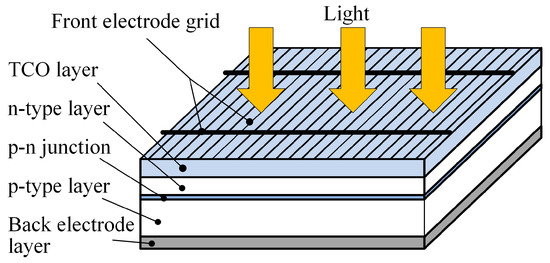
Figure 1. Typical solar cell configuration.

Figure 2 qualitatively illustrates the resistance loss, shading loss, total loss, and the quantity of front electrode material utilized on the solar cell’s surface. A trade-off exists between resistance and shading losses, with the total loss attaining a minimum at the balance point. Moreover, for a fixed amount of front electrode material, adjusting the shape and size of the electrode grid can further decrease resistance loss, as indicated by the gray region near the black dashed line in Figure 2. Consequently, optimizing the shape and size of the electrode grid enables minimization of the total loss in solar cells [6].

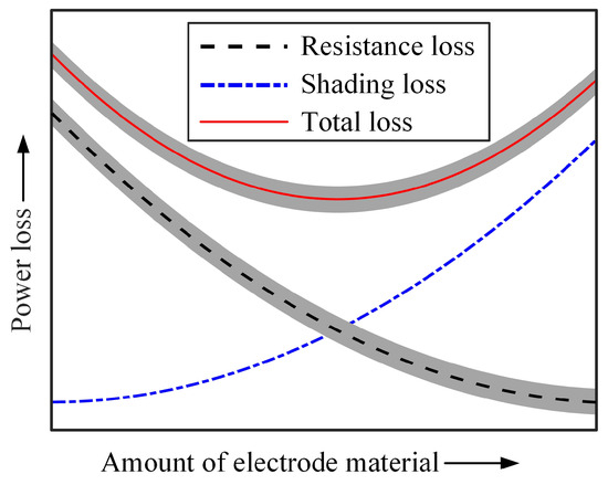
Figure 2. The series resistance loss, shading loss, and total loss in relation to the usage of front electrode material.

Significant research efforts have focused on optimizing the front electrode design for solar cells in the past. Green et al. [7] introduced a relative power loss model that identifies optimal grid parameters by minimizing total relative power loss. Djeffal et al. [8] developed an optimization approach using a genetic algorithm and applied it to two distinct electrode patterns. Li et al. [9] proposed a hybrid finite-element–genetic algorithm strategy for electrode design and validated its efficacy across two solar cell configurations. While these contributions have enhanced conversion efficiency to some degree, they confine the electrode to predetermined shapes, such as the H-pattern, thereby limiting both design freedom and potential performance improvements [10,11].

Topology optimization (TO) is a numerical method used to distribute material optimally in a predefined design domain, subject to given load conditions, constraints, and performance goals [12,13,14]. Unlike size or shape optimization, TO permits arbitrary material distribution, enabling the generation of high-performance configurations unattainable through conventional methods [15,16,17]. Gupta et al. [18] applied TO to design front electrode patterns for solar cells, demonstrating that the method can produce complex, non-traditional electrode geometries. Their work also extended to free-form and concentrated photovoltaic cells using the same optimization technology [19,20,21]. However, the resulting designs did not surpass traditional patterns in performance. This limitation stems from the use of the Solid Isotropic Material with Penalization (SIMP) method, which suffers from intermediate densities, blurred boundaries, and mesh dependency [22,23,24]. These issues hinder the translation of optimized results into practical computer-aided design (CAD) models [25].

To address the limitations of SIMP-based approaches and achieve superior electrode configurations, this paper introduces a geometry-driven optimization method utilizing the wide quadratic curve for front electrode pattern design. The geometry-driven optimization method adopts a processing approach similar to the topology optimization methods used in existing literature [26,27]. The structure of this paper is organized as follows: Section 2 outlines the solar cell architecture and presents the corresponding finite element model. Section 3 details the electrode pattern representation scheme, formulates the optimization objective function, and discusses sensitivity analysis along with the strategy for updating design variables. Numerical examples are provided in Section 4 to validate the effectiveness of the proposed methodology, and concluding remarks are summarized in Section 5.

2. Model of Solar Cells

2.1. Solar Cell Operation

Under photo-illumination, the semiconductor layer of the solar cell generates photocurrent. The current is collected by both the front conductive and back electrode layers, which then channel it to neighboring solar cells or an external circuit. Owing to the diode-like characteristics of a solar cell, it is often modeled using a single-diode equivalent circuit model [28], as illustrated in Figure 3. According to this model, the output behavior of the solar cell can be mathematically described by the following equation

$$I=I_{\mathrm{L}}-I_0\left(\exp \left({\displaystyle \frac{q\left(V+I{R}_{\mathrm{s}}\right)}{AKT}}\right)-1\right)-{\displaystyle \frac{\left(V+I{R}_{\mathrm{s}}\right)}{R_{\mathrm{sh}}}}$$

(1)

where I is the current, $I_{\mathrm{L}}$ is the photo-illumination current, $I_0$ is the reverse bias current, q is the electric charge, V is the voltage, $R_{\mathrm{s}}$ is the series resistance, $R_{\mathrm{sh}}$ is the shunt resistance, A is the diode ideality factor, K is the Boltzmann constant, and T is the absolute temperature.

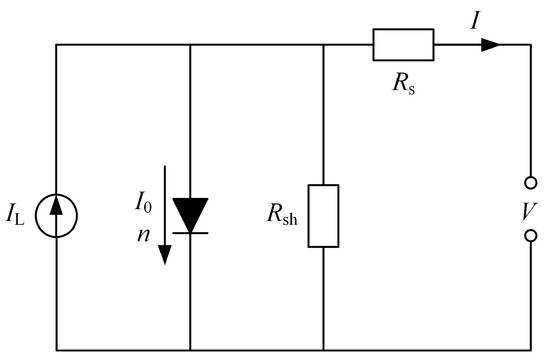
Figure 3. Equivalent circuit for a solar cell.

Owing to the significantly higher electrical conductivity of the front conductive and back electrode layers relative to the semiconductor layer, the photocurrent generated flows vertically toward the solar cell’s surface. It is then collected and conveyed either to an adjacent cell or an external load. This allows the solar cell to be represented by a two-dimensional model, as depicted in Figure 4. In this study, the front electrode is represented using a wide quadratic curve.

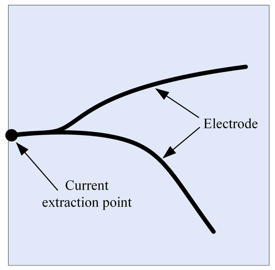
Figure 4. Schematic diagram of the front surface of solar cell.

2.2. Finite Element Model of Solar Cells

The limited conductivity of the front conductive layer leads to spatial variations in operating voltage and current density across the solar cell. To characterize the distribution of operating voltage and current density, a two-dimensional finite element model is employed, where each discrete element is used to describe an independent unit solar cell. The electrical performance of each unit solar cell can be described by

$$I_{\mathrm{e}}=\left\{J_{\mathrm{L}}^{*}-{\displaystyle \frac{1}{4}}\sum _{i=1}^4\left(J_0^{*}\left(\exp \left({\displaystyle \frac{q{u}_i}{A^{*}KT}}\right)-1\right)\right)-{\displaystyle \frac{u_i}{R_{\mathrm{sh}}^{*}}}\right\}{A}_{\mathrm{e}}$$

(2)

where $I_{\mathrm{e}}$ is the net current of the unit solar cell, $J_{\mathrm{L}}^{*}$ is the photo-illumination current density of the unit solar cell, $J_0^{*}$ is the reverse bias current density of the unit solar cell, $A^{*}$ is the diode ideality factor, $R_{\mathrm{sh}}^{*}$ is the shunt resistance, $u_i$ is the operating voltage at each corner position of the unit solar cell, and $A_{\mathrm{e}}$ is the area of the unit solar cell. The sum of the current of all unit solar cells is the current value of the entire solar cell.

The front electrode partially obstructs incident sunlight, thereby inducing a shading effect. Accounting for this phenomenon, the electrical behavior of each unit solar cell can be reformulated as

$$I_{\mathrm{e}}=\left\{J_{\mathrm{L}}^{*}\left(1-x_{\mathrm{e}}\right)-{\displaystyle \frac{1}{4}}\sum _{i=1}^4\left(J_0^{*}\left(\exp \left({\displaystyle \frac{q{u}_i}{A^{*}KT}}\right)-1\right)\right)-{\displaystyle \frac{u_i}{R_{\mathrm{sh}}^{*}}}\right\}{A}_{\mathrm{e}}$$

(3)

where $x_{\mathrm{e}}$ is the area proportion of the front electrode occupying the unit solar cell.

The distribution characteristics of the electrical potential on the surface of a solar cell can be described by a Poisson equation for electrical conductivity as

$$\sigma {\nabla }^{2}u={\displaystyle \frac{\partial \rho }{\partial t}}$$

(4)

where u is the electrical potential, and $\rho$ is the enclosed charge density. After the finite element discretization of Equation (4), the matrix equation for the solar cell can be written as

$$\mathbf{CU}=\mathbf{I}$$

(5)

where $\mathbf{C}$, $\mathbf{U}$, and $\mathbf{I}$ are the global conductivity matrix, voltage vector, and current vector, respectively. For detailed information on the finite element model of solar cells, please refer to [18]. Equation (1) shows that there is a nonlinear relationship between current and voltage, so Equation (5) cannot be solved directly. Thus, we rewrite Equation (5) in a residual form as

$$\mathbf{R}\left(\mathbf{U}\right)=\mathbf{CU}-\mathbf{I}=\mathbf{0}$$

(6)

where $\mathbf{R}$ is the residual. Equation (6) can be solved using the Newton–Raphson method.

3. Geometry-Driven Optimization Formulation

3.1. Geometric Representation Scheme

The goal of the front electrode pattern optimization is to identify an optimal electrode layout that maximizes solar cell efficiency. This study employs a set of wide quadratic curve components to represent the electrode pattern. Similar to conventional Moving Morphable Component (MMC)-based approaches, the optimal configuration is attained through rational arrangement of the positions and dimensions of components [29,30,31].

In this study, we use a set of wide quadratic curves to represent the moving morphable components, as illustrated in Figure 5. To build the wide quadratic curve, we use a quadratic curve as the central skeleton, and the shape of the quadratic curve is controlled by three interpolating points, denoted as $p_i\left(x_i,y_i\right)\left(i=1,2,3\right)$. The width of the wide quadratic curve is set to 2r, with r also serving as a design variable. Therefore, the shape and width of the nth wide quadratic curve are fully described by the following vector:

$${\mathbf{d}}_n={\left[x_{n1},y_{n1},x_{n2},y_{n2},x_{n3},y_{n3},r_n\right]}^{\mathrm{T}}$$

(7)

where $r_n$ is the half-width of the nth wide quadratic curve.

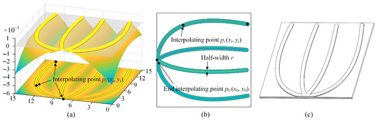
Figure 5. Four wide quadratic curves present the underlying idea: (a) geometric description function of the wide quadratic curves; (b) geometry structure of the electrode corresponding to the wide quadratic curves; (c) three-dimensional structural diagram of the electrode.

Accordingly, when the front electrode pattern comprises N wide quadratic curves, its geometry configuration is fully defined by the following vector:

$$\mathbf{d}={\left[{\mathbf{d}}_1,{\mathbf{d}}_2,\dots ,{\mathbf{d}}_n,\dots ,{\mathbf{d}}_N\right]}^{\mathrm{T}}$$

(8)

In accordance with Kirchhoff’s law, all the currents must converge at the current extraction point, necessitating that every current-collecting electrode connect to this location. Reflecting this principle, one end of the interpolating point of each quadratic curve is fixed at the current extraction point, as depicted in Figure 5. Consequently, the coordinates of this fixed endpoint for the nth curve are predefined, allowing the design variable vector ${\mathbf{d}}_n$ to be divided into two distinct parts

$${\mathbf{d}}_n=\left[\begin{array}{c}{{\mathbf{d}}_n}^{\mathrm{p}}\\ {{\mathbf{d}}_n}^{\mathrm{f}}\end{array}\right]$$

(9)

whrere ${{\mathbf{d}}_n}^{\mathrm{p}}={\left[x_{n1},y_{n1}\right]}^{\mathrm{T}}$ and ${{\mathbf{d}}_{\mathrm{n}}}^{\mathrm{f}}={\left[x_{n2},y_{n2},x_{n3},y_{n3},r_n\right]}^{\mathrm{T}}$ are the predefined and free design variables, respectively.

The coordinates of any point on a quadratic curve can be formulated using the following parametric functions:

$$\left\{\begin{array}{c}x\left(t\right)={\displaystyle \sum _{i=1}^3}{x}_i{l}_i\left(t\right)\\ y\left(t\right)={\displaystyle \sum _{i=1}^3}{y}_i{l}_i\left(t\right)\end{array}\right.$$

(10)

where $x_i$ and $y_i$ are the coordinates of the ith interpolating point in the x and y directions, respectively. t is an intrinsic parameter, and its value range is from 0 to 1. $l_i\left(t\right)$ is the quadratic Lagrange interpolation basis function. The expression of $l_i\left(t\right)$ is as follows:

$$\left\{\begin{array}{c}{l}_1\left(t\right)={\displaystyle \frac{\left(t-0.5\right)\left(t-1\right)}{\left(0-0.5\right)\left(0-1\right)}}\hfill \\ l_2\left(t\right)={\displaystyle \frac{\left(t-0\right)\left(t-1\right)}{\left(0.5-0\right)\left(0.5-1\right)}}\hfill \\ l_3\left(t\right)={\displaystyle \frac{\left(t-0\right)\left(t-0.5\right)}{\left(1-0\right)\left(1-0.5\right)}}.\hfill \end{array}\right.$$

(11)

The nth wide quadratic curve is determined using a function ${\varphi }_{\mathrm{m}}$ as

$${\varphi }_{\mathrm{m}}=r_{\mathrm{m}}-\left|p\left(x,y\right)-\left(x_{\mathrm{m}}\left(t\right),y_{\mathrm{m}}\left(t\right)\right)\right|$$

(12)

where $\left|p\left(x,y\right)-\left(x_{\mathrm{m}}\left(t\right),y_{\mathrm{m}}\left(t\right)\right)\right|$ represents the shortest distance from point $p(x,y)$ to the quadratic curve.

3.2. Defining Objective Function

The aim of geometry-driven optimization in this context is to identify the best front electrode configuration that maximizes the solar cell’s output power. Since all generated currents must pass through the current extraction point, the objective function f is formulated as follows:

$$f=P_{\mathrm{out}}=V_{\mathrm{op}}{A}_{\mathrm{e}}\sum I_{\mathrm{e}}$$

(13)

where $V_{\mathrm{op}}$ is the operating voltage. Thus, the optimization problem to find the optimal front electrode pattern can be written as follows:

$$\begin{array}{c}\begin{array}{cc}\hfill \mathrm{Find}:& \mathbf{d}={\left[{\mathbf{d}}_1,{\mathbf{d}}_2,\dots ,{\mathbf{d}}_m,\dots ,{\mathbf{d}}_N,V_{\mathrm{op}}\right]}^{\mathrm{T}},\hfill \\ \hfill min:& f=-P_{\mathrm{out}}=-V_{\mathrm{op}}\sum I\mathrm{e},\hfill \\ \hfill \mathrm{s}.\mathrm{t}.:& \mathbf{CU}=\mathbf{I}.\hfill \end{array}\hfill \end{array}$$

(14)

where ${\left[{\mathbf{d}}_1,{\mathbf{d}}_2,\dots ,{\mathbf{d}}_n,\dots ,{\mathbf{d}}_N,V_{\mathrm{op}}\right]}^{\mathrm{T}}$ is the set of design variables. In this paper, we use gradient information-based methods to update the design variable.

3.3. Sensitivity Analysis

To facilitate gradient-based optimization, the sensitivities of the objective function are derived via adjoint analysis. The sensitivity of the objective function with respect to the design variables a is given by the following expression:

$$\begin{array}{c}{\displaystyle \frac{\partial \tilde{f}\left(a\right)}{\partial a}}={\displaystyle \frac{\partial }{\partial a}}\left(f+{\lambda }^{\mathrm{T}}\left(\mathbf{CU}-\mathbf{I}\right)\right)\hfill \\ ={\displaystyle \frac{\partial f}{\partial a}}+{\left[\begin{array}{c}{\lambda }_f\\ {\lambda }_p\end{array}\right]}^{\mathrm{T}}{\displaystyle \frac{\partial }{\partial a}}\left(\left[\begin{array}{cc}{\mathbf{C}}_{ff}& {\mathbf{C}}_{fp}\\ {\mathbf{C}}_{pf}& {\mathbf{C}}_{pp}\end{array}\right]\left[\begin{array}{c}{\mathbf{U}}_f\\ {\mathbf{U}}_p\end{array}\right]-\left[\begin{array}{c}{\mathbf{I}}_f\\ {\mathbf{I}}_p\end{array}\right]\right)\hfill \end{array}$$

(15)

where $\lambda$ is a Lagrange multiplier. The subscript symbols f and p are related to the free points and predefined points, respectively. ${\mathbf{U}}_p$ is the operating voltage (for more details on this aspect, please refer to [18]).

3.4. Update Design Variable

The design variables for each wide quadratic curve are updated via the Method of Moving Asymptotes (MMA), an iterative algorithm utilizing sensitivity information to address general nonlinear optimization problems [32]. As a widely adopted optimizer, MMA has been extensively applied in geometry-driven optimization. In this study, the iterative process terminates when the objective function value over the previous five steps remains within a tolerance of 0.00001% of the current value, or when a predefined maximum number of iterations is attained.

4. Results and Discussions

To validate the effectiveness of the proposed approach, two solar cell configurations are employed (Figure 6). The first is a side-contact cell (Figure 6a), with its left-side midpoint—functioning as the current extraction point—maintained at voltage $V_{\mathrm{op}}$. The other is a pin-up module (PUM) solar cell (Figure 6b), with its centroid serving as the current extraction point and also maintained at voltage $V_{\mathrm{op}}$. Following the boundary conditions, one interpolation point on each quadratic curve is anchored at the corresponding current extraction point in both designs.

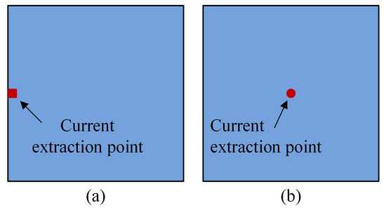
Figure 6. Two different solar cell configurations: (a) side-contact solar cell, (b) PUM solar cell.

For the cases, the voltage–current density relationship of a solar cell is adopted as follows

$$j=310-0.006\left(exp\left(16.4V\right)\right)$$

(16)

In Equation (16), the units of V and j are volts and $\mathrm{A}·{\mathrm{m}}^{-2}$, respectively. The thickness and the conductivities of the TCO layer are 200 nm and ${10}^5\mathrm{S}·{\mathrm{m}}^{-1}$, respectively. The thickness and the conductivities of the front electrode are 10 $\mathrm{\mu }$m and ${10}^7\mathrm{S}·{\mathrm{m}}^{-1}$, respectively. The above parameters are consistent with those in the literature [18].

The efficiency ($\eta$) of solar cells is calculated as

$$\eta ={\displaystyle \frac{P_{\mathrm{out}}/\phantom{P_{\mathrm{out}}{A}_{\mathrm{c}}}{A}_{\mathrm{c}}}{p_{\mathrm{in}}}}\times 100\%$$

(17)

where $P_{\mathrm{out}}$ and $A_{\mathrm{c}}$ are the output power and area of the solar cell, respectively. $P_{\mathrm{in}}$ is the input power density, which is assumed to be 1000 $\mathrm{W}·{\mathrm{m}}^{-2}$.

4.1. Dependency on the Initial Geometry Patterns

To evaluate the influence of the initial geometry pattern on the optimized results, the side-contact solar cell is analyzed under five distinct initial configurations. The cell dimensions are set to $15\mathrm{mm}\times 15\mathrm{mm}$, with a discretization of $100\times 100$ elements in the design domain for all cases. Each initial electrode pattern is represented using six wide quadratic curves, each having a width set to 0.02 times the design domain length. Accounting for constraints in electrode printing technology, the minimum width of all curves is fixed at 50 $\mathrm{\mu }$m across all cases.

Figure 7 displays the five initial geometries, with their corresponding optimized configurations illustrated in Figure 8. The conversion efficiency ($\eta$) and operating voltage ($V_{\mathrm{op}}$) for each case are provided in Table 1. Despite considerable variation in the initial geometries, the optimized electrodes consistently distribute extensively to maximize current collection. Table 1 indicates only minor differences in both conversion efficiency and operating voltage across the five cases. Consequently, subsequent analysis employs a manually defined initial geometry for the front electrode pattern.

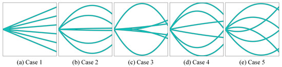
Figure 7. The initial geometries of the side-contact solar cells.

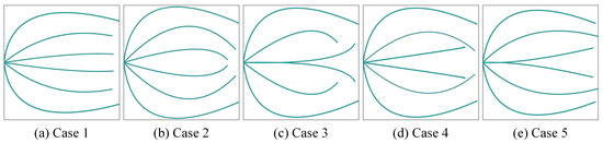
Figure 8. The optimized geometries of the side-contact solar cells.

Table 1. Resulting values of the optimized side-contact solar cell with different initial geometries.

	Case 1	Case 2	Case 3	Case 4	Case 5
$\eta$ (%)	13.607	13.614	13.569	13.586	13.581
$V_{\mathrm{op}}\left(\mathrm{V}\right)$	0.507	0.508	0.507	0.507	0.505

Figure 9 shows the convergence history of the solar cell conversion efficiency and the changing history of the geometric description functions for the wide quadratic curves of case 1 in Figure 7. It can be seen that the efficiency rises quickly with increasing iteration count and stabilizes after approximately 800 generations, with little further improvement. Several intermediate patterns of the front electrode are also displayed in the same figure. Initially, the electrode grids appear clustered together; as the optimization proceeds, they become progressively more dispersed. The process terminates once the specified maximum number of iterations is attained.

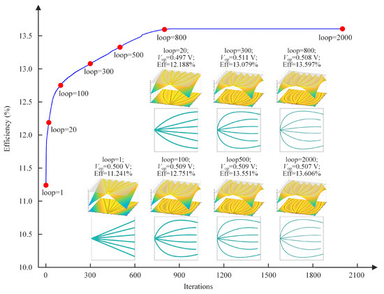
Figure 9. Convergence history of the solar cell conversion efficiency and changing history of the front electrode pattern of case 1 in Figure 7.

4.2. Dependency on the Number of Wide Quadratic Curves

Building upon the analysis in Section 4.1, the influence of the number of wide quadratic curves ($NWQC$) on solar cell conversion efficiency is further investigated. Six cases are considered, with NWQC values set to 4, 6, 8, 10, 12, and 14. All cases maintain the same side-contact solar cell dimensions and finite element discretization as specified in Section 4.1.

The initial geometries are illustrated in Figure 10, with the corresponding optimized configurations presented in Figure 11. Conversion efficiency and operating voltage for the six cases are summarized in Table 2. Results indicate that efficiency initially rises and then gradually declines as the number of wide quadratic curves increases. Peak efficiency of 13.666% occurs at ten curves. For a $15\mathrm{mm}\times 15\mathrm{mm}$ side-contact solar cell, considering both optimization speed and performance, approximately ten wide quadratic curves represent an appropriate configuration.

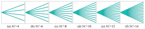
Figure 10. The initial geometries of the side-contact solar cells with different numbers of curves.

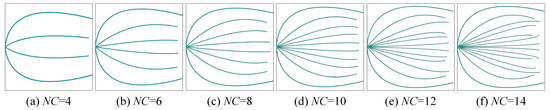
Figure 11. The optimized geometries of the side-contact solar cells with different numbers of curves.

Table 2. Resulted values of the optimized side-contact solar cell with different numbers of curves.

$\mathit{NWQC}$	4	6	8	10	12	14
$\eta$ (%)	13.439	13.607	13.653	13.666	13.661	13.653
$V_{\mathrm{op}}\left(\mathrm{V}\right)$	0.502	0.507	0.509	0.510	0.510	0.510

4.3. Dependency on the Mesh Resolution

Here, the influence of mesh resolution on the front electrode layouts and conversion efficiency is investigated for both side-contact and PUM solar cells using four different mesh densities. The solar cell dimensions remain $15\mathrm{mm}\times 15\mathrm{mm}$ for all cases, with element counts of $100\times 100$, $200\times 200$, $300\times 300$, and $400\times 400$, respectively. The initial geometries for both solar cells are illustrated in Figure 12.

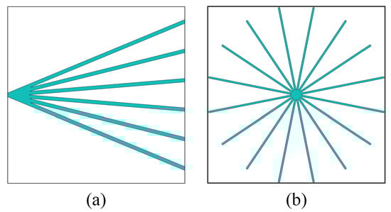
Figure 12. The initial geometries of the side-contact and PUM solar cell: (a) side-contact solar cell; (b) PUM solar cell.

Figure 13 and Figure 14 present the optimized designs for the side-contact and PUM solar cells, respectively, while the associated conversion efficiencies are listed in Table 3. Although the optimized geometries vary across mesh resolutions for each solar cell configuration, the differences in conversion efficiency remain minor. Notably, all cases exhibit higher efficiency than those reported by Gupta et al. [18], as also documented in Table 3.

Figure 13. The optimized geometries of the side-contact solar cells with different mesh resolutions.

Figure 14. The optimized geometries of the PUM solar cells with different mesh resolutions.

Table 3. Efficiency of the optimized side-contact and PUM solar cell with different mesh resolutions.

	Efficiency	Case a	Case b	Case c	Case d
Side-contact solar cell	$\eta$ (%) $\eta$ (%) [18]	13.607 12.46	13.598 12.98	13.596 13.02	13.589 13.04
PUM solar cell	$\eta$ (%) $\eta$ (%) [18]	13.886 12.84	13.916 13.11	13.906 13.16	13.894 13.43

4.4. Effect of Solar Cell Size

To assess how the physical dimensions of solar cells affect the optimized electrode pattern and conversion efficiency, an analysis is conducted on PUM solar cells with four distinct sizes. The dimensions of the four cases are $15\mathrm{mm}\times 15\mathrm{mm}$, $30\mathrm{mm}\times 30\mathrm{mm}$, $60\mathrm{mm}\times 60\mathrm{mm}$, and $90\mathrm{mm}\times 90\mathrm{mm}$, respectively. A consistent finite element size is maintained across all cases by discretizing the domains into $100\times 100$, $200\times 200$, $400\times 400$, and $600\times 600$ elements, respectively. The front electrode patterns are represented using 16, 32, 40, and 48 wide quadratic curves for the four cases.

Figure 15 shows the initial geometries for the four PUM solar cell cases, with their optimized geometries displayed in Figure 16. Table 4 summarizes the conversion efficiency, operating voltage, and front electrode material coverage ratio (CR) for all cases. Results indicate that conversion efficiency declines as solar cell size increases, which can be attributed to the greater average distance from current generation sites to the current extraction point, elevating resistive losses. Compensating by widening the electrode grid reduces resistive loss but increases shading loss, exacerbating the trade-off between these losses in large-sized cells. Additionally, all four cases exhibit higher conversion efficiency and operating voltage than those reported by Gupta et al. [18], as also noted in Table 4. It is important to note that the quantity of wide quadratic curves allocated in this study was chosen arbitrarily and does not represent an optimized value. For large-sized PUM solar cells, the quantity of curves is insufficient, and increasing the number could further enhance performance.

Figure 15. The initial geometries of the PUM solar cells with different sizes.

Figure 16. The optimized geometries of the PUM solar cells with different sizes.

Table 4. Results of the PUM solar cell with different sizes.

Cell Sizes	$15\mathbf{mm}\times 15\mathbf{mm}$	$30\mathbf{mm}\times 30\mathbf{mm}$	$60\mathbf{mm}\times 60\mathbf{mm}$	$90\mathbf{mm}\times 90\mathbf{mm}$
$\eta$ (%)	13.886	13.408	12.480	11.422
$V_{\mathrm{op}}\left(\mathrm{V}\right)$	0.512	0.507	0.489	0.468
$\mathrm{CR}$ (%)	3.583	6.171	7.875	9.977
$\eta$ (%) [18]	12.84	12.36	11.54	10.70
$V_{\mathrm{op}}\left(\mathrm{V}\right)$ [18]	0.502	0.495	0.481	0.466

4.5. Preliminary Comparison with H-Parttern Electrode

Currently, the H-pattern electrode remains the most widely used electrode grid configuration. This section compares this conventional electrode grid design with electrode layouts represented by wide quadratic curves. As depicted in Figure 17, a typical H-pattern electrode pattern consists of a busbar and a set of parallel fingers, where the current extraction point is located at the mid-position of the left boundary. The design parameters for the H-pattern electrode include the busbar width, finger width, and the total number of fingers. The solar cell’s model and material properties are consistent with those applied in the above analysis.

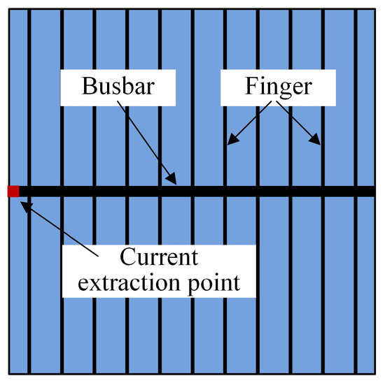
Figure 17. Typical H-pattern electrode grid.

Four solar cell sizes were investigated. The dimensions of the four cases are $15\mathrm{mm}\times 15\mathrm{mm}$, $20\mathrm{mm}\times 20\mathrm{mm}$, $25\mathrm{mm}\times 25\mathrm{mm}$, and $35\mathrm{mm}\times 35\mathrm{mm}$, respectively. The corresponding mesh resolutions for the four cases are set to $300\times 300$, $400\times 400$, $500\times 500$, and $700\times 700$, respectively.

For solar cells with the H-pattern front electrode, the optimized busbar width, finger width, and finger number are recorded in Table 5. For solar cells with the quadratic curve-shaped front electrode, the front electrode pattern is represented by 10, 16, 18, and 20 wide quadratic curves. The optimized electrode layouts are shown in Figure 18. The short-circuit current density ($J_{\mathrm{sc}}$), the open-circuit voltage ($V_{\mathrm{oc}}$), the current density ($J_{\mathrm{mp}}$) and voltage ($V_{\mathrm{mp}}$) at the maximum output power point, the fill factor ($FF$), the corresponding conversion efficiency, and the electrode material coverage ratio (CR) of the solar cells with the H-pattern and curve-shaped electrode are recorded in Table 6. The improvement in these parameters is also recorded in Table 6. From Table 6, it can be seen that compared with solar cells with the H-pattern electrode, all parameters of solar cells with the curve-shaped electrode have been improved. To better contextualize these results, we further emphasized the advantages of this method in terms of material savings and performance improvement. Specifically, although the absolute conversion efficiency gain may seem limited, the optimized front electrode patterns achieve a material coverage reduction of 16.677%, 8.891%, 18.041%, and 19.830%, while still relatively improving the conversion efficiency by 1.297%, 1.399%, 1.697%, and 1.852%. Furthermore, the enhancement in conversion efficiency becomes more pronounced as the solar cell size increases.

Table 5. The optimized busbar width, finger width, and finger number of the solar cell with the typical H-pattern front electrode.

Cell Size	Busbar Width $\left(\mathbf{\mu }\mathbf{m}\right)$	Finger Width $\left(\mathbf{\mu }\mathbf{m}\right)$	Finger Number
$15\mathrm{mm}\times 15\mathrm{mm}$	300.13	54.19	8
$20\mathrm{mm}\times 20\mathrm{mm}$	513.49	55.95	11
$25\mathrm{mm}\times 25\mathrm{mm}$	806.17	57.51	14
$35\mathrm{mm}\times 35\mathrm{mm}$	1536.99	60.76	20

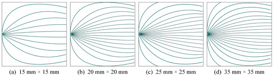
Figure 18. The optimized geometries of the side-contact solar cells with different sizes.

Table 6. Results of the side-contact solar cell with different electrode patterns.

Cell Sizes	$15\mathbf{mm}\times 15\mathbf{mm}$	$20\mathbf{mm}\times 20\mathbf{mm}$	$25\mathbf{mm}\times 25\mathbf{mm}$	$35\mathbf{mm}\times 35\mathbf{mm}$
$J_{\mathrm{sc}}$ ($\mathrm{A}·{\mathrm{m}}^{-2}$) (Curve-shaped)	301.062	298.480	297.288	293.437
$J_{\mathrm{sc}}$ ($\mathrm{A}·{\mathrm{m}}^{-2}$) (H-pattern)	298.085	295.600	293.326	289.643
Improvement in $J_{sc}$ ($\mathrm{A}·{\mathrm{m}}^{-2}$)	2.977	2.880	3.962	3.794
$V_{\mathrm{oc}}$ (V) (Curve-shaped)	0.6598	0.6592	0.6589	0.6579
$V_{\mathrm{oc}}$ (V) (H-pattern)	0.6592	0.6586	0.6580	0.6569
Improvement in $V_{oc}$ (V)	0.0006	0.0006	0.0009	0.0010
$J_{\mathrm{mp}}$ ($\mathrm{A}·{\mathrm{m}}^{-2}$) (Curve-shaped)	267.923	265.014	263.203	257.896
$J_{\mathrm{mp}}$ ($\mathrm{A}·{\mathrm{m}}^{-2}$) (H-pattern)	265.204	262.380	259.664	254.602
Improvement in $J_{mp}$ ($\mathrm{A}·{\mathrm{m}}^{-2}$)	2.719	2.634	3.539	3.294
$V_{\mathrm{mp}}$ (V) (Curve-shaped)	0.5100	0.5060	0.5008	0.4901
$V_{\mathrm{mp}}$ (V) (H-pattern)	0.5086	0.5040	0.4922	0.4879
Improvement in $V_{mp}$ (V)	0.0014	0.0020	0.0016	0.0022
$FF$ (%) (Curve-shaped)	68.785	68.156	67.290	65.475
$FF$ (%) (H-pattern)	68.649	67.929	67.153	65.288
Improvement in $FF$ (%)	0.136	0.227	0.137	0.187
$\eta$ (%) (Curve-shaped)	13.664	13.410	13.181	12.652
$\eta$ (%) (H-pattern)	13.489	13.225	12.961	12.422
Improvement in $\eta$ (%)	0.175	0.185	0.220	0.230
Relative improvement in $\eta$ (%)	1.297	1.399	1.697	1.852
$\mathrm{CR}$ (%) (Curve-shaped)	4.027	5.062	5.197	6.230
$\mathrm{CR}$ (%) (H-pattern)	4.833	5.556	6.341	7.771
Reduction in $\mathrm{CR}$ (%)	0.806	0.494	1.144	1.541
Relative reduction in $\mathrm{CR}$ (%)	16.677	8.891	18.041	19.830

In addition, the current density–voltage (J–V) curves of the solar cells with the H-pattern and curve-shaped electrode are depicted in Figure 19 to demonstrate the effectiveness of the electrode pattern optimized by using the proposed method. It can be seen from Figure 19 that for solar cells of the same size, solar cells with the curved-shaped electrode exhibit better performance compared with solar cells with the H-pattern electrode.

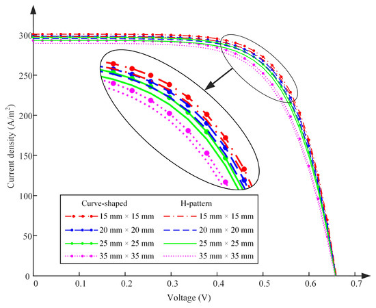
Figure 19. The J–V curves of the solar cells with the H-pattern and curve-shaped electrode.

Figure 20 shows the voltage and current density distribution of solar cells with different electrode patterns. From Figure 20, it can be seen that a considerable part of the voltage distribution diagram for solar cells with the H-pattern electrode is represented in dark red (higher operating voltage), while the voltage distribution diagram for solar cells with the curve-shaped electrode is relatively less represented in dark red. Correspondingly, in the case of the current density distribution in Figure 20, it can be seen that a considerable part of the current density diagram for solar cells with the H-pattern electrode is represented in blue (lower current density), while the current density diagram for solar cells with the curve-shaped electrode is relatively less represented in blue.

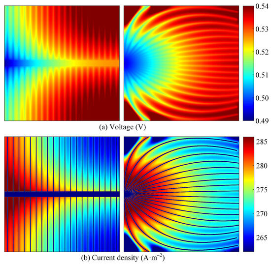
Figure 20. Voltage and current density distributions for solar cells with different electrode patterns.

5. Conclusions

Improving the performance of solar cells can be efficiently realized by optimizing the layout of the front electrode. This study applies a geometry-driven optimization method to enhance the electrode design, representing the electrode grid structure through a set of wide quadratic curves. The shape and size of each curve are determined by the coordinates of its interpolation points and its width. All design variables are optimized via the MMA.

The effectiveness of the introduced geometry-driven optimization method was confirmed through application to both side-contact and PUM solar cells. Results demonstrate its capability to produce complex and high-performance electrode patterns. Key factors examined include the initial geometry, quantity of wide quadratic curves, mesh resolution, and solar cell size. The results indicate that the initial layout and mesh resolution have minimal influence on solar cell performance, whereas increasing the number of curves appropriately could enhance the conversion efficiency. Conversely, larger solar cell dimensions lead to reduced solar cell performance.

Solar cells optimized using the proposed method exhibit enhanced performance relative to those designed with the conventional SIMP-based topology optimization method.

Relative to typical H-pattern electrodes, the quadratic curve-based design enhances solar cell performance while simultaneously significantly reducing the consumption of electrode materials. Moreover, as the size of solar cells increases, the improvement in solar cell conversion efficiency becomes more significant. This demonstrates the ability of the proposed method to balance performance enhancement with significant material savings.

The present work focuses on the macro-scale geometric optimization of the electrode, assuming an ideal electrical contact between the electrode and the semiconductor layer. A valuable extension would be to integrate a contact physics model that considers the work functions of the electrode and semiconductor materials, allowing for the prediction of potential barrier formation and its impact on carrier recombination and contact resistance. This would enable a multi-scale optimization of both the electrode pattern and material system to suppress potential barriers and improve solar cell performance.

References

- Green, M.A.; Dunlop, E.D.; Yoshita, M.; Kopidakis, N.; Bothe, K.; Siefer, G.; Hao, X.; Jiang, J.Y. Solar Cell Efficiency Tables (Version 65). Prog. Photovoltaics 2025, 33, 3–15. [Google Scholar] [CrossRef]
- Zhao, S.; Li, Q.; Sun, Y.; Wang, D.; Song, Q.; Zhou, S.; Li, J.; Li, Y. Application of multi-objective optimization based on Sobol sensitivity analysis in solar single-double-effect LiBr-H2O absorption refrigeration. Front. Energy 2025, 19, 69–87. [Google Scholar] [CrossRef]
- Han, A.; Wang, X.; Liu, X.; Huang, Y.; Meng, F.; Liu, Z. Improvement of Ga distribution in Cu(In, Ga)(S, Se)2 film by pretreated Mo back contact. Sol. Energy 2018, 162, 109–116. [Google Scholar] [CrossRef]
- Adrian, A.; Rudolph, D.; Willenbacher, N.; Lossen, J. Finger metallization using pattern transfer printing technology for c-Si solar cell. IEEE J. Photovolt. 2020, 10, 1290–1298. [Google Scholar] [CrossRef]
- Shen, W.; Zhao, Y.; Liu, F. Highlights of mainstream solar cell efficiencies in 2024. Front. Energy 2025, 19, 8–17. [Google Scholar] [CrossRef]
- Pingel, S.; Wenzel, T.; Göttlicher, N.; Linse, M.; Folcarelli, L.; Schube, J.; Hoffmann, S.; Tepner, S.; Lau, Y.C.; Huyeng, J.; et al. Progress on the reduction of silver consumption in metallization of silicon heterojunction solar cells. Sol. Energy Mater. Sol. Cells 2024, 265, 112620. [Google Scholar] [CrossRef]
- Green, M.A. Solar Cells: Operating Principles, Technology, and System Applications; Prentice-Hall, Inc.: Englewood Cliffs, NJ, USA, 1982. [Google Scholar]
- Djeffal, F.; Bendib, T.; Arar, D.; Dibi, Z. An optimized metal grid design to improve the solar cell performance under solar concentration using multiobjective computation. Mater. Sci. Eng. B-Adv. Funct. Solid-State Mater. 2013, 178, 574–579. [Google Scholar] [CrossRef]
- Li, K.; Yang, Z.; Zhang, X. Size optimization of the front electrode and solar cell using a combined finite-element-genetic algorithm method. J. Photonics Energy 2021, 11, 034502. [Google Scholar] [CrossRef]
- Nakano-Baker, O.; Boyd, C.; Cramer, C.; Brush, L.; MacKenzie, J.D. Isotropic Grids Revisited: A Numerical Study of Solar Cell Electrode Geometries. IEEE Trans. Electron. Devices 2022, 69, 3783–3790. [Google Scholar] [CrossRef]
- Li, K.; Wang, R.; Zhang, X.; Zhu, B.; Liang, J.; Yang, Z. Topology optimization of the front electrode patterns of solar cells based on moving wide Bezier curves with constrained end. Struct. Multidiscip. Optim. 2022, 65, 57. [Google Scholar] [CrossRef]
- Liang, J.; Zhang, X.; Zhu, B.; Zhang, H.; Wang, R. Topology Optimization Method for Designing Compliant Mechanism With Given Constant Force Range. J. Mech. Robot. 2023, 15, 1942–4302. [Google Scholar] [CrossRef]
- Wang, R.; Zhang, X.; Zhu, B.; Li, H.; Zhong, X.; Xu, N. A Topology-Optimized Compliant Microgripper With Replaceable Modular Tools for Cross-Scale Microassembly. IEEE-ASME Trans. Mechatron. 2024, 29, 2067–2078. [Google Scholar] [CrossRef]
- Zhang, W.; Li, D.; Zhou, J.; Du, Z.; Li, B.; Guo, X. A moving morphable void (MMV)-based explicit approach for topology optimization considering stress constraints. Comput. Meth. Appl. Mech. Eng. 2018, 334, 381–413. [Google Scholar] [CrossRef]
- Zhang, W.; Lai, Q.; Guo, X.; Youn, S.K. Topology optimization for the design of manufacturable piezoelectric energy harvesters using dual-moving morphable component method. J. Mech. Des. 2024, 146, 121701. [Google Scholar] [CrossRef]
- Zhang, W.; Zhang, S.; Youn, S.K.; Guo, X. Non-parametric geometry patching technique for MMC topology optimization. Struct. Multidiscip. Optim. 2024, 67, 77. [Google Scholar] [CrossRef]
- Zhu, B.; Wang, R.; Liang, J.; Lai, J.; Zhang, H.; Li, H.; Li, H.; Nishiwaki, S.; Zhang, X. Design of compliant mechanisms: An explicit topology optimization method using end-constrained spline curves with variable width. Mech. Mach. Theory 2022, 171, 104713. [Google Scholar] [CrossRef]
- Gupta, D.K.; Langelaar, M.; Barink, M.; van Keulen, F. Topology optimization of front metallization patterns for solar cells. Struct. Multidiscip. Optim. 2015, 51, 941–955. [Google Scholar] [CrossRef]
- Gupta, D.K.; Barink, M.; Galagan, Y.; Langelaar, M. Integrated Front-Rear-Grid Optimization of Free-Form Solar Cells. IEEE J. Photovolt. 2017, 7, 294–302. [Google Scholar] [CrossRef]
- Gupta, D.K.; Barink, M.; Langelaar, M. CPV solar cell modeling and metallization optimization. Sol. Energy 2018, 159, 868–881. [Google Scholar] [CrossRef]
- Gupta, D.K.; Langelaar, M.; Barink, M.; van Keulen, F. Optimizing front metallization patterns: Efficiency with aesthetics in free-form solar cells. Renew. Energy 2016, 86, 1332–1339. [Google Scholar] [CrossRef]
- Zhang, X.; Zhu, B. Topology Optimization of Compliant Mechanisms, 1st ed.; Springer: Singapore, 2018; p. 192. [Google Scholar]
- Bendsoe, M.P.; Sigmund, O. Topology Optimization: Theory, Methods, and Applications; Springer Science & Business Media: Berlin/Heidelberg, Germany, 2013. [Google Scholar]
- Liang, J.; Zhang, X.; Zhu, B. Nonlinear topology optimization of parallel-grasping microgripper. Precis. Eng.-J. Int. Soc. Precis. Eng. Nanotechnol. 2019, 60, 152–159. [Google Scholar] [CrossRef]
- Zhang, W.; Tian, H.; Zhu, B.; Guo, X.; Youn, S.K. Multi-Set MMV Topology Optimization Approach for Sliding Surface Texture Design. Int. J. Numer. Methods Eng. 2025, 126, e7612. [Google Scholar] [CrossRef]
- Zhu, B.; Zhang, X.; Zhang, H.; Liang, J.; Zang, H.; Li, H.; Wang, R. Design of compliant mechanisms using continuum topology optimization: A review. Mech. Mach. Theory 2020, 143, 103622. [Google Scholar] [CrossRef]
- Zhu, B.; Wang, R.; Wang, N.; Li, H.; Zhang, X.; Nishiwaki, S. Explicit structural topology optimization using moving wide Bezier components with constrained ends. Struct. Multidiscip. Optim. 2021, 64, 53–70. [Google Scholar] [CrossRef]
- Shockley, W. The Theory of p-n Junctions in Semiconductors and p-n Junction Transistors. Bell Syst. Tech. J. 1949, 28, 435–489. [Google Scholar] [CrossRef]
- Guo, X.; Zhang, W.; Zhong, W. Doing Topology Optimization Explicitly and Geometrically—A New Moving Morphable Components Based Framework. J. Appl. Mech.-Trans. ASME 2014, 81, 081009. [Google Scholar] [CrossRef]
- Guo, X.; Zhang, W.; Zhang, J.; Yuan, J. Explicit structural topology optimization based on moving morphable components (MMC) with curved skeletons. Comput. Meth. Appl. Mech. Eng. 2016, 310, 711–748. [Google Scholar] [CrossRef]
- Zhang, W.; Yuan, J.; Zhang, J.; Guo, X. A new topology optimization approach based on Moving Morphable Components (MMC) and the ersatz material model. Struct. Multidiscip. Optim. 2016, 53, 1243–1260. [Google Scholar] [CrossRef]
- Svanberg, K. The method of moving asymptotes—A new method for structural optimization. Int. J. Numer. Methods Eng. 1987, 24, 359–373. [Google Scholar] [CrossRef]
Disclaimer/Publisher’s Note: The statements, opinions and data contained in all publications are solely those of the individual author(s) and contributor(s) and not of MDPI and/or the editor(s). MDPI and/or the editor(s) disclaim responsibility for any injury to people or property resulting from any ideas, methods, instructions or products referred to in the content. |
© 2025 by the authors. Licensee MDPI, Basel, Switzerland. This article is an open access article distributed under the terms and conditions of the Creative Commons Attribution (CC BY) license (https://creativecommons.org/licenses/by/4.0/).