Article

Deep Learning Model Ensemble Applied to Modulus Back-Calculation of Old Cement Concrete Rubblized Overlay Asphalt Pavement

1
School of Transportation Engineering, Changsha University of Science and Technology, Changsha 410004, China
2
Key Laboratory of Road Structure and Materials, Ministry of Transport, Changsha 410004, China
*
Author to whom correspondence should be addressed.
Appl. Sci. 2025, 15(20), 11115; https://doi.org/10.3390/app152011115
Submission received: 7 September 2025 / Revised: 14 October 2025 / Accepted: 14 October 2025 / Published: 16 October 2025

Abstract

Accurately determining the modulus of each structural layer remains a key challenge in asphalt pavement design, construction quality control, and bearing capacity assessment. This study introduces an ensemble model combining a genetic algorithm-optimized backpropagation neural network (GA-BP) and a convolutional neural network (CNN) to back-calculate the dynamic modulus of asphalt pavement layers over rubblized old cement concrete structures. Using a dynamic deflection basin database created by our research team, we built a dataset of 1,552,000 pavement structure samples with Falling Weight Deflectometer (FWD) data. Based on this dataset, we developed regression models, including a backpropagation (BP) neural network, GA-BP, and CNN, to perform the back-calculation of dynamic modulus values. Performance testing revealed that the CNN model outperformed both the GA-BP and BP models in terms of accuracy and stability, as indicated by evaluation metrics (R2, MAE, RMSE, MAPE), with the following ranking: CNN > GA-BP > BP. Nonetheless, the maximum relative error across all three models remained notable. To address this, an ensemble model combining GA-BP and CNN was created, significantly enhancing the accuracy and stability of the back-calculation results. The proposed ensemble model was tested on-site with FWD data to estimate the dynamic modulus of asphalt pavement layers. The results demonstrated strong agreement with actual pavement performance and high consistency with numerical outcomes from three-dimensional (3D) dynamic finite element method simulations. These findings suggest that the GA-BP and CNN ensemble approach offers a reliable method for back-calculating the dynamic modulus of asphalt pavement layers over rubblized old cement concrete structures.

1. Introduction

As cement concrete pavements age, they develop various forms of distress that affect traffic safety and require repairs, resurfacing, and reconstruction to restore their performance. The in situ resonance crushing method offers a cost-effective and environmentally friendly solution, effectively addressing the issue of reflective cracking in asphalt overlays. However, a key challenge in designing and calculating the structure of asphalt overlays on old cement concrete pavements is accurately determining the dynamic modulus of the resonant crushed layer of the existing cement concrete pavement. This continues to be a critical issue in the design and rehabilitation of these pavements. Among the various non-destructive testing (NDT) techniques, the Falling Weight Deflectometer (FWD) is one of the most widely utilized tools for pavement structures. The back-calculation of pavement layer modulus using dynamic deflection basin data obtained from FWD testing is widely recognized and accepted [1]. However, the accuracy, stability, and generalization capabilities of current back-calculation methods significantly impact their application in engineering practice, necessitating the exploration of more suitable approaches [2]. In recent years, with the rapid development of artificial intelligence (AI) technologies, researchers have found that artificial neural networks (ANNs) exhibit higher accuracy in the back-calculation of pavement structural layer modulus [3,4,5]. Tarefder et al. used FWD time-history responses to predict the surface and base course thicknesses, and, using the identified thicknesses, back-calculated the layer moduli with an ANN, yielding accurate results [6]. Elbagalati et al. developed an ANN model that effectively leverages FWD and RWD data to back-calculate the subgrade modulus, exploring an approach that could serve as an alternative to FWD-deflection-based back-calculation [7]. Ceylan et al. demonstrated that ANNs outperform the conventional Witczak model in predicting dynamic modulus [8].
The primary objective of using ANNs for back-calculating the modulus of pavement structural layers is to leverage their powerful nonlinear mapping capabilities. This approach aims to back-calculate the modulus of pavement structural layers based on field data, including impact loads, FWD deflections, pavement structural layer thicknesses, pavement temperature, and other parameters [9,10]. A key challenge in this context is selecting appropriate conditions and model parameters to enhance back-calculation accuracy, computational efficiency, and robustness. Ghasemi [11] integrated principal component analysis (PCA) with an ANN for back-calculating the dynamic modulus of hot-mix asphalt (HMA), thereby addressing dimensionality challenges and mitigating extrapolation risk. Zhang et al. [12]. Conducted preliminary investigations into back-calculating pavement dynamic modulus by training ANN models with field data collected under vehicular loading. Fan et al. [13] proposed utilizing six-point pavement deformation velocities instead of dynamic deflections to train the model of back-calculation ANN. Moussa and Owis [14] developed a residual neural network (DRNN) with improved prediction stability to back-calculate the dynamic modulus of hot-mix asphalt (HMA), identifying temperature and binder stiffness as the most influential input variables. Han et al. [15] proposed a hybrid residual network (ResRNN–W&D) that integrates deflection-basin sequence modeling with heterogeneous feature ensemble and is augmented by two transfer-learning strategies; across multiple Long-Term Pavement Performance (LTPP) sections, it significantly outperformed an ANN of comparable depth, validating the feasibility of cross-section transfer and rapid convergence under few-sample settings. Al-Qaili et al. [16,17] applied recurrent neural networks (RNNs). Long short-term memory (LSTM) networks were applied to pavement modulus back-calculation and found that, relative to RNNs and ANNs, LSTMs offer higher accuracy and stability on complex data; however, LSTM models demand high data quality and may face challenges in practice under data scarcity or noise. Ghorbani et al. [18] reported that ANN–GA methods, which combine artificial neural networks with genetic algorithms (GA), can eliminate dependence on initial modulus values and accommodate complex material behavior. Building on this, Li et al. [19,20] translated a single-layer ANN into an engineering-usable Mr formula and directly predicted critical strains; both studies achieved lower errors on synthetic and field sections, though generalization remained constrained by the coverage of the training domain/synthetic library. Fan et al. [21] proposed a fuzzy back-propagation neural network (BPNN) approach to estimate nonlinear subgrade parameters and, coupled with the deflection-equivalence principle, to predict subgrade modulus; nevertheless, shortcomings persist in the accuracy of certain parameters and in experimental validation. Li [22] and Svilar [23] trained and compared a broader set of methods using the LTPP database to predict asphalt-layer modulus—including ANN, ordinary least squares (OLS) regression, random forest (RF), gradient boosting machines (GBM), support vector machines (SVM), and boosted regression trees (BRT)—but their exploration largely remained at the model-benchmarking stage. Wang et al. [24] proposed an intelligent back-calculation method based on a stacking ensemble of XGBoost, support vector regression (SVR), and decision trees, using SEM numerical simulations to generate training data; while it markedly improved modulus back-calculation accuracy, limitations remained under extreme conditions and in computational complexity.
Contemporary research on modulus back-calculation is shifting from data acquisition and parameter tuning toward methodological optimization. Collecting consistent, representative field data across sections with diverse structural combinations is difficult and time-consuming; consequently, most studies rely on few section samples, limiting data scale and diversity, which hinders neural networks from learning the nonlinear deflection–modulus mapping [25]. Meanwhile, conventional three-layer ANN have limited expressive power and scalability; training costs rise rapidly as data volume and model size increase, constraining their scalability and applicability in modulus back-calculation [17]. Accordingly, researchers are exploring alternative approaches beyond traditional three-layer ANN for modulus back-calculation.

Objective

To address inadequate training data, we construct a dynamic FWD deflection dataset of 1.552 million synthetic three-layer cases (“asphalt layer–rubblized layer–subgrade”) based on layered elastic theory [26]. We present an integrated genetic algorithm–backpropagation neural network (GA–BP)/a one-dimensional convolutional neural network (1D-CNN) framework that maps FWD deflection bowls to layer moduli by harnessing complementary error patterns across models, offering an alternative to conventional ANN approaches. The GA initializes and optimizes BP weights and accelerates convergence [18,19], while the 1D-CNN extracts continuity and shape features from deflection sequences, improving efficiency at scale. We benchmark BP, GA–BP, CNN, and the integrated model on a 3600-case FWD validation set to assess back-calculation performance, effectiveness, and feasibility under practical engineering conditions. This approach yields more precise and reliable estimates of structural moduli for asphalt overlays on rubblized old cement-concrete pavements.

2. Methodology

2.1. Training Dataset Generation

The model analysis in this study is based on the pavement rehabilitation project for the Xiaobaijiang–Xuetian section of the G241 Line in Yulin City, Guangxi Province, China. The roadway is a Class II highway with a 12 m pavement width and a design speed of 60 km/h. The preliminary pavement structure and corresponding model-analysis parameters are outlined in Table 1. In designing the asphalt overlay, determining the dynamic resilient modulus of the rubblized layer is essential, as it is closely related to the stress state within the pavement structural layers. Accordingly, a test section was constructed and Falling Weight Deflectometer (FWD) surface-deflection basins were measured with a vehicle-mounted FWD (model ZL-SB-G018; Zhongqian Construction Group Co., Ltd., Ganzhou, Jiangxi, China). Tests used a peak load of 0.7 MPa and a 15 cm-radius rigid loading plate, with a sampling frequency of one point every 50 m for each half carriageway. The rubblization was performed with a resonant breaker (RPBGP600; Guangzhou Jusheng Machinery Technology Co., Ltd., Guangzhou, Guangdong, China). The dynamic resilient modulus of the rubblized layer was then obtained by structural-layer modulus back-calculation from the FWD data and subsequently used to optimize the asphalt overlay design.Since the stress generated under FWD loading typically does not exceed the material’s ultimate or yield stress, the materials remain in the elastic working stage [27]. Therefore, it is assumed that all structural layers of the pavement are continuous, homogeneous, and isotropic linear elastic materials. The Highway Asphalt Pavement Design Specification [28] is based on the calculation and analysis of the material’s dynamic elastic modulus system; thus, the recommended parameter values can be used to determine the range of elastic moduli and Poisson’s ratios for the materials in each structural layer of the model. Although the Poisson’s ratio and density of the old cement-stabilized crushed stone base, graded crushed stone subbase, and subgrade soil layers differ, the differences are relatively small. In pavement structure back-calculation, Poisson’s ratio and density generally have much lower sensitivity to dynamic deflection compared to the modulus [29], while the modulus and thickness have the greatest influence on the deflection response under dynamic loading [30]. Moreover, in multi-layer structures, there is strong coupling between back-calculation parameters, making it difficult for deep learning models to converge when too many parameters are introduced. Therefore, simplifying the structure of the old cement concrete pavement with a resonance-crushed asphalt overlay into a three-layer asphalt pavement structure, as shown in Table 2, consisting of the asphalt mixture layer, resonance-crushed layer, and equivalent subgrade, enhances identifiability. The back-calculated modulus is more likely to reflect the true state.
As Gandomi [31] posits, models trained on a large and diverse dataset tend to exhibit higher reliability and better generalization in ANN applications. However, obtaining accurate and comprehensive FWD deflection basin data that encompasses all possible pavement structure combinations for deep learning model training remains a significant challenge. Building on prior in-depth research and analysis, the research team developed a methodology that utilizes static deflection basin data obtained through a layered elastic system calculation procedure. This static data was subsequently converted into FWD dynamic deflection basin data using a dynamic-static conversion model, with the detailed procedural workflow depicted in Figure 1 [26]. Based on the structural characteristics of the old cement concrete rubblization overlay asphalt pavement, to improve the generalization ability of the learning model, the combinations of pavement structure thickness and modulus values in the training dataset are randomly selected rather than using conventional equal-spacing values. The value combinations are shown in Table 3, where Poisson’s ratio is consistent with that in Table 2. To improve the generalization capability of the deep learning model, the combinations of pavement structure thickness and modulus values in the training dataset are generated using a random sampling method, instead of the conventional approach of using equally spaced values. For the deflection basin data, a 120 cm sensor layout of the integrated FWD deflection gauge is used, with the spacing between the nine sensors shown in Table 4. As a result, a dynamic deflection basin dataset covering 1,555,200 combinations of asphalt pavement structures was generated.
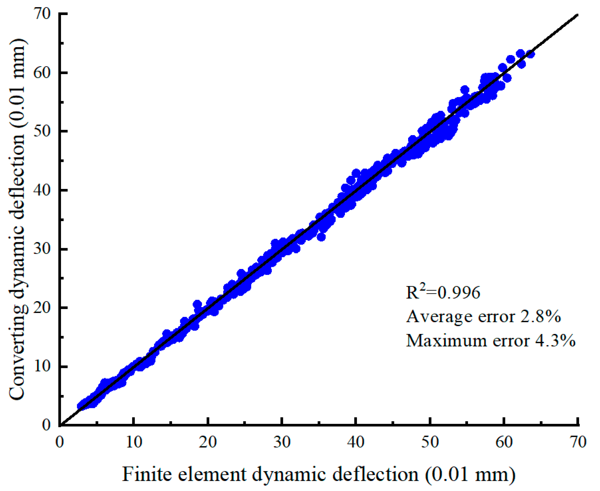
To assess the reliability of the dynamic deflection basin dataset, 50 pavement structure combinations were randomly selected, and their FWD deflection basins were calculated using the three-dimensional dynamic finite element method [26]. A total of 450 pairs of transformed dynamic deflection data and finite element-calculated deflection data were compared, as shown in Figure 2. The comparison reveals a high degree of consistency, with an average error of 2.8% and a maximum error of 4.3%. Based on these results, it can be concluded that the FWD dynamic deflection basin dataset established in this study is both accurate and comprehensive, effectively covering the range of pavement structures considered. As such, it is well-suited for use as a training dataset for the subsequent neural network model development.

2.2. BP Neural Network Model

A backpropagation (BP) neural network is a multilayer feedforward neural network trained using the backpropagation algorithm, which propagates the error between the model output and the target backward through the network. The BP deep learning model for back-calculating the moduli of pavement structural layers is shown in Figure 3.
The BP model training was carried out using the PyTorch framework. Key environment parameters for the training code are summarized in Table 5. We first preprocessed the dataset. In the labels, the surface-layer modulus is typically much larger than the subgrade modulus. To prevent scale disparities among multiple outputs—where large-magnitude targets could dominate the loss and induce gradient imbalance—and to enable clearer interlayer comparisons, we applied layer-wise scaling to the labels, bringing the surface and base layers to the same order of magnitude as the subgrade (e.g., with a subgrade range of 80–420 MPa and an asphalt range of 5000–14,500 MPa, the asphalt modulus is scaled by 1/100; for a rubblized layer range of 800–4200 MPa, it is scaled by 1/10). Feature variables were then nondimensionalized to ensure comparability and appropriate weighting across indicators with different units or scales, followed by normalization. To mitigate overfitting, the dataset was split into training and validation sets at a 7:3 ratio, and dropout layers were added to the network. The rectified linear unit (ReLU) activation was used to help prevent gradient explosion in deeper architectures, and the Adam optimizer was adopted to improve training efficiency and stability. Hyperparameters were tuned with Optuna; its adaptive Tree-structured Parzen Estimator (TPE) sampling is more computationally efficient and typically converges faster than grid or random search under limited trial budgets. Considering both computational resources and time, we selected representative hyperparameter configurations for evaluation, with search ranges and results reported in Table 6. The final optimized BP model comprised three hidden layers with 512 neurons each, a per-layer dropout rate of 0.1, a learning rate of 1 × 10⁻⁴, and a batch size of 1024.

2.3. Development of a Genetic Algorithm for Optimizing the BP

Genetic algorithm (GA) is a population-based global optimization method inspired by natural selection and genetic inheritance. Prior studies have shown that GA can facilitate the identification of favorable initial weights and biases for BP neural networks [18,19]. In this study, we design a GA to initialize the BP network used for modulus back-calculation; the GA-selected solution is subsequently refined via gradient-based training. Each encodes the complete set of BP parameters (weights and thresholds) in real-valued form, constrained to [−0.01, 0.01] so that initial activations lie in a stable, near-linear regime. Model quality is assessed by a fitness function that aggregates RMSE, MAE, and MAPE through their Euclidean norm, with fitness defined to be inversely related to this norm (i.e., lower error implies higher fitness). Each individual is trained for 50 epochs and evaluated on a fixed validation set. Selection is performed using tournament selection (k = 5), and crossover, together with mutation, is employed to balance global exploration and local exploitation. Following common GA practice, the crossover rate is restricted to [0.6, 0.9] and the mutation rate to [0.01, 0.1]. Implementation details are summarized in Table 7. Because a single fitness evaluation requires training a BP model to completion, we set the population size to 24 and the number of generations to 10 to balance computational cost and accuracy. The best individual returned by the GA is then used to initialize the BP network.

2.4. CNN Model

Convolutional neural networks (CNNs) are widely used due to their powerful ability to process features in two-dimensional data, such as images and videos [32]. The principles of feature extraction used by CNN for one-dimensional data are analogous to those for two-dimensional data. The predictive performance of CNN for one-dimensional data is comparable to that for two-dimensional data, as evidenced by their analysis [33]. This suggests that the powerful feature processing capabilities of convolutional and pooling layers can be equally applied to modulus back-calculation. Previous studies have also employed convolutional layers for feature extraction [14].
This paper employs a 1D-CNN as a feature extractor for the one-dimensional spatial sequence of input data (FWD dynamic deflection and layer thickness, totaling 11 dimensions). A small convolutional kernel (kernel = 3, stride = 1, padding = 1) is used to capture the continuity and overall configuration of adjacent deflection values through locality and translation invariance, while ensuring that the output aligns with the input length. This design enhances resilience to minor sampling deviations and noise. ReLU is applied to introduce nonlinearity after convolution, while max pooling (k = 2, s = 2) performs downsampling to aggregate multi-scale information and reduce computational load. This dimensionality reduction enables the CNN to learn global characteristics of deflection basins across modulus variations from local features. Consequently, distinctive traits of each deflection are preserved while significantly reducing the input dimensions to the fully connected layer. The flattening and fully connected layers perform feature integration and regression, with Dropout layers added to prevent overfitting. The model employs channel expansion by doubling the number of convolutional kernels per layer to enhance expressiveness. Shallow layers capture basic patterns, such as elastic deformation in deflection basins, while deeper layers identify more complex variations, such as distinctions between similar basins with different structural configurations or the impact of individual structural layer changes on deflection basins. The convolutional layers are limited to a maximum of three due to computational constraints. The remaining hyperparameters were optimized through an Optuna search. The proposed parameter ranges and results for optimization are shown in Table 8.
Compared to ANN, CNN significantly reduces the number of parameters through weight sharing. The use of 1D-CNN to convolve and pool the layered elastic responses of the FWD deflection basin effectively captures both local and global physical patterns associated with the layered elasticity between the deflection basin and modulus. This makes it well-suited for modulus back-calculation in three-layer pavement structures. This paper proposes a CNN specifically designed for pavement modulus back-calculation, leveraging these advantages. The model framework, data preprocessing, and activation functions are consistent with those of backpropagation (BP) neural networks. The final optimized hyperparameter combination yielded a CNN model comprising three convolutional layers, three pooling layers, and three fully connected layers. Each hidden layer contains 1024 neurons, with a dropout rate of 0.2, a learning rate of 2.37 × 10⁻⁴, and a training batch size of 128. The CNN deep learning model for pavement structure modulus back-calculation is shown in Figure 4.

3. Results and Discussion

3.1. Performance Analysis of the Single Model

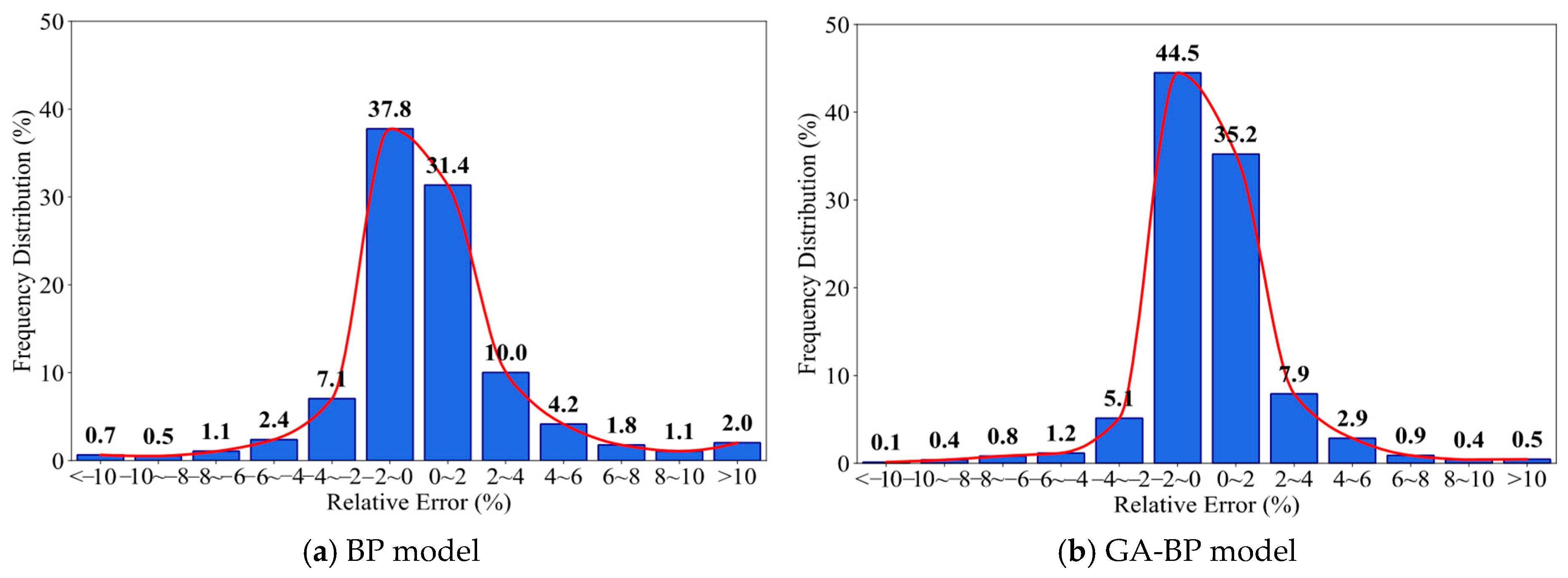
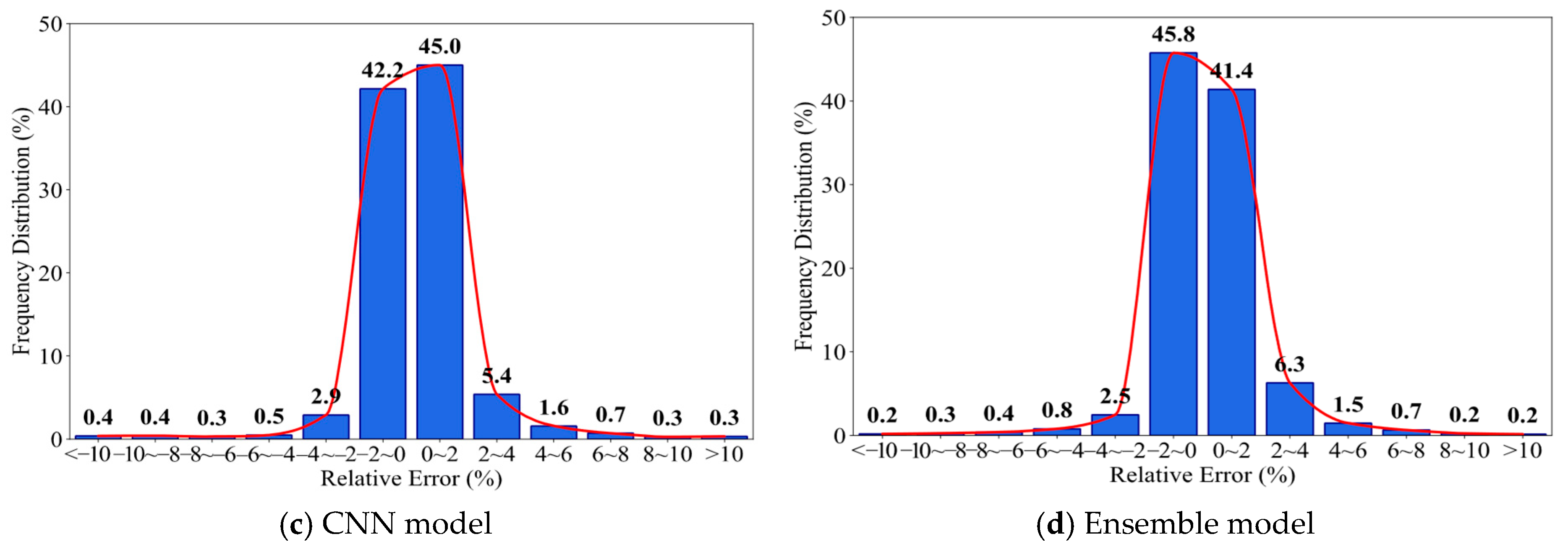
Using smaller validation datasets has been shown to lower both computational costs and time, while also providing valuable insights into how well the models perform [34]. According to the methodology outlined in Section 2.1, and ensuring coverage similar to that of randomly generated datasets, a FWD deflection validation dataset with 3600 pavement structure schemes was used. Various evaluation metrics were employed to thoroughly assess the overall and maximum error structures of the models, including RMSE, MAE, MAPE, Coefficient of Determination(R2), Mean Relative Error, and Maximum Relative Error. The evaluation parameters and error metrics are shown in Table 9, Table 10 and Table 11. The relative error distribution curves for different deep learning models on the validation dataset are displayed in Figure 5.
As shown in Table 9, the BP, GA-BP, and CNN models exhibit average relative errors of less than 5% in predicting the surface layer, base layer, and foundation moduli, with determination coefficients (R2) exceeding 0.98. These three modulus back-calculation models show significant improvement in performance compared to the ResRNN-W&D hybrid neural network model developed by Han et al. [15] (R2 = 0.70) and the LSTM model proposed by Al-Qaili et al. [17] (R2 = 0.93). This suggests that big data and deep learning models offer superior predictive accuracy and stability compared to neural network models trained on smaller datasets.
Further evaluation of model performance across structural layers reveals that the average error for subgrade modulus is consistently lower in all models compared to other layers, while the asphalt overlay modulus exhibits the highest average error. Given the influence of FWD data, this discrepancy is likely due to the reduced number of parameters reflecting asphalt modulus compared to the other two layers. Specifically, the subgrade modulus is influenced by both overall and distal tail deflection from FWD, while the asphalt layer modulus is jointly controlled by central deflection and thickness. The high prediction errors for the asphalt overlay layer primarily occur in extreme structural combinations, such as a 3 cm thickness with a modulus of 5000 megapascals. These structures account for most of the high-error cases, representing the main cause of the lower accuracy for the asphalt overlay layer. The modulus of such structural layers significantly influences central deflection but has a negligible effect on overall deflection. During the fitting process, deep learning models tend to align with broader data patterns rather than overfitting to individual data points, which further contributes to high errors in asphalt layer predictions.
We transitioned from analyzing common model characteristics to examining model differences. The initial values were used as the control variable to compare the GA-BP and BP models, with all other parameters held constant. The evaluated parameters and prediction error distributions of the GA-optimized GA-BP model demonstrate superiority over the BP model, supporting the hypothesis that GA can significantly enhance the prediction accuracy of BP neural networks within deep learning frameworks. This is further substantiated by the error distributions shown in Table 10 and Figure 5a,b.
The deep BP neural network has been shown to achieve theoretically optimal accuracy within a certain parameter range, with a relatively small gap in prediction accuracy compared to the CNN model, through the combined optimization of initial values and hyperparameters. The CNN model exhibits a lower mean error across all structural layers compared to the GA-BP model. This is likely due to CNN’s ability to effectively capture local correlations in deflection basin data through convolutional feature extraction, enabling it to extract more information from the same FWD data for modeling. However, the maximum errors of the CNN models exceed those of the GA-BP model, indicating residual instability risks. A thorough examination of Figure 5b,c, along with the evaluation metrics, confirms that CNN models demonstrate superior accuracy compared to GA-BP models, with both surpassing the performance of standard BP models. This finding suggests that, in the context of big data training, the extraction of dynamic deflection basin shape features by convolutional layers allows modulus back-calculation models to achieve overall prediction accuracy superior to that of BP-based models.
A combination of Figure 5 and Table 10 reveals that the relative errors in the back-calculation results from the trained prediction models are predominantly below 2%. However, the maximum relative error for individual models remains substantial. Notably, even the most proficient CNN model demonstrates a maximum relative error of up to 25.9%. This indicates that, despite the overall superior performance of the model, significant discrepancies persist between the predicted and actual modulus values in specific back-calculation scenarios. To apply the model more effectively in practical engineering, it is crucial to minimize the maximum error as much as possible to improve the model’s reliability in these specific scenarios.
As shown in Table 11, the maximum relative errors for both BP and GA-BP models occurred in the asphalt overlay layer. The corresponding thickness and modulus combinations were as follows: the thinnest surface layer with low modulus, and the thickest base layer with high modulus, or the thinnest base layer with low modulus. This finding indicates that the thicknesses of the surface and base layers significantly impact the accuracy of modulus back-calculation, a conclusion consistent with the results reported by Ghanizadeh et al. [35]. In contrast, the CNN model exhibits its maximum error at the subgrade level, where the thickness and modulus are neither at the upper nor lower extremes of the range. Moreover, under these conditions, the errors for the surface course and crushed stone layer also exceed 17.5%, which is substantially higher than the maximum error permitted by GA-BP (7.2%). This suggests that when the surface layer has a minimal contribution to the deflection basin, BP and GA-BP models are more prone to prediction instability near the training distribution boundary, resulting in significant errors. While CNNs demonstrate greater overall stability by learning global deflection basin characteristics based on local features, they may still produce significant errors in scenarios where the modulus-deflection correlation is weak. This finding suggests that the observed variation in prediction errors for pavement structural modulus between CNN and GA-BP is due to the distinct feature extraction methods employed by these models. Errors of this nature lead to overestimation when predicting low moduli, which in turn causes an underestimation of tensile and shear strains at the base of the surface layer in practical engineering applications. This has been shown to reduce the fatigue resistance of the surface structure and increase the risk of premature cracking. In contrast, when predicting high moduli, the errors are smaller, potentially resulting in excessive maintenance and higher costs. Therefore, considering the complementary nature of different neural network models in their back-calculation errors for pavement structural modulus, a computational approach based on model fusion back-calculation is a viable option. This approach has been shown to be effective in reducing the likelihood of significant errors while maintaining the overall back-calculation accuracy of the model.
In addition to CNN, experiments were conducted with RNN and LSTM architectures, which are theoretically well-suited for sequence modeling. However, in the course of our own experimental investigations, these models failed to attain satisfactory convergence performance. This outcome does not necessarily indicate that RNN or LSTM is ill-suited for modulus back-calculation; it may be attributable to the synthetic nature of the training dataset, wherein each FWD deflection basin signifies an autonomous structural response devoid of explicit temporal dependencies or long-term evolution patterns. The fundamental design of RNN and LSTM algorithms aims to capture temporal correlations and sequence dependencies. However, these characteristics are not prominent in the current dataset. Conversely, CNNs leverage local spatial feature extraction to learn characteristics related to the shape of deflection basins, which are directly correlated with variations in layer modulus.

3.2. Analysis of the CNN and GA-BP Ensemble Model

Given the strong predictive accuracy of both CNN and GA-BP and their complementary error patterns across pavement layers, we adopt a linear ensemble of their outputs (Figure 6). This leverages the models’ distinct nonlinear mapping mechanisms, yielding complementary strengths in modulus back-calculation. When no single sub-model is uniformly superior, equal-weight averaging is widely regarded as a robust default [36]. To select weights, we vary the CNN weight and evaluate ensemble variants using the Euclidean norm of RMSE, MAE, MAPE, alongside R2 (Figure 7). As the CNN weight approaches 0.5, R2 increases while the error norm decreases, indicating a near-optimal balance at equal weights; accordingly, we set β1 = β2 = 0.5. This equal-weight ensemble approach not only theoretically ensures robustness when the accuracies of the sub-models are close but also avoids additional tuning costs in engineering applications, making it more practical. However, it is important to note that, while the ensemble model enhances the prediction performance of the back-calculation model, the overall effect may be limited if the individual sub-models exhibit large prediction errors.
The ensemble model was used to back-calculate the pavement structural modulus on the validation dataset, with results in Table 9 and Table 10. The relative error distribution of the ensemble model on this dataset is shown in Figure 5d. The deep learning evaluation metrics (R2, MAE, RMSE, MAPE) have further improved. Compared with the best single model (CNN), the fused model attains higher R2 for the surface/rubblized/subgrade layers—0.995/0.999/0.996—and achieves the lowest (or joint-lowest) MAE and RMSE across layers. Maximum relative errors drop markedly: surface 20.3% → 17.3% (−14.8%), rubblized 18.1% → 15.3% (−15.5%), and subgrade 25.9% → 14.9% (−42.5%). The share of samples with <5% error rises from 96.7% to 97.3%, while those >10% fall from 0.4% to 0.3%. The only minor exception is MAPE for the rubblized layer, where the fused value (0.908%) is slightly higher than CNN (0.871%)—an acceptable trade-off given the overall gains. The quality range of the error histogram after ensemble integration is nearly identical to that of the CNN model. Consequently, the ensemble model’s back-calculation of the asphalt pavement structural modulus has a less than 3% chance of exceeding a 5% relative error, with the maximum relative error staying below 17.3%. The model demonstrates satisfactory accuracy, stability, and generalization, meeting the requirements for practical engineering applications.

3.3. Ensemble Model Engineering Validation

The research verification data consists of deflection basin data obtained from the FWD deflection tests conducted on the engineering section K3317 + 000 to K3317 + 875. After correcting the measured deflection basin data for temperature and humidity to standard conditions (20 °C, 50% relative humidity), and with the structural layer thickness already known, the modulus of each structural layer can be back-calculated using the deflection basin test data. Since on-site deflection measurements can be influenced by the traffic on the opposite lane, the “3σ principle” was applied to remove any outlier deflection basin data, improving the reliability of the data. Subsequently, the remaining 30 deflection basin data points were statistically analyzed, and the results are shown in Table 12 [25].
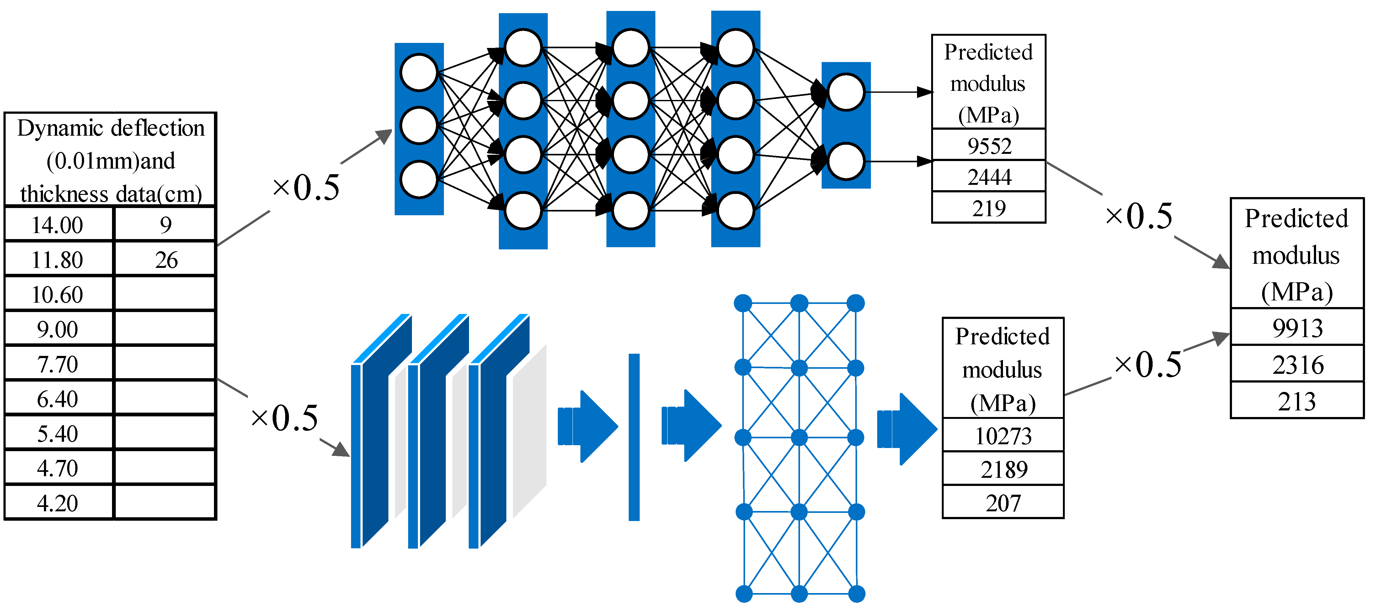
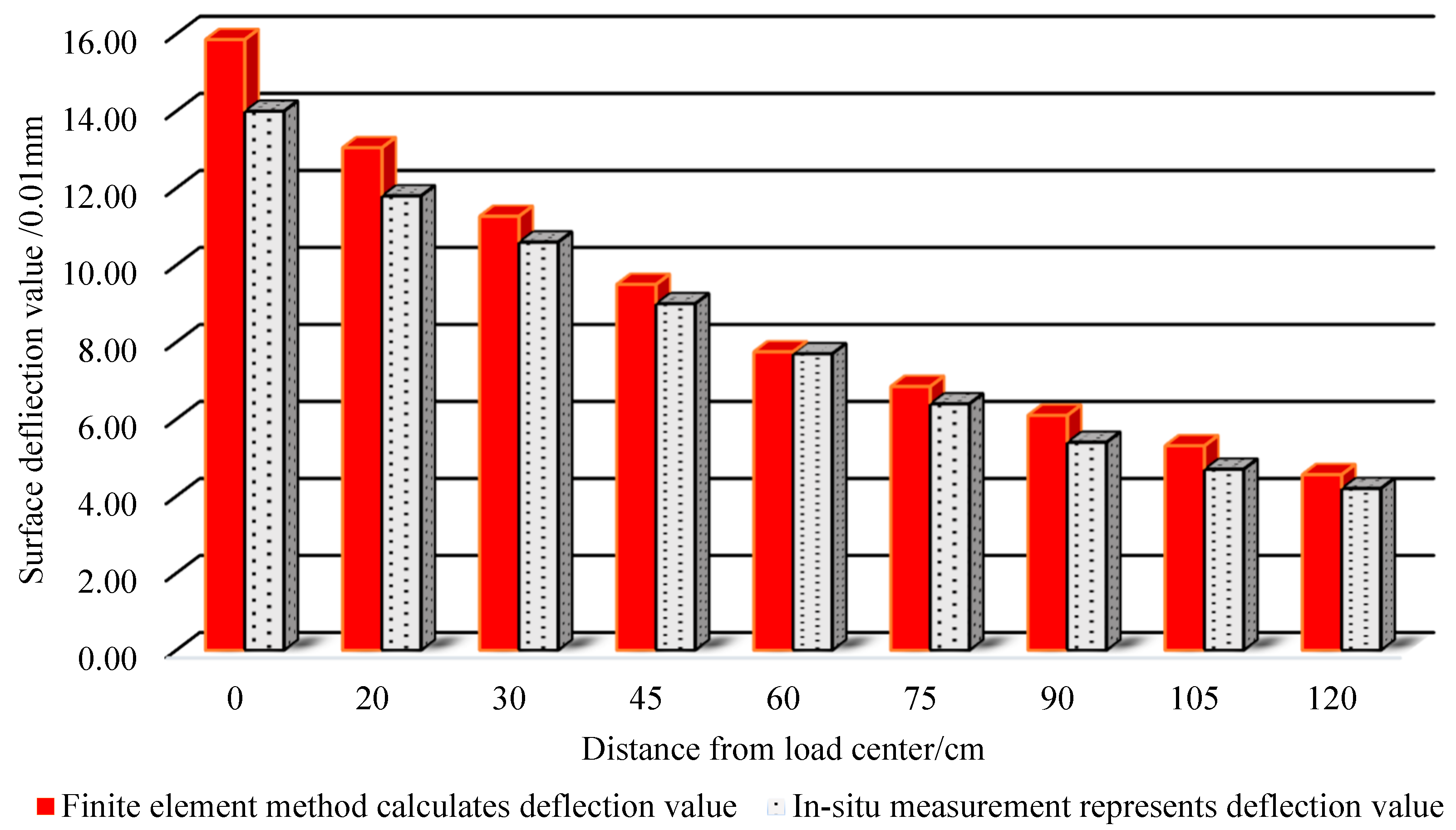
Using the pavement structure and simplified models from Table 1 and Table 2, along with the representative deflection basin values from Table 12, an ensemble model combining CNN and GA-BP was used to back-calculate the dynamic moduli of the asphalt overlay, rubblized layer, and subgrade. As shown in Figure 8, the back-calculated dynamic moduli were 9913 MPa, 2316 MPa, and 213 MPa, respectively. Based on the back-calculated dynamic moduli and the three-layer pavement structural model presented in Table 2, the three-dimensional dynamic finite element method [26] was employed to compute the FWD deflection basin data at the pavement surface, as shown in Table 13. A comparison between the calculated deflection basin and the measured representative deflection basin values is shown in Figure 9.
As shown in the comparative analysis of Table 12 and Table 13, and Figure 9, the deflection basin values calculated using the back-calculated moduli are generally higher than the measured values, with a root mean square error (RMSE) of 0.88%, indicating only minor deviations. This result demonstrates that the ensemble model combining CNN and GA-BP achieves high reliability and accuracy in back-calculating the dynamic moduli of asphalt pavement structural layers, meeting the precision requirements for engineering applications. Furthermore, the analysis reveals that the dynamic modulus of the resonance crushed stone layer significantly exceeds the modulus range of conventional graded aggregate bases used in highway engineering (250–700 MPa). This suggests that after the old cement concrete pavement is resonance-crushed, the tightly interlocked fragments form a layer with slab-like characteristics and significantly enhanced load-bearing capacity.

4. Summary and Conclusions

This study provides an accurate and reliable solution for back-calculating the structural modulus of crushed asphalt overlay on old cement concrete pavements. Based on a dynamic deflection dataset derived from a simplified three-layer structure (“asphalt layer–rubblized layer–subgrade”) of the reference project, BP, GA-BP, and CNN deep learning models were developed and analyzed for their performance in predicting the dynamic modulus of asphalt pavement structural layers. Subsequently, an integrated modulus back-calculation model for fractured old cement concrete asphalt pavement was proposed, leading to several important conclusions.
  • Based on model-evaluation metrics and error-distribution analyses, all three models (BP, GA-BP, and CNN) trained on the large-scale FWD dynamic-deflection dataset exhibit high predictive performance (R2 > 0.981). The CNN back-calculation model attains lower mean errors than GA-BP, and both models outperform the plain BP model (R2 > 0.993 for CNN/GA-BP), indicating greater application potential for CNN in modulus back-calculation of asphalt overlays on rubblized concrete pavements.
  • On the validation set, CNN and GA-BP display complementary maxima across layers and extreme parameter combinations. An equal-weight linear ensemble, motivated by this complementarity, substantially reduces tail risk: the maximum relative error drops from 25.9% (CNN) to 17.3%, and the share of cases with <5% error increases from 96.7% to 97.3%. Mean-based metrics (MAE, RMSE) and R2 also improve. These results indicate that the ensemble lowers worst-case errors while enhancing overall stability and accuracy.
  • External consistency checks and closed-loop field-segment validation using 3D dynamic finite-element analysis show strong agreement among simulation, back-calculation, and field measurements: the average dataset error is ≈2.8% (maximum ≈ 4.3%), and the RMSE for representative field deflection basins is ≈0.88%. Collectively, these findings demonstrate that the CNN + GA-BP ensemble model delivers high accuracy, reliability, and generalization for predicting dynamic moduli of pavement structural layers on rubblized concrete bases.
The proposed hybrid model integrates GA–BP and CNN to improve the stability and accuracy of modulus back-calculation. Multi-model ensembling reduces single-model randomness and variability while retaining ANN-level speed for high-throughput processing. It supports large-scale back-calculation and extends coverage across a wide range of pavement configurations. These properties make it suitable for intelligent pavement monitoring and maintenance planning. (1) Intelligent monitoring: Batch inversion produces near-real-time modulus maps for anomaly zoning and early-deterioration alerts. (2) Maintenance planning: Modulus and uncertainty assessments guide intervention priorities and optimize annual programs. Decision support: Integration with network-level FWD data and asset management systems enables the creation of budget scenarios and resource allocation. This work focuses on an end-to-end deep model. A broader benchmarking of classical ensembles (e.g., CatBoost with tailored feature engineering) is left for future work.

Limitations and Future Work

Although the generated database is comprehensive—covering a wide range of pavement structures and parameter combinations—several limitations remain. These mainly arise from discrepancies between finite-element deflection data and in situ measurements, as well as between standardized deflection data and real-world operating conditions. It is also important to investigate how geographical and climatic variability influences in-service modulus values. Looking ahead, we will develop higher-precision models capable of handling more complex pavement-structure data and strengthen procedures for standardizing/correcting dynamic deflection data across different environments. Because this work focuses on an end-to-end deep model, a broader, carefully tuned benchmarking of classical ensemble methods (e.g., XGBoost with tailored feature engineering) falls outside the present scope and is left for future work. These advances will be validated on multi-site, real-world datasets spanning diverse pavement types and complex weather conditions to further assess the predictive performance of deep learning for pavement modulus estimation.

Author Contributions

Conceptualization and methodology, P.P.; software and validation, P.P.; data curation and resources, Q.L.; writing—original draft, P.P.; writing—review and editing, Q.L. and P.P. All authors have read and agreed to the published version of the manuscript.

Funding

This research received no external funding.

Institutional Review Board Statement

Not applicable.

Informed Consent Statement

Not applicable.

Data Availability Statement

The original contributions presented in this study are included in the article. Further inquiries can be directed to the corresponding author.

Conflicts of Interest

No potential conflict of interest was reported by the authors.

References

  1. Papavasiliou, V.; Loizos, A. Field performance and fatigue characteristics of recycled pavement materials treated with foamed asphalt. Constr. Build. Mater. 2013, 48, 677–684. [Google Scholar] [CrossRef]
  2. El-Raof, H.S.A.; El-Hakim, R.T.A.; El-Badawy, S.M.; Afify, H.A. Simplified closed-form procedure for network-level determination of pavement layer moduli from falling weight deflectometer data. J. Transp. Eng. Part B Pavements 2018, 144, 04018052. [Google Scholar] [CrossRef]
  3. Zeiada, W.; Dabous, S.A.; Hamad, K.; Al-Ruzouq, R.; Khalil, M.A. Machine learning for pavement performance modelling in warm climate regions. Arab. J. Sci. Eng. 2020, 45, 4091–4109. [Google Scholar] [CrossRef]
  4. Zaman, M.; Solanki, P.; Ebrahimi, A.; White, L. Neural network modeling of resilient modulus using routine subgrade soil properties. Int. J. Geomech. 2010, 10, 1–12. [Google Scholar] [CrossRef]
  5. You, L.; Yan, K.; Liu, N. Assessing artificial neural network performance for predicting interlayer conditions and layer modulus of multi-layered flexible pavement. Front. Struct. Civ. Eng. 2020, 14, 487–500. [Google Scholar] [CrossRef]
  6. Tarefder, R.A.; Ahsan, S.; Ahmed, M.U. Neural network–based thickness determination model to improve back-calculation of layer moduli without coring. Int. J. Geomech. 2015, 15, 04014058. [Google Scholar] [CrossRef]
  7. Elbagalati, O.; Elseifi, M.A.; Gaspard, K.; Zhang, Z. Development of an artificial neural network model to predict subgrade resilient modulus from continuous deflection testing. Can. J. Civ. Eng. 2017, 44, 700–706. [Google Scholar] [CrossRef]
  8. Ceylan, H.; Schwartz, C.W.; Kim, S.; Gopalakrishnan, K. Accuracy of predictive models for dynamic modulus of hot-mix asphalt. J. Mater. Civ. Eng. 2009, 21, 286–293. [Google Scholar] [CrossRef]
  9. Sharma, S.; Das, A. Back-calculation of pavement layer moduli from falling weight deflectometer data using an artificial neural network. Can. J. Civ. Eng. 2008, 35, 57–66. [Google Scholar] [CrossRef]
  10. Wang, H.; Li, M.; Szary, P.; Hu, X. Structural assessment of asphalt pavement condition using backcalculated modulus and field data. Constr. Build. Mater. 2019, 211, 943–951. [Google Scholar] [CrossRef]
  11. Ghasemi, P.; Aslani, M.; Rollins, D.K.; Williams, R.C. Principal component neural networks for modeling, prediction, and optimization of hot-mix asphalt dynamic modulus. Infrastructures 2019, 4, 53. [Google Scholar] [CrossRef]
  12. Zhang, C.; Shen, S.; Huang, H.; Yu, S. In situ dynamic modulus prediction for asphalt pavement combining machine learning algorithm and sensing technology. IEEE Trans. Intell. Transp. Syst. 2024, 25, 8695–8704. [Google Scholar] [CrossRef]
  13. Fan, J.; Ma, T.; Zhu, J.; Zhu, Y.; Zhang, Y. Characteristics of high-speed deflection basin and structural-parameter back-calculation of asphalt pavement with different structural states. Constr. Build. Mater. 2022, 341, 127869. [Google Scholar] [CrossRef]
  14. Moussa, G.S.; Owais, M. Modeling hot-mix asphalt dynamic modulus using deep residual neural networks: Parametric and sensitivity analysis study. Constr. Build. Mater. 2021, 294, 123589. [Google Scholar] [CrossRef]
  15. Han, C.; Ma, T.; Chen, S.; Fan, J. Application of a hybrid neural network structure for FWD back-calculation based on LTPP database. Int. J. Pavement Eng. 2022, 23, 3099–3112. [Google Scholar] [CrossRef]
  16. Al-Qaili, A.H.; Al-Mansour, A.I.; Al-Solieman, H.; Alsharabi, K. RNN-based pavement moduli prediction for flexible pavement design enhancement. Case Stud. Constr. Mater. 2024, 20, e02811. [Google Scholar] [CrossRef]
  17. Al-Qaili, A.H.; Al-Mansour, A.I.; Al-Solieman, H.; Abduh, Z.; Lee, S.M. Adaptation of an alternative neural network instead of an ANN for back-calculating pavement layer moduli. Constr. Build. Mater. 2024, 438, 137281. [Google Scholar] [CrossRef]
  18. Ghorbani, B.; Arulrajah, A.; Narsilio, G.; Horpibulsuk, S.; Bo, M.W. Development of genetically based models for predicting the resilient modulus of cohesive pavement subgrade soils. Soils Found. 2020, 60, 398–412. [Google Scholar] [CrossRef]
  19. Li, M.; Wang, H. Development of ANN–GA program for back-calculation of pavement moduli under FWD testing with viscoelastic and nonlinear parameters. Int. J. Pavement Eng. 2019, 20, 490–498. [Google Scholar] [CrossRef]
  20. Li, M.; Wang, H. Prediction of asphalt pavement responses from FWD surface deflections using soft computing methods. J. Transp. Eng. Part B Pavements 2018, 144, 04018014. [Google Scholar] [CrossRef]
  21. Fan, H.; Zhang, J.; Zheng, J. Back-calculation of nonlinear properties of subgrade using a new in situ nondestructive testing approach based on loading sequence. Int. J. Geomech. 2024, 24, 04024235. [Google Scholar] [CrossRef]
  22. Li, M.; Dai, Q.; Su, P.; You, Z.; Ma, Y. Surface layer modulus prediction of asphalt pavement based on LTPP database and machine learning for mechanistic–empirical rehabilitation design applications. Constr. Build. Mater. 2022, 344, 128303. [Google Scholar] [CrossRef]
  23. Svilar, M.; Peško, I.; Šešlija, M. Model for estimating the modulus of elasticity of asphalt layers using machine learning. Appl. Sci. 2022, 12, 10536. [Google Scholar] [CrossRef]
  24. Wang, Y.; Zhao, Y.; Sun, Q.; Wang, R. Intelligent back-calculation of elastic modulus for asphalt pavement structures with bedrock using a stacking ensemble learning model. Constr. Build. Mater. 2025, 491, 142704. [Google Scholar] [CrossRef]
  25. Liu, Z.; Liu, D. Dynamic modulus analysis of the resonantly rubblized layer of old cement concrete slab based on BP neural network and deep learning model. Highway 2024, 69, 44–51. (In Chinese) [Google Scholar]
  26. Li, Q.; Chen, Z. Numerical analysis and conversion of dynamic and static deflection of asphalt pavement under FWD loading. Constr. Build. Mater. 2023, 367, 129513. [Google Scholar] [CrossRef]
  27. Tarefder, R.A.; Ahmed, M.U. Modeling of the FWD deflection basin to evaluate airport pavements. Int. J. Geomech. 2014, 14, 205–213. [Google Scholar] [CrossRef]
  28. JTG D50-2017; Specifications for Design of Highway Asphalt Pavement. China Standard Press: Beijing, China, 2017.
  29. Ling, C.; David, E.; Siddharthan, R. Comparison of dynamic and static back-calculation moduli for three-layer pavements. Transp. Res. Rec. 1991, 1293, 86–92. [Google Scholar]
  30. Wu, C.; Wang, H.; Zhao, J.; Jiang, X.; Qiu, Y. Asphalt pavement modulus back-calculation using surface deflections under moving loads. Comput.-Aided Civ. Infrastruct. Eng. 2020, 35, 1246–1260. [Google Scholar] [CrossRef]
  31. Gandomi, A.H.; Yang, X.S.; Talatahari, S.; Alavi, A.H. Metaheuristic algorithms. In Metaheuristic Applications in Structures and Infrastructures; Elsevier: Amsterdam, The Netherlands, 2013; pp. 1–24. [Google Scholar]
  32. Gu, J.; Wang, Z.; Kuen, J.; Ma, L.; Shahroudy, A.; Shuai, B.; Liu, T.; Wang, X.; Wang, G.; Cai, J.; et al. Recent advances in convolutional neural networks. Pattern Recognit. 2018, 77, 354–377. [Google Scholar] [CrossRef]
  33. Ige, A.O.; Sibiya, M. State-of-the-art in 1D convolutional neural networks: A survey. IEEE Access 2024, 12, 144082–144105. [Google Scholar] [CrossRef]
  34. Almufti, S.M.; Shaban, A.A.; Ali, Z.A.; Ali, R.I.; Fuente, J.D. Overview of metaheuristic algorithms. Polaris Glob. J. Sch. Res. Trends 2023, 2, 10–32. [Google Scholar] [CrossRef]
  35. Ghanizadeh, A.R.; Heidarabadizadeh, N.; Jalali, F. Artificial neural network back-calculation of flexible pavements with sensitivity analysis using Garson’s and connection weights algorithms. Innov. Infrastruct. Solut. 2020, 5, 63. [Google Scholar] [CrossRef]
  36. Wang, X.; Hyndman, R.J.; Li, F.; Kang, Y. Forecast combinations: An over 50-year review. Int. J. Forecast. 2023, 39, 1518–1547. [Google Scholar] [CrossRef]
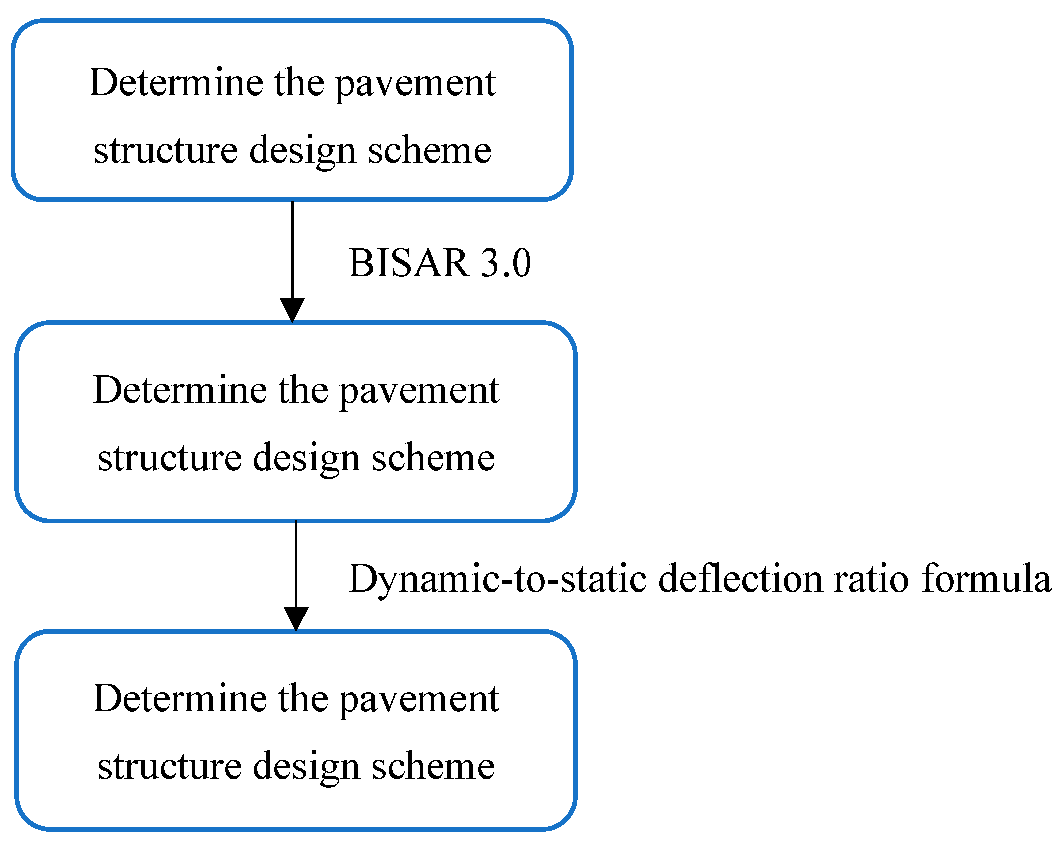
Figure 1. Procedural diagram for generating a dynamic deflection database.
Applsci 15 11115 g001
Figure 2. Comparison of finite element dynamic deflection and dynamic-static ratio converted deflection.
Applsci 15 11115 g002
Figure 3. BP neural network deep learning model for back-calculation of pavement structural layer moduli.
Applsci 15 11115 g003
Figure 4. CNN deep learning model for back-calculation of pavement structural layer moduli.
Applsci 15 11115 g004
Figure 5. Histogram of overall error distribution for modulus back-calculation models on the validation set.
Applsci 15 11115 g005aApplsci 15 11115 g005b
Figure 6. Model ensemble approach.
Applsci 15 11115 g006
Figure 7. Variation in evaluation metrics for the ensemble model under different weight combinations.
Applsci 15 11115 g007
Figure 8. Flowchart of the ensemble model for modulus back-calculation.
Applsci 15 11115 g008
Figure 9. Comparison of the finite element calculated deflection basin and the representative in situ FWD measured deflection basin.
Applsci 15 11115 g009
Table 1. Structural analysis parameters for resonantly rubblized old cement concrete pavement with asphalt overlay.
No.Pavement Structural LayersThickness (cm)Poisson’s RatioDensity (kg·m−3)
1AC-16 medium-graded asphalt concrete surface layer40.252450
2AC-20 medium-graded asphalt concrete binder layer50.252450
3Resonance-crushed cement concrete layer260.302500
4Old cement-stabilized crushed stone base layer180.302400
5Graded crushed stone subbase layer180.352250
6Subgrade soil layer-0.402100
Table 2. Simplified structural model and analysis parameters for modulus back-calculation.
Pavement Structural Layer DivisionThickness (cm)Poisson’s RatioDensity (kg·m3)
Asphalt overlay layer90.252450
Resonant-crushed stone layer260.302500
Old cement-stabilized crushed stone layer + Old graded crushed stone layer + Soil base.-0.352250
Table 3. Computational scheme for the dynamic deflection database of cement concrete rubblized asphalt pavement structure.
Pavement Structural LayerThicknessPoisson’s RatioModulus
Range (cm)Number of ValuesRange (MPa)Number of Values
Asphalt overlay layer3–2220 *0.255000–14,50020
Resonance-crushed stone layer18–40120.30800–420018 *
Subgrade--0.3580–42018
Note: The number of values refers to the quantity of randomly selected thickness and modulus values within their respective ranges. For example, “20 *” indicates that 20 thickness values were randomly selected from the range of 4 to 22 cm for the asphalt overlay layer, while “18 *” indicates that 18 modulus values were randomly selected from the range of 800 to 4200 MPa for the resonance-crushed stone layer.
Table 4. Sensor configuration of the integrated FWD deflection device.
Sensor PositionD1D2D3D4D5D6D7D8D9
Distance to load center (cm)0203045607590105120
Table 5. Summary of experimental environment.
Hardware and SoftwareModel and Version
GPUNvidia GeForce RTX 4060ti
CPU13th Gen Intel(R) Core(TM) i5-13400F
Operating systemWindows 11 professional
Pycharm2024.2.4 professional
Pytorch1.12.1
Python3.8.20
Scikit-lrean1.3.0
Matplotlib3.7.2
Numpy1.24.3
Pandas2.0.3
Tqdm4.66.5
Optuna4.0.0
Table 6. Hyperparameters of the BP model.
HyperparametersRangesResults
Number of hidden layers1, 2, 3, 4, 53
Number of hidden neurons64, 128, 256, 512, 1024512
Learning rate range0.001–0.000010.0001
Dropout rate0.1, 0.2, 0.30.1
Training batch size64, 128, 256, 512, 10241024
Table 7. Construction method of the genetic algorithm for optimizing the BP.
ModuleConstruction MethodsRelevant Formulas
Genetic encodingReal-number encoding-
Fitness evaluation- F = 1 n 1 R M S E 2 + M A E 2 + M A P E 2 100
Selection operatorTournament selection-
Crossover operatorArithmetic crossover C 1 i = 1 α P 1 i + α P 2 i C 2 i = α P 1 i + 1 α P 2 i
Mutation operatorUniform mutation C i = C i if   random ( ) p mutate random ( a i , b i ) if   random ( ) < p mutate
Parameter configurationAdaptive crossover rate p c = 0.8 f max f avg f avg f min + λ   if   f max f avg f avg f min + λ < 1 and   M 1 > M 2 p c 1 p c 1 p c 2 f f min f max f min   otherwise
Adaptive mutation rate p m = 0.1 f max f avg f avg f min + λ if f max f avg f avg f min + λ < 1   and   M 1 > M 2 p m 1 p m 1 p m 2 f f min f max f min otherwise
Population size l = x × m 1 + m 1 + m 1 × m 2 + m 2 + + m n + m n × s + s
The encoding range, the number of iterations, and the neural network iteration count are determined empirically.
Table 8. Hyperparameters of the CNN model.
HyperparametersRangesResults
Number of convolutional layers1, 2, 33
Number of hidden layers2, 3, 4, 53
Number of neurons64, 128, 256, 512, 10241024
Learning rate range0.001–0.000010.0002
Dropout rate0.1, 0.2, 0.30.2
Training batch size64, 128, 256, 512, 10241024
Table 9. Comparison of evaluation metrics for pavement layer modulus back-calculation models.
ModelPavement Structural LayersPavement Structure Scheme QuantityEvaluation ParameterRelative Error (%)
R2MAERMSEMAPEAverage ValueMaximum Value
BPAsphalt overlay layer36000.9813.3324.7473.7103.738.0
Resonance-crushed stone layer0.9964.4807.5201.9401.921.7
Subgrade0.9873.1615.7301.1961.221.9
GA-BPAsphalt overlay layer0.9931.8652.8372.0552.120.9
Resonance-crushed stone layer0.9983.0374.9021.3661.417.6
Subgrade0.9952.2153.5840.8400.813.4
CNNAsphalt overlay layer0.9941.7172.7631.8161.820.3
Resonance-crushed stone layer0.9982.2314.7310.8710.918.1
Subgrade0.9941.5903.7620.6140.625.9
Ensemble modelAsphalt overlay layer0.9951.5222.3661.6421.617.3
Resonance-crushed stone layer0.9992.1484.0260.9080.913.1
Subgrade0.9961.5563.1900.5990.614.9
Table 10. Statistical distribution of relative back-calculation error (%) by model.
Pavement Structural LayersBP ModelGA-BP ModelCNN ModelEnsemble Model
<2%<5%<10%<2%<5%<10%<2%<5%<10%<2%<5%<10%
Asphalt overlay layer41.677.093.065.790.598.871.992.598.673.894.199.4
Resonance-crushed stone layer66.793.298.579.697.299.693.698.899.790.998.899.9
Subgrade85.996.399.393.898.699.896.098.899.596.698.999.7
Average value64.788.896.979.795.499.487.296.799.387.197.399.7
Table 11. Comparative analysis of the maximum relative error generated by different neural network modulus back-calculation models.
Pavement Structural LayersBP Maximum Relative Error Pavement StructureGA-BP Maximum Relative Error Pavement StructureCNN Maximum Relative Error Pavement Structure
Structural InformationBack-Calculation Modulus (MPa)Structural InformationBack-Calculation Modulus (MPa)Structural InformationBack-Calculation Modulus (MPa)
Thickness (cm)Modulus (MPa)BPGA-BPCNNThickness (cm)Modulus (MPa)BPGA-BPCNNThickness (cm)Modulus (MPa)BPGA-BPCNN
Asphalt overlay layer3500069015715598035000579660435698226920773474158189
Resonance-crushed stone layer40420039394150413118800801818794324200430042304939
Subgrade-350349347348-292289293291-274298294345
Table 12. Statistical analysis results of in situ FWD measured deflection basin data (0.01 mm).
Sensor PositionD1D2D3D4D5D6D7D8D9
Mean deflection 12.1010.209.007.606.505.404.604.003.60
The standard deviation of deflection1.781.561.501.321.140.930.800.630.55
Coefficient of variation0.150.150.170.170.180.170.170.160.15
Representative deflection14.0011.8010.609.007.706.405.404.704.20
Table 13. Surface dynamic deflection basin calculated by the three-dimensional dynamic finite element model (0.01 mm).
Sensor PositionD1D2D3D4D5D6D7D8D9RMSE of Measured Deflection (%)
Dynamic deflection15.8613.0511.279.507.756.856.15.314.560.88
Disclaimer/Publisher’s Note: The statements, opinions and data contained in all publications are solely those of the individual author(s) and contributor(s) and not of MDPI and/or the editor(s). MDPI and/or the editor(s) disclaim responsibility for any injury to people or property resulting from any ideas, methods, instructions or products referred to in the content.