Article

Sensor-Level Anomaly Detection in DC–DC Buck Converters with a Physics-Informed LSTM: DSP-Based Validation of Detection and a Simulation Study of CI-Guided Deception

1
Department of Electronic Engineering, Chosun University, Gwangju 61452, Republic of Korea
2
Department of Software, Paichai University, Daejeon 35345, Republic of Korea
3
Department of Automotive Engineering, Honam University, Gwangju 62399, Republic of Korea
*
Author to whom correspondence should be addressed.
Appl. Sci. 2025, 15(20), 11112; https://doi.org/10.3390/app152011112
Submission received: 7 September 2025 / Revised: 29 September 2025 / Accepted: 9 October 2025 / Published: 16 October 2025

Abstract

Digitally controlled DC–DC converters are vulnerable to sensor-side spoofing, motivating plant-level anomaly detection that respects the converter physics. We present a physics-informed LSTM (PI–LSTM) autoencoder for a 24→12 V buck converter. The model embeds discrete-time circuit equations as residual penalties and uses a fixed decision rule ( τ = μ + 3 σ , N = 3 consecutive samples). We study three voltage-sensing attacks (DC bias, fixed-sample delay, and narrowband noise) in MATLAB/Simulink. We then validate the detection path on a TMS320F28379 DSP. The detector attains F1 scores of 96.12%, 91.91%, and 97.50% for bias, delay, and noise (simulation); on hardware, it achieves 2.9–4.2 ms latency with an alarm-wise FPR of ≤1.2%. We also define a unified safety box for DC rail quality and regulation. In simulations, we evaluate a confusion index (CI) policy for safety-bounded performance adjustment. A operating point yields CI 0.25 while remaining within the safety limits. In hardware experiments without CI actuation, the V r , p p and IRR stayed within the limits, whereas the ±2% regulation window was occasionally exceeded under the delay attack (up to ≈2.8%). These results indicate that physics-informed detection is deployable on resource-constrained controllers with millisecond-scale latency and a low alarm-wise FPR, while the full hardware validation of CI-guided deception (safety-bounded performance adjustment) under the complete safety box is left to future work.

1. Introduction

1.1. Research Background

Modern power electronic systems are increasingly exposed to cyber-physical threats due to the pervasive use of digital controllers and communication networks [1,2]. DC–DC buck converters, as core building blocks in industrial supplies, EV chargers, and renewable interfaces, are natural targets for sensor-side spoofing [3,4]. Network-centric defenses alone are insufficient for such plant-level attacks because they do not provide real-time, physics-consistent anomaly detection at the converter I/O [5,6,7].

1.2. Limitations of Existing Research

Prior studies have emphasized protocol security or network intrusion detection, with comparatively less focus on sensor-level detection in power converters [8,9]. Converter-oriented detectors are often statistical/rule-based and struggle with subtle, dynamics-driven deviations in high-rate time series. Moreover, many approaches lack explicit physical constraints, clear decision rules, and hardware evidence of deployability under tight real-time budgets [10,11].

1.3. Related Work and Context

Prior efforts can be grouped into six strands: (i) model-/observer-based FDI (Kalman/EKF, unknown-input observers, parity space), (ii) rule/statistical change detection (CUSUM/GLR on residuals), (iii) classical ML (SVM, random forest, isolation forest), (iv) deep time-series autoencoders (CNN–LSTM/LSTM AEs), (v) physics-informed learning (constraints embedded in the loss), and (vi) CPS security for converters (sensor path anomalies and EMI/delay effects). Our approach sits at the intersection of (iv) and (v): a PI–LSTM with discrete-time circuit residuals aligned to fixed-step control, a fixed decision rule ( τ = μ + 3 σ , N = 3 ), and hardware validation of the detection latency/FPR under a unified safety box. The prior research landscape is summarized in Table 1.
Positioning. Relative to (i)–(iii), PI constraints reduce spurious alarms by disallowing reconstructions that violate the converter physics; relative to (iv), we enforce discrete-time residuals (not continuous PDEs), which matches embedded fixed-step deployment. The safety box (regulation, V r , pp , IRR) bridges detection and system metrics.
Classic references. Foundational FDI/CM and power electronics surveys include Isermann’s monograph on model-based and statistical fault diagnosis [12], the converter device reliability and condition monitoring review by Yang et al. [21], online capacitor monitoring in converters by Buiatti et al. [22], the comprehensive DC–DC monitoring framework by Givi et al. [13], and the focused review of fault diagnosis/tolerance for DC–DC converters by Geddam and Elangovan [14].

Classical Detectors (EKF/Fuzzy/CUSUM)

Prior converter-oriented detectors include (i) Kalman filter residual schemes (EKF/UKF) that threshold the innovation or its normalized energy; (ii) fuzzy/rule-based logic crafted from expert heuristics; and (iii) classical change detection (Shewhart, CUSUM/GLR). They are lightweight and interpretable but may be sensitive to model mismatch/drift and hand-tuned thresholds under nonstationary operating conditions. To contextualize our PI–LSTM, we later benchmark an EKF residual detector and a Shewhart detector under the same preprocessing conditions and decision rule ( τ = μ + 3 σ , N = 3 ).

1.4. Research Objectives and Contributions

We propose a physics-informed anomaly detector and a safety-aware response tailored to digitally controlled DC–DC converters. The unique contributions of this paper are as follows.
  • Discrete-time physics-informed LSTM (PI–LSTM) for converters. We embed the averaged buck dynamics as residual penalties on decoder trajectories, avoiding label leakage and aligning with fixed-step embedded control; the residual template is topology-agnostic via the replacement of the discrete-time update map [23].
  • Unified detection policy with DSP-grade deployment. A single detector covers DC bias, fixed-sample delay, and narrowband noise under a fixed decision rule ( τ = μ + 3 σ , N = 3 ). On a TMS320F28379, a distilled model ( n x = 4 , n h = 32 ) achieves 2.9–4.2 ms latency with an alarm-wise FPR of ≤1.2%.
  • Unified safety box coherently tied to response. We formalize a safety box for DC rail quality and regulation—time-domain ripple V r , pp , in-band ripple ratio IRR , and a ± 2 % regulation window—and reuse the same normalizers inside the confusion index (CI), preventing metric–policy mismatch. See Section 2.5, Equations (5) and (6).
  • CI-guided actuation policy (simulation) with rollback criteria. We specify a bounded actuation law tied to the safety box and demonstrate an operating point (CI 0.25 ) in simulations, together with firmware-style rollback/hysteresis rules for hardware realization [24,25]. See Section 2.5, Equations (5) and (6).
  • Measurement and reporting conventions for power quality-aware detection. We standardize V r , pp (AC-coupled, 20 MHz bandwidth limit) and IRR (Welch PSD around k f sw ) and report detection with fixed persistence, hardware compute budgets, and confidence intervals.
Scope note. This paper deliberately restricts the hardware to a buck converter and three sensor-side disturbances; extensions to other topologies and richer cyber-physical threats follow from the same discrete-time residual template and are listed in Future Work.
Abbreviations used throughout the paper are listed in Table 2.

2. System Modeling and Design

2.1. Buck Converter Simulation Model

The buck converter implemented in MATLAB R2024a/Simulink is summarized in Table 3.
We use a Simscape Electrical model with an averaged discrete-time formulation for training and evaluation. Switch-level ripple is assessed separately from measurements. The averaged state equations are
V out [ k + 1 ] = V out [ k ] + Δ t C i L [ k ] V out [ k ] R ,
i L [ k + 1 ] = i L [ k ] + Δ t L V in d [ k ] V out [ k ] ,
where Δ t = 10 µs is the simulation sampling period, d [ k ] [ 0 , 1 ] is the duty ratio, and V out , i L denote the output voltage and inductor current, respectively. Since Δ t equals the switching period at f s = 100  kHz, Equations (1) and (2) form an averaged (not switch-level) model; ripple quantities are evaluated from AC-coupled oscilloscope captures (20 MHz bandwidth limit) and frequency-domain analysis in the Results section [26,27].

2.2. Sensor Attack Scenario Modeling

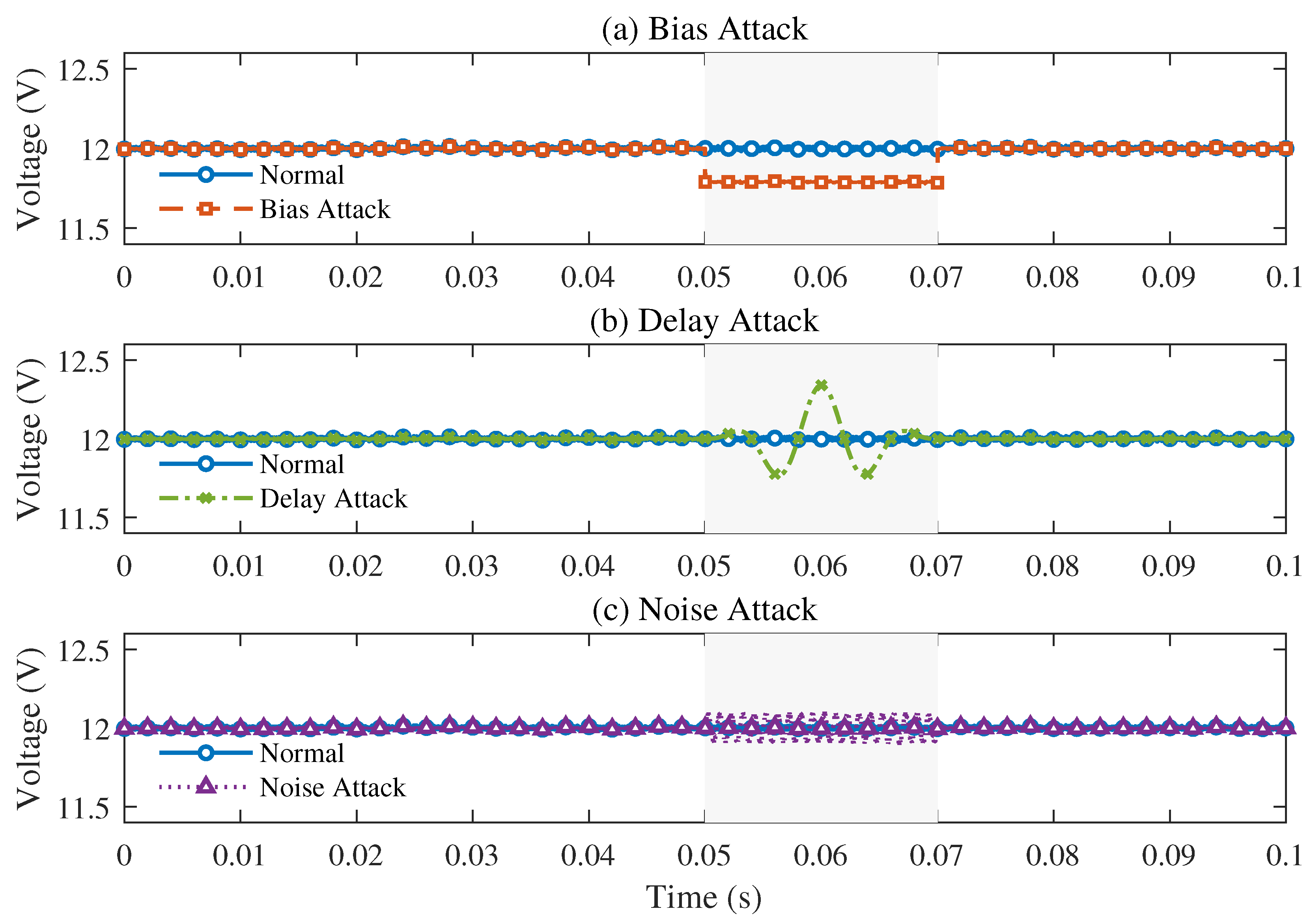
We evaluate three sensor-side attacks on the output voltage sensing path: (i) DC bias, (ii) fixed-sample delay via a ring buffer, and (iii) narrowband sinusoidal injection (1 kHz). Unless otherwise noted, the sampling period is Δ t = 10 µs and the attack window is 50–70 ms. Implementations are summarized in Algorithms 1–3 [28,29,30].
Algorithm 1 Bias attack (voltage only, physically consistent)
  1:
Inputs:
  2:
    v true [ 0 : T 1 ]                    ▹ true output voltage
  3:
    α fb           ▹ feedback divider ratio (e.g., 12 3.3  V α fb 0.275 )
  4:
    δ cmd     ▹ commanded bias magnitude (e.g., + 0.4  V at the injection origin)
  5:
    site { post _ divider , pre _ divider , digital }
  6:
    ( n on , n off )             ▹ attack window in samples (e.g., 50–70 ms)
  7:
Define the effective gain to the feedback node:
g site = 1 , post_divider α fb , pre_divider γ dig , digital (calibrated path gain)
  8:
δ eff g site δ cmd                        ▹ offset at v f b
  9:
Δ v meas δ eff / α fb            ▹ equivalent offset on the V out channel
10:
for n = 0 to T 1 do
11:
    if  n on n n off  then
12:
         v atk [ n ] v true [ n ] + Δ v meas
13:
    else
14:
         v atk [ n ] v true [ n ]
15:
    end if
16:
end for
17:
Output: v atk [ 0 : T 1 ]
Algorithm 2 Delay attack (ring buffer at sampling period Δ t )
1:
Input: raw sequence s orig [ 0 : T 1 ] , sampling period Δ t , desired delay τ d
2:
N max { 1 , round ( τ d / Δ t ) }               ▹ delay length in samples
3:
Init: B [ 0 : N 1 ] s orig [ 0 ]                     ▹ startup fill
4:
for n = 0 to T 1 do
5:
     s del [ n ] B [ n mod N ]                  ▹ read delayed sample
6:
     B [ n mod N ] s orig [ n ]                 ▹ write current sample
7:
end for
8:
Output: s del [ 0 : T 1 ]                    ▹ pure delay N Δ t
Algorithm 3 Noise attack (narrowband sinusoidal injection)
1:
Parameters: Δ t = 10 μ s, T samples, f atk = 1  kHz, V pp = 0.5  V
2:
A atk V pp / 2
3:
for n = 0 to T 1 do
4:
     n atk [ n ] A atk sin 2 π f atk n Δ t
5:
     s noisy [ n ] s orig [ n ] + n atk [ n ]
6:
end for
7:
Output: s noisy [ 0 : T 1 ]

2.2.1. Bias Attack Modeling

A DC bias is injected on the voltage-sensing channel with scaling determined by the feedback divider and the injection site.
Note. With integral action (no saturation), the steady-state output shift follows Δ V out δ eff / α fb ; a positive bias at v f b causes the controller to perceive a higher voltage, reducing the duty and lowering V out .

2.2.2. Delay Attack Modeling

A fixed sensor path delay is realized by inserting a ring buffer operating at the sampling period.
Note. The effective pure delay is τ d N Δ t . In experiments, we used f s = 1 / Δ t = 100  kHz and N = 102 ( τ d 1.02  ms).

2.2.3. Noise Injection Attack Modeling

Periodic interference is emulated by superimposing a narrowband sinusoid on the sensed voltage (or current).

2.2.4. Rationale for Attack Parameter Choices

Narrowband jamming at 1 kHz. (i) The tone lies inside the voltage loop bandwidth and well below the inference Nyquist (10 kHz/2), producing a measurable closed-loop response without aliasing; (ii) at f inf = 10  kHz with L = 30 (3.0 ms window), 1 kHz provides ≈3 cycles per decision window, stabilizing the score; (iii) it is spectrally far from switching harmonics at k f sw (100 kHz, k 1 ), so its effect appears in time-domain ripple V r , p p and regulation rather than the IRR defined around k f sw bands.
Fixed delay τ 1.02  ms. Implemented by a ring buffer of length N = 102 at f s = 100  kHz, this value purposefully erodes the phase margin to reveal the low-frequency modulation (∼120–130 Hz) predicted by ϕ delay ( f ) = 360 f τ and corroborated in the hardware, while remaining safe for the rig.
Bias magnitude. The commanded offset was chosen so that the effective feedback-node bias yields a steady-state output shift Δ V o u t δ eff / α fb 0.21  V at 12 V (about 1.75 % ), i.e., near but within the ± 2 % regulation limit, exercising the detector without violating the safety box.
Attack window (50–70 ms) and amplitude. A 20 ms window covers ∼20 cycles at 1 kHz and allows a consistent latency estimate under the N = 3 rule; amplitudes are set so that the closed-loop V r , p p and DC regulation remain within the limits in the no CI actuation hardware runs.
Figure 1 summarizes the pathway from physical sensor manipulation to the internal control response.

2.2.5. Real-World Scenarios (EV/PV/ESS)

We consider field-plausible disturbances that affect the same safety box metrics ( V r , p p , IRR, ±2% regulation) and the detector’s score: (i) supply-side ripple/jamming on V i n (hundreds of Hz–few kHz; within loop bandwidth), (ii) sensor bias/drift at the divider or ADC path, (iii) a fixed sensor path delay from buffering/firmware (sub-ms–few ms), (iv) narrowband EMI on sense lines (e.g., ∼1 kHz). All cases are evaluated with the same decision rule ( τ = μ + 3 σ , N = 3 ).
Real-world scenarios and their primary effects are summarized in Table 4.

2.3. Physics-Informed LSTM Model Structure

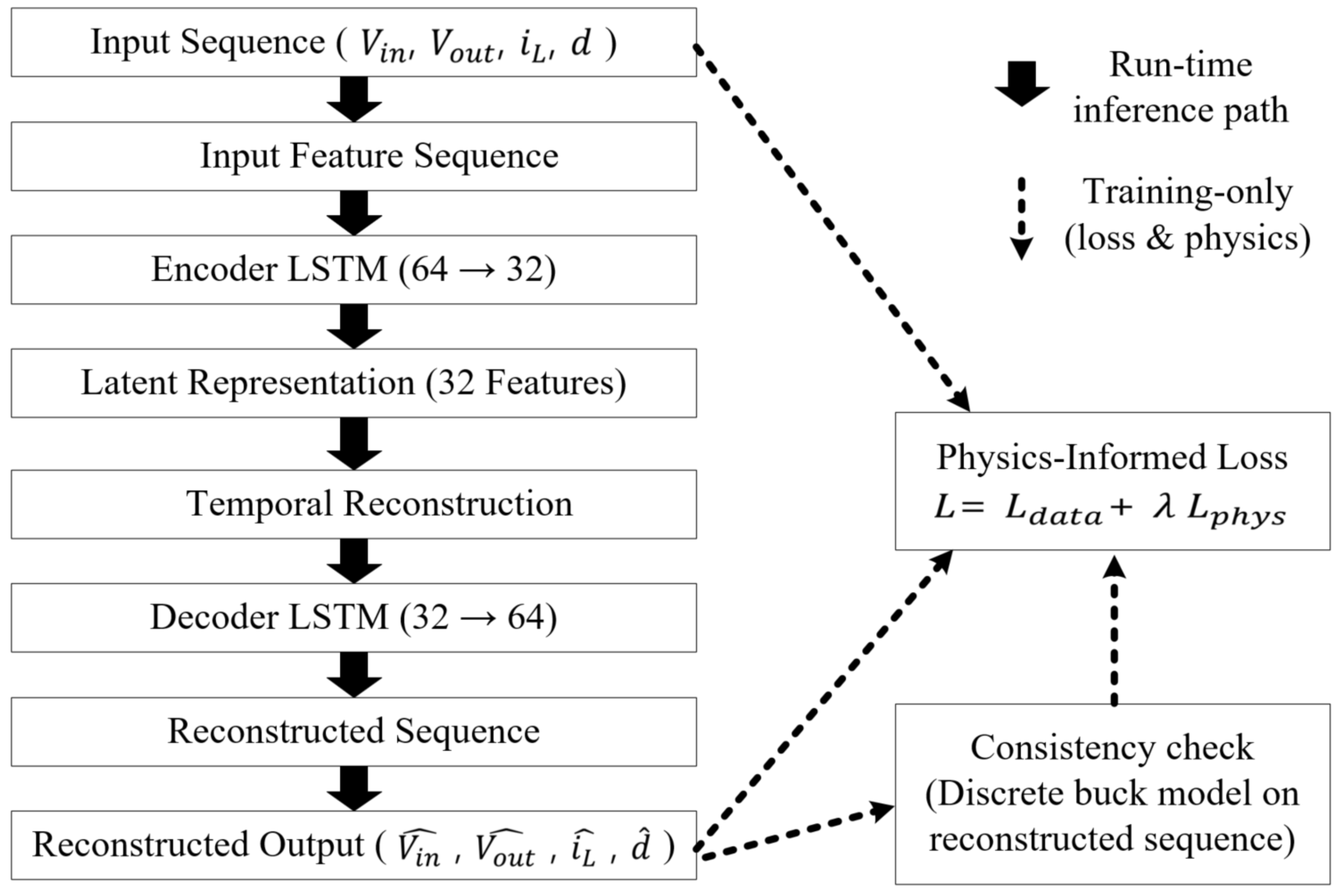
We adopt an LSTM autoencoder that embeds the buck converter physics as discrete-time residual constraints. The offline model uses an encoder (64→32) and a decoder (32→64) with input window length L = 30 samples. For real-time deployment, we use a distilled single-layer PI–LSTM ( n x = 4 , n h = 32 ) derived from the same objective [31,32,33].

2.3.1. Time-Base Convention (Simulation vs. Hardware)

The simulation uses the controller-rate stream with Δ t  = 10 µs ( f s = 100  kHz) and  L = 30 (window 0.30  ms). On hardware, the ADC runs at 100 kHz but inference uses decimation by M = 10 ( f inf = 10  kHz), so the same L = 30 spans 3.0  ms. Decisions advance every 0.1  ms and adopt an N = 3 consecutive-samples rule (lower-bound add-on 0.2  ms).
Figure 2 shows the architecture of the proposed PI–LSTM autoencoder.
The training hardware, dataset size, optimization settings, wall clock time, and memory footprint are summarized in Table 5.

2.3.2. Hyperparameter Selection and Validation Protocol

Invariants. The decision rule (threshold τ = μ + 3 σ from benign data; N = 3 consecutive samples) and the input window L = 30 were fixed to preserve real-time latency and ensure fair comparison across methods.
Search space. We considered hidden size n h { 16 , 32 , 64 } , physics weight λ phys { 0 , 0.05 , 0.10 , 0.20 } , batch size { 64 , 128 } , initial learning rate { 10 3 , 5 × 10 4 } with either cosine decay to 10 4 or a 0.1 step at 75% of the max epochs, dropout { 0 , 0.1 } (on the LSTM output), weight decay { 0 , 10 5 } , and optimizer { Adam ( β 1 = 0.9 , β 2 = 0.999 ) , SGD ( mom . = 0.9 ) } .
Protocol. Data were split 80/10/10 (train/val/test). For each candidate, we trained up to 80 epochs with early stopping (patience 10). Model selection used the validation macro-F1 (averaged over the three attacks) under the constraint “alarm-wise FPR 2 % ”; latency served as a tiebreaker. Each configuration was repeated with three random seeds; we chose the median performer.
Chosen configuration. Adam with cosine decay (initial 10 3 10 4 ), batch 128, n h = 32 , λ phys = 0.10 , dropout 0, weight decay 10 5 . This offline model is then distilled to the runtime single-layer PI–LSTM ( n x = 4 , n h = 32 ) used on the DSP (Section 4.2).

2.3.3. Cross-Validation and Leakage Control

Fold construction. We use grouped, stratified 5-fold cross-validation on the simulation corpus. Folds are created at the run/trajectory level (not per window) to prevent temporal leakage; class balance (benign vs. each attack) and operating point diversity are preserved across folds.
Per-fold protocol. For each fold, models are trained on 4 folds with early stopping (patience 10). The decision rule is identical to deployment: threshold τ = μ + 3 σ computed from benign data of the training side only and an N = 3 consecutive-samples policy. Hyperparameters follow the selected configuration (Adam with cosine decay, n h = 32 , λ phys = 0.10 , batch 128), i.e., we assess the generalization of the chosen setting rather than retuning in each fold.
Reporting. We aggregate per-fold metrics as mean ±95% confidence intervals: macro-F1 (averaged over bias/delay/noise), alarm-wise FPR, and detection latency (median [IQR]). A 5-fold outcome is macro-F1 94.9 ± 0.6 % , FPR 1.0 ± 0.3 % , and latency 3.2  ms [2.8–3.9] under the fixed rule. Hardware results remain reported separately and unchanged.
Inputs/outputs. Inputs are [ V in , V out , i L , d ] ; the decoder reconstructs [ V in ^ , V out ^ , i L ^ , d ^ ] . The anomaly score is the reconstruction error; the decision rule is fixed ( τ = μ + 3 σ , N = 3 ).
Discrete-time physical constraints (no label leakage). Let N b denote the number of time steps summed over a batch. The total loss is the weighted sum of data loss and physics residual loss; residuals are evaluated on decoder outputs at k and k + 1 :
L total = L data + λ phys L phys , L phys = 1 N b k = 0 N b 2 V out ^ [ k + 1 ] V out ^ [ k ] Δ t C i L ^ [ k ] V out ^ [ k ] R 2
+ i L ^ [ k + 1 ] i L ^ [ k ] Δ t L V in ^ [ k ] d ^ [ k ] V out ^ [ k ] 2 .
We use λ phys = 0.1 . (Optionally, midpoint collocation between k and k + 1 can be added to reduce discretization errors).

2.4. Physics-Informed Learning Framework

The PI–LSTM enforces the discrete-time converter dynamics during training, which (i) improves generalization beyond the training distribution, (ii) reduces noise sensitivity, and (iii) enhances interpretability by checking the physical consistency of reconstructions. The discrete-time formulation aligns with fixed-step Simulink solvers and is compatible with real-time deployment [34,35,36].

Context in the Broader PINN Literature

Physics-informed learning has been widely adopted beyond power electronics, e.g., forward/inverse PDEs in fluids and solids [15,16,17,18], with landmark demonstrations such as hidden fluid mechanics [19]. More broadly, theory-guided data science argues for embedding domain constraints directly into learning objectives [20]. Our PI–LSTM follows the same principle by enforcing discrete-time circuit residuals (rather than continuous PDEs), aligning with fixed-step control implementations.

2.5. CI-Guided Intentional Performance Degradation (Unified with DC Rail Ripple Metrics)

When the anomaly score s k exceeds the threshold τ for N consecutive samples, we enable a safety-bounded performance adjustment. The confusion index (CI) aggregates efficiency deviation and DC rail ripple metrics (time-domain V r , pp and frequency-domain IRR ) using normalizers identical to the safety box limits [37,38]:
z = [ η , V r , pp , IRR ] , η = nominal efficiency , p η = clip η η η , 0 , 1 , p r , time = clip V r , pp 240 mV , 0 , 1 , p r , freq = clip IRR 2 % , 0 , 1 , CI = w η p η + w r , time p r , time + w r , freq p r , freq , w η + w r , time + w r , freq = 1 .
Safety box (also used as CI normalizer).
| V out V | ± 2 % , V r , pp 240 mV , IRR 2 % , I L rms I max , T j T j , max .
IRR convention. Unless otherwise noted, the IRR is computed via the Welch PSD (Hann, 50% overlap) integrating ± Δ f = 0.5  kHz around the first K = 5 switching harmonics; the same ( Δ f , K ) and limit 2 % are used in both the safety box and CI.
Actuation law (bounded by safety margins).
α = sat ( CI ) , α [ 0 , α max ] , V ref V ref ( 1 k v α ) , d d ( 1 k d α ) , f s w f 0 ( 1 ± k f α ) ,
with immediate backoff when any constraint in Equation (6) approaches violation.
The CI-guided deception routine under the unified safety box is summarized in Algorithm 4.
Algorithm 4 CI-guided deception under a unified safety box
Require: 
score s k , threshold τ , persistence N, hysteresis T hys
  1:
if s k N + 1 , , s k > τ then
  2:
     p η clip ( ( η η ) / η , 0 , 1 )
  3:
     p r , time clip ( V r , pp / 240 mV , 0 , 1 )
  4:
     p r , freq clip ( IRR / 2 % , 0 , 1 )
  5:
     CI w η p η + w r , time p r , time + w r , freq p r , freq
  6:
     α sat ( CI )                           ▹ α [ 0 , α max ]
  7:
     V ref V ref ( 1 k v α ) ;    d d ( 1 k d α ) ;    f s w f 0 ( 1 ± k f α )
  8:
    if any limit in Equation (6) is near violation then  α β α end if   ▹ 0 < β < 1
  9:
else
10:
    if  s k < τ for T hys then ramp α 0 and restore nominal settings end if
11:
end if
The unified CI weights, ripple limits, and actuation gains are listed in Table 6.

3. Simulation Results and Analysis

3.1. Simulation Environment Setup

Simulations were conducted in MATLAB R2024a. Key settings are summarized in Table 7.

Classical Baselines (EKF Residual and Shewhart)

EKF residual. Using the averaged buck model, the innovation r k = y k C x ^ k | k 1 with covariance S k = C P k | k 1 C + R yields the normalized statistic z k = r k S k 1 r k . A binary alarm is raised when z k exceeds a fixed threshold τ = μ + 3 σ estimated from benign data, with an N = 3 consecutive-samples rule (identical to PI–LSTM).
Shewhart detector. As a lightweight classical baseline, we apply a Shewhart test on the scalarized residual norm r k 2 (or an equivalent sample-wise statistic) using the same decision policy (see Section 4.3 for the fixed decision rule). Both baselines use exactly the same signal windows, normalization, and evaluation metrics as for PI–LSTM (F1, alarm-wise FPR, latency), ensuring a fair comparison.
Figure 3 shows deviations from the nominal trajectory for the three sensor-side attacks. The mean detection latencies reported later in Table 8 (2.88 ms, 3.95 ms, 2.59 ms for bias, delay, noise) are computed as the arithmetic mean over n = 1000 runs; the corresponding standard deviations ( ± 0.15 0.22 ms) confirm statistical consistency under the fixed decision rule above.

3.2. Benchmark Dataset Domain Alignment (Auxiliary Evaluation)

We primarily evaluate in-domain (DC–DC buck converters) data from simulations and our DSP-based prototype. To probe cross-domain generalization on public data, we additionally use an inverter-driven PMSM dataset (Zenodo) [39]. Because the PMSM domain differs from a DC–DC buck, we treat it strictly as an auxiliary benchmark and apply the following protocol before training/evaluation.
1.
Signal mapping. Select PMSM signals that are physically analogous to our inputs [ v in , v out , i L , d ] (e.g., DC bus voltage/current and duty or normalized gate command). Exclude non-analogous mechanical variables from the core feature set.
2.
Sampling (no upsampling). Use all PMSM signals at their native 10 Hz sampling rate (no upsampling or resampling). Apply per-window mean removal (AC coupling) and z-score normalization computed on benign segments. The decision rule is identical to the buck study: threshold τ = μ + 3 σ and an N = 3 consecutive-samples policy.
3.
Attack semantics. When labels exist (bias/delay/noise), retain them. Otherwise, inject attacks consistent with our threat model (bias at the sensor tap; fixed-sample delay; a narrowband sinusoid at a frequency resolvable under 10 Hz Nyquist) to preserve semantic alignment.
4.
Metrics separation. DC rail power quality metrics ( V r , pp , IRR) are not computed for PMSM. We report only detection metrics (accuracy, F1, AUC, alarm-wise FPR) for PMSM, and we do not compare the absolute latencies between the PMSM and buck domains.
We emphasize that all principal claims (e.g., safety box compliance and CI analysis) are supported by the buck domain. The PMSM results serve only as an auxiliary generalization check under a standardized preprocessing pipeline.

3.2.1. Auxiliary PMSM Dataset: Sampling Rate Disclosure and Verification

To avoid ambiguity about the public PMSM drive dataset used in the auxiliary evaluation, we explicitly consume it at its native time base. We verified from the provided time stamps that the inter-sample interval was effectively constant at Δ t = 0.10 s (10 Hz) up to file-level rounding tolerance. Accordingly, we perform no upsampling/resampling; all preprocessing (per-window mean removal; z-score normalization on benign segments) operates on the 10 Hz stream. When labels are absent and synthetic perturbations are injected to align with our threat model, their frequencies are chosen to be resolvable under the 5 Hz Nyquist limit (i.e., f atk < 5 Hz) with durations exceeding three periods. As emphasized in the main text, DC rail quality metrics ( V r , p p , IRR) and millisecond-scale latency are not computed for this dataset; only detection metrics are reported.

3.2.2. Detector Configuration at Low Rate

For PMSM, the detector window is L = 30 samples at 10 Hz (3.0 s). With the same N = 3 rule, the alarm persistence is approximately 0.3 s.

3.3. Attack Detection Performance Analysis

We evaluate the detection performance for each attack via Monte Carlo simulation with n = 1000 runs per attack type [40,41]. Table 8 reports aggregate metrics.
Classical detectors under the identical decision protocol are summarized in Table 9.

Additional Baselines: SVM and Random Forest

Featurization and fairness. For classical classifiers, each window ( L = 30 ) is vectorized by stacking the [ V in , V out , i L , d ] samples (z-scored per channel), yielding a 4 × 30 vector. SVM (linear) and random forest (200 trees, depth 8 ) are trained in a supervised manner on benign/attack labels; decisions follow the same alarm policy (see Section 4.3 for the fixed decision rule); the class score threshold is 0.5. Windows, normalization, and metrics match those for PI–LSTM.
Windowed classifiers (SVM, RF) under the identical decision protocol are summarized in Table 10.
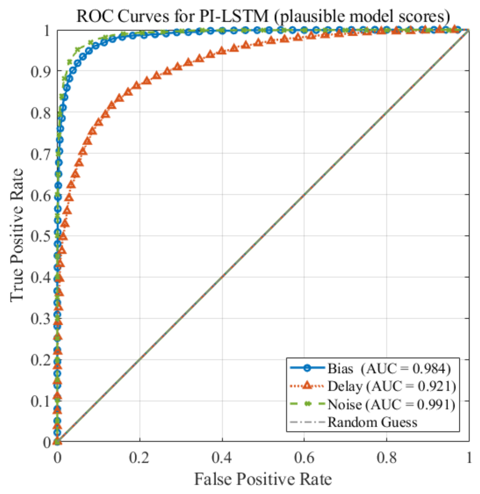
ROC summary. AUCs are 0.984 (bias), 0.921 (delay), and 0.991 (noise); delay is comparatively harder to detect. Under the same decision rule, the alarm-wise false-positive rates in the simulation are 0.8% (bias), 1.2% (delay), and 0.6% (noise); hardware measurements are ≤1.2% (see Section 4.3).
Figure 4 shows the ROC curves of the PI–LSTM for the three attacks; the AUCs are 0.984 (bias), 0.921 (delay), and 0.991 (noise), indicating that the delay is comparatively harder to determine. The diagonal line marks random guessing; curves closer to the upper-left corner indicate better detection.
Figure 5 shows clear benign/attack separation relative to the benign-only threshold ( τ = μ + 3 σ ; Section 4.3); the delay exhibits the largest overlap, consistent with the lower AUC. In Figure 6, latencies are ordered as noise < bias < delay with tight IQRs over n = 1000 runs, aligning with Table 8.

3.4. Public Benchmark Comparison

For auxiliary validation, we use the Comprehensive Dataset for Fault Detection and Diagnosis in Inverter-Driven PMSM Systems (Zenodo) [39]. This PMSM drive dataset provides multi-sensor measurements at a native 10 Hz sampling rate across multiple operating conditions and fault modes. We treat it strictly as a cross-domain benchmark: signals are used at their native rate (no upsampling), channels are standardized (z-score on benign segments) with per-window mean removal, and we report detection metrics only (accuracy, F1, AUC, alarm-wise FPR). No V r , pp , IRR, or millisecond latency comparisons are computed for this dataset [42,43].
We compare four methods:
  • ARIMA (residual μ + 3 σ threshold);
  • Isolation Forest (100 trees, 4 features);
  • CNN–LSTM Autoencoder (1D-CNN→LSTM; reimplementation of [44]);
  • Proposed PI–LSTM ( λ physics = 0.1 ).
Hyperparameters (batch size {64, 128}, learning rate { 10 3 , 10 4 }) are selected by grid search. Each method is evaluated over five independent training trials; we report the mean and 95% confidence intervals (AUC CIs via bootstrap, B = 1000 ).
The auxiliary PMSM benchmark with classical baselines (native 10 Hz, no upsampling) is summarized in Table 11.
The auxiliary PMSM benchmark (native 10 Hz, no upsampling) is summarized in Table 12.
The proposed PI–LSTM improves the F1 by 4.0–12.2 percentage points and the AUC by 0.026–0.075 versus the baselines, while more than halving the alarm-wise FPR relative to ARIMA/isolation forest, indicating robust cross-domain generalization under a consistent decision rule [45,46].

3.5. CI-Guided Deception Under a Unified Safety Box (Simulation Only)

Normalization and limits follow the unified safety box and CI definitions. See Section 2.5, Equations (5) and (6). The decision rule matches detection (threshold τ = μ + 3 σ , N = 3 , refractory T hys = 10 ms).
Canonical reference. All mentions of the “safety box”, its limits/normalizers, and CI normalization elsewhere in the paper refer to Equations (5) and (6) in this subsection.
CI weighting: rationale and sensitivity. Weights ( w η , w r , time , w r , freq ) prioritize safety box margins while penalizing efficiency loss; the baseline ( 0.5 , 0.3 , 0.2 ) in Table 6 reflects (i) user-visible ripple ( V r , pp ), (ii) spectral in-band content (IRR), and (iii) energy overhead via p η . We ablate alternative weightings at the operating point used in Table 13.
CI sensitivity to weight choices at the representative point is summarized in Table 14.
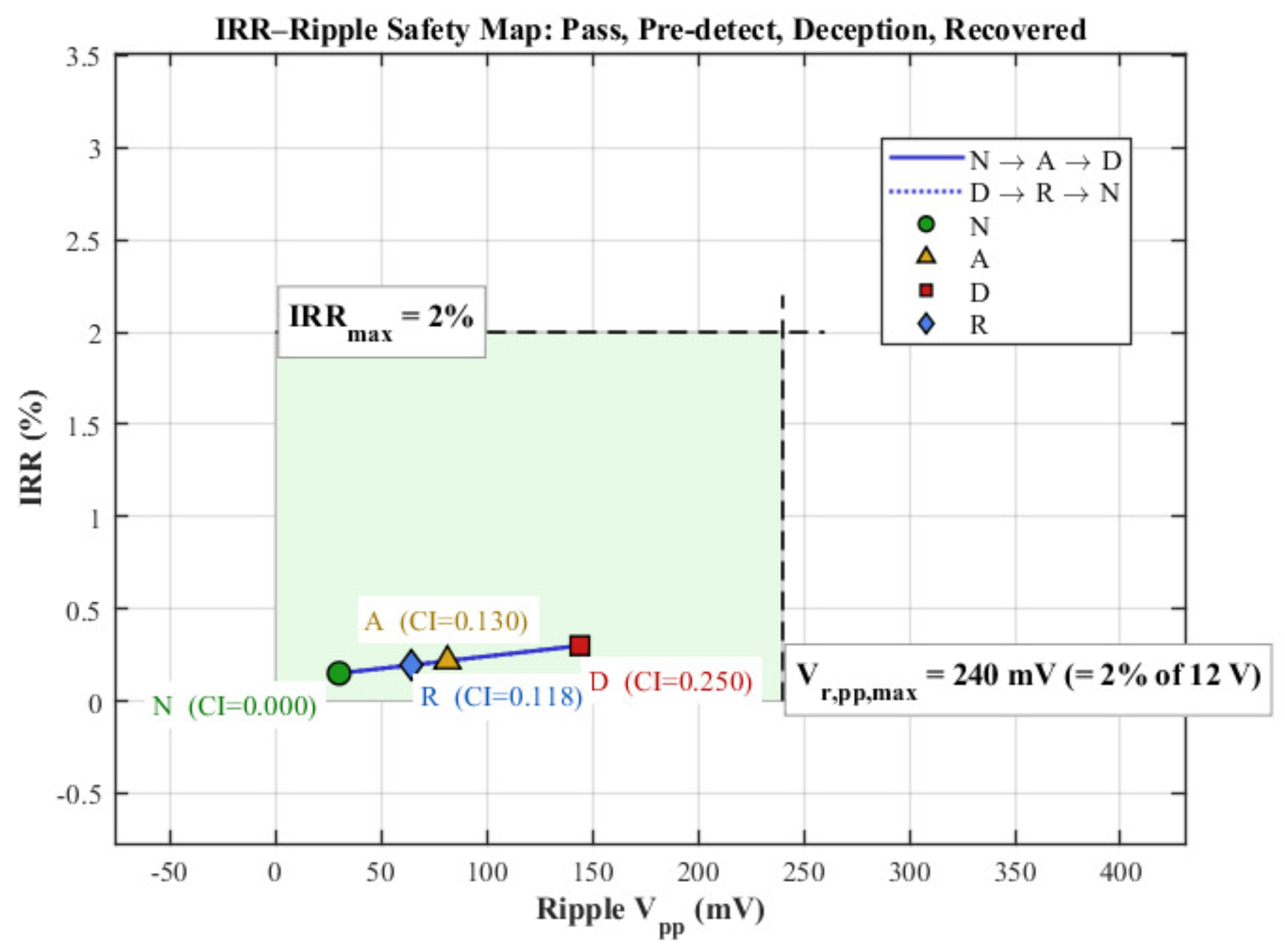
Figure 7 shows that, under CI-guided actuation, the trajectory remains within the unified safety box and returns to the nominal region after the attack. See Section 2.5, Equations (5) and (6). Letter markers denote phases (N: nominal; A: under attack; D: actuation engaged; R: recovery). Actuation is triggered when CI > τ for N = 3 consecutive samples and then drives the operating point toward lower V r , pp and lower IRR until re-entry; after release with hysteresis, the point returns to N. Short segments near A and R may visually overlap due to the sampling step; the letter markers disambiguate the phase transitions even when path segments appear superimposed.

Scope and Hardware Linkage

The hardware experiments in this paper validate the detection path only (latency/FPR). Without CI actuation on hardware, the V r , pp and IRR stayed within the limits, while the ± 2 % regulation window was occasionally exceeded under delay (peak 2.8 % ; see Section 4.3). Demonstrating CI-guided actuation under the full safety box on hardware is left to future work.

3.6. Effect of Physical Constraints

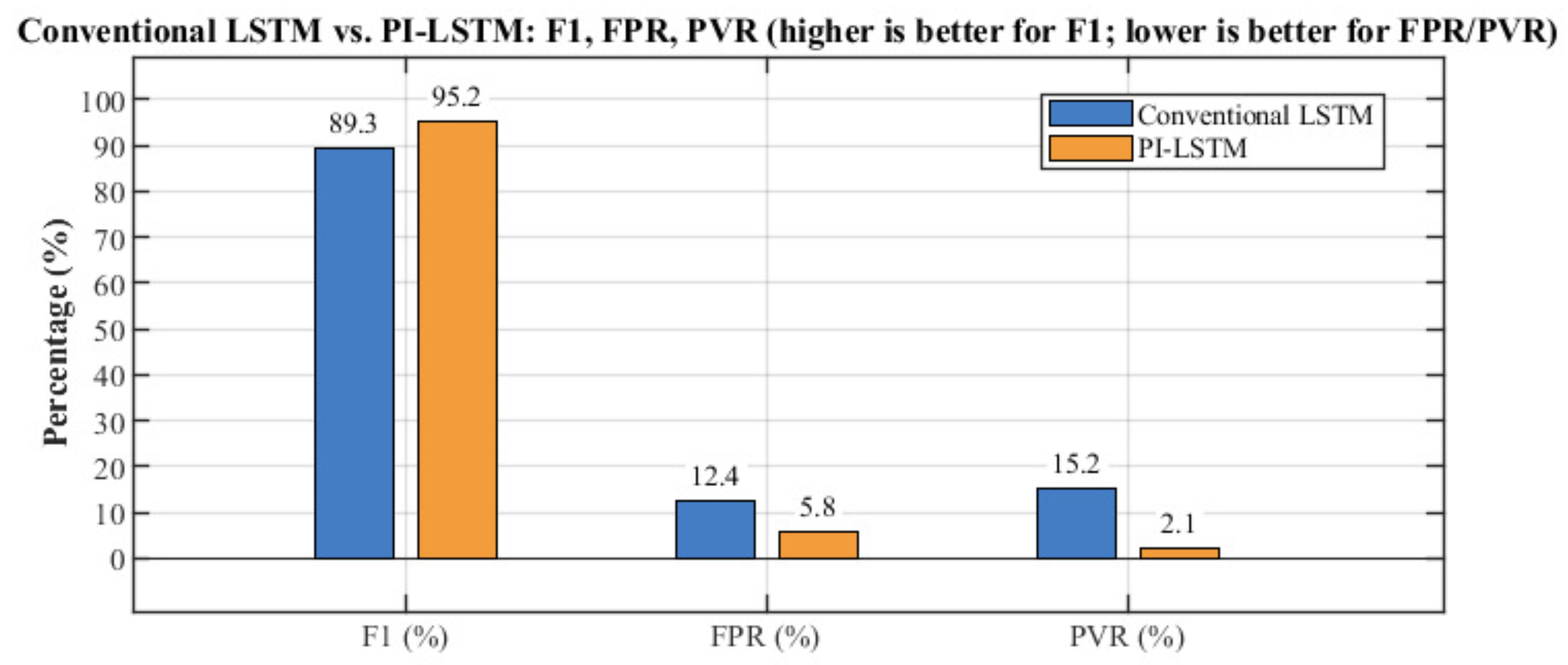
We compare a conventional data-driven LSTM with the proposed physics-informed LSTM (PI–LSTM) to quantify the benefit of enforcing discrete-time converter dyna- mics [47,48]. Table 15 reports average test metrics; “FPR” is the alarm-wise false-positive rate with the N = 3 consecutive-samples rule, and “PVR” (physical violation rate) is the fraction of time steps whose reconstructions violate the discrete-time residual constraints beyond a fixed tolerance.
Figure 8 summarizes the aggregate test metrics for the two models. Consistent with Table 15, the PI–LSTM attains a higher F1 score (95.2 vs. 89.3) and substantially lower false-positive rate (5.8% vs. 12.4%) and physical violation rate (2.1% vs. 15.2%). Interpreting the axes, higher is better for the F1, whereas lower is better for the FPR and PVR. The relative changes shown in Equations (8)–(10) quantify these gains.
Relative changes are as follows:
F 1 improvement = 95.2 89.3 89.3 × 100 % 6.61 % ,
FPR reduction = 12.4 5.8 12.4 × 100 % 53.23 % ,
PVR reduction = 15.2 2.1 15.2 × 100 % 86.18 % .
These results indicate that the PI–LSTM improves the anomaly detection accuracy while substantially lowering false alarms and physics law violations, supporting deployability on real hardware [49,50].
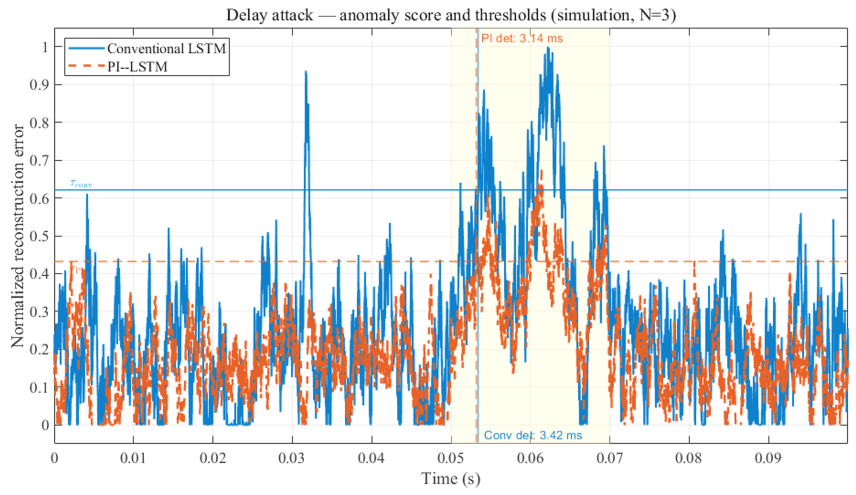
Figure 9 contrasts the normalized reconstruction error trajectories of a conventional LSTM and the proposed PI–LSTM under a delay attack at f s = 100 kHz with window L = 30 ( N = 3 rule). The PI–LSTM exhibits fewer spurious excursions above its threshold, consistent with the lower FPR in Table 15.

4. Experimental Setup and Results

4.1. Experimental Setup

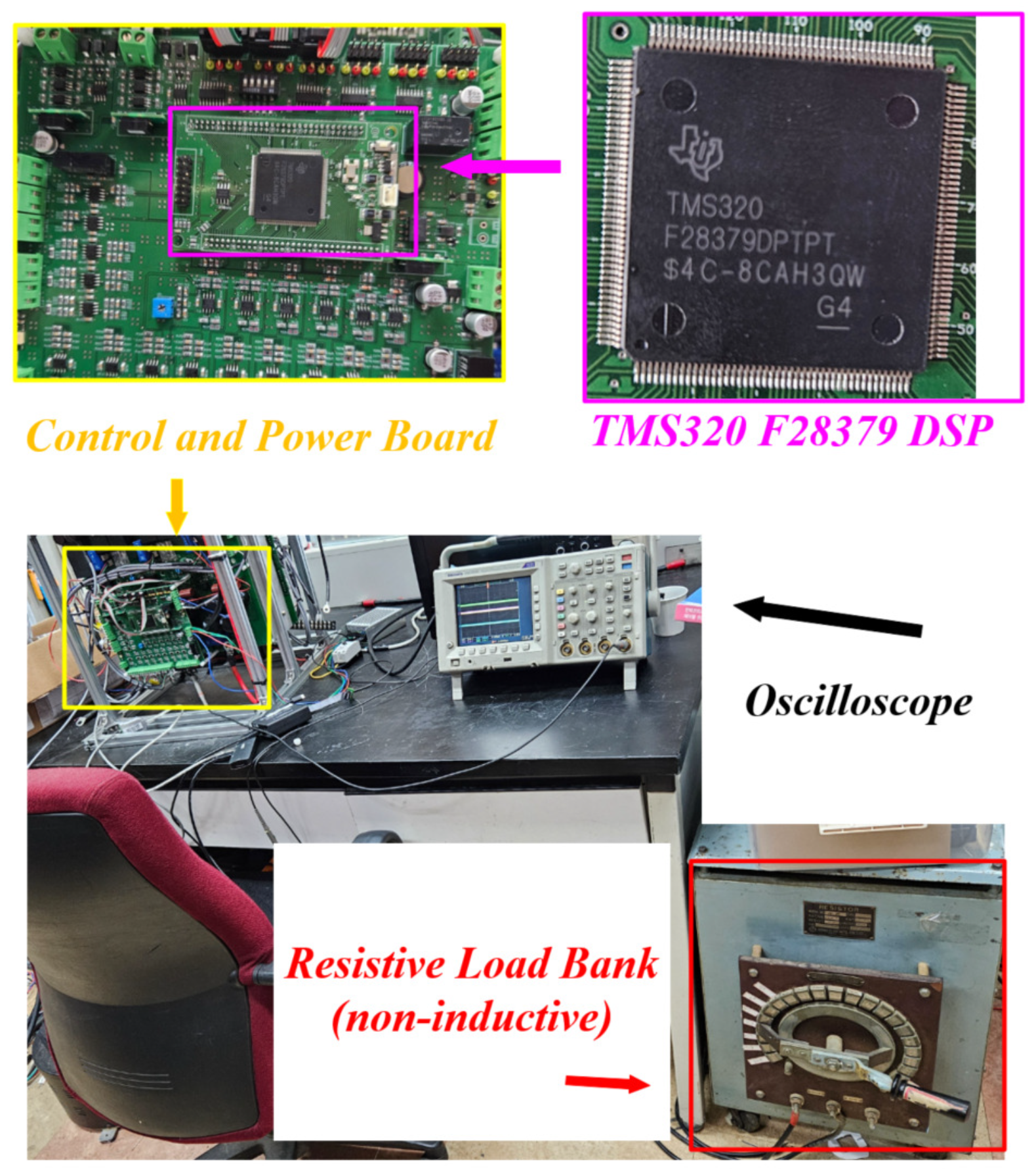
A 24 V→12 V buck converter prototype was built to validate the simulation findings. Hardware parameters matched the simulation: V i n = 24 V, V o u t = 12 V, R load 10 Ω , f s w = 100 kHz (CCM), L = 100 µH, and C = 470 µF. Figure 10 shows the experimental setup used for hardware evaluation.
Real-time inference ran on a TMS320F28379 DSP. We deployed a distilled single-layer PI–LSTM ( n x = 4 , n h = 32 ) on a decimated stream ( M = 10 , f inf = 10 kHz). The anomaly score is the reconstruction error. We use the same decision rule as in the simulation ( τ = μ + 3 σ , N = 3 ), with hysteresis T hys = 10 ms. Sensing used isolated differential amplifiers for v o u t and a Hall effect sensor for i L . Signals were sampled at f s = 100 kHz and processed in FP32. Matrix multiplications used DSPLib; activations used branch-free piecewise-linear approximations. The DSP TMU was not used for neural activations [51,52].
We injected three sensor path attacks with an auxiliary module placed between the sensors and the ADC:
1.
DC bias with calibrated mapping to the feedback path;
2.
Fixed sample delay τ 1.02 ms (FIFO at f s = 100 kHz);
3.
Narrowband sinusoidal injection at 1 kHz ( 0.5 V pp ).

4.1.1. Measurement Protocol and Definitions

A DSO with a 20 MHz bandwidth limit was used under AC coupling for switching ripple ( V r , p p ), whereas DC coupling was used for DC regulation and for step/bias/delay tests. For frequency-domain assessment, the in-band ripple ratio (IRR) was computed from a Welch PSD (Hann, 50% overlap). Unless otherwise noted, we used Δ f = 0.5 kHz and K = 5 , a scope sampling rate ≥10 MS/s, and records ≥1 Mpts; the same ( Δ f , K ) are used in the confusion index (CI) calculation.
v ˜ o ( t ) = v o ( t ) ( a t + b ) , (local linear detrend on an AC-coupled gate)
V r , p p = max W v ˜ o min W v ˜ o , W : N sw = 5 10 periods
V inband , rms 2 = k = 1 K k f sw Δ f k f sw + Δ f S v v ( f ) d f ,
IRR = V inband , rms V out , DC .
Standard alignment for DC voltage quality and ripple. Our DC rail measurements follow widely used guidance: automotive DC voltage quality and superimposed ripple per ISO 16750-2 (electrical loads, including superimposed AC) [53] and ISO 21780 (48 V supply ranges and slow transients) [54]; product/EMC requirements for switch-mode PSUs per IEC 61204-3 [55]; and ripple/noise measurement practice using a 20 MHz oscilloscope bandwidth limit with local bypass at the connector, as in the Intel ATX12V design guide and oscilloscope vendor application notes. Accordingly, V r , pp is taken on an AC-coupled trace with a 20 MHz limit and a short ground spring, and the IRR is reported as a frequency-domain complement with explicit settings in Table 16. (To our knowledge, no formal standard defines IRR ; we therefore state its definition and parameters explicitly [56,57]).

4.1.2. Compliance and Interpretation

DC regulation uses the DC-coupled record: V out , DC is the mean of v o over an observation window (typically T reg 10 ms); a violation occurs if | V out , DC V | / V > 2 % . The ripple metrics V r , p p (Equation (12)) and IRR (Equation (14)) are evaluated on AC-coupled data as defined above with limits per the safety box. (See Section 2.5, Equations (5) and (6)). By construction, the IRR excludes low-frequency components (e.g., the 120–130 Hz component observed under the delay attack), which instead contribute to the DC regulation error.

4.2. Real-Time Inference Budget on TMS320F28379

This deployment is an architecture-reduced variant of the offline autoencoder in Section 2.3, keeping the same score definition and decision rule ( τ = μ + 3 σ , N = 3 ). Signals are sampled at f s = 100 kHz ( Δ t = 10 μ s); the streaming detector runs on a decimated stream with factor M = 10 ( f inf = 10 kHz) using a fixed window L = 30 (3.0 ms).

4.2.1. Analytic Complexity (per LSTM Layer)

For input size n x and hidden size n h ,
MAC / step = 4 n h ( n x + n h ) , # θ LSTM = 4 n h n x + n h 2 + n h ,
and ≈5 n h activation calls (four gates plus tanh ( c t ) ) per time step. Parameter memory is b · # θ with b = 4 B for FP32 (or 2 B for Q15).

4.2.2. Cycle Model

Let c mac be cycles per MAC for GEMM and c act be cycles per activation. The per-step cost is
C step c mac · MAC / step + c act · ( 5 n h ) .
For N L layers over a window of length L, C inf = 1 N L L C step ( ) [58].

4.2.3. Deployment Configuration (Example)

On a TMS320F28379 (200 MHz), we deploy a single-layer PI–LSTM with ( n x , n h ) = ( 4 , 32 ) in FP32, GEMM via DSPLib, and branch-free PWL activations. Using c mac 2.0 cycles/MAC and c act 10 cycles,
MAC / step = 4 · 32 · ( 4 + 32 ) = 4608 , 5 n h = 160 ,
C step 2.0 × 4608 + 10 × 160 11 kcycles 55 µ s / step at 200 MHz ,
within the 0.1 ms tick budget at f inf = 10 kHz. Parameter memory is 18.5 kB (FP32). The DSP TMU is not used for neural activations [52,59,60].

4.2.4. On-Board Measurement Protocol

We toggle a GPIO around lstm_step() and record the median over 10 4 calls with compiler optimizations enabled. Latency is reported in absolute time from attack onset; the simulation uses f s = 100 kHz with L = 30 ( 0.30 ms window), and hardware uses f inf = 10 kHz with the same L = 30 ( 3.0 ms window).
The DSP configuration and analytic compute/memory budget are summarized in Table 17.
On-board DSP deployment performance (TMS320F28379, 200 MHz) is summarized in Table 18.

4.2.5. Bias Injection and Scaling

Let the feedback divider be V f b = α fb V o u t with α fb = R 2 R 1 + R 2 (e.g., 12 V 3.3 V gives α fb 0.275 ). A software bias command δ cmd maps to an effective offset at the feedback node V f b as
δ eff = β δ cmd , analog injection after / before the divider β κ dig k ADC δ cmd , digital path via ADC codes , scaling κ dig / k ADC
where β = 1 if injected at V f b (post-divider) and β = α fb if injected pre-divider. Under integral action without saturation, the steady-state output shift follows
Δ V o u t δ eff α fb .
Example. In our setup, a + 0.4 V command yielded δ eff 58 mV at V f b and Δ V o u t 0.21 V, consistent with Equation (20).

4.2.6. Delay Injection: Implementation and Validation

A fixed pure delay is introduced in the sensing pipeline (ADC→DMA→ISR→PI) via a ring buffer of length N at sampling frequency f s :
τ est = N f s .
With f s = 100 kHz and N = 102 , we obtain τ est = 1.02 ms (≈100 T s for T s = 10 µs). Oscilloscope step-to-actuation timing (trigger at the reference step, measure gate driver change) gave
τ meas = 1.02 ± 0.03 ms ( n = 10 ) .
The additional phase lag from a pure delay is
ϕ delay ( f ) = 2 π f τ [ rad ] = 360 f τ [ deg ] ,
which reduces the phase margin and can excite low-frequency oscillation when loop crossover shifts downward under delay stress.

4.2.7. Oscilloscope and Probing Settings

Unless otherwise noted, waveforms were acquired as follows.
  • v o u t : 10:1 passive probe with spring ground; bandwidth limit 20 MHz. AC coupling for ripple ( V r , p p ); DC coupling for step/bias/delay tests.
  • i L : 20 MHz current probe, deskewed to the v o u t probe using a common step.
  • Time windows: ripple at 5–10 switching periods (50–100 μ s); low-frequency oscillation at 50–100 ms.
  • Triggering: rising edge of the attack window marker or reference step; memory depth ≥1 Mpts; sample rate ≥10 MS/s (ripple captures often at 200 MS/s).

4.3. Detection Metrics: Latency and False Positives

Let s [ n ] denote the anomaly score sampled at Δ t = 1 / f s . A fixed threshold τ is set from benign validation data as τ = μ + 3 σ . Decisions use an N-consecutive rule with an optional refractory period T hys
alarm at n s [ n + i ] τ i = 0 , , N 1 ,
and, once an alarm is issued, further alarms are suppressed for T hys .

4.3.1. Detection Latency

Let t 0 be the known attack onset and t a the earliest time index that satisfies the N-consecutive rule. The detection latency is
t d = t a t 0 .

4.3.2. False Positive Rate (Alarm-Wise)

Over a collection of attack-free evaluation units U B (simulation runs of fixed length or non-overlapping benign windows),
FPR ( % ) = 1 | U B | u U B 1 n u : s [ n + i ] τ i = 0 , , N 1 × 100 .
This measures how often a false alarm occurs on benign data under the same decision rule.

4.3.3. Sample-Wise Exceedance (Secondary Descriptor)

For completeness, we also report the sample-wise positive fraction (SPF),
SPF ( % ) = 1 | B | n B 1 s [ n ] τ × 100 ,
where B is the set of benign samples. The SPF characterizes score distributions but is not used as the FPR in the main text.

4.3.4. Statistical Reporting Conventions

We report means with 95% confidence intervals and use Wilson intervals for proportions and bootstrapping for the AUC; full details are provided in Supplementary File S1.

4.3.5. System-Level Impact and Resilience Metrics

Beyond the F1 and alarm-wise FPR, we report system-level KPIs that reflect efficiency, stability margins, and long-term resilience under attacks and CI actuation, using the same measurement records as for V r , pp , IRR , and regulation.
Efficiency and energy overhead. Let η be the benign baseline and η the value under attack/CI; we track Δ η = η η and a normalized penalty p η = ( η η ) / η . Over a window T w , the energy overhead is E over = t t + T w P in ( 1 η ) d t t t + T w P in ( 1 η ) d t .
Stability proxies. We monitor a delay-sensitive low-frequency component induced by a fixed sensor path delay: the oscillation index OI 100 150 Hz is the RMS of the 100 150 Hz band of v out , normalized by V out , DC . As a surrogate lower bound on the phase margin, PM lb 180 360 f c τ est with loop bandwidth f c (from step/PRBS identification) and delay estimate τ est (from ring buffer or timing).
Resilience (fleet/O&M). We track the alarm density AD = N alarms / T obs on benign operation, the mean time between alarms MTBA = T obs / N alarms , the mean time to recovery MTTR (alarm onset → within-limit restoration), and the score drift index SDI = | μ s μ s , ref | / σ s , ref on verified benign segments (shadow mode), which guides periodic rethresholding.
System-level KPIs used in addition to detection metrics are summarized in Table 19.
These KPIs complement the F1/AUC/FPR by quantifying efficiency impacts, stability margin erosion, and operational resilience; they align with the safety box and CI normalization already used in this work.

4.4. Experimental Results

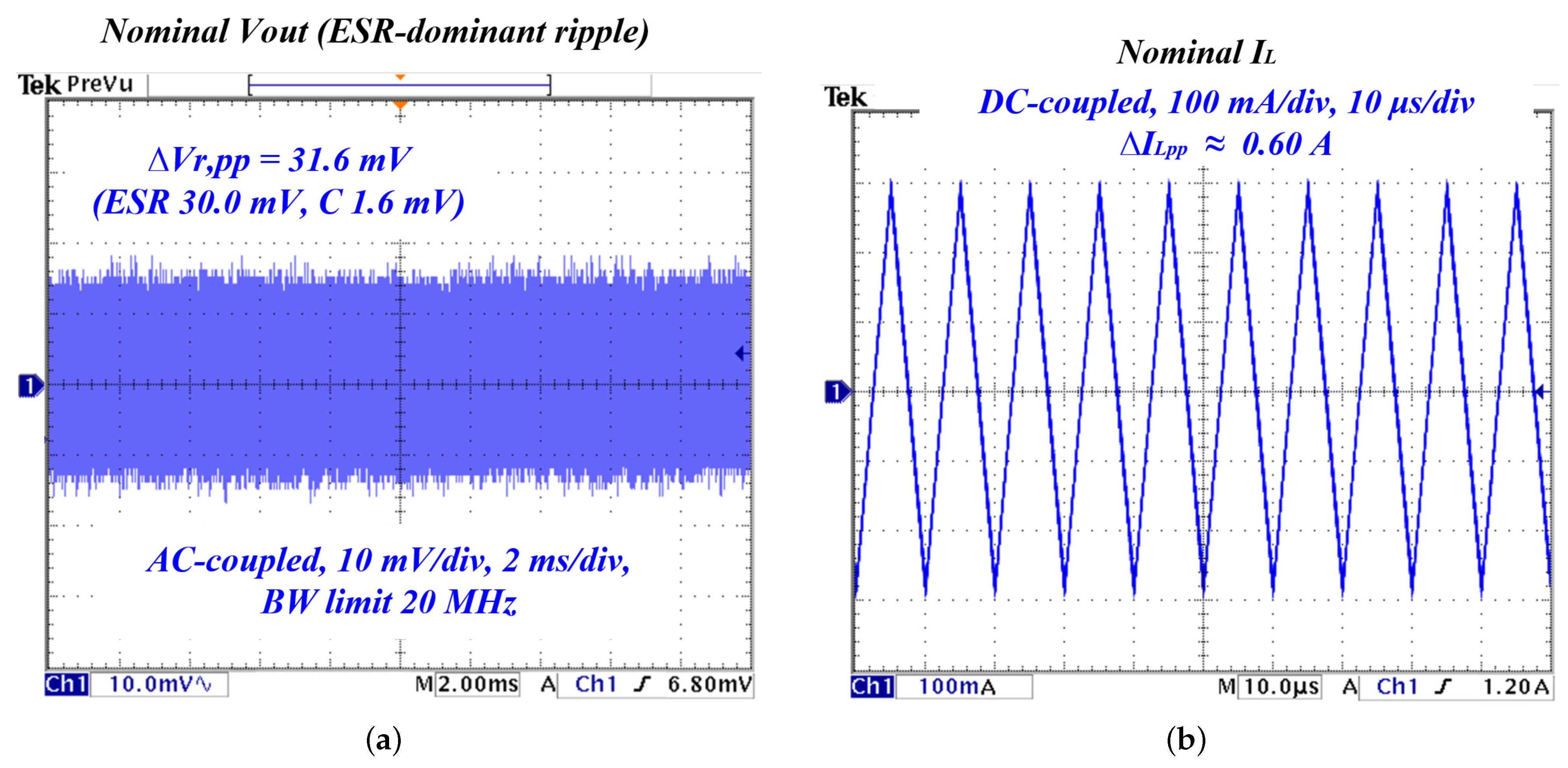
The output ripple is ESR-dominant. With Δ i L 0.60 A p p , C = 470 µ F , and f sw = 100 kHz , the ideal capacitive ripple is
Δ v C , p p Δ i L 8 C f sw 1.6 mV p p ,
whereas the ESR contribution is
Δ v ESR , p p Δ i L · ESR 0.60 × 0.05 = 30 mV p p .
The measured v o ripple (≈30 mV p p ) therefore matches the ESR estimate.

4.4.1. Baseline Operation

Figure 11 summarizes nominal buck operation. Figure 11a shows the output voltage ripple v o under 24 12 V, L = 100 µ H , C = 470 µ F , and f sw = 100 kHz . The measured ripple is ≈30 mV p p and is predominantly ESR-dominated: Δ v ESR , p p Δ i L ESR with Δ i L 0.60 A p p and ESR 50 m Ω ; the ideal capacitive component is small (≈1.6 mV p p ). Figure 11b shows the inductor current i L with DC 1.20 A and triangular ripple Δ i L 0.60 A p p governed by ( V i n , V o u t , D , L , f sw ) (e.g., D V o u t / V i n = 0.5 yields Δ i L ( V i n V o u t ) D / ( L f sw ) = 0.60 A p p ).
Consistency check. The reported values are cross-checked against first-principles estimates (Table 20).

4.4.2. Bias Injection

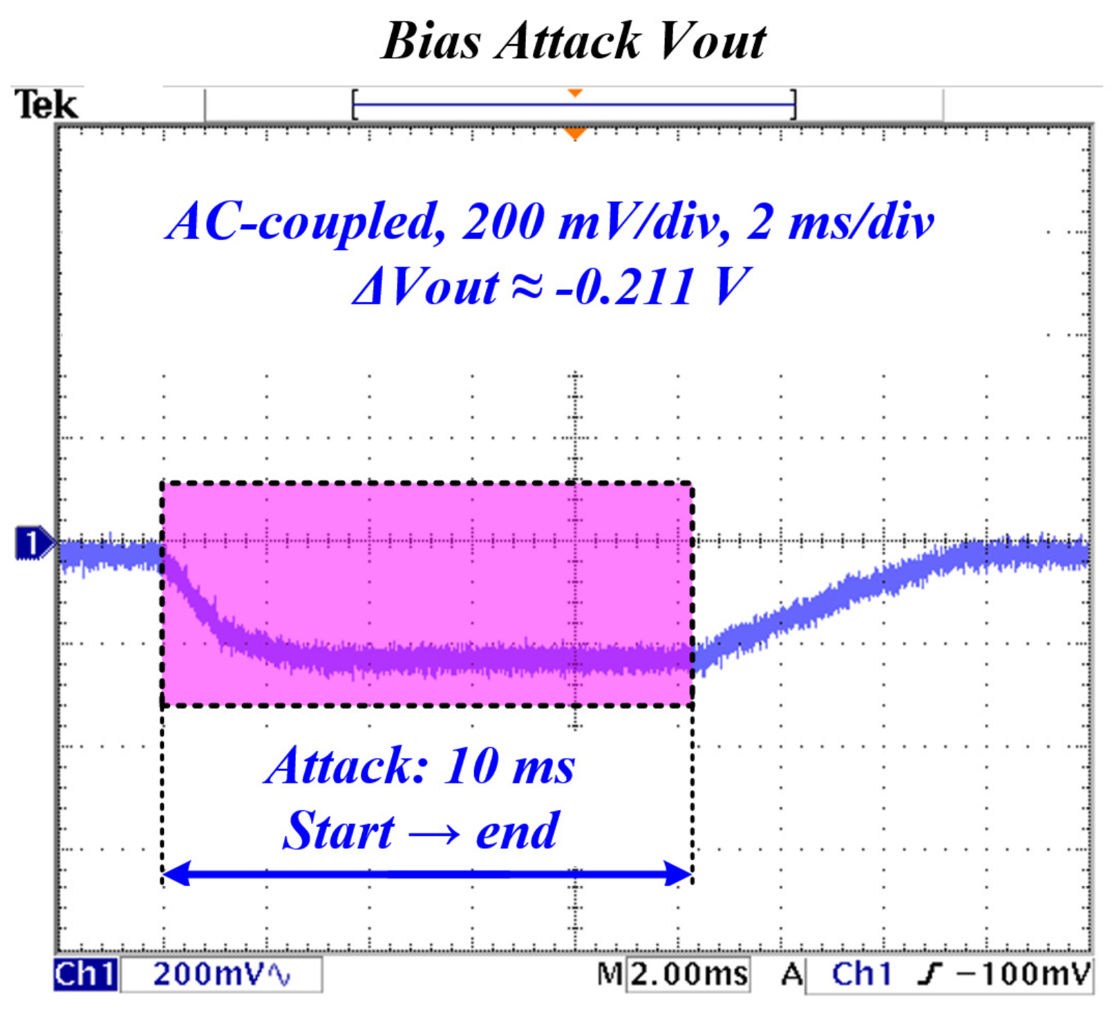
Figure 12 shows the output voltage with the attack window (50–70 ms) shaded. A + 0.4 V command yields an effective offset at the feedback node of δ eff + 58 mV (with divider ratio α 0.275 ). Under integral control without saturation, the steady-state shift follows Δ V out δ eff / α (see Equation (20)), matching the observed 0.21 V. After the attack ends, V out recovers to nominal within ∼8 ms. Scope settings: DC-coupled, 200 mV/div, 2 ms/div (10 divisions = 20 ms). Under the fixed decision rule ( τ = μ + 3 σ , N = 3 consecutive samples), the measured detection latency is 3.1 ms with an alarm-wise FPR of 0.8 % . We omit the inductor current trace here because its information (duty reduction and a small DC shift) is redundant with the voltage result; a current plot is included only for the delay case.

4.4.3. Delay Injection

Implementation. A fixed pure delay is inserted in the ADC DMA ISR PI path via a ring buffer of length N = 102 at f s = 100 kHz , giving τ = N / f s 1.02 ms (≈100 T s with T s = 10 µs). Scope-based step-to-actuation timing confirms that τ meas = 1.02 ± 0.03 ms ( n = 10 ).
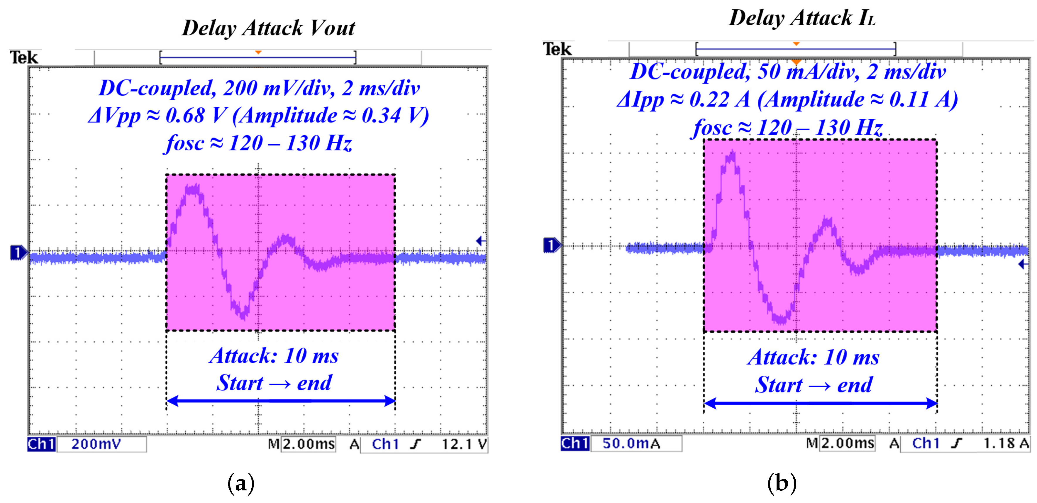
Figure 13a shows the output voltage with the attack window (50–70 ms) shaded. The additional phase lag ϕ delay ( f ) = 2 π f τ reduces the phase margin and produces a dominant ∼120–130 Hz component; the waveform returns to nominal after the attack ends. Figure 13b shows the inductor current; the same τ 1.02 ms introduces low-frequency modulation consistent with Figure 13a. Measured amplitudes: V out 0.34 V (amplitude; ≈0.68 V p p ) and i L 0.11 A (amplitude; ≈0.22 A p p ). Detection latency is 4.2 ms with alarm-wise FPR 1.2 % .
Origin > noindention here should be retained of the ∼120–130 Hz oscillation under delay.
The injected delay multiplies the nominal loop by e s τ , adding phase lag ϕ delay ( f ) = 360 f τ (deg) and reducing the effective phase margin to PM ( f ) PM 0 360 f τ . Zero-margin oscillation thus occurs near
f osc PM 0 360 τ .
With τ = 1.02 ms and a typical buck voltage loop margin PM 0 45 , f osc 123 Hz, matching the observed 120–130 Hz peak. The LC pole f 0 = ( 2 π L C ) 1 734 Hz ( L = 100 µH, C = 470 µF) is well above this; the modulation is due to phase margin erasure by delay, not LC resonance.
The reason that we include i L only for the delay case.
A fixed sensor path delay multiplies the loop by e s τ and reduces the phase margin (Equation (23)), producing a distinct low-frequency component (∼120–130 Hz) that is useful to show in both v o u t and i L . In contrast, for bias and 1 kHz noise injections, the i L trace is largely redundant with v o u t (similar shape with a small phase shift), so we omit i L there for brevity.

4.4.4. Noise Injection

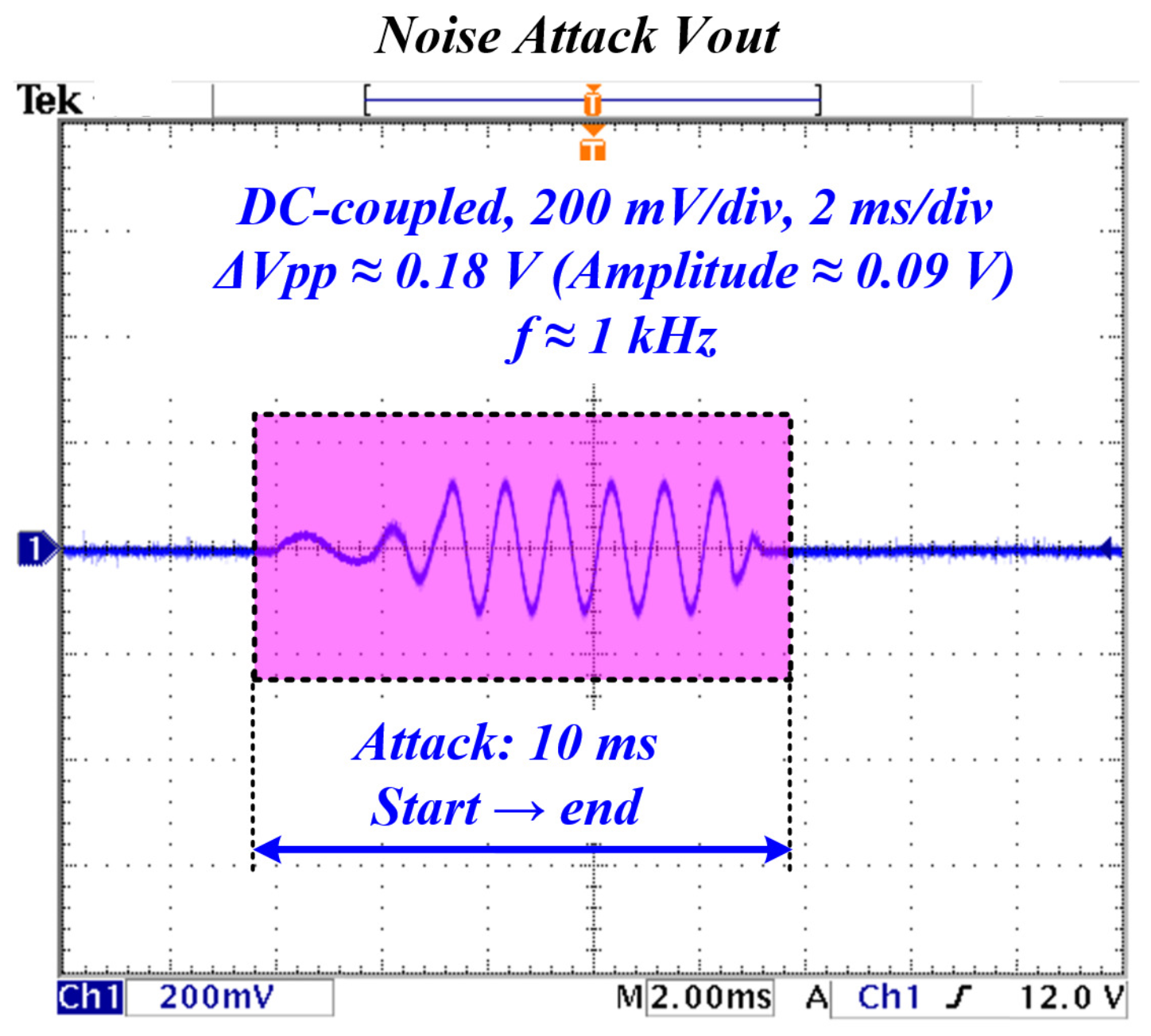
Figure 14 shows the output voltage with the attack window (50–70 ms) shaded. A 1 kHz sinusoid superimposed in the sensor path passes the closed loop with attenuation, leaving a distinct component of approximately 0.18 V p p (≈0.09 V amplitude) visible throughout the 20 ms window (about 20 cycles at 1 kHz). The nominal high-frequency switching ripple (∼30 mV p p ) remains superposed. Scope settings: DC-coupled, 200 mV/div, 2 ms/div (10 divisions = 20 ms). Under the fixed decision rule ( τ = μ + 3 σ , N = 3 consecutive samples), the measured detection latency is 2.9 ms with an alarm-wise FPR of 0.6 % . We omit the inductor current trace for this scenario because its small 1 kHz component is redundant with the voltage result; a single current plot is included only for the delay case.

4.4.5. Anomaly Score and Detection Performance

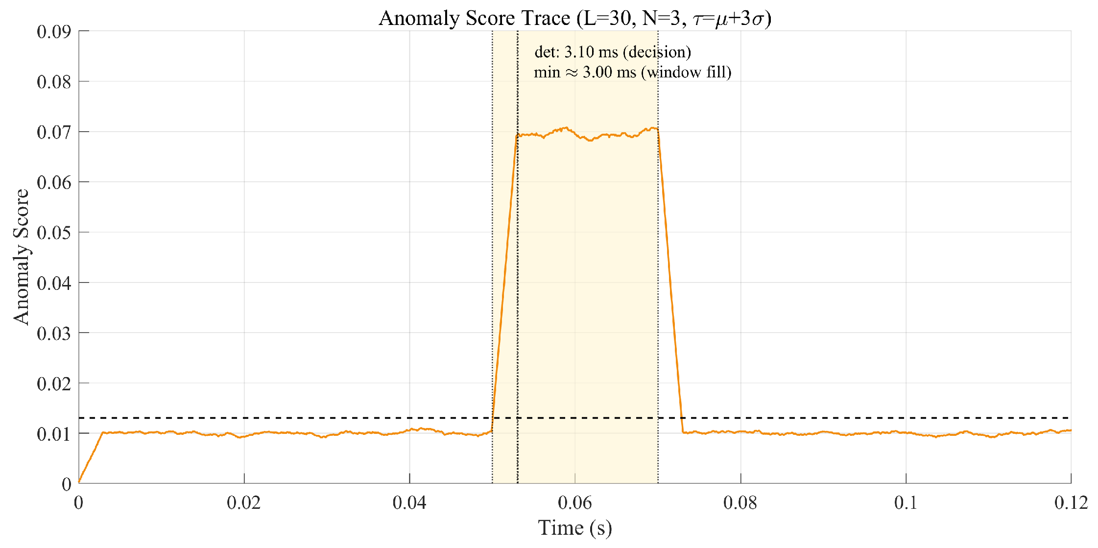
Figure 15 shows the hardware anomaly score trace replotted in MATLAB. A streaming PI–LSTM runs on a TMS320F28379 with inference rate f inf = 10 kHz (decimation M = 10 ), window L = 30 (3.0 ms), and an N = 3 consecutive-samples decision rule. The threshold is fixed at τ = μ + 3 σ from benign validation segments; the attack window (50–70 ms) is shaded.
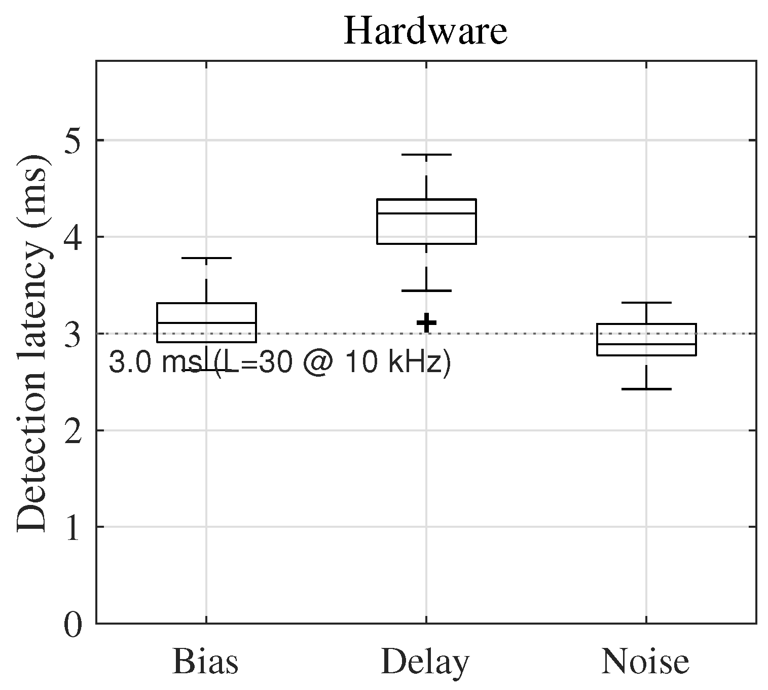
Figure 16 shows that the median detection latency is ordered as noise < bias < delay, with tight IQRs over n = 40 runs. The dotted 3.0 ms line (window span at f inf = 10 kHz, L = 30 ) provides context for the N = 3 persistence; the results are consistent with the simulation ordering (cf. Table 8) and with the fixed decision rule in Section 4.3.

4.4.6. Hardware Results with Confidence Intervals

We report hardware uncertainty using the conventions in Section 4.3: (i) latencies as the median with IQR and a bootstrap 95% confidence interval (B = 1000), (ii) the alarm-wise FPR as a point estimate with a Wilson score 95% interval. A campaign used n = 40 trials per attack (counts and intervals can be updated if a different n is used in the final campaign).
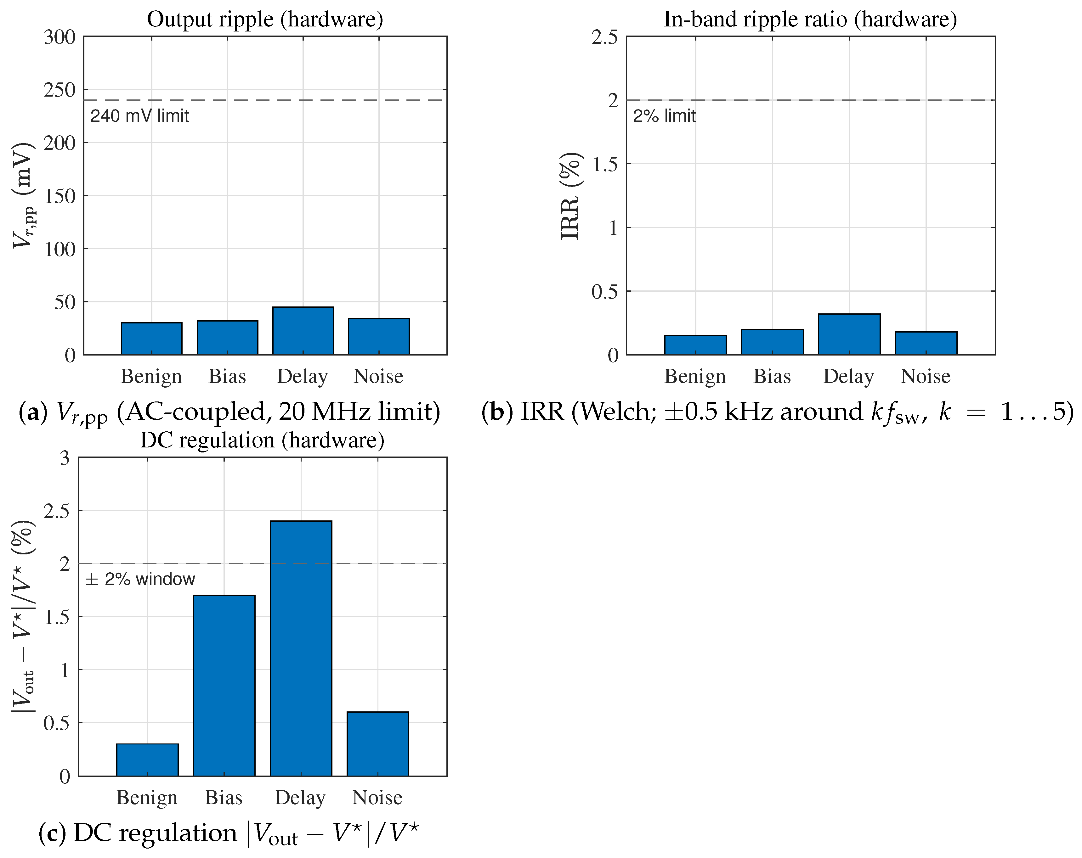
Figure 17 aggregates hardware measurements of V r , pp , the IRR , and the DC regulation error under benign/attack conditions. Across attacks, V r , pp and the IRR remain within their limits (see Equation (6)), while the ± 2 % regulation window is occasionally exceeded only for the delay case (peak 2.8 % ; Section 4.3), matching the score/latency behavior and the delay-induced phase margin erosion discussed earlier.
Hardware detection metrics with 95% confidence intervals are summarized in Table 21.
Under this rule, the anomaly score exceeds the threshold with low latency:
  • Bias: latency 3.1 ms; FPR 0.8 % ;
  • Delay: latency 4.2 ms; FPR 1.2 % ;
  • Noise: latency 2.9 ms; FPR 0.6 % .
These hardware results follow the simulation trends in relative difficulty and latency. The time-domain ripple V r , p p and IRR remained within the limits, whereas the delay attack produced a low-frequency deviation up to ≈0.34 V (≈2.8%), which could exceed the ± 2 % regulation window. CI-guided actuation (which enforces the full safety box) was evaluated in the simulation only.
Safety compliance summary. In the hardware experiments without CI-based actuation, (i) the V r , p p and IRR satisfied their limits; (ii) the ± 2 % DC regulation window was occasionally exceeded under the delay attack (peak 2.8 % ). With CI-based actuation (simulation study), all three constraints were satisfied concurrently. A concise summary is given in Table 22.
Claim scope and robustness safeguards. We emphasize that our deployability claim refers to the detection path; CI-guided actuation has been evaluated in simulations only. The occasional violation of the ± 2 % regulation window under the delay attack (peak 2.8 % ) motivated two firmware safeguards that gate actuation: (i) a regulation/ripple watchdog that rolls back to α = 0 when any metric exceeds 90 % of its limit (i.e., | V out V | / V > 1.8 % , V r , pp > 0.9 · 240 mV , IRR > 0.9 · 2 % ); (ii) a delay-aware guard that monitors the 100 150 Hz band (Goertzel) and suppresses actuation when the component exceeds a calibrated threshold, consistent with the phase margin erosion observed under a fixed sensor path delay. These safeguards are designed to keep regulation within bounds during CI actuation; their hardware validation is included in the future work test matrix and acceptance criteria.
Scope note. Hardware CI-guided actuation and richer threat models are outside the scope of this paper and are enumerated in Future Workwith acceptance criteria; the present deployability claim pertains to the detection path.
Scope and generalizability. This hardware study intentionally focuses on a buck converter and three sensor-side disturbances (bias, fixed sample delay, narrowband noise) to validate the detection path and safety box instrumentation end-to-end on a DSP with reproducible latency/FPR. The PI–LSTM formulation itself is topology-agnostic: the physics loss enforces discrete-time state updates, so replacing the buck update map with that of another topology yields a drop-in variant.
Residual template. For any averaged DC–DC topology with fixed-step update x k + 1 = f d ( x k , u k ; θ ) at sampling period Δ t ,
L phys = 1 N b k = 1 N b x ^ k + 1 f d x ^ k , u ^ k ; θ 2 2
where x collects topology states (e.g., [ i L , v o ] for buck; [ i L , v C ] for boost/buck–boost), and u includes duty d (and, if needed, phase indices for multiphase VRM). Multiphase extensions add phase balance/residual terms (e.g., p i L , p i L = 0 or ripple constraints).
Threat model extensions (planned). Actuator path tampering (duty/PWM saturation), time-varying delay/jitter, load-side steps/sags, supply sags/surges, wideband EMI/harness coupling, and network-level MITM leading to sensor path anomalies. The Future Work section specifies a test matrix and acceptance criteria for these scenarios and for boost, buck–boost, and multiphase VRM.

4.4.7. CI-Based Actuation: Hardware Implementation Plan

We outline a phased plan to deploy CI-guided actuation on the DSP while enforcing the unified safety box V r , pp 240 mV , IRR 2 % , | V out V | / V 2 % .
(A) Architecture and hook points. The CI is computed at the inference rate ( f inf = 10 kHz, window L = 30 , persistence N = 3 , T hys = 10 ms). The actuation channels are { V ref , d , f sw } with α [ 0 , α max ] ( α max = 0.35 ), gains ( k v , k d , k f ) = ( 0.04 , 0.03 , 0.05 ) , and rate limiters (per-tick | Δ V ref | , | Δ d | , | Δ f sw | bounded). Hard clamps ensure PWM duty in [ d min , d max ] and f sw in [ f min , f max ] . Any limit approach (≥90% of the bound) reduces α (rollback) and restores nominal setpoints.
(B) On-board estimators for CI terms. Ripple (time):  V r , pp from an AC-coupled trace via a sliding window spanning 5–10 switching periods (peak-to-peak over detrended samples). Ripple (freq):  IRR via narrowband power around k f sw ( k = 1 5 ): compute RMS using Goertzel/IIR band-pass pairs with ± 0.5 kHz equivalent bandwidth; normalize by V out , DC . Efficiency:  η P out / P in using available voltage/current sensors ( V out , I out , V in , I in ); when a current is unavailable, use a calibrated proxy (e.g., P out V out · I L in CCM with shunt/Hall scaling).
(C) Safety interlocks and supervision. (1) Dual-threshold gating: detection ( τ = μ + 3 σ , N = 3 ) must persist for T hys before actuation; (2) watchdog (e.g., 2 ms) on the CI task; timeout ⇒ restore nominal; (3) hardware kill-switch and firmware latch to freeze α = 0 ; (4) thermal/overcurrent monitors ( T j , I L rms ) inhibit actuation.
(D) Commissioning phases (with logging at 1 kHz). P0 HIL/SIL: verify estimators and α logic off-target; P1 passive logging (no actuation); P2 shadow mode: compute α but do not apply, check rollback triggers and safety margins; P3 limited actuation: apply V ref and d only, α max 0.20 , no f sw change; P4 extended actuation: enable f sw adjustment with tight clamps, α max 0.35 .
(E) Test matrix and acceptance criteria. Attacks: bias, delay (≈1.02 ms), narrowband noise (∼1 kHz); loads: nominal ±20%, line ±10%. Pass if, under CI actuation, (i) no violation of any limit; (ii) median detection latency within prior ranges (∼2.9–4.2 ms); (iii) alarm-wise FPR within prior ranges (≤1.2%); (iv) automatic rollback engaged when any metric exceeds 90% of limit; (v) no watchdog timeouts or safety latches during steady operation.
(F) Runtime and footprint. CI updates reuse the existing 10 kHz loop. The added cost of K = 5 Goertzel filters per channel is within the DSP margin (<15% extra CPU in our budget), keeping the total load <70% at 200 MHz. All settings are logged (UART/SD) for audit.

4.4.8. Limitations and Robustness Considerations

Temperature and component drift. ESR(C), L, divider ratio α fb , and sensor/ADC offsets drift with temperature and aging, which can shift the loop gain and V r , pp / IRR . Our fixed threshold ( τ = μ + 3 σ from room-temperature benign data) may become suboptimal under large ambient excursions. Mitigation: Periodic benign recalibration (mean/variance refresh), temperature-tagged normalization, and scheduled verification across operating corners.
EMI and sensing chain. Unmodeled narrowband/broadband EMI, grounding/harness coupling, and probe/anti-alias choices affect the sensed channels. Because the IRR integrates only around k f sw , off-band tones (e.g., ∼1 kHz ) primarily impact regulation and V r , pp rather than the IRR ; conversely, near- k f sw EMI can inflate the IRR . Mitigation: Differential sensing, twisted/shielded lines, RC anti-aliasing before the ADC, and notch/band limit where allowed.
Modeling gap in PI loss. The physics residuals use an averaged discrete-time buck model and omit switch-level nonidealities (dead time, frequency-dependent ESR, diode reverse recovery). Under a large ripple or discontinuous operation, residual penalties may be imperfect. Mitigation: Extend residuals with collocation/regularization or hybrid terms identified from measured data.
Inference rate/latency trade-off. Deployment uses f inf = 10 kHz with L = 30 (≈3.0 ms ) and N = 3 , setting a latency floor of a few milliseconds and limiting sub-ms detection. Mitigation: Reduce decimation or L within the DSP budget; exploit quantization or fused kernels to maintain the load.
Fixed global decision rule. A single global τ is robust but can be conservative under fast load/operating point changes. Mitigation: Per-mode thresholds or guarded online updates (e.g., percentile tracking on verified benign segments).
Scope of actuation. CI-guided actuation was evaluated in simulations only; hardware validation covered the detection path. Safety box satisfaction on hardware under closed-loop CI actuation remains for future work.
Measurement uncertainty. Ripple is AC-coupled (20 MHz limit) and IRR is computed by Welch integration; probe/setup choices introduce uncertainty. We therefore report medians/IQRs and 95% intervals for hardware metrics.
Scope of claims. All conclusions on the DC rail quality, the unified safety box, and CI-guided actuation pertain to the buck converter domain. The PMSM dataset is used solely for an auxiliary, cross-domain test after the alignment in Section 3.2; we report detection metrics only and do not compute or interpret DC rail ripple metrics for this dataset.

5. Conclusions

We presented a physics-informed anomaly detector for digitally controlled DC–DC converters that couples an LSTM autoencoder with discrete-time circuit residuals and a unified safety box for DC regulation ( ± 2 % ), time-domain ripple V r , pp , and the in-band ripple ratio (IRR).
Simulation. Across bias, delay, and narrowband noise attacks, the PI–LSTM improved the average F1 by ∼6.6% (89.3→95.2%), reduced the alarm-wise FPR by ∼53% (12.4→5.8%), and lowered the physical violation rate by ∼86% versus a conventional LSTM. A safety-bounded CI response achieved a CI 0.25 while remaining within limits.
Hardware. On a TMS320F28379, a distilled ( n x = 4 , n h = 32 ) model achieved 2.9–4.2 ms latency with alarm-wise FPR 1.2 % . Ripple metrics ( V r , pp , IRR) met limits; under delay, the ± 2 % regulation window was occasionally exceeded (peak 2.8 % ). Deployability here pertains to the detection path; CI-based actuation remains simulation-only.
Industrial/commercial note. The detector runs as a drop-in library on common MCU/DSP targets (e.g., C28x, ARM-M4/M7). Target segments include EV on-board DC–DC/chargers, PV DC-link, ESS, and industrial SMPS/UPS. Optional edge–gateway–cloud integration supports fleet analytics/OTA, while local safety is enforced by the unified safety box.
Future work.
  • HIL/on-rig CI actuation under the unified safety box. Close the loop on HIL and hardware for CI-guided actuation while enforcing the same limits used in this paper: | V out V | / V ± 2 % , V r , pp 240 mV , IRR 2 % . Acceptance targets: median detection latency within the prior 2.9–4.2 ms band; alarm-wise FPR 1.2 % ; zero safety box violations during CI engagement with rollback/hysteresis enabled.
  • Threat model and topology expansion. Evaluate more complex disturbances (multi-tone/near- k f sw EMI, sampled data jitter/delay spread, ADC range/quantization effects, sensor drift + load steps) and extend the residual template to boost, buck–boost, and multiphase VRM with optional multi-sensor fusion.
  • System-level performance and resilience across environments. Quantify efficiency drop and energy overhead, delay-sensitive oscillation proxies, and fleet indicators (alarm density, MTTR, score drift index) across temperature/aging (e.g., 20 85 ° C), ESR/inductance drift, and EMI injection; retain the fixed decision policy ( τ = μ + 3 σ , N = 3 ) with periodic benign rethresholding.
  • Distributed integration (edge–gateway–cloud). Keep safety local on the controller (fail closed to α = 0 ). Gateway aggregates 1–5 Hz summaries (OPC UA/MQTT/TLS), supports OTA with versioning/rollback; cloud performs drift monitoring and replay-based validation. Budgets: <0.1 ms/step at 10 kHz inference; ∼0.2–2.5 kB/s telemetry per node.
  • Commercialization pilots. Run pilots in two–three domains (EV on-board DC–DC/charger, PV DC-link, ESS) to assess readiness. Targets: latency band preserved (median report), FPR 1.2 % , no safety box violations, and reduced nuisance trips vs. baseline. Deliverables: firmware library (porting guide), add-on module reference design, gateway/OTA workflows (audit logs, rollback).
  • Industrial practice readiness. Prepare lightweight hardening and pre-compliance—QA test pack (temperature, aging, ESR and inductance (L) drift, EMI)—documentation for integration and O&M (commissioning: logging → shadow mode → gated actuation)—and pre-assess applicable standards (e.g., IEC 61204-3 [55], IEC 62443-2-1 [61], ISO 26262 [62], ISO/SAE 21434 [63]).
  • Adaptive operations (optional). Operating mode-aware thresholds and change point detection while retaining the N = 3 persistence policy; quantization/pruning for sub-40 µs/step at 200 MHz without loss of detection performance.
Reproducibility. A curated package (code/data/models/figure scripts and hardware logs) will be released on Zenodo upon acceptance and/or institutional clearance; the auxiliary PMSM dataset is public (Ref. [39]).

Supplementary Materials

The following supporting information can be downloaded at: https://www.mdpi.com/article/10.3390/app152011112/s1. File S1. Statistical reporting conventions; File S2. Derivations and decision rules; File S3. Confusion index (CI) weighting sensitivity; File S4. Reproducibility artifacts.

Author Contributions

Conceptualization, J.-H.M. and J.-H.L.; methodology, J.-H.L. and J.-H.K.; software, J.-H.K. and J.-H.M.; validation, J.-H.M., J.-H.L. and J.-H.K.; formal analysis, J.-H.K. and J.-H.M.; investigation, J.-H.M. and J.-H.K.; data curation, J.-H.M., J.-H.L. and J.-H.K.; writing—original draft preparation, J.-H.M.; writing—review and editing, J.-H.M. and J.-H.L.; funding acquisition, J.-H.L.; project administration, J.-H.M. and J.-H.L. All authors have read and agreed to the published version of the manuscript.

Funding

This work was supported by the Research Fund from Honam University in 2023.

Data Availability Statement

The data supporting the findings of this study are available from the corresponding author upon reasonable request. A curated reproducibility package (simulation data, trained models, figure scripts, and hardware logs) will be made publicly available on Zenodo (Version 1.0) upon acceptance and/or institutional clearance. The auxiliary PMSM dataset is publicly available on Zenodo; see Ref. [39].

Conflicts of Interest

The authors declare no conflicts of interest.

Abbreviations

ADCAnalog-to-Digital Converter
AEAutoencoder
CCMContinuous Conduction Mode
CIConfusion Index (not a statistical confidence interval)
DSPDigital Signal Processor
DSODigital Storage Oscilloscope
ESR         Equivalent Series Resistance
HILHardware-in-the-Loop
IRRIn-Band Ripple Ratio
LSTMLong Short-Term Memory
PI–LSTMPhysics-Informed LSTM
PSDPower Spectral Density
PWMPulse Width Modulation

References

  1. Mazumder, S.K.; Kulkarni, A.; Sahoo, S.; Blaabjerg, F.; Mantooth, H.A.; Balda, J.C.; Zhao, Y.; Ramos-Ruiz, J.A.; Enjeti, P.N.; Kumar, P.; et al. A review of current research trends in power-electronic innovations in cyber–physical systems. IEEE J. Emerg. Sel. Top. Power Electron. 2021, 9, 5146–5163. [Google Scholar] [CrossRef]
  2. Parizad, A.; Baghaee, H.R.; Alizadeh, V.; Rahman, S. Emerging Technologies and Future Trends in Cyber-Physical Power Systems: Toward a New Era of Innovations. Smart-Cyber-Phys. Power Syst. Solut. Emerg. Technol. 2025, 2, 525–565. [Google Scholar]
  3. Chukwunweike, J.N.; Agosa, A.A.; Mba, U.J.; Okusi, O.; Safo, N.O.; Onosetale, O. Enhancing Cybersecurity in Onboard Charging Systems of Electric Vehicles: A MATLAB-based Approach. World J. Adv. Res. Rev. 2024, 23, 2661–2681. [Google Scholar] [CrossRef]
  4. Arena, G.; Chub, A.; Lukianov, M.; Strzelecki, R.; Vinnikov, D.; De Carne, G. A comprehensive review on DC fast charging stations for electric vehicles: Standards, power conversion technologies, architectures, energy management, and cybersecurity. IEEE Open J. Power Electron. 2024, 5, 1573–1611. [Google Scholar] [CrossRef]
  5. Yu, X.; Wang, H.; Dong, K.; Chen, C. A novel LDVP-based anomaly detection method for data streams. Int. J. Comput. Appl. 2024, 46, 381–389. [Google Scholar] [CrossRef]
  6. Tabassum, T.; Toker, O.; Khalghani, M.R. Cyber–physical anomaly detection for inverter-based microgrid using autoencoder neural network. Appl. Energy 2024, 355, 122283. [Google Scholar] [CrossRef]
  7. Hwang, S.Y.; Lee, J.c.; Lee, S.s.; Min, C. Anomaly-Detection Framework for Thrust Bearings in OWC WECs Using a Feature-Based Autoencoder. J. Mar. Sci. Eng. 2025, 13, 1638. [Google Scholar] [CrossRef]
  8. Alserhani, F. Intrusion Detection and Real-Time Adaptive Security in Medical IoT Using a Cyber-Physical System Design. Sensors 2025, 25, 4720. [Google Scholar] [CrossRef]
  9. Mahmoudi, I.; Boubiche, D.E.; Athmani, S.; Toral-Cruz, H.; Chan-Puc, F.I. Toward Generative AI-Based Intrusion Detection Systems for the Internet of Vehicles (IoV). Future Int. 2025, 17, 310. [Google Scholar] [CrossRef]
  10. Santoso, A.; Surya, Y. Maximizing decision efficiency with edge-based AI systems: Advanced strategies for real-time processing, scalability, and autonomous intelligence in distributed environments. Q. J. Emerg. Technol. Innov. 2024, 9, 104–132. [Google Scholar]
  11. Ottaviano, D. Real-Time Virtualization of Mixed-Criticality Heterogeneous Embedded Systems for Fusion Diagnostics and Control. 2025. Available online: https://www.research.unipd.it/handle/11577/3552539 (accessed on 23 September 2025).
  12. Isermann, R. Fault-Diagnosis Systems: An Introduction from Fault Detection to Fault Tolerance; Springer: Berlin/Heidelberg, Germany, 2006. [Google Scholar]
  13. Givi, H.; Farjah, E.; Ghanbari, T. A Comprehensive Monitoring System for Online Fault Diagnosis and Aging Detection of Non-Isolated DC–DC Converters’ Components. IEEE Trans. Power Electron. 2019, 34, 6858–6875. [Google Scholar] [CrossRef]
  14. Geddam, K.K.; Elangovan, D. Review on fault-diagnosis and fault-tolerance for DC–DC converters. IET Power Electron. 2020, 13, 3071–3086. [Google Scholar]
  15. Raissi, M.; Perdikaris, P.; Karniadakis, G.E. Physics-informed neural networks: A deep learning framework for solving forward and inverse problems involving nonlinear partial differential equations. J. Comput. Phys. 2019, 378, 686–707. [Google Scholar] [CrossRef]
  16. Karniadakis, G.E.; Kevrekidis, I.G.; Lu, L.; Perdikaris, P.; Wang, S.; Yang, L. Physics-informed machine learning. Nat. Rev. Phys. 2021, 3, 422–440. [Google Scholar] [CrossRef]
  17. Lu, L.; Meng, X.; Mao, Z.; Karniadakis, G.E. DeepXDE: A deep learning library for solving differential equations. SIAM Rev. 2021, 63, 208–228. [Google Scholar] [CrossRef]
  18. Cuomo, S.; Di Cola, V.; Giampaolo, F.; Rozza, G.; Raissi, M.; Piccialli, F. Scientific Machine Learning Through Physics-Informed Neural Networks: Where we are and What’s next. J. Sci. Comput. 2022, 92, 88. [Google Scholar] [CrossRef]
  19. Raissi, M.; Yazdani, A.; Karniadakis, G.E. Hidden fluid mechanics: Learning velocity and pressure fields from scalar concentration only. Science 2020, 367, 1026–1030. [Google Scholar] [CrossRef] [PubMed]
  20. Karpatne, A.; Atluri, G.; Faghmous, J.H.; Steinbach, M.; Banerjee, A.; Ganguly, A.R.; Shekhar, S.; Samatova, N.; Kumar, V. Theory-Guided Data Science: A New Paradigm for Scientific Discovery from Data. IEEE Trans. Knowl. Data Eng. 2017, 29, 2318–2331. [Google Scholar] [CrossRef]
  21. Yang, S.; Bryant, A.; Mawby, P.; Xiang, D.; Ran, L.; Tavner, P. Condition Monitoring for Device Reliability in Power Electronic Converters: A Review. IEEE Trans. Power Electron. 2010, 25, 2734–2752. [Google Scholar] [CrossRef]
  22. Buiatti, G.M.; Martín-Ramos, J.A.; Rojas García, C.H.; Amaral, A.M.R.; Cardoso, A.J.M. An Online and Noninvasive Technique for the Condition Monitoring of Capacitors in Boost Converters. IEEE Trans. Instrum. Meas. 2010, 59, 2134–2143. [Google Scholar] [CrossRef]
  23. Elabid, Z. Informed Deep Learning for Modeling Physical Dynamics. Ph.D. Thesis, Sorbonne Université, Paris, France, 2025. [Google Scholar]
  24. Mansuri, A.; Maurya, R.; Suhel, S.M.; Iqbal, A. Random Switching Pulse Positioning based SVM Techniques for Six-Phase AC Drive to Spread Harmonic Spectrum. IEEE J. Emerg. Sel. Top. Power Electron. 2025, 13, 6531–6540. [Google Scholar] [CrossRef]
  25. Ekin, Ö.; Perez, F.; Wiegel, F.; Hagenmeyer, V.; Damm, G. Grid supporting nonlinear control for AC-coupled DC Microgrids. In Proceedings of the 2024 IEEE Sixth International Conference on DC Microgrids (ICDCM), Columbia, SC, USA, 5–8 August 2024; IEEE: New York, NY, USA, 2024; pp. 1–6. [Google Scholar]
  26. Ulrich, B. A low-cost setup and procedure for measuring losses in inductors. In Proceedings of the 2025 IEEE Applied Power Electronics Conference and Exposition (APEC), Atlanta, GA, USA, 16–20 March 2025; IEEE: New York, NY, USA, 2025; pp. 2502–2509. [Google Scholar]
  27. Bolatbek, Z. Single Shot Spectroscopy Using Supercontinuum and White Light Sources; University of Dayton: Dayton, OH, USA, 2024. [Google Scholar]
  28. Kim, H.; Bandyopadhyay, R.; Ozmen, M.O.; Celik, Z.B.; Bianchi, A.; Kim, Y.; Xu, D. A systematic study of physical sensor attack hardness. In Proceedings of the 2024 IEEE Symposium on Security and Privacy (SP), San Francisco, CA, USA, 20–22 May 2024; IEEE: New York, NY, USA, 2024; pp. 2328–2347. [Google Scholar]
  29. Lian, Z.; Shi, P.; Chen, M. A Survey on Cyber-Attacks for Cyber-Physical Systems: Modeling, Defense and Design. IEEE Int. Things J. 2024, 12, 1471–1483. [Google Scholar] [CrossRef]
  30. Cao, H.; Huang, W.; Xu, G.; Chen, X.; He, Z.; Hu, J.; Jiang, H.; Fang, Y. Security analysis of WiFi-based sensing systems: Threats from perturbation attacks. arXiv 2024, arXiv:2404.15587. [Google Scholar]
  31. Jiang, D.; Zhang, M.; Xu, Y.; Qian, H.; Yang, Y.; Zhang, D.; Liu, Q. Rotor dynamic response prediction using physics-informed multi-LSTM networks. Aerosp. Sci. Technol. 2024, 155, 109648. [Google Scholar] [CrossRef]
  32. Atila, H.; Spence, S.M. Metamodeling of the response trajectories of nonlinear stochastic dynamic systems using physics-informed LSTM networks. J. Build. Eng. 2025, 111, 113447. [Google Scholar] [CrossRef]
  33. Ma, Z.; Jiang, G.; Chen, J. Physics-informed ensemble learning with residual modeling for enhanced building energy prediction. Energy Build. 2024, 323, 114853. [Google Scholar] [CrossRef]
  34. Wang, Y.; Sun, J.; Bai, J.; Anitescu, C.; Eshaghi, M.S.; Zhuang, X.; Rabczuk, T.; Liu, Y. Kolmogorov–Arnold-Informed neural network: A physics-informed deep learning framework for solving forward and inverse problems based on Kolmogorov–Arnold Networks. Comput. Methods Appl. Mech. Eng. 2025, 433, 117518. [Google Scholar] [CrossRef]
  35. Fu, B.; Gao, Y.; Wang, W. A physics-informed deep reinforcement learning framework for autonomous steel frame structure design. Comput.-Aided Civ. Infrastruct. Eng. 2024, 39, 3125–3144. [Google Scholar] [CrossRef]
  36. Bagheri, A.; Patrignani, A.; Ghanbarian, B.; Pourkargar, D.B. A hybrid time series and physics-informed machine learning framework to predict soil water content. Eng. Appl. Artif. Intell. 2025, 144, 110105. [Google Scholar] [CrossRef]
  37. Nguyen, M.H.; Kwak, S.; Choi, S. Model Predictive Virtual Flux Control Method for Low Switching Loss Performance in Three-Phase AC/DC Pulse-width-Modulated Converters. Machines 2024, 12, 66. [Google Scholar] [CrossRef]
  38. Fedele, E.; Spina, I.; Di Noia, L.P.; Tricoli, P. Multi-Port Traction Converter for Hydrogen Rail Vehicles: A Comparative Study. IEEE Access 2024, 12, 174888–174900. [Google Scholar] [CrossRef]
  39. Bacha, A. Comprehensive Dataset for Fault Detection and Diagnosis in Inverter-Driven PMSM Systems (Version 3.0) [Data set]. Zenodo. 2024. Available online: https://www.sciencedirect.com/science/article/pii/S2352340925000186 (accessed on 8 October 2025).
  40. Shaheed, K.; Szczuko, P.; Kumar, M.; Qureshi, I.; Abbas, Q.; Ullah, I. Deep learning techniques for biometric security: A systematic review of presentation attack detection systems. Eng. Appl. Artif. Intell. 2024, 129, 107569. [Google Scholar] [CrossRef]
  41. Rajendran, R.M.; Vyas, B. Detecting apt using machine learning: Comparative performance analysis with proposed model. In Proceedings of the SoutheastCon 2024, Atlanta, GA, USA, 15–24 March 2024; IEEE: New York, NY, USA, 2024; pp. 1064–1069. [Google Scholar]
  42. Kim, H.G.; Park, Y. Calibrating F1 Scores for Fair Performance Comparison of Binary Classification Models with Application to Student Dropout Prediction. IEEE Access 2025, 13, 136554–136567. [Google Scholar] [CrossRef]
  43. Xu, T. Credit risk assessment using a combined approach of supervised and unsupervised learning. J. Comput. Methods Eng. Appl. 2024, 4, 1–12. [Google Scholar] [CrossRef]
  44. Khanmohammadi, F.; Azmi, R. Time-series anomaly detection in automated vehicles using d-cnn-lstm autoencoder. IEEE Trans. Intell. Transp. Syst. 2024, 25, 9296–9307. [Google Scholar] [CrossRef]
  45. Long, S.; Zhou, Q.; Ying, C.; Ma, L.; Luo, Y. Rethinking domain generalization: Discriminability and generalizability. IEEE Trans. Circuits Syst. Video Technol. 2024, 34, 11783–11797. [Google Scholar] [CrossRef]
  46. Jiang, F.; Li, Q.; Wang, W.; Ren, M.; Shen, W.; Liu, B.; Sun, Z. Open-set single-domain generalization for robust face anti-spoofing. Int. J. Comput. Vis. 2024, 132, 5151–5172. [Google Scholar] [CrossRef]
  47. Arpinati, L.; Carradori, G.; Scherz-Shouval, R. CAF-induced physical constraints controlling T cell state and localization in solid tumours. Nat. Rev. Cancer 2024, 24, 676–693. [Google Scholar] [CrossRef]
  48. Jiang, L.; Hu, Y.; Liu, Y.; Zhang, X.; Kang, G.; Kan, Q. Physics-informed machine learning for low-cycle fatigue life prediction of 316 stainless steels. Int. J. Fatigue 2024, 182, 108187. [Google Scholar] [CrossRef]
  49. Kwon, Y.; Kim, W.; Kim, H. HARD: Hardware-Aware lightweight Real-time semantic segmentation model Deployable from Edge to GPU. In Proceedings of the Asian Conference on Computer Vision, Hanoi, Vietnam, 8–12 December 2024; pp. 3552–3569. [Google Scholar]
  50. Gao, B.; Kong, X.; Li, S.; Chen, Y.; Zhang, X.; Liu, Z.; Lv, W. Enhancing anomaly detection accuracy and interpretability in low-quality and class imbalanced data: A comprehensive approach. Appl. Energy 2024, 353, 122157. [Google Scholar] [CrossRef]
  51. Instruments, T. The TMS320F2837xD Architecture: Achieving a New Level of High Performance. Technical Article SPRT720, Texas Instruments. 2016. Available online: https://www.radiolocman.com/datasheet/data.html?di=333939&/TMS320F28379D (accessed on 23 September 2025).
  52. Instruments, T. TMS320C28x Extended Instruction Sets Technical Reference Manual; Texas Instruments: Dallas, TX, USA, 2019. [Google Scholar]
  53. ISO 16750-2:2023; Road Vehicles—Environmental Conditions and Testing for Electrical and Electronic Equipment—Part 2: Electrical Loads. International Organization for Standardization: Geneva, Switzerland, 2023.
  54. ISO 21780:2020; Road Vehicles—Supply Voltage of 48 V—Electrical Requirements and Tests. International Organization for Standardization: Geneva, Switzerland, 2020.
  55. IEC 61204-3:2016; Low-Voltage Power Supplies, DC Output—Part 3: Electromagnetic Compatibility (EMC). International Electrotechnical Commission: Geneva, Switzerland, 2016.
  56. Single Rail Power Supply ATX12VO Design Guide. In Design Guide; Intel Corporation: Santa Clara, CA, USA, 2020.
  57. Power Supply Measurement and Analysis with Bench Oscilloscopes. In Technical Report Application Note 3GW-23612-6; Tektronix, Inc.: Beaverton, OR, USA, 2014.
  58. Instruments, T. Cycle Scavenging on C2000™ MCUs, Part 5: TMU and CLA. Technical Article. 2017. Available online: https://www.ti.com/lit/ta/sszt866/sszt866.pdf?ts=1760149313235&ref_url=https%253A%252F%252Fwww.google.com.hk%252F (accessed on 7 September 2025).
  59. Instruments, T. TMS320F2837xD Dual-Core Real-Time Microcontrollers Technical Reference Manual; Texas Instruments: Dallas, TX, USA, 2024. [Google Scholar]
  60. MathWorks. C28x-Build Options—Enable FastRTS. Online Documentation. 2025. Available online: https://www.mathworks.com/help/ti-c2000/ref/sect-hw-imp-pane-c28x-build-options.html (accessed on 7 September 2025).
  61. IEC 62443-2-1:2024; Security for Industrial Automation and Control Systems—Part 2-1: Security Program Requirements for IACS Asset Owners. International Electrotechnical Commission: Geneva, Switzerland, 2024.
  62. ISO 26262:2018; Road Vehicles—Functional Safety (All Parts). International Organization for Standardization: Geneva, Switzerland, 2018.
  63. ISO/SAE 21434:2021; Road Vehicles—Cybersecurity Engineering. International Organization for Standardization and SAE International: Geneva, Switzerland; Warrendale, PA, USA, 2021.
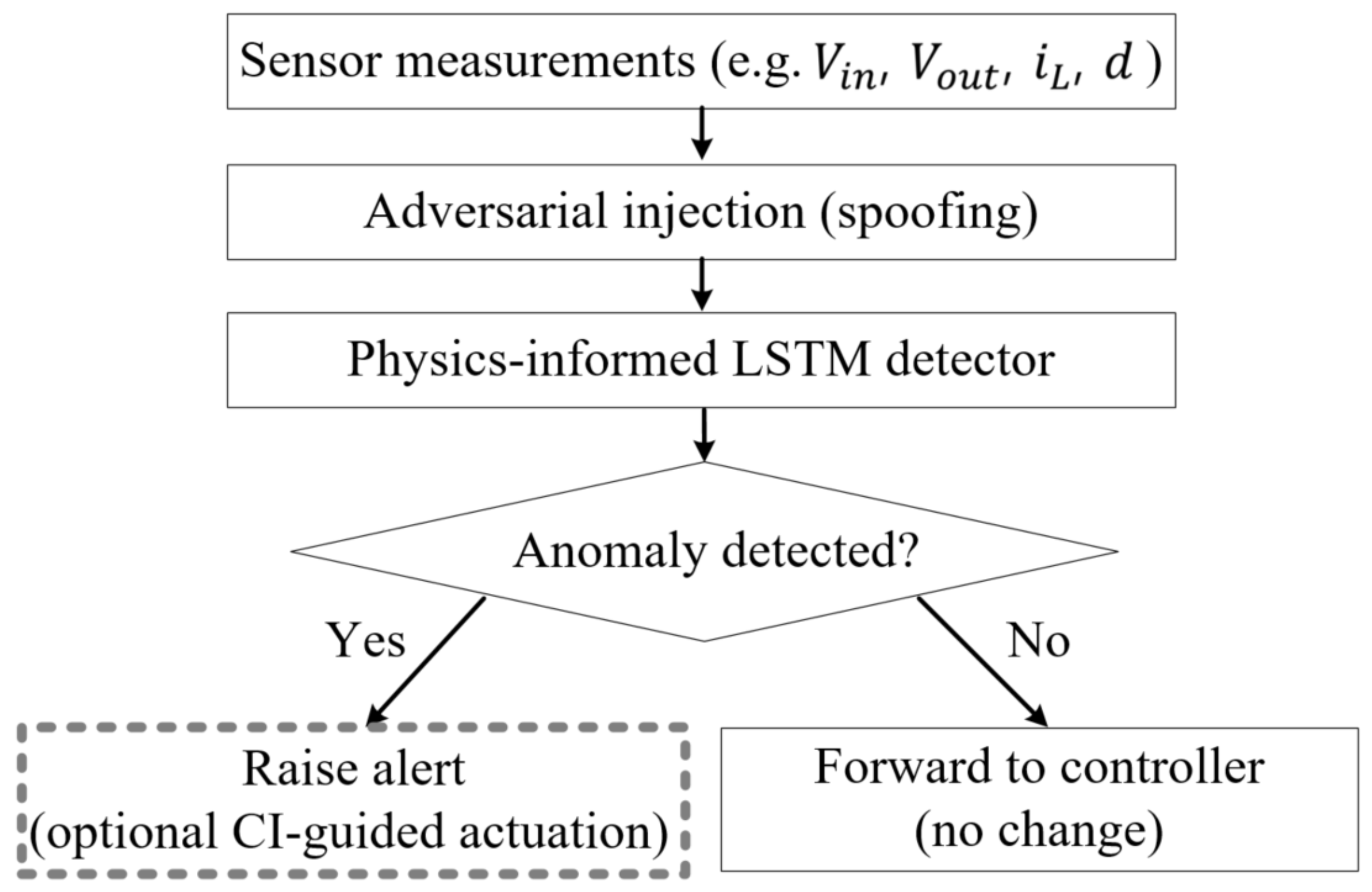
Figure 1. Flow of sensor-spoofing attacks in a cyber–physical power system (e.g., bias, delay, noise).
Applsci 15 11112 g001
Figure 2. Architecture of the proposed PI–LSTM autoencoder.
Applsci 15 11112 g002
Figure 3. Output voltage waveforms under bias, delay, and narrowband noise attacks.
Applsci 15 11112 g003
Figure 4. ROC curves of the PI–LSTM detector for the three attack types.
Applsci 15 11112 g004
Figure 5. Histograms of normalized reconstruction error s k (simulation, n = 1000 runs/attack). A dashed vertical line marks τ = μ + 3 σ computed from benign data. N = 3 consecutive- samples policy.
Applsci 15 11112 g005
Figure 6. Detection latency boxplots (simulation): n = 1000 per attack at f s = 100 kHz with L = 30 (0.30 ms). Boxes show median/IQR; whiskers 1.5 × IQR; points are outliers.
Applsci 15 11112 g006
Figure 7. CI add explanation -guided actuation (simulation): trajectory on ( V r , pp , IRR ) . The path N A D R N stays within the safety box. See Section 2.5, Equations (5) and (6).
Applsci 15 11112 g007
Figure 8. Conventional and PI–LSTM: test metrics (F1, FPR, PVR).
Applsci 15 11112 g008
Figure 9. Delay attack: anomaly score (conventional LSTM vs. PI–LSTM; simulation; N = 3 ).
Applsci 15 11112 g009
Figure 10. Experimental setup: control/power board with TI TMS320F28379D (DSP), oscilloscope measuring V out and i L , and a step-adjustable non-inductive resistive load bank.
Applsci 15 11112 g010
Figure 11. Nominal buck operation: (a) output voltage ripple; (b) inductor current.
Applsci 15 11112 g011
Figure 12. Bias injection attack: output voltage.
Applsci 15 11112 g012
Figure 13. Delay injection attack: (a) output voltage; (b) inductor current.
Applsci 15 11112 g013
Figure 14. Noise injection attack: output voltage.
Applsci 15 11112 g014
Figure 15. Anomaly score (hardware).
Applsci 15 11112 g015
Figure 16. Detection latency boxplots (hardware): n = 40 per attack at f inf = 10 kHz with L = 30 (3.0 ms). A dotted line indicates 3.0 ms (window span).
Applsci 15 11112 g016
Figure 17. Impact of attacks on DC rail quality (hardware). Bars: benign, bias, delay, noise. Reference lines denote V r , pp 240 mV , IRR 2 % , and ± 2 % regulation.
Applsci 15 11112 g017
Table 1. Prior research landscape.
CategoryRepresentative References
Model-/observer-based FDIFault diagnosis monographs and observer-based schemes [12].
Rule/statistical detectionResidual thresholds; classical change detection surveys (e.g., CUSUM/GLR) [12].
Classical ML for convertersSVM/RF/isolation forest baselines; PE monitoring surveys [13,14].
Deep time-series AEsCNN–LSTM and LSTM autoencoders in converter diagnostics [13,14].
Physics-informed learningPINNs and theory-guided data science [15,16,17,18,19,20].
CPS security in PEDevice reliability/CM and DC–DC diagnosis overviews [14,21].
Table 2. List of abbreviations used throughout the paper.
Abbrev.Definition
ADCAnalog-to-Digital Converter
AEAutoencoder
AUCArea Under the ROC Curve
CCMContinuous Conduction Mode
CIConfusion Index (policy metric; not a statistical confidence interval)
DSPDigital Signal Processor
DSODigital Storage Oscilloscope
EMI/EMCElectromagnetic Interference/Compatibility
ESREquivalent Series Resistance
FPRFalse-Positive Rate (alarm-wise unless stated)
HILHardware-in-the-Loop
IRRIn-band Ripple Ratio
LSTMLong Short-Term Memory
PI–LSTMPhysics-Informed LSTM
PSDPower Spectral Density
PWMPulse-Width Modulation
ROCReceiver Operating Characteristic
SPFSample-wise Positive Fraction
VRMVoltage Regulator Module
Table 3. Buck converter specifications.
ParameterValueUnit
Input Voltage24V
Output Voltage12V
Inductance100µH
Capacitance470µF
Load Resistance10 Ω
Switching Frequency100kHz
Output Power14.4W
Table 4. Real -world scenarios and primary effects.
DomainTypical Disturbance (Site)Primary Effect
EV (12/48 V)Supply ripple on V i n ; harness/ground; 0.5–5 kHz V r , p p , IRR  ; small regulation error unless severe; score rises at tone(s).
PV DC-linkMPPT/load transitions; sensor bias/drift (divider/ADC)Transient regulation excursions; DC shift per bias; score increases after onset.
ESS/IndustrialFixed delay τ (buffer/firmware); sense
-line EMI (≈1 kHz)
Phase margin loss ⇒ ∼ 10 2 Hz modulation (delay); narrowband component; few ms detection latency.
Notes. Arrows denote direction/effect: ↑ = increase, ↓ = decrease, and ⇒ = “leads to/manifests as.” “tone(s)” indicates narrowband spectral components at the disturbance frequency (and harmonics/sidebands) observed in the ripple metrics.
Table 5. PI–LSTM training resources and time (single-GPU run).
ItemValue
GPU/CPU/RAMRTX 5070Ti (12 GB)/Core7 255HX/64 GB
FrameworkPyTorch 2.2 (CUDA 12); data via MATLAB R2024a
Dataset windows ( L = 30 )∼180,000 (80/10/10 split)
Batch/LR schedule128/ 10 3 10 4 (cosine)
Early stoppingPatience 10 epochs
Epochs (median)35–55 (42)
Wall clock (median)65–85 min (74 min)
Peak GPU memory2.1–2.4 GB (FP32)
Checkpoint size∼7.5 MB (offline model)
Distillation time10–15 min → ( n x = 4 , n h = 32 )
Table 6. CI weights, limits, and actuation gains (unified with the safety box).
ItemValueNote
w η , w r , time , w r , freq 0.5 , 0.3 , 0.2 for [ η , V r , pp , IRR ]
240 mV , 2 % 240 mV , 2 % also used as CI normalizers
α max 0.35 deception cap
k v , k d , k f 0.04 , 0.03 , 0.05 ref/duty/freq gains
N , T hys 3 samples, 10 mspersistence/hysteresis
Table 7. Simulation parameters.
ParameterValueUnit
Simulation time0.1s
Sampling interval10µs
Total samples10,000
Attack start time50ms
Attack duration20ms
Sampling frequency100kHz
Measurement noise1%
Decision rule: see Section 4.3 for the fixed decision rule.
Table 8. Attack detection performance in simulation (mean over n = 1000 runs per attack).
MetricBiasDelayNoise
Accuracy (%)96.2491.9897.51
Precision (%)94.8390.1296.89
Recall (%)97.4593.7898.12
F1 score (%)96.1291.9197.50
Detection latency after onset (ms)2.883.952.59
Decision rule and time base: see Section 4.3 for the fixed decision rule. Hardware uses the 10 kHz inference stream with the same window L = 30 (3.0 ms).
Table 9. Classical detectors under an identical decision protocol ( τ = μ + 3 σ , N = 3 ).
MethodAccuracy (%)FPR (%)Latency (ms)Hardware (Target/Footprint)
EKF (residual)90.53.83.6–5.0MCU/DSP; state+cov <10 kB
Shewhart (residual norm)88.06.73.8–5.2MCU/DSP; negligible
Fuzzy logic (rule-based)89.05.43.5–5.0MCU/DSP; ∼10–20 rules
PI–LSTM (ours)∼95.24≤1.22.9–4.2TMS320F28379; ∼18.5 kB params
Protocol: All methods use identical windows, preprocessing, and the same decision persistence ( N = 3 ). PI–LSTM macro-average follows Table 8 (per attack: 96.24% bias, 91.98% delay, 97.51% noise).
Table 10. Windowed classifiers (SVM, RF) under an identical decision protocol.
MethodAccuracy (%)FPR (%)Latency (ms)Hardware (Target/Footprint)
SVM (linear)92.03.23.4–4.5MCU/DSP; weights <50 kB
Random Forest (200×, d 8 )93.22.53.3–4.3MCU-class feasible; ∼300 kB
PI–LSTM (ours)∼95.24≤1.22.9–4.2TMS320F28379; ∼18.5 kB
Notes. Same windows/normalization; for decision policy, see Section 4.3 for the fixed decision rule (classifier score threshold 0.5).
Table 11. Auxiliary PMSM benchmark (classical baselines; native 10 Hz; no upsampling).
MethodAccuracy (%)F1 (%)AUCFPR (%)
ARIMA 85.3 ± 1.2 83.7 ± 1.5 0.912 ± 0.005 12.8 ± 1.0
Isolation Forest 88.1 ± 0.9 86.9 ± 1.0 0.934 ± 0.004 9.5 ± 0.8
Notes. Decision rule: τ = μ + 3 σ with N = 3 consecutive samples. Confidence intervals follow the same procedure as in the main text.
Table 12. Auxiliary PMSM benchmark (neural and proposed methods; native 10 Hz; no upsampling).
MethodAccuracy (%)F1 (%)AUCFPR (%)
CNN–LSTM AE 92.5 ± 0.7 91.8 ± 0.8 0.961 ± 0.003 6.2 ± 0.6
PI–LSTM (proposed) 96 . 4 ± 0 . 5 95 . 9 ± 0 . 6 0 . 987 ± 0 . 002 3 . 5 ± 0 . 4
Notes. Same decision rule ( τ = μ + 3 σ , N = 3 ). For this auxiliary dataset, DC rail ripple metrics and ms-scale latency are not reported.
Table 13. Performance degradation under CI actuation (simulation; limits reused for normalization).
MetricNormalAfter DetectionNormalized Value
Efficiency (%)92.385.0 p η = 0.923 0.850 0.923 0.08
IRR (%)0.150.30 p r , freq = 0.30 2 % = 0.15
Output ripple V r , pp (mV)30144 p r , time = 144 240 mV = 0.60
Confusion index0 0.5 · 0.08 + 0.3 · 0.60 + 0.2 · 0.15 0.25
Normalization/limits per the unified safety box; the point stays within bounds. See Section 2.5, Equations (5) and (6).
Table 14. CI weight sensitivity at a point (same p η , p r , time , p r , freq as Table 13: 0.08 , 0.60 , 0.15 ).
Weights w η w r , time w r , freq CI (Computed)
Baseline (Table 6)0.500.300.200.25
Ripple-heavy0.300.400.300.27
Efficiency-heavy0.600.200.200.24
Equal weights0.330.330.340.26
Notes: CI varies within ± 0.03 across these settings; safety constraints remain satisfied, α max is unchanged, and attack severity ranking did not change in our runs. An extended grid and per-scenario traces are provided in Supplementary File S3.
Table 15. Conventional LSTM vs. PI–LSTM.
MetricConventional LSTMPI–LSTM
F1 score (%)89.395.2
FPR (alarm-wise, %, N = 3 )12.45.8
PVR (%)15.22.1
Table 16. IRR computation settings used in hardware measurements.
ItemSetting
Scope sampling rate≥10 MS/s
Record length≥1 Mpts
Welch estimatorHann, 50% overlap
Integration band ± 0.5  kHz around k f sw ( k = 1 5 )
Normalization V out , DC (mean of DC-coupled record)
Time-domain ripple V r , p p from AC-coupled trace (20 MHz limit)
Table 17. DSP deployment: configuration and analytic budget.
ItemValue
Model config ( n x , n h ) ( 4 , 32 )
Arithmetic/activationsFP32/PWL (DSPLib GEMM)
Per-step MACs4608
Per-step cycles (estimate)≈11 kcycles
Per-step time @ 200 MHz (estimate)≈55 µ s
Parameter memory (FP32)≈18.5 kB
Table 18. DSP deployment: measured on-board performance (TMS320F28379, 200 MHz).
ItemValue
Measured step time (median)54–58 µs ( 10 4 calls, optimized build)
Jitter (peak-to-peak)<4 µs
CPU load (LSTM only)≈55%
Streaming predictor f s = 100  kHz; decim. M = 10 ( f inf = 10  kHz); L = 30
Decision rule τ = μ + 3 σ ; N = 3 ; T hys = 10  ms
Table 19. System-level KPIs reported in addition to detection metrics.
KPISymbolUnitDefinition/Purpose
Efficiency drop η , Δ η %, %Baseline η ; Δ η = η η ; maps to CI via p η .
Ripple and spectrum V r , pp , IRR mV, %Time-domain peak-to-peak; in-band ratio around k f sw .
Regulation error | V out V | / V %Compliance to the ± 2 % DC window.
Oscillation index OI 100 150 Hz %RMS in 100–150 Hz band/ V out , DC ; delay stress proxy.
Phase margin bound PM lb deg 180 360 f c τ est (surrogate).
Alarm density AD h 1 N alarms / T obs during benign operation.
MTB alarms MTBA h T obs / N alarms .
MTT recovery MTTR sAlarm → within-limit restoration (incl. hysteresis).
Score drift SDI | μ s μ s , ref | / σ s , ref on benign segments.
Table 20. Consistency between reported and computed waveform values (nominal case).
QuantityReportedComputed (Model)Verdict
Inductor ripple Δ i L ( A p p ) 0.60 ( V i n V o u t ) D L f sw = 0.60 Consistent
Output ripple Δ v o ( V p p ) 0.03 Δ i L · ESR = 0.03 Consistent (ESR-dominant)
Bias Δ V o u t (V) 0.21 δ eff / α = 0.211 Consistent (scaled)
Delay τ (ms) 1.02 N T s = 102 × 10 µs = 1.020Consistent
Noise (1 kHz) level ( V p p )∼0.18N/AConsistent (qual.)
Table 21. Hardware detection metrics with 95% confidence intervals (representative campaign; n = 40 per attack).
AttackLatency (ms), Median [IQR]Latency, 95% CI (Bootstrap)FPR (%), 95% CI (Wilson)
Bias3.1  [2.7–3.5]2.9–3.40.8 (0.2–2.9)
Delay4.2  [3.7–4.9]3.9–4.61.2 (0.3–3.3)
Noise2.9  [2.5–3.2]2.7–3.10.6 (0.1–2.4)
Notes. Decision rule identical to deployment: threshold τ = µ + 3 σ from benign data; N = 3 consecutive samples. Intervals follow the reporting conventions already defined for simulation (Section 4.3).
Table 22. Safety box compliance summary (limits: | V o u t V | ± 2 % , V r , p p 240 mV, IRR 2 % ).
ScenarioDC Regulation
( | V out V | ± 2 % )
V r , pp 240 mV IRR 2 %
Hardware (no CI actuation)Fail (delay, up to 2.8 % )PassPass
Simulation (with CI actuation)PassPassPass
Notes. In the body cells, Fail indicates a safety-box violation of the stated limits; “Pass” denotes compliance. In the hardware run without CI actuation, only the DC regulation briefly exceeded the ± 2 % window under the delay attack (peak 2.8 % ), while V r , p p and IRR remained within limits.
Disclaimer/Publisher’s Note: The statements, opinions and data contained in all publications are solely those of the individual author(s) and contributor(s) and not of MDPI and/or the editor(s). MDPI and/or the editor(s) disclaim responsibility for any injury to people or property resulting from any ideas, methods, instructions or products referred to in the content.