Article

Enhanced UAV Trajectory Tracking Using AIMM-IAKF with Adaptive Model Transition Probability

1
School of Mechanical and Electrical Engineering, North University of China, Taiyuan 030051, China
2
Institute of Intelligent Weapons, North University of China, Taiyuan 030051, China
3
Chengdu Lingchuan Special Industries Co., Ltd., Chengdu 610105, China
4
School of Mechanical Engineering, North University of China, Taiyuan 030051, China
*
Author to whom correspondence should be addressed.
Appl. Sci. 2025, 15(20), 11111; https://doi.org/10.3390/app152011111
Submission received: 1 September 2025 / Revised: 5 October 2025 / Accepted: 14 October 2025 / Published: 16 October 2025

Abstract

In complex Unmanned Aerial Vehicle (UAV) trajectory tracking scenarios, conventional Interacting Multiple Model (IMM) algorithms face challenges such as slow model switching rates and insufficient tracking accuracy. To address these limitations, this paper proposes an enhanced algorithm named Adaptive Interacting Multiple Model-Improved Adaptive Kalman Filter (AIMM-IAKF). The AIMM component dynamically adjusts the model transition probability matrix based on real-time model probability differences, overcoming the limitation of a fixed matrix in traditional IMM. Furthermore, the conventional Kalman filter is replaced with an Improved Adaptive Kalman Filter (IAKF), which introduces a convergence criterion and a suboptimal fading factor to optimize noise statistics. Simulation results demonstrate that, compared to the traditional IMM algorithm, the proposed AIMM-IAKF algorithm improves tracking accuracy by approximately 69%, achieves a faster model switching response, and exhibits superior stability with lower error fluctuation. The proposed framework provides a highly accurate and robust solution for tracking highly maneuvering UAVs.

1. Introduction

As unmanned aerial vehicles (UAVs) increasingly integrate into the Internet of Things (IoT) ecosystem [1], their capabilities have evolved from basic aerial platforms to intelligent entities capable of real-time monitoring, delivery, and urban mobility [2,3]. This evolution imposes stringent demands on reliable trajectory tracking under complex airspace constraints [4]—particularly in high-density low-altitude environments where safety, adaptability, and robustness are paramount [5]. However, traditional trajectory tracking methods often lack adaptability under uncertain conditions; despite extensive research into related technologies, achieving high-precision tracking remains a persistent challenge when confronted with noise, data sparsity, and maneuver dynamics [6,7,8]. These challenges are especially prominent in military scenarios [9], where UAVs demonstrate exceptional practical value due to their high flexibility, autonomy, and cost-effectiveness [10]. During the Ukraine conflict, UAVs were deployed not only for direct combat operations but also excelled in reconnaissance and surveillance missions [11] and are projected to become indispensable assets in future conflicts [12]. To address these challenges, Artificial Intelligence-based enhanced models have emerged [13], employing specialized activation functions and hybrid mechanisms to handle nonlinear dynamic issues [14]. Yet such approaches suffer from significant limitations: constrained generalization, poor online adaptability, and struggles with insufficient real-world UAV data, substantial noise, and the need to track targets beyond training data boundaries—rendering them unreliable for critical missions under non-stationary and uncertain conditions [15]. Current trajectory tracking methods fall into two main categories: traditional Kalman filter-based approaches [16], which are widely adopted in power systems [17,18], navigation and positioning [19,20], and target tracking [21,22] due to their fast convergence, high reliability, and ease of implementation; and machine learning-based approaches [23,24]. Given the limitations of machine learning methods, they struggle to meet the demands of critical scenarios. Thus, this paper focuses on trajectory tracking research based on traditional methods.
Traditional Kalman filtering requires accurate pre-setting of noise characteristics [25]. However, in real-world scenarios like UAV trajectory tracking, trajectories are often non-stationary due to environmental perturbations. To address this issue, Filho et al. [26] utilizes online estimation of noise covariance to dynamically adapt to noise process, thus obviating the need for reliance on predefined noise characteristics. Akbaş et al. [27] integrates Kalman filtering with an adaptive filter incorporating a fading factor to mitigate errors and bias rates. Cheng et al. [28] adopts an adaptive factor to rectify system noise covariance in real time, thereby enhancing navigation accuracy in complex environments. Sun et al. [29] advocates adaptive updates to the noise covariance matrix under data anomalies, alleviating filter divergence and improving positioning accuracy. These studies demonstrate that adaptive Kalman filters can overcome traditional limitations and reduce noise impact through adaptive updates. However, their performance is constrained by single-model limitations. In contrast, the Interacting Multiple Model (IMM) algorithm achieves more accurate state estimation by interactively fusing multiple models, offering superior robustness and flexibility.
The IMM algorithm, based on a finite-state Markov chain, employs a probabilistic transfer mechanism to process multiple model states interactively, enabling rapid model switching [30]. Granstrom et al. [31] proposed a novel mode-mixing method aligned with current matching models, adapting to target maneuvering in 3D space without altering the system model. Baofeng Zhao [32] studied maneuvering target motion model uncertainties and sensor error correlations, proposing an IMM-based information fusion algorithm and an IMM information decorrelation algorithm, both validated for effectiveness. Wang et al. [33] introduced the generalized interacting multiple model Kalman filter (GIMM-KF) algorithm, addressing target tracking in non-Gaussian noise environments by incorporating a Gaussian mixture model to improve accuracy. Yang et al. [34] proposed the Interactive Multiple Model Adaptive Robust Kalman Filter (IMMARKF) algorithm, combining robustness, adaptivity, and optimality to handle complex maneuvering trajectories under model and measurement errors. However, when estimating the state of complex maneuvering target, the traditional interacting multiple model Kalman filter (IMM-KF) algorithm encounters two major issues: (1) The transfer probability matrix parameters are fixed and preset, failing to account for dynamic probability adjustments, which hinders rapid switching to the target’s true motion model, causing tracking errors and delays; (2) With short measurement sampling intervals, noise and interference effects cannot be accurately modeled, rendering the traditional Kalman filter inadequate for precision requirements. Xie et al. [35] improved response speed and estimation accuracy by introducing a correction function for adaptively transferring probability adjustments but did not optimize filter performance further. Sun et al. [36] proposed an IMM algorithm combining adaptive factors, demonstrating enhanced adaptability and stability in noisy environments, though computational resource wastage occurs with stable noise statistics. (Lee and Park [37] improved tracking accuracy by adaptively updating the Markov transfer probability matrix via polarization and activation jump probability correction functions but did not optimize noise characteristics, leaving room for improvement.
These limitations underscore the need for a trajectory tracking framework capable of simultaneously addressing noise uncertainty and model-switching inefficiency. In response, this paper proposes an enhanced algorithm—Adaptive Interacting Multiple Model Improved Adaptive Kalman Filter (AIMM–IAKF)—which combines the adaptive measurement update mechanism of IAKF with the model fusion capability of IMM. To overcome the rigidity of conventional fixed Markov transition matrices, an adaptive transfer probability correction function is introduced, enabling dynamic adjustment based on real-time model probability variations. Furthermore, an improved IAKF structure incorporating a convergence criterion and a suboptimal fading factor is employed to optimize noise statistics within each model component. The proposed tracking algorithm can be applied to UAVs performing missions in urban environments involving reconnaissance, package delivery, and collision avoidance. The maneuvers in these tasks require seamless integration of Constant Velocity (CV), Constant Acceleration (CA), and Constant Turn (CT) rate models. Comparison of related work and proposed method is shown in Table 1.
The proposed AIMM–IAKF framework enhances tracking accuracy, responsiveness, and robustness in complex UAV maneuvering scenarios. Its effectiveness is validated through extensive simulations involving highly dynamic target trajectories. The remainder of this paper is organized as follows: Section 2 outlines the target motion model. Section 3 details the UAV trajectory tracking algorithm, analyzing the Kalman filter, its limitations, and the IMM algorithm, with a focus on transfer probability matrix impacts and filter selection. Section 4 presents UAV trajectory tracking simulations, analyzing results to verify the feasibility and efficiency of the proposed approach. Section 5 summarizes the research and discusses future directions.

2. The Improved Adaptive Kalman Filter: From Foundations to Implementation

2.1. UAV Motion Models

The tracking target in this study is the UAV, whose motion, being stochastic due to the influence of algorithms and external factors, renders precise modeling infeasible. Thus, established models are employed to approximate its real-time motion [38]. To align with UAV swarm behaviors such as uniform linear motion, uniformly accelerated linear motion, uniform turns, and dive attacks, the Constant Velocity (CV), Constant Acceleration (CA), and Constant Turn (CT) models are adopted as tracking models.
The CV model functions as a simplified kinematic model for the uniform linear motion of UAVs. By assuming velocity remains approximately constant over short time intervals, it offers a tractable approximation for linear motion affected by external disturbances or modeling uncertainties, which induce random velocity perturbations. Its state-space equation is expressed as:
X k + 1 = Φ V X k , Φ V = 1 T 0 0 1 0 0 0 1
where X k + 1 is the state vector at time k + 1, and Φ V denotes the state transition matrix for the UAV’s uniform motion. T is the sampling interval. Yet this model is confined to low-maneuver scenarios; for motions with acceleration, it needs to be extended to the CA model. To characterize linear motion with approximately constant acceleration, acceleration is incorporated into the state vector, resulting in the CA model. The state-space equation of the CA model is expressed as:
X k + 1 = Φ A X k , Φ A = 1 T T 2 / 2 0 1 T 0 0 1
where Φ A denotes the state transition matrix for the drone’s uniformly accelerated motion. Yet the CA model remains a linear model that cannot characterize nonlinear maneuvers such as turning, thus requiring the introduction of the CT model. The CT model assumes a constant angular velocity ω during short-term turns, enabling it to account for the nonlinear coupling between x-axis and y-axis motions [39].
As shown in Figure 1, the target is assumed to undergo three-dimensional motion, performing a circular trajectory in the X Y directions while maintaining its original motion state along the Z direction. At time t , the target’s velocity v t can be decomposed into components v x t and v y t along the x and y directions, respectively. The motion is characterized by a tangential acceleration a t and a centripetal acceleration a u , with the direction of motion defined by the heading angle ψ , whose rate of change is the turn rate ω (i.e., ω = d ψ / d t ). The target is moving in the X and Y directions as follows. The kinematic behavior of the target in the X Y axis is described as follows:
a x = v y ω a y = v x ω
To implement in a recursive filter, the state-space equation of the CT model is expressed as:
X k + 1 = Φ C T X k , Φ C T = 1 s i n ( ω T ) / ω 0 0 ( c o s ( ω T ) 1 ) / ω 0 0 0 0 0 c o s ( ω T ) 0 0 s i n ( ω T ) 0 0 0 0 0 0 1 0 0 0 0 0 0 0 ( 1 c o s ( ω T ) ) / ω 0 1 s i n ( ω T ) / ω 0 0 0 0 0 s i n ( ω T ) 0 0 c o s ( ω T ) 0 0 0 0 0 0 0 0 0 1 0 0 0 0 0 0 0 0 0 1 T 0 0 0 0 0 0 0 0 1 0 0 0 0 0 0 0 0 0 1
where Φ C T 9 × 9 is the exact state transition matrix. The CT model captures planar maneuvering characteristics via the yaw rate ω, while modeling z-axis vertical motion as an independent sub-dynamic. Each of the CT, CV, and CA models is paired with a Kalman filter; in subsequent interactive multi-model filtering, these model–filter combinations collaboratively estimate the target state across varying maneuver conditions.

2.2. Basic Filtering Algorithms and Improvements

Motion models mathematically capture the typical maneuvering characteristics of UAVs. However, due to simplifying assumptions and random disturbances, they necessitate integration with filtering algorithms to achieve precise trajectory estimation. As an optimal recursive estimation algorithm, the Kalman filter’s “predict-update” mechanism fuses model prior information with measurement data: motion models (e.g., CV, CA, CT) provide state transition matrices to underpin state prediction in filtering; the filter then suppresses noise via measurement correction, enabling optimal state estimation.

2.2.1. Standard Kalman Filter

The Kalman filter is an optimal recursive estimation algorithm for linear dynamic systems. It operates through a cyclic two-step process: prediction of the system state followed by measurement update. The fundamental principle of Kalman filtering lies in its ability to optimally combine priori state estimates (predictions based on previous states) with posteriori information (corrected estimates incorporating new observations) through minimum mean-square error estimation.
The UAV trajectory tracking system can be expressed by the following system equations:
X k + 1 = Φ k X k + Γ k ω k Z k + 1 = H X k + 1 + υ k
where X k + 1 is the system state quantity at time k + 1 , Φ k is the state transfer matrix at time k , Γ k is the system noise coefficient matrix, ω k is the system noise vector at time k + 1 , υ k is the measurement noise vector at time k + 1 , H is the observation matrix, and Z k + 1 is the measurement state quantity at time k + 1 . The operational framework of the discrete-time Kalman filtering algorithm is illustrated in Figure 2.
As shown in Figure 2, the diagram comprises two circuits: the Filter Calculation Circuit and the Gain Calculation Circuit. The Filter Calculation Circuit undertakes the iterative update of state estimation, whereas the Gain Calculation Circuit is dedicated to computing the Kalman gain. Where Q is the system noise covariance matrix and R is the measurement noise covariance matrix, the specific algorithm steps of the discrete Kalman filtering algorithm are as follows:
A priori state estimation
X ( k + 1 / k ) = Φ k X ( k / k )
where X ( k + 1 / k ) is the a priori estimate of the state at time k + 1 , Φ k is the state transfer matrix at time k , and X ( k / k ) is the state prediction at time k .
A priori covariance estimation
P ( k + 1 / k ) = Φ k P ( k / k ) Φ k T + Γ k Q Γ k T
where P ( k + 1 / k ) is the updated a priori state covariance at time k + 1 , P ( k / k ) is the state covariance at time k , and Q is the system noise covariance matrix.
Calculate the filter gain matrix
K k + 1 = P ( k + 1 / k ) H T H P ( k + 1 / k ) H T + R 1
where K k + 1 is the gain matrix obtained at time k + 1 based on the minimum variance principle, H is the observation matrix, and R is the measurement noise covariance matrix.
Calculate the state estimate at time k + 1
X ( k + 1 / k + 1 ) = X ( k + 1 / k ) + K k + 1 Z k + 1 H X ( k + 1 / k )
where X ( k + 1 / k + 1 ) is the updated state value prediction at time k + 1 and Z k + 1 is the measured state quantity at time k + 1 . The state value prediction at time k + 1 is the updated state value prediction at time k + 1 .
Calculate the variance of the estimation error at time k + 1 .
P ( k + 1 / k + 1 ) = I K k + 1 H P ( k + 1 / k )
where P ( k + 1 / k + 1 ) is the updated state covariance at time k + 1 . The system state and state covariance are updated by Equations (9) and (10) for the next cycle.
The Kalman filter demonstrates superior response speed, enabling real-time state estimation while effectively attenuating noise measurement. This optimal estimator provides a more accurate system state estimation through its recursive prediction-correction mechanism.

2.2.2. Improved Adaptive Kalman Filter

The standard Kalman filter (KF), a linear optimal recursive estimation algorithm, enables state estimation via its “predict-update” mechanism. However, its performance is strongly reliant on prespecified noise covariance matrices Q and R . In UAV trajectory tracking scenarios, KF has two key limitations: First, measurement noise in real-world environments (e.g., airflow disturbances, sensor errors) is non-stationary, rendering a fixed R poorly adapted to abrupt noise variations. Second, it lacks a criterion for determining filter convergence, continuing to update covariances even once steady state is reached—this may introduce numerical perturbations and computational redundancy.
To mitigate these limitations of KF, this paper presents an Improved Adaptive Kalman Filter (IAKF) algorithm, with the following core innovations:
Introduce a residual-based convergence judgment threshold.
ε k ε K T H P ( k + 1 / k ) H T + R
ε k = Z k + 1 H X ( k + 1 / k )
S k = H P ( k + 1 / k ) H T + R
where ε k represents the deviation between the observed value and the state estimate, while S k denotes the innovation covariance—specifically, the sum of the observation projection transformation of the prior covariance matrix and the observation noise covariance matrix. When this condition is met, it indicates an imbalance in the filter’s confidence, specifically an over-reliance on the observations. This imbalance violates the optimality assumptions of the Kalman filter. If left uncorrected, the estimation error will accumulate over successive iterations, ultimately leading to filter divergence. At this point, the system noise covariance Q and measurement noise covariance R should be updated. If the condition is not satisfied, the current model is deemed to match the UAV’s motion state, thereby reducing unnecessary computational overhead and avoiding numerical perturbations.
Suboptimal fading factor adjustment: Employing a suboptimal fading factor in the interval λ k , combined with the weighting coefficient b k = 1 λ k / 1 λ k k + 1 , enables dynamic updating of noise covariance:
The measurement noise covariance R is updated as:
R k = ( 1 b k ) R k + 1 + b k ( ε k ε k T H P k + 1 / k H T )
The system noise covariance Q is updated as:
Q k = ( 1 b k λ k ) Q k 1 + b k λ k k ( K k + 1 ε k ε k T K k + 1 T + P k + 1 Φ k P k + 1 / k Φ k T )
where the suboptimal fading factor enhances sensitivity to new observations through an “exponential forgetting” weighting mechanism applied to historical data, thereby reducing the weight of outdated information. The introduction of b k redirects the optimization process to prioritize recent data. λ k is constrained within the interval [0.95, 0.995]. The value of the suboptimal fading factor λ k is empirically determined through simulations, a design choice that optimally balances the need for swift covariance updates against the imperative of algorithmic stability. The lower bound of 0.95 ensures a rapid response to abrupt noise, balancing responsiveness with the avoidance of excessive sensitivity; the upper bound of 0.995, on the other hand, guarantees filter stability and smoothness, enabling both steady-state smooth output and adaptability to slowly varying noise. The observation noise covariance R k is updated by integrating the historical information retention term, the second-order moment of innovations, and the observation projection of prediction errors: When the actual measurement noise increases and the actual error energy exceeds the model’s expectation, R k increases under the weighting of R k to reduce the confidence in observations. Conversely, when the noise decreases, R k decreases to enhance confidence, thereby achieving adaptive tracking of time-varying observation noise through “historical smoothing” and “innovation correction”. The system noise covariance Q k is updated via a formula that incorporates historical information retention terms, decay weights of new information, contributions of observational correction errors, and deviations of model prediction errors: When the deviation between the model and actual motion increases, positive correction terms lead to an increase in Q k to enhance the compensation for model errors; when the model matches the actual motion well, Q k remains stable. This realizes adaptive tracking of system dynamics through “historical stabilization” and “recent deviation correction”.
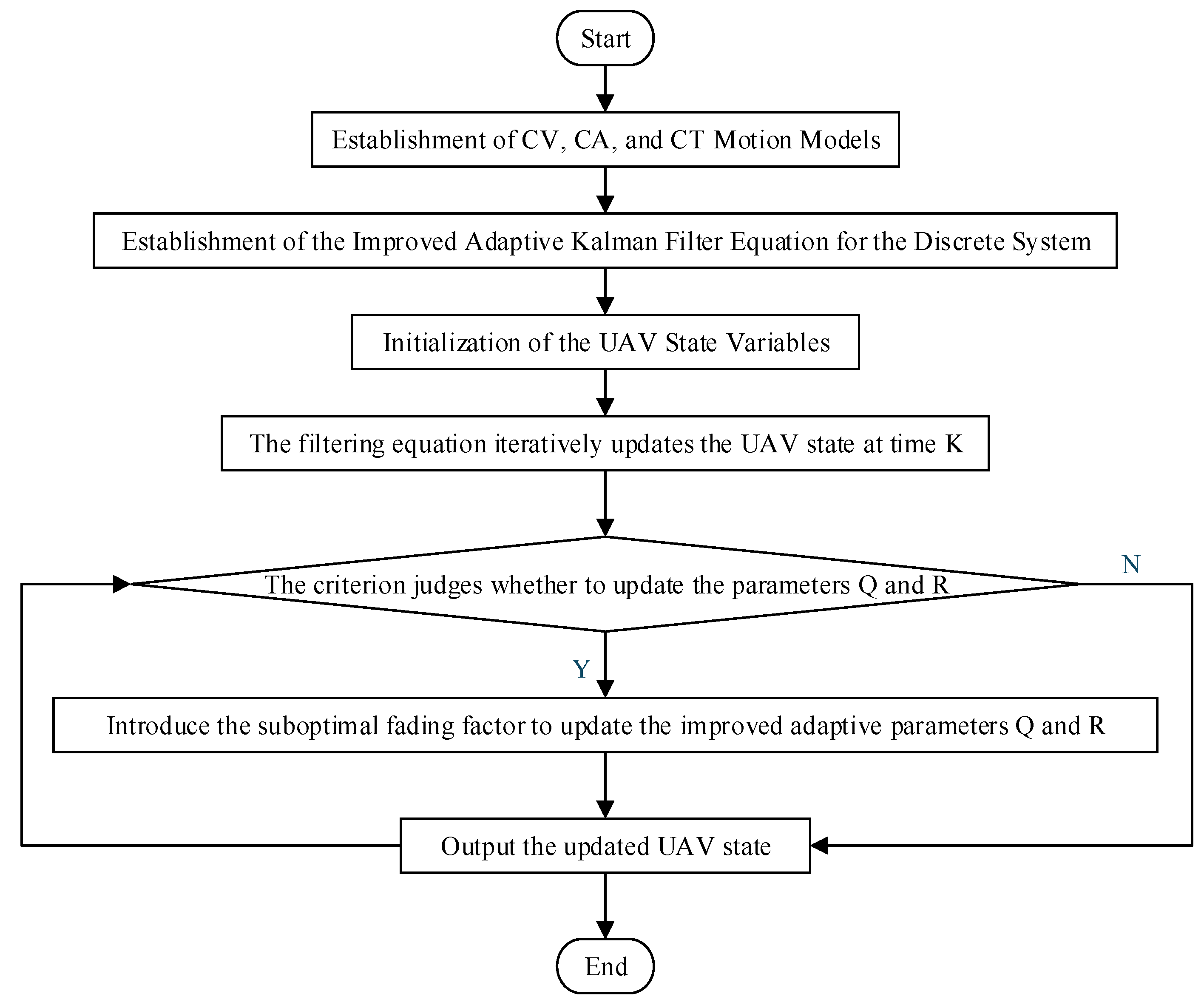
These updates ensure that the covariances Q k and R k can adapt in real time to changes in system dynamics while suppressing the influence of outdated information. The fading scheme enables convergence toward a stable noise estimate, improving estimation robustness under non-stationary noise conditions. The overall estimation process is illustrated in the IAKF flowchart shown in Figure 3.
The proposed UAV trajectory tracking framework based on the IAKF consists of six main stages, as illustrated in Figure 3. First, a set of baseline motion models including CV, CA, and CT are established to characterize the UAV’s maneuvering behavior. Then, the discrete-time formulation of the IAKF is constructed to support online state estimation with adaptive noise updates. The system initialization step defines the initial values of the UAV state vector. Subsequently, the Kalman filter equations are iteratively applied to propagate and correct the state estimates at each discrete time step k . A convergence criterion is evaluated at every iteration to determine whether the adaptive noise parameters Q k and R k require updating. If the criterion is met, a suboptimal fading memory factor λ k is used to weigh recent innovations more heavily and gradually suppress the influence of older data. The updated covariances are then used in subsequent filtering steps. Finally, the updated UAV state at time k + 1 is output for downstream processing, such as motion control or trajectory refinement.

3. The Adaptive IMM (AIMM) Strategy: Formulation and Integration

3.1. Basic IMM Algorithm

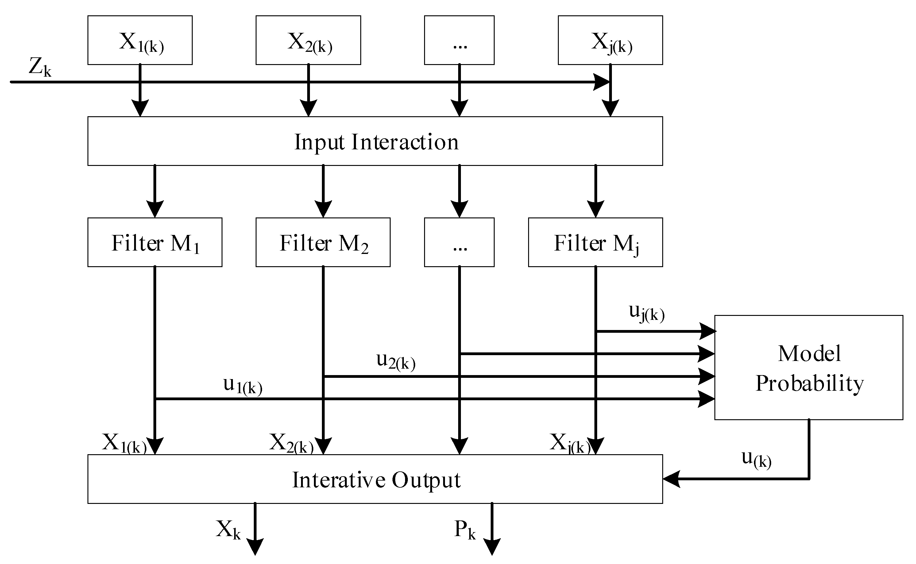
The basic IMM [40] is an adaptive filtering approach that incorporates multiple motion models for target tracking. This algorithm operates by simultaneously executing parallel state predictions using different motion models. Subsequently, it computes a weighted fusion of all model outputs based on their respective matching probabilities with the observed target behavior, thereby achieving robust target tracking. In this paper, we use the CV motion model, the CA motion model, and the CT model as the base models for this algorithm to interact with, while the filtering results will be used as inputs for the next moment in time. Figure 4 illustrates this working principle schematically.
In the IMM algorithm, the switching process among multiple motion models essentially follows a first-order discrete-time Markov chain. This assumption forms the theoretical foundation for the stable operation of the IMM algorithm. That is:
P ( M k = M j M k 1 , M k 2 , , M 0 ) = P ( M k = M j M k 1 )
indicates that the current model M k Mk at the current time is only related to the previous model M k 1 and is unrelated to earlier history. The experimental setup in this paper includes three candidate motion models, with the Markov model transition matrix defined as:
Π = p i j , p i j = P ( M k = j M k 1 = i )
where represents the transition probability from model to model, and the sum of the probabilities in any row satisfies the normalization condition:
j = 1 N p i j = 1 , i 1 , 2 , 3
This matrix defines the switching probabilities between models and is a key parameter in the IMM filtering process.
The IMM algorithm operates by computing a weighted fusion of state estimates from multiple parallel model-based filters to produce an optimal combined estimate. Each iteration cycle of the algorithm executes four key computational stages: (1) model-conditional initialization and reinitialization; (2) model-conditional filtering; (3) model probability updating; (4) interactive output synthesis. For any model m i M k 1 , the algorithm’s cyclic estimation process is mathematically characterized by the following expression:
(1) Model condition initialization and reinitialization
Predictive modeling probabilities:
μ j ( k 1 ) = m i M k 1 Π i j μ j ( k 1 )
Weight normalization:
Π i j = Π i j μ i ( k 1 ) / μ j ( k 1 )
Mixed Estimates:
X j 0 = m i M k 1 X i ( k 1 ) Π i j
Mixed Covariance:
P j 0 = m i M k 1 P i ( k 1 ) + ( X i ( k 1 ) X j 0 ) ( X i ( k 1 ) X j 0 ) T Π i j
where Π i j is the model transfer probability from model i to model j , X i ( k 1 ) is the output of filter i at time k 1 and P i ( k 1 ) is its corresponding covariance matrix, X j 0 is the mixture estimate of model j at the current moment and P j 0 is its corresponding mixture covariance matrix.
(2) Model Conditional Filtering
The filtering results obtained from the above two equations are used as input variables to match the model m j at the next moment, and then the three filter performs state filtering according to its own algorithm to obtain its own state estimate X j ( k ) and covariance P j ( k ) .
(3) Model probability update
Likelihood function:
L j ( k ) = N Z ˜ j ( k ) ; 0 , S j ( k )
Updating the probability model:
μ j ( k ) = μ j ( k 1 ) L j ( k ) m j M k 1 μ j ( k 1 ) L j ( k )
where Z ˜ j ( k ) and S j ( k ) are the new interest rate and its covariance of model j at time k , respectively, and N x ; x ¯ , σ 2 denotes that the random variable x obeys a normal distribution with mean x ¯ and variance σ 2 .
(4) Interactive output
Overall estimate:
X k = m j M k X j ( k ) μ j
Overall covariance:
P k = m j M k P j ( k ) + ( X j ( k ) X k ) ( X j ( k ) X k ) T μ j
The IMM algorithm operates under the assumption that one model optimally represents the current system conditions. The process begins by computing initial conditions for each model-matched filter through state estimation mixing from all previous filter states. This is followed by parallel filtering across all models to generate individual state estimates. Subsequently, the algorithm updates model probabilities using likelihood function evaluations and combines the adjusted state estimates to produce the final output. Two critical factors determine the ultimate tracking accuracy: (1) the effectiveness of filter updates; (2) the precision of model probability calculations. However, conventional IMM implementations exhibit a significant limitation: they typically employ a static transition matrix predetermined by prior knowledge or manual selection. This fixed approach fails to account for the dynamic nature of model transitions, consequently compromising both: (1) the adaptability of model probability updates; (2) the overall tracking performance.

3.2. AIMM Algorithm

To tackle the limitation that traditional IMM algorithms neglect the dynamic rationality of transition probability matrices, this paper proposes a novel transition probability adjustment function, which allows the target to better match the current motion state in real time. This method estimates unknown transition probabilities using the difference in model probabilities of the sub-motion model between consecutive time steps ( k 1 and k ). For the j th tracking sub-motion model, if its model probabilities at time steps k and k 1 are μ j k and μ j k 1 , respectively, the model probability difference Δ μ j k directly reflects the variation in the degree of matching between sub-motion model j and the true trajectory at successive time points. Furthermore, the function integrates a transition probability speed adjustment factor to control the adaptation rate of the probability. The transition probability adjustment function is expressed as follows:
F i j k = e Δ μ j ( k ) log 10 α
Δ μ j k = μ j k μ j ( k 1 )
where F denotes the transition probability adjustment function, and F i j ( k ) represents the element in the i th row and j th column at time step k . α is the speed parameter of the adjustment function. Notably, when 0 < α < 1 , this changes the sign of Δ μ j k , thereby reversing the feedback direction of the adaptive adjustment. As a result, the probability of selecting the correct motion model may decrease, while the probability of selecting an inappropriate model may increase. When α = 1 , the method reduces to the original IMM algorithm. When 1 < α < 10 , the adjustment speed becomes slower; in contrast, when α > 10 , the adjustment speed increases. While the parameter α is typically set to 10 by default, its value requires careful adjustment in practice to compensate for errors introduced by varying model transition rates. The enhanced function offers an expanded adjustment range and more precise rate tuning capabilities, significantly improving debugging efficiency and optimization flexibility.
For an IMM algorithm containing M motion models in its model set, the construction process of the model correction function adjustment method proceeds as follows:
Calculate the same model probability change:
Δ μ j k = μ j k μ j ( k 1 ) , j = 1 , 2 , M
where μ j k represents the model probability of motion model j at time k.
Update to improve tuning functions:
F i j k = e Δ μ j k log 10 α , i , j = 1 , 2 M
Fix the state transition probability:
p i j k = F i j k p i j ( k 1 ) , i = 1 , 2 M
where p i j ( k 1 ) denotes the transfer probability from motion model i to motion model j at time k 1 Normalization:
p i j k = p i j k j = 1 M p i j k , i , j = 1 , 2 M
Moreover, after normalization, the improved transition probability matrix still achieves the Markov chain:
j = 1 M p i j k = 1 , i , j = 1 , 2 M
From Equations (29)–(31), it can be seen that when Δ μ j k > 0 , it means that the motion model j is closer to the target’s real motion model at this time, the motion model at this time is in the holding stage, and F i j k > 1 , the model probability increases, the improved adjustment function realizes the purpose of increasing the proportion of matched models, and then achieves the purpose of improving tracking accuracy. When Δ μ j k < 0 , it means that the motion model j is not matched with the real motion model of the target at this time, and the motion model is in the switching stage, and F i j k < 1 , the probability of the model decreases, the improved adjustment function realizes the purpose of increasing the proportion of matching model, accelerating the stabilization of the model switching rate, and then achieving the purpose of improving the tracking accuracy.
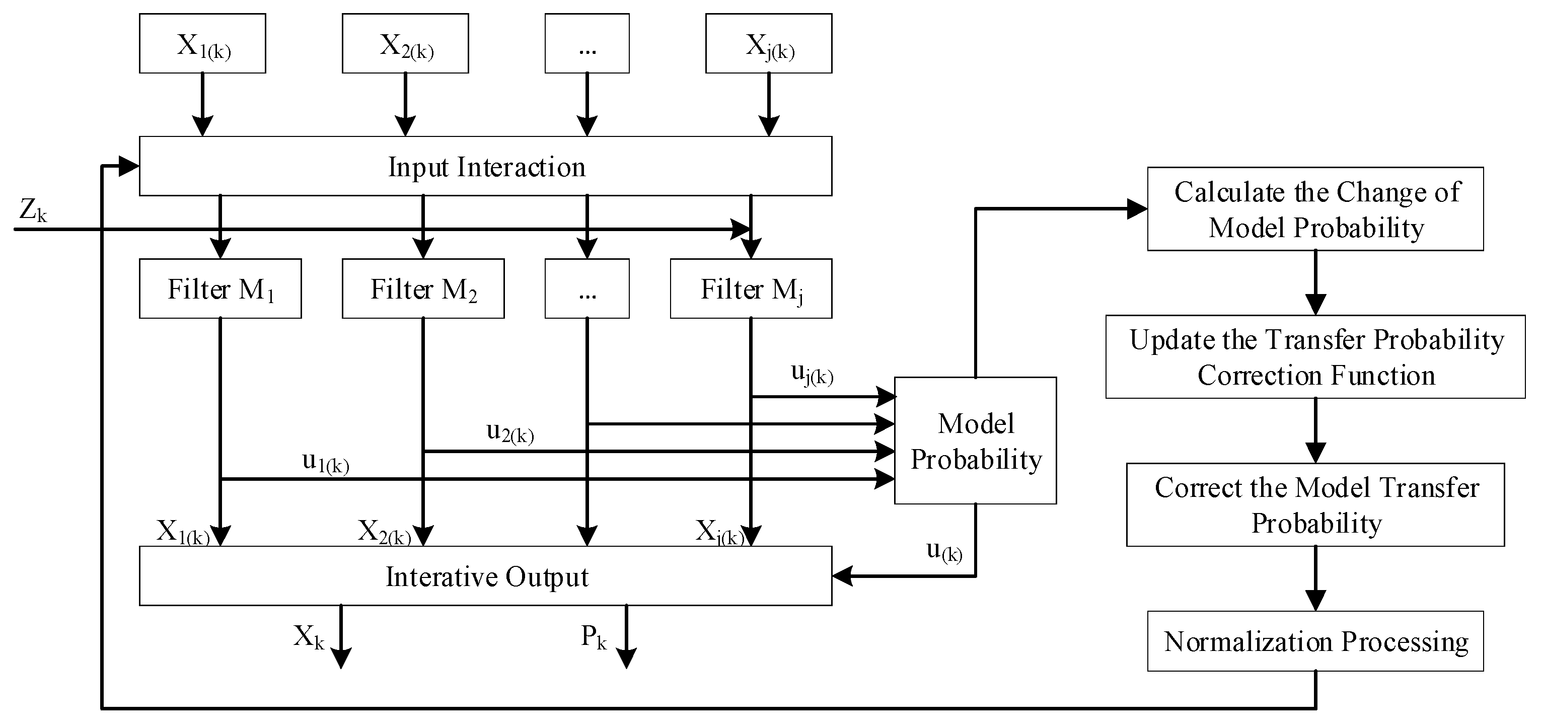
The transfer probability matrix is adaptively adjusted by applying appropriate coefficients through the above steps, while integrating historical model information to update the transition probabilities. Figure 5 illustrates the working principle of this adaptive switching mechanism for the IMM algorithm.
Figure 5 demonstrates how the enhanced correction function enables dynamic updating of the Markov matrix based on model matching performance. This modification rapidly boosts the matching model’s probability during transition periods, effectively minimizing errors caused by model switching mismatches. Furthermore, the improved function enhances the IMM algorithm’s noise resistance when operating under a consistent system model.

3.3. UAV Trajectory Tracking Using AIMM-IAKF Algorithm

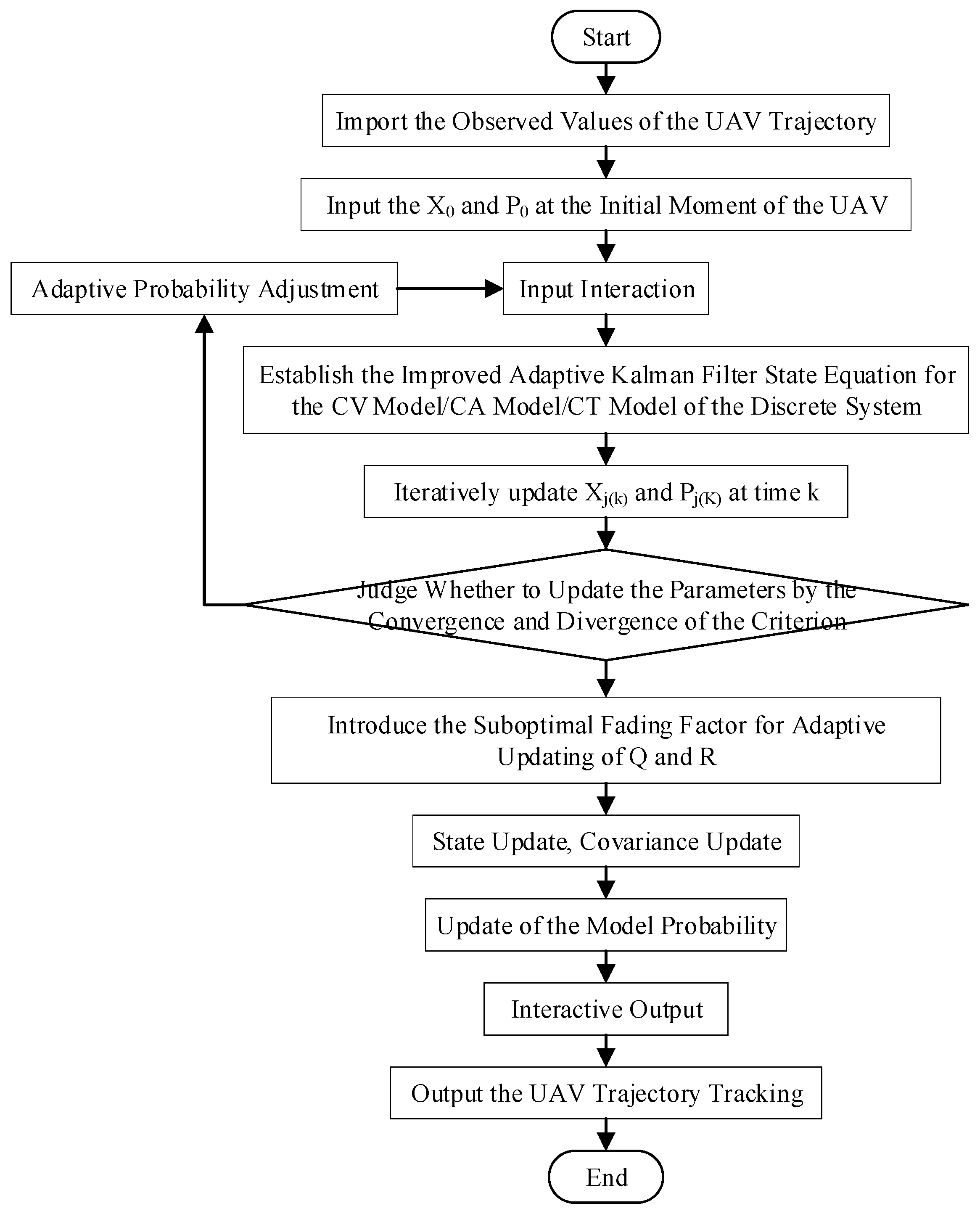
By integrating the enhanced capabilities of both the IAKF and the AIMM algorithm, a comprehensive UAV trajectory tracking framework based on the Adaptive Interacting Multiple Model-Improved Adaptive Kalman Filter (AIMM-IAKF) approach is developed, as illustrated in Figure 6.
The processing pipeline begins by initializing the UAV trajectory model, which first undergoes input interaction fusion. The fused results are then processed through our IAKF, incorporating CV, CA, and CT motion models, to generate preliminary state estimates. Subsequently, the AIMM module updates model probabilities based on these estimates while adaptively adjusting the transition matrix for optimal tracking. The cycle concludes with interactive output fusion, producing refined UAV trajectory tracking values and preparing the system for the next filtering iteration. The pseudocode for the AIMM-IAKF algorithm is shown in Algorithm 1:
Algorithm 1: The AIMM-IAKF Algorithm
Input: Initial state X0, covariance P0, model set M = {CV, CA, CT}, initial model probabilities μ0, initial transition matrix Π0.
Output: Fused state estimate Xk, covariance Pk.
1: for each time step k do
2:     // AIMM: Input Interaction (Mixing)
3:    Calculate mixed estimates Xj(0) and covariances Pj(0) for each model using Equations (19)–(22).
4:     // Parallel IAKF Filtering
5:    for each model j in M do
6       Perform prediction step using Xj(0) and Pj(0).
7:        // IAKF Adaptation
8:       Compute innovation εk and innovation covariance Sk.
9:       if convergence criterion (Equation (11)) is violated then
10:     Calculate weight bk based on the fading factor λk.
11:     Adapt Qk and Rk using Equations (14)–(15).
12:     end if
13:   Perform update step to get Xj(k) and Pj(k).
14:   Compute model likelihood Lj(k) (Equation (23).
15:   end for
16:    // AIMM: Probability Update & Adaptive Transition Matrix
17:   Update model probabilities μj(k) (Equation (24).
18:   Adapt the transition matrix Π using the new probabilities and Equations (27)–(33).
19:    // Output Fusion
20:   Fuse state and covariance estimates across all models (Equations (25)–(26) to get Xk and Pk.
21: end for

4. Results and Discussion

4.1. Simulation Setup

This study simulates UAV trajectories based on the kinematic characteristics of intercepting and dive-bombing UAVs from Reference [41], which represent highly maneuverable targets combining CV, CA, and CT motion models. In this paper, the initial state covariance of the tracking algorithm is set as P 0 = 100 I 1 , where I 1 is the identity matrix of dimension 9 × 9 ; the initial system noise covariance Q is Q = eye ( 3 ) , and the measurement noise covariance R is R = diag 20 , 20 , 20 . Accordingly, the observation data are generated by superimposing the simulated values of position sampling points with Gaussian-distributed measurement noise and system noise. The sampling interval is set to 1 s, a value commonly used in UAV tracking studies that aligns with standard GPS update rates (1 Hz), with a total of 600 sampling points. All algorithms are evaluated under identical conditions, including the same reference trajectory, the same motion models (CV, CA, and CT), and the same noise configuration. Simulations were performed in MATLAB R2022b. The simulation parameters are shown as Table 2.
The algorithm’s tracking accuracy is evaluated using Root Mean Square Error (RMSE) and Average RMSE (ARMSE) metrics. These quantitative measures assess the performance of the proposed method in handling the challenging maneuvering characteristics of the simulated UAV trajectories.
RMSE ( k ) = 1 M j = 1 M X i j k X i j k | k 2
ARMSE = 1 N k = 1 N RMSE ( k )
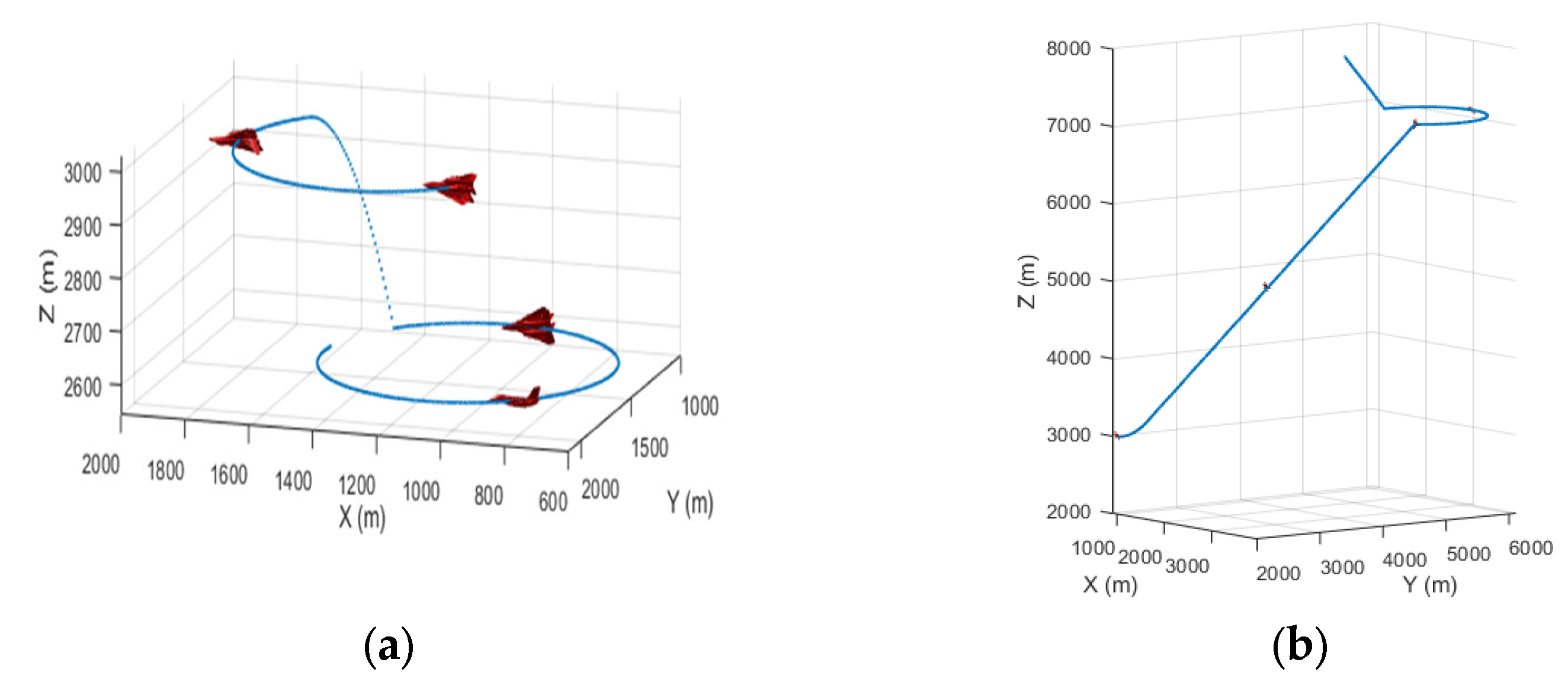
where M is the number of Monte Carlo simulations, X i j k is the i th component of the real state of the target at the k th moment of the j th simulation, and X i j k | k is the i th component of the state estimation vector at the k th moment of the j th simulation. These evaluation metrics enable component-wise analysis of the algorithm’s tracking performance across different dimensions. For the three-dimensional trajectory under investigation, we specifically evaluate position tracking accuracy along the X, Y, and Z axes of the Cartesian coordinate system, providing comprehensive spatial performance assessment. The simulation incorporates two distinct types of authentic UAV trajectories, as visually presented in Figure 7, allowing for clear observation of tracking effectiveness across all spatial dimensions.

4.2. Simulation Results and Discussion

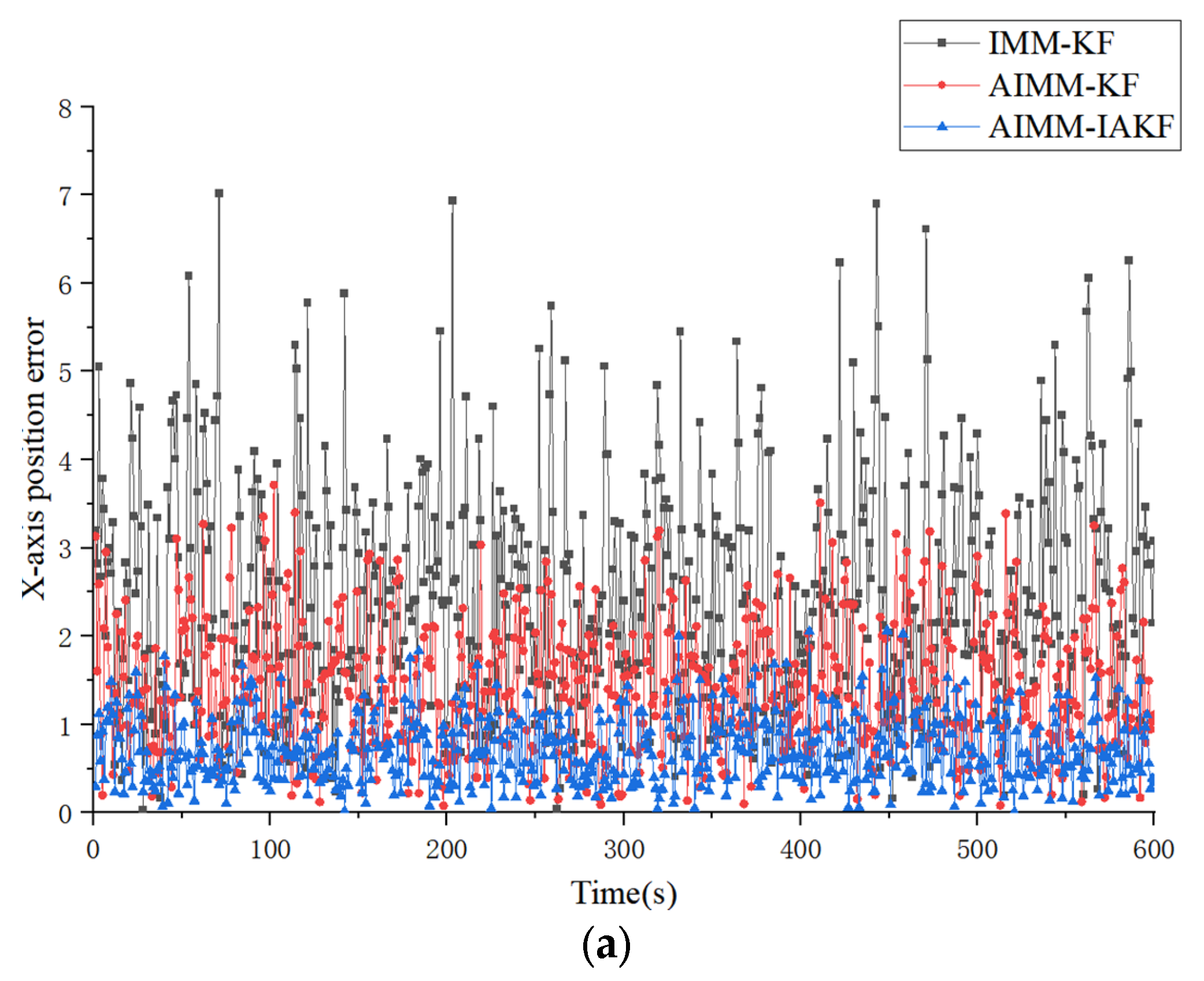
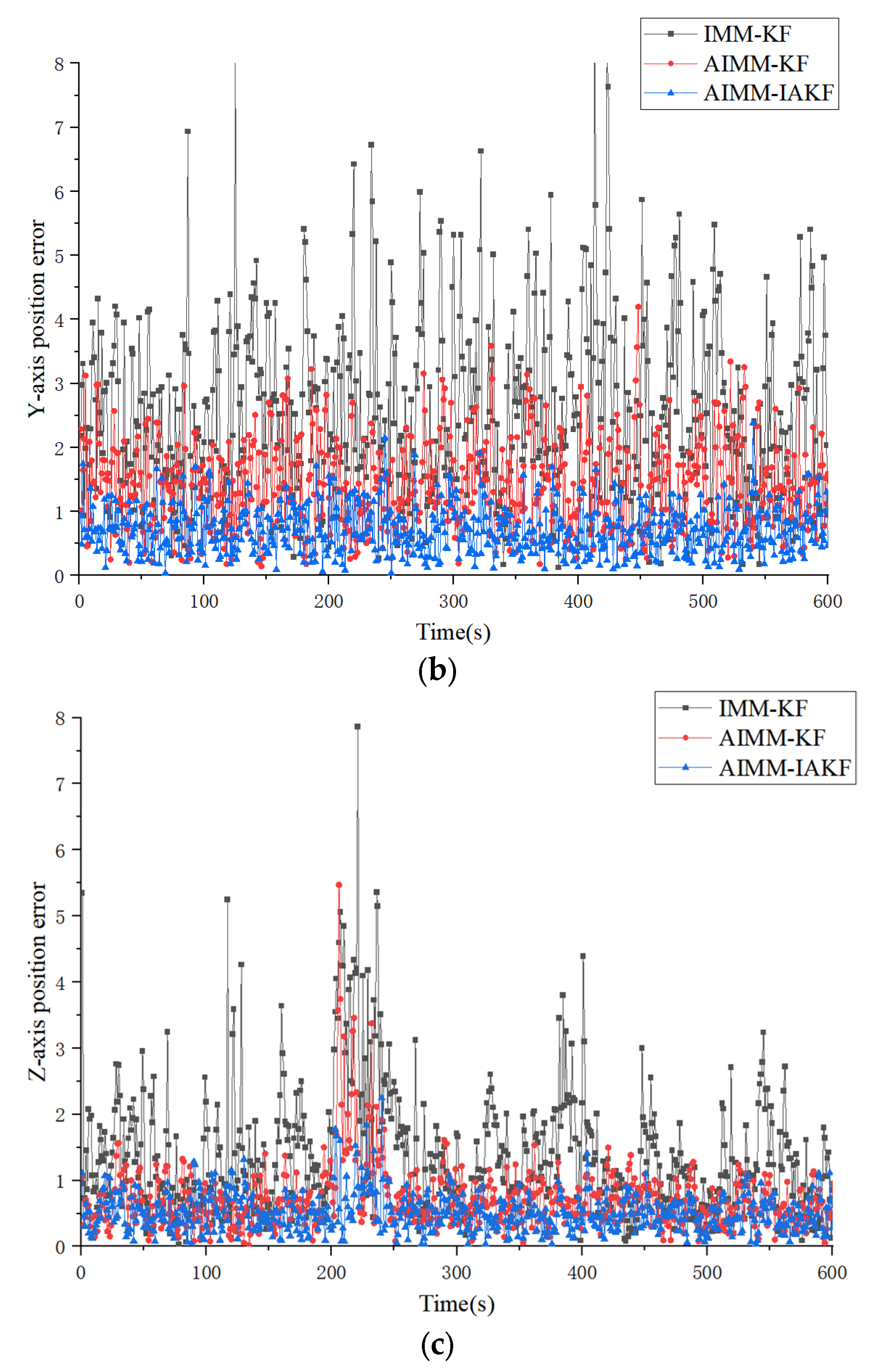
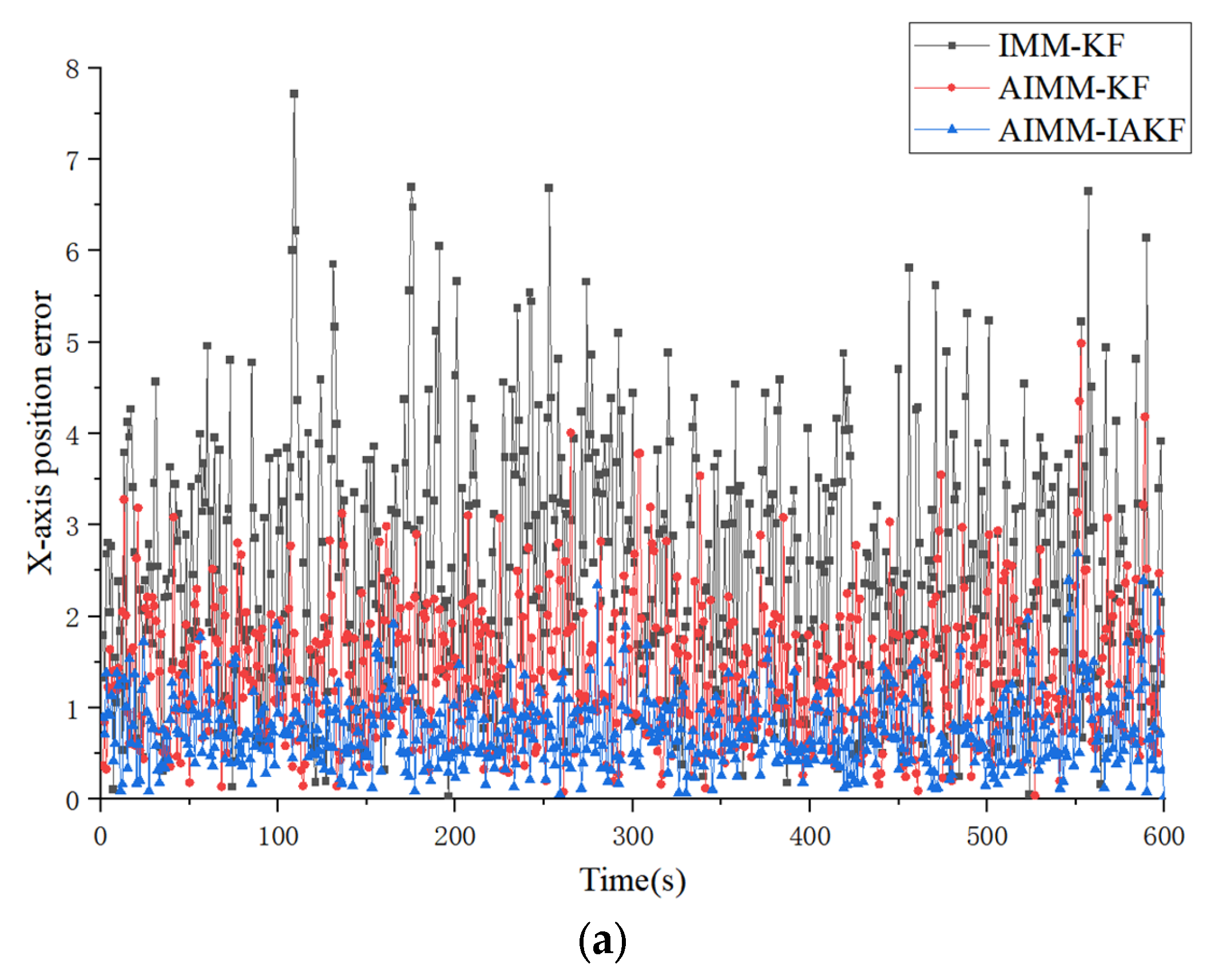
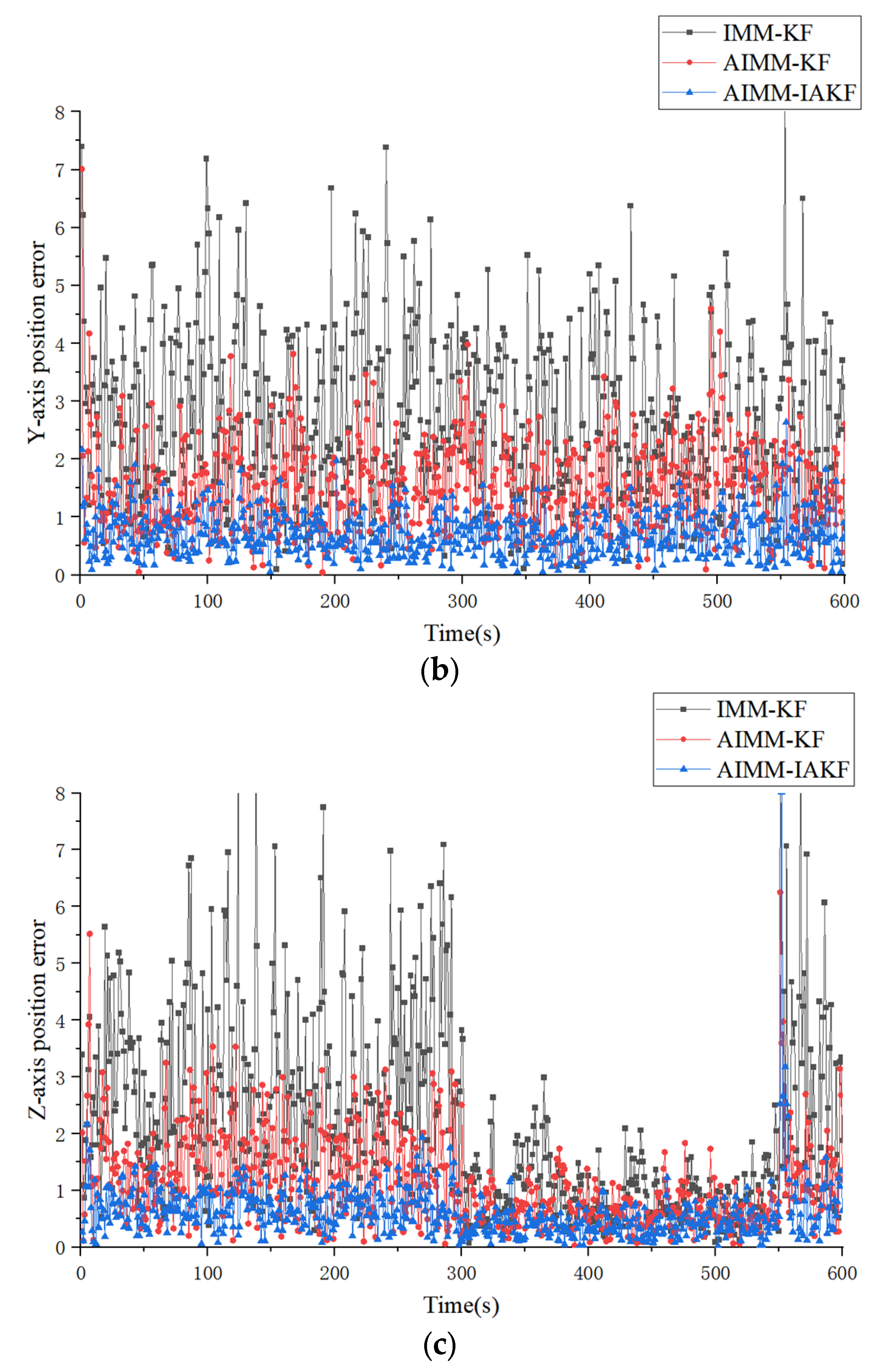
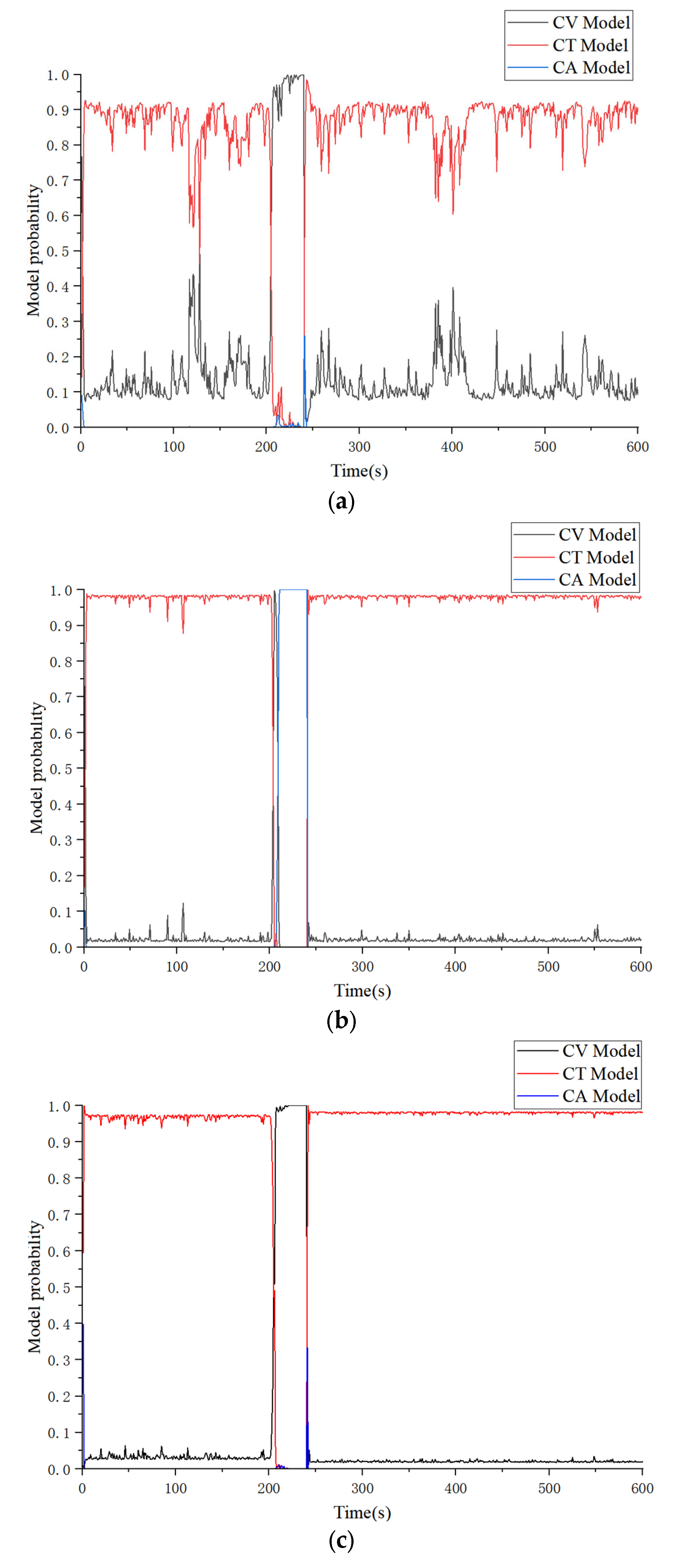
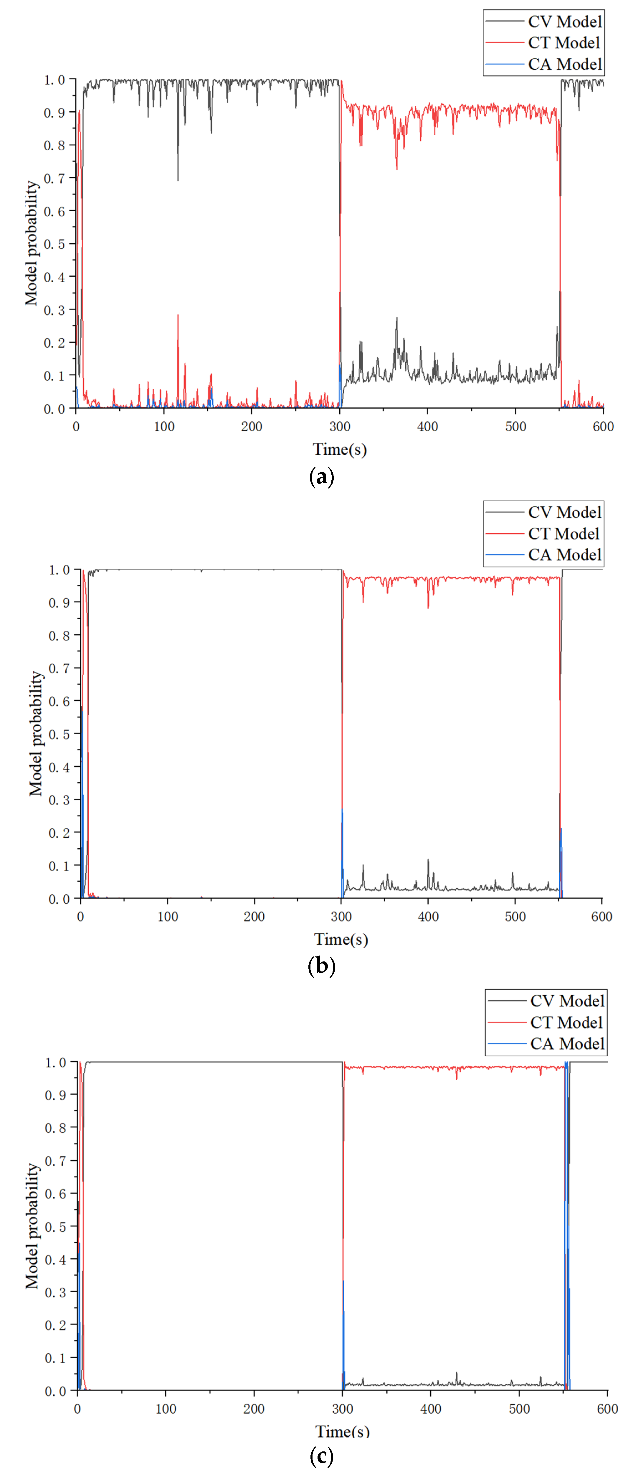
The study employs CV, CA, and CT as composite motion models to track both UAV types. For Type I UAVs, Figure 8 presents the RMSE in the X/Y/Z directions using the IMM-KF, Adaptive Interacting Multiple Model–Kalman Filter (AIMM-KF), and AIMM-IAKF algorithms, and the corresponding ARMSE results are summarized in Table 3. For Type II UAVs, Figure 9 presents the X/Y/Z directional RMSE, and the ARMSE results are summarized in Table 4. Furthermore, Figure 10 presents the model probability evolution for Type I UAVs, and Figure 11 presents the corresponding results for Type II UAVs.
Figure 8 and Figure 9 demonstrate that when tracking both UAV trajectories, the proposed AIMM-IAKF algorithm maintains consistently stable error bounds and achieves superior tracking accuracy overall. The AIMM-KF algorithm shows intermediate performance, while the conventional IMM-KF exhibits significantly larger error fluctuations, particularly along the Z-axis during CT model transitions, revealing its limited robustness in handling complex maneuvering patterns. These results indicate that the transition probability adjustment function significantly enhances adaptability and effectively reduces tracking errors, while the incorporation of IAKF further improves estimation accuracy by adaptively refining noise covariance updates.
Figure 10 and Figure 11 reveal significant improvements in model probability estimation across both UAV trajectories, demonstrating closer alignment with actual maneuvering patterns. The proposed AIMM-IAKF algorithm exhibits three key advantages over conventional IMM-KF and basic AIMM-KF approaches: (1) accelerated model switching response, (2) enhanced probability curve stability during steady-state tracking, and (3) near-ideal target model probability convergence (approaching 1). Clearly, the transition probability adjustment function effectively addresses the limitations of the fixed transition matrix in conventional IMM algorithms, leading to improved stability. Furthermore, the integration of IAKF further enhances tracking robustness and stabilizes model probability estimation under varying noise conditions.
The comparative results in Table 3 demonstrate that the proposed AIMM-IAKF algorithm achieves superior tracking performance, maintaining sub-meter ARMSE across all trajectory dimensions with minimal error fluctuations. In contrast, the conventional IMM-KF algorithm shows degraded performance, exceeding 1 m ARMSE in all directions. These simulation results confirm that the AIMM-IAKF algorithm provides significantly enhanced tracking stability and precision compared to traditional approaches.
The quantitative comparisons in Table 4 reveal three key findings: (1) The AIMM-KF algorithm improves tracking accuracy by approximately 45% over conventional IMM-KF through adaptive probability transition matrix adjustment, yielding significantly better model probability curves; (2) the AIMM-IAKF algorithm further enhances performance by 30% beyond AIMM-KF through suboptimal fading factor optimization and convergence criterion implementation, substantially boosting robustness and trajectory tracking precision; (3) combined, these advancements enable the AIMM-IAKF algorithm to achieve a remarkable 69% overall accuracy improvement compared to traditional IMM-KF methods.
A comparative analysis of computational performance was conducted. The average computation time per iteration for the IMM-KF, AIMM-KF, and AIMM-IAKF algorithms was found to be 13.2 ms, 13.8 ms, and 14.3 ms, respectively, on a standard desktop PC. As expected, the proposed AIMM-IAKF incurs a higher computational cost due to the adaptive mechanisms for both the transition matrix and noise statistics. However, the significant improvement in tracking accuracy justifies this cost for applications where precision is paramount. Furthermore, the convergence criterion in the IAKF component helps mitigate computational waste by preventing unnecessary covariance updates during steady-state conditions.

5. Conclusions

This paper presents an enhanced algorithm, AIMM–IAKF, which can be used to improve UAV trajectory tracking performance in complex and uncertain environments. The proposed approach integrates two key innovations. First, the AIMM component dynamically adjusts the model transition probability matrix by leveraging variations in transition probabilities between consecutive time steps, thereby overcoming the limitations of conventional IMM algorithms that rely on static matrices and expert-defined parameters. This adaptive mechanism enables faster model switching and improved tracking accuracy during rapid UAV maneuvers. Second, the conventional Kalman filter is replaced by an IAKF, which incorporates a suboptimal fading factor to optimize noise statistical characteristics and attenuate outdated covariance using historical data. A convergence criterion is further introduced to ensure computational efficiency while maintaining filtering stability. Simulation results demonstrate that the proposed AIMM–IAKF algorithm achieves approximately 69% improvement in tracking accuracy compared to the traditional IMM–KF method, along with faster model switching and superior stability across maneuvering scenarios.
While the algorithm has shown promising results in simulations, its performance necessitates validation with real UAV data, as inevitable gaps exist between simulation and real-world scenarios. Our model-based approach boasts training-free implementation and robust interpretability—attributes that hold significant value in practical applications. Moving forward, our primary focus will be on validating the algorithm using real UAV data to bridge the simulation–reality divide. Beyond this, we aim to explore hybrid architectures that incorporate machine learning strategies, with the goal of further enhancing tracking performance while preserving computational efficiency.

Author Contributions

Y.J. and C.L. were responsible for experimental implementation and manuscript writing. P.Z. provided academic guidance and comprehensive support during the research process. Z.W. and Y.L. undertook research supervision and manuscript revision. All authors have read and agreed to the published version of the manuscript.

Funding

This research was funded in part by a Shanxi Provincial Fundamental Research Program Grant under Grant 202103021224187 and TZLH20230818005. The Shanxi Province Graduate Student Practice and Innovation Program 2024SJ249 and, 2024KY628. Shanxi Science and Technology Innovation Leading Talent Team for Special Unmanned Systems and Intelligent Equipment 202204051002001.

Institutional Review Board Statement

Not applicable.

Informed Consent Statement

Not applicable.

Data Availability Statement

The data are available on reasonable request from the author.

Conflicts of Interest

The authors declare no conflicts of interest. Author Yunbiao Ji was employed by the company Chengdu Lingchuan Special Industrial Co., Ltd. The remaining authors declare that the research was conducted in the absence of any commercial or financial relationships that could be construed as a potential conflict of interest.

Nomenclature

SymbolDescription
XkSystem state vector at time k
ΦkState transition matrix
ZkMeasurement vector
HObservation matrix
Q, RSystem and measurement noise covariance matrices
KkKalman gain matrix
PkState estimation error covariance matrix
λkSuboptimal fading factor
εkInnovation (residual) sequence
μj(k)Probability of model j at time k
Π, pijModel transition matrix and its elements
αTransition probability adjustment speed parameter
TSampling interval
ωYaw rate
CVConstant Velocity model
CAConstant Acceleration model
CTConstant Turn model
IMMInteracting Multiple Model
KFKalman Filter
IAKFImproved Adaptive Kalman Filter
AIMMAdaptive Interacting Multiple Model
RMSERoot Mean Square Error
ARMSEAverage Root Mean Square Error

References

  1. Semenov, S.; Krupska-Klimczak, M.; Frontczak, M.; Yu, J.; He, J.; Chernykh, O. Adaptive Stochastic GERT Modeling of UAV Video Transmission for Urban Monitoring Systems. Appl. Sci. 2025, 15, 9277. [Google Scholar] [CrossRef]
  2. Yao, A.; Pal, S.; Li, G.; Li, X.; Zhang, Z.; Jiang, F.; Dong, C.; Xu, J.; Liu, X. FedShufde: A Privacy Preserving Framework of Federated Learning for Edge-Based Smart UAV Delivery System. Future Gener. Comput. Syst. 2025, 166, 107706. [Google Scholar] [CrossRef]
  3. Zhang, J.; Zhou, Z.; Huang, Q.; Liu, X.; Wang, B.; Hu, B. Real-Time Visual Monitoring and High Spatiotemporal-Resolution Mapping of Air Pollutants Using a Drone-Mass Spectrometer System. Environ. Sci. Technol. 2025, 59, 8099–8107. [Google Scholar] [CrossRef]
  4. Labib, N.S.; Brust, M.R.; Danoy, G.; Bouvry, P. The Rise of Drones in Internet of Things: A Survey on the Evolution, Prospects and Challenges of Unmanned Aerial Vehicles. IEEE Access 2021, 9, 115466–115487. [Google Scholar] [CrossRef]
  5. Ren, W.; Wei, Y.; Wang, C. Design of a Morphing Aircraft Based on Model Predictive Control. Appl. Sci. 2025, 15, 4380. [Google Scholar] [CrossRef]
  6. Shukla, P.; Shukla, S.; Singh, A.K. Trajectory-Prediction Techniques for Unmanned Aerial Vehicles (UAVs): A Comprehensive Survey. IEEE Commun. Surv. Tutor. 2024, 27, 1867–1910. [Google Scholar] [CrossRef]
  7. Savino, A. Multi-Fidelity Aerodynamic Optimization of the Wing Extension of a Tiltrotor Aircraft. Appl. Sci. 2025, 15, 9491. [Google Scholar] [CrossRef]
  8. Yuan, X.; Xu, J.; Li, S. Design and Simulation Verification of Model Predictive Attitude Control Based on Feedback Linearization for Quadrotor UAV. Appl. Sci. 2025, 15, 5218. [Google Scholar] [CrossRef]
  9. Kiciński, Ł.; Topczewski, S. Fuzzy Model Predictive Control for Unmanned Helicopter. Appl. Sci. 2025, 15, 8120. [Google Scholar] [CrossRef]
  10. Tkach, M. Trends in the Global Arms Market, Development of the Combat Drone Market: Impact and Consequences for Ukraine. Political Sci. Secur. Stud. J. 2023, 4. [Google Scholar] [CrossRef]
  11. Oprean, L.-G. Artillery and Drone Action Issues in the War in Ukraine. Sci. Bull. 2023, 28, 73–78. [Google Scholar] [CrossRef]
  12. Petrovski, A.; Delchev, G. Application of Drones with Artificial Intelligence for Military Purposes. In Proceedings of the 10th International Scientific Conference on Defensive Technologies (OTEH 2022), Belgrade, Serbia, 13–14 October 2022; pp. 92–100. [Google Scholar]
  13. Czarnecki, T.; Stawowy, M.; Kadłubowski, A. Cost-Effective Autonomous Drone Navigation Using Reinforcement Learning: Simulation and Real-World Validation. Appl. Sci. 2024, 15, 179. [Google Scholar] [CrossRef]
  14. Raj, A.; Ahuja, K.; Busnel, Y. AI Algorithm for Predicting and Optimizing Trajectory of Massive UAV Swarm. Robot. Auton. Syst. 2025, 186, 104910. [Google Scholar] [CrossRef]
  15. Carbone, M.R. When Not to Use Machine Learning: A Perspective on Potential and Limitations. MRS Bull. 2022, 47, 968–974. [Google Scholar] [CrossRef]
  16. Kalman, R.E. A New Approach to Linear Filtering and Prediction Problems. J. Basic Eng. 1960, 82, 35–45. [Google Scholar] [CrossRef]
  17. Wang, X.; Wang, A.; Wang, D.; Xiong, Y.; Liang, B.; Qi, Y. A Modified Sage-Husa Adaptive Kalman Filter for State Estimation of Electric Vehicle Servo Control System. Energy Rep. 2022, 8, 20–27. [Google Scholar] [CrossRef]
  18. Sun, D.; Yu, X.; Wang, C.; Zhang, C.; Huang, R.; Zhou, Q.; Amietszajew, T.; Bhagat, R. State of Charge Estimation for Lithium-Ion Battery Based on an Intelligent Adaptive Extended Kalman Filter with Improved Noise Estimator. Energy 2021, 214, 119025. [Google Scholar] [CrossRef]
  19. Zhang, J.; Zhou, W.; Wang, X. UAV Swarm Navigation Using Dynamic Adaptive Kalman Filter and Network Navigation. Sensors 2021, 21, 5374. [Google Scholar] [CrossRef]
  20. Fraser, C.T.; Ulrich, S. Adaptive Extended Kalman Filtering Strategies for Spacecraft Formation Relative Navigation. Acta Astronaut. 2021, 178, 700–721. [Google Scholar] [CrossRef]
  21. Jiang, L.; Wu, L. Enhanced Yolov8 Network with Extended Kalman Filter for Wildlife Detection and Tracking in Complex Environments. Ecol. Inform. 2024, 84, 102856. [Google Scholar] [CrossRef]
  22. Cheng, Y.; Zhang, S.; Wang, X.; Wang, H. Self-Tuning Process Noise in Variational Bayesian Adaptive Kalman Filter for Target Tracking. Electronics 2023, 12, 3887. [Google Scholar] [CrossRef]
  23. Sterpu, D.-A.; Măriuța, D.; Cican, G.; Larco, C.-M.; Grigorie, L.-T. Machine Learning Prediction of Airfoil Aerodynamic Performance Using Neural Network Ensembles. Appl. Sci. 2025, 15, 7720. [Google Scholar] [CrossRef]
  24. Singh, R.; Bhushan, B. Evolving Intelligent System for Trajectory Tracking of Unmanned Aerial Vehicles. IEEE Trans. Automat. Sci. Eng. 2022, 19, 1971–1984. [Google Scholar] [CrossRef]
  25. Urrea, C.; Agramonte, R. Kalman Filter: Historical Overview and Review of Its Use in Robotics 60 Years after Its Creation. J. Sens. 2021, 2021, 9674015. [Google Scholar] [CrossRef]
  26. Limaverde Filho, J.O.A.; Fortaleza, E.L.F.; Silva, J.G.; De Campos, M.C.M.M. Adaptive Kalman Filtering for Closed-Loop Systems Based on the Observation Vector Covariance. Int. J. Control 2022, 95, 1731–1746. [Google Scholar] [CrossRef]
  27. Akbaş, E.M.; Çifdalöz, O.; Üçüncü, M. Improving the Performance of a MEMS-IMU System Based on a False State-Space Model by Using a Fading Factor Adaptive Kalman Filter. Meas. Control 2024, 57, 1243–1251. [Google Scholar] [CrossRef]
  28. Cheng, Y.; Zhang, S.; Wang, X.; Wang, H.; Yang, H. Kalman Filter with Adaptive Covariance Estimation for Carrier Tracking under Weak Signals and Dynamic Conditions. Electronics 2024, 13, 1288. [Google Scholar] [CrossRef]
  29. Sun, B.; Zhang, Z.; Qiao, D.; Mu, X.; Hu, X. An Improved Innovation Adaptive Kalman Filter for Integrated INS/GPS Navigation. Sustainability 2022, 14, 11230. [Google Scholar] [CrossRef]
  30. Blom, H.A.P.; Bar-Shalom, Y. The Interacting Multiple Model Algorithm for Systems with Markovian Switching Coefficients. IEEE Trans. Automat. Contr. 1988, 33, 780–783. [Google Scholar] [CrossRef]
  31. Granstrom, K.; Willett, P.; Bar-Shalom, Y. Systematic Approach to IMM Mixing for Unequal Dimension States. IEEE Trans. Aerosp. Electron. Syst. 2015, 51, 2975–2986. [Google Scholar] [CrossRef]
  32. Zhao, B. Multisensor Maneuvering Target Fusion Tracking Using Interacting Multiple Model. Aut. Control Comp. Sci. 2024, 58, 303–312. [Google Scholar] [CrossRef]
  33. Wang, J.; He, J.; Peng, B.; Wang, G. Generalized Interacting Multiple Model Kalman Filtering Algorithm for Maneuvering Target Tracking under Non-Gaussian Noises. ISA Trans. 2024, 155, 148–163. [Google Scholar] [CrossRef] [PubMed]
  34. Yang, B.; Wang, H.; Shi, Z. Interacting Multiple Model Adaptive Robust Kalman Filter for Process and Measurement Modeling Errors Simultaneously. Signal Process. 2025, 227, 109743. [Google Scholar] [CrossRef]
  35. Xie, G.; Sun, L.; Wen, T.; Hei, X.; Qian, F. Adaptive Transition Probability Matrix-Based Parallel IMM Algorithm. IEEE Trans. Syst. Man Cybern, Syst. 2021, 51, 2980–2989. [Google Scholar] [CrossRef]
  36. Sun, M.; Duan, Q.; Xia, W.; Bao, Q.; Mao, Y. Multiple Adaptive Factors Based Interacting Multiple Model Estimator. IET Control Theory Amp; Appl 2024, 18, 1059–1069. [Google Scholar] [CrossRef]
  37. Lee, I.H.; Park, C.G. An Improved Interacting Multiple Model Algorithm with Adaptive Transition Probability Matrix Based on the Situation. Int. J. Control Autom. Syst. 2023, 21, 3299–3312. [Google Scholar] [CrossRef]
  38. Emambakhsh, M.; Bay, A.; Vazquez, E. Convolutional Recurrent Predictor: Implicit Representation for Multi-Target Filtering and Tracking. IEEE Trans. Signal Process. 2019, 67, 4545–4555. [Google Scholar] [CrossRef]
  39. Delande, E.; Houssineau, J.; Franco, J.; Frueh, C.; Clark, D.; Jah, M. A New Multi-Target Tracking Algorithm for a Large Number of Orbiting Objects. Adv. Space Res. 2019, 64, 645–667. [Google Scholar] [CrossRef]
  40. Mazor, E.; Averbuch, A.; Bar-Shalom, Y.; Dayan, J. Interacting Multiple Model Methods in Target Tracking: A Survey. IEEE Trans. Aerosp. Electron. Syst. 1998, 34, 103–123. [Google Scholar] [CrossRef]
  41. Yaacoub, J.-P.; Noura, H.; Salman, O.; Chehab, A. Security Analysis of Drones Systems: Attacks, Limitations, and Recommendations. Internet Things 2020, 11, 100218. [Google Scholar] [CrossRef]
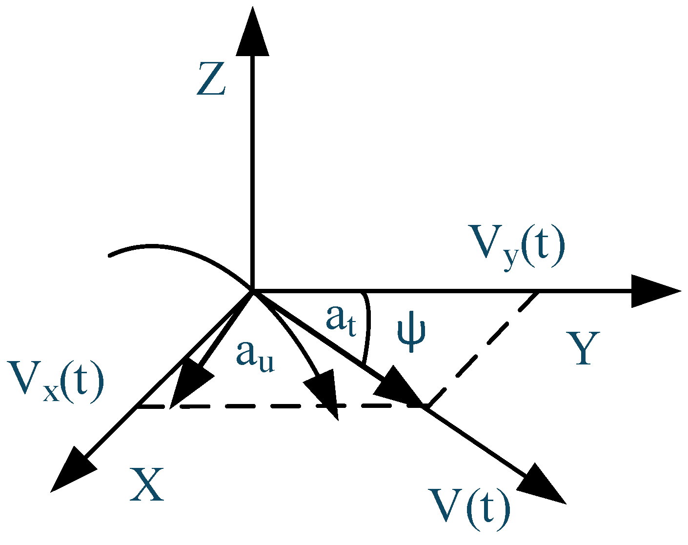
Figure 1. X-Y directions projection of CT model.
Applsci 15 11111 g001
Figure 2. Workflow diagram of UAV trajectory tracking based on the discrete-time Kalman filtering framework.
Applsci 15 11111 g002
Figure 3. Workflow diagram of UAV trajectory tracking based on the IAKF framework.
Applsci 15 11111 g003
Figure 4. Schematic diagram of IMM algorithm working principle.
Applsci 15 11111 g004
Figure 5. Schematic diagram of the improved adaptive IMM algorithm working principle.
Applsci 15 11111 g005
Figure 6. Workflow diagram of UAV trajectory tracking based on the AIMM-IAKF framework.
Applsci 15 11111 g006
Figure 7. Actual UAV trajectory diagrams: (a) Type I interceptor UAV trajectory; (b) Type II dive-bombing UAV trajectory.
Applsci 15 11111 g007
Figure 8. RMSE in X/Y/Z directions using IMM-KF, AIMM-KF, and AIMM-IAKF algorithms for Type I UAVs: (a) X-axis; (b) Y-axis; (c) Z-axis.
Applsci 15 11111 g008aApplsci 15 11111 g008b
Figure 9. RMSE in X/Y/Z directions using IMM-KF, AIMM-KF, and AIMM-IAKF algorithms for Type II UAVs: (a) X-axis; (b) Y-axis; (c) Z-axis.
Applsci 15 11111 g009aApplsci 15 11111 g009b
Figure 10. Model probability evolution for Type I UAVs trajectory tracking: (a) Model probability evolution of IMM-KF; (b) model probability evolution of AIMM-KF; (c) model probability evolution of AIMM-IAKF.
Applsci 15 11111 g010
Figure 11. Model probability evolution for Type II UAVs trajectory tracking: (a) Model probability evolution of IMM-KF; (b) model probability evolution of AIMM-KF; (c) model probability evolution of AIMM-IAKF.
Applsci 15 11111 g011
Table 1. Comparison of related work and proposed method.
MethodAdaptive Transition Matrix?Adaptive Noise Tuning?Key Limitation Addressed
Xie et al. [35]Yes (Correction Function)NoImproves switching but not filter robustness
Sun et al. [36]NoYes (Adaptive Factors)Wastes resources with stable noise
Lee et al. [37]Yes (Polarization Function)NoDoes not optimize noise characteristics
Proposed AIMM-IAKFYes (Exponential Adjustment)Yes (Fading Factor and Criterion)Simultaneously optimizes model switching and noise adaptation
Table 2. Simulation Parameters.
ParameterSymbolValueUnits
Sampling IntervalT1s
Total Sampling PointsN600-
Montecarlo RunsM100-
Initial State CovarianceP0100 · eye(9)-
System Noise Covariance (Initial)Qeye(3)m2
Measurement Noise Covariance (Initial)Rdiag([20, 20, 20])m2
Fading Factor Boundsλk[0.95, 0.995]-
Adjustment Speed Parameterα10-
Table 3. Tracking ARMSE for Two Types of Trajectories under Different Algorithms.
Algorithms & ModelsType of TrajectoryX-Axis (ARMSE/m)Y-Axis (ARMSE/m)Z-Axis (ARMSE/m)
IMM-KFType I2.9375842.9487841.648211
Type II2.6660032.7258562.333053
AIMM-KFType I1.4361441.4220950.711672
Type II1.3981131.5042591.126852
AIMM-IAKFType I0.7174120.7138910.507468
Type II0.7572250.7051260.612758
Table 4. Superiority of the Proposed Algorithms over Baselines in Terms of ARMSE Reduction.
ComparisonX-AxisY-AxisZ-Axis
Type IType IIType IType IIType IType II
AIMM-KF over IMM-KF51%48%52%45%56%52%
AIMM-IAKF over AIMM-KF50%46%50%52%30%46%
AIMM-IAKF over IMM-KF76%72%76%74%69%74%
Disclaimer/Publisher’s Note: The statements, opinions and data contained in all publications are solely those of the individual author(s) and contributor(s) and not of MDPI and/or the editor(s). MDPI and/or the editor(s) disclaim responsibility for any injury to people or property resulting from any ideas, methods, instructions or products referred to in the content.