Residual Life Prediction of SA-CNN-BILSTM Aero-Engine Based on a Multichannel Hybrid Network

Abstract

As the core component of an airplane, the health status of the aviation engine is crucial for the safe operation of the aircraft. Therefore, predicting the remaining service life of the engine is of great significance for ensuring its safety and reliability. In this paper, a multichannel hybrid network is proposed; this network is a combination of the one-dimensional convolutional neural network (1D-CNN), the bidirectional long short-term memory network (BiLSTM), and the self-attention mechanism. For each sensor of the engine, an SA-CNN-BiLSTM network is established. The one-dimensional convolutional neural network and the bidirectional long short-term memory network are used to extract the spatial features and temporal features of the input data, respectively. Moreover, multichannel modeling is utilized to achieve the parallel processing of different sensors. Subsequently, the results are stitched together to establish a mapping relationship with the engine’s remaining useful life (RUL). Experimental validation was conducted on the aero-engine C-MAPSS dataset. The prediction results were compared with those of the other seven models to verify the effectiveness of this method in predicting the remaining service life. The results indicate that the proposed method significantly reduces the prediction error compared to other models. Specifically, for the two datasets, their mean absolute errors were only 11.47 and 11.76, the root-mean-square error values were only 12.26 and 12.78, and the scoring function values were only 195 and 227.

1. Introduction

Aircraft engines, as the primary component of an aircraft, can have severe consequences in the event of a failure during flight [1]. To ensure flight safety, it is necessary to carry out predictive maintenance of aircraft engines, and predicting the remaining useful life (RUL) of aircraft engines is the key to implementing such maintenance. RUL prediction can provide important decision-making information for maintenance and reduce the maintenance costs of aircraft.

Currently, the mainstream methods for RUL prediction mainly fall into physical-based and data-driven models [2]. The approach based on physical failure models involves constructing a physical prediction model for RUL by integrating prior knowledge of the equipment composition, dynamics, and degradation mechanisms [3,4]. However, this method demands a substantial amount of prior learning. Moreover, it is challenging to build an accurate degradation model for highly complex systems such as aero-engines, leading to low prediction accuracy and limitations in application. In contrast, the data-driven prediction method for RUL extracts useful information from sensor-monitored parameters and employs data analytics to mine effective features to establish a mapping relationship with RUL. Subsequently, this relationship can be utilized to characterize the health of an aero-engine. This approach does not require much prior knowledge and can effectively handle the nonlinear relationship between degradation states and sensor data.

In data-driven approaches, deep learning-based prediction methods can directly model highly nonlinear, complex, and multidimensional systems and explore the mapping relationship between data and prediction goals. Babu et al. first used convolutional neural networks to predict the remaining life of an aero-engine [5]. Yu et al. utilized a combination of convolutional neural networks and long short-term memory networks to fully extract the data’s spatial and time features and predicted the remaining life of an aero-engine [6]. Li et al. used deep convolutional neural networks to extract the spatial properties of data in the time dimension by implementing deep convolutional operations along the time dimension of the sensor channel [7]. Guo et al. used recurrent neural networks (RNNs) to construct aero-engine health indicators and performed RUL using these health indicators [8]. Chen et al. proposed kernel global principal component analysis to extract the nonlinear features of sensor data, combined with gated recurrent units, to predict the RUL of an aero-engine [9]. To evaluate the RUL of an engine under complex operating conditions, Huang et al. developed an RUL prediction method based on a bidirectional long short-term memory network (Bi-LSTM) [10].

DULAIMI et al. predicted the RUL of an aero-engine using a hybrid approach combining a convolutional neural network and a bidirectional long short-term memory network, and the prediction accuracy of the hybrid model was significantly improved compared to the single model [11]. Ansari et al. constructed a multichannel artificial neural network (ANN) to extract multiple features of a battery, and their proposed model has a high degree of generalization [12]. Peng et al. proposed a prediction model with a parallel processing method [13]. Zhao et al. used a two-channel hybrid model to predict the RUL of an aero-engine, and the results showed that its performance was superior to that of the single-channel prediction model [14]. However, these methods cannot adequately extract effective information from sensor monitoring data. Thus, there is still room for improvement in prediction accuracy.

In this paper, to address the above problems, based on multichannel networks, a multichannel SA-CNN-BiLSTM RUL prediction method is proposed. This method targets one-dimensional time-series data from a single sensor, utilizes a 1D-CNN to mine the spatial features of the data, uses BILSTM to mine the temporal information of the data, and focuses on the useful information by using the self-attention mechanism, with each sensor monitoring parameter channel modeled individually to achieve parallel processing of different sensor data. For instance, regarding the vibration sensor data of an engine, a 1D convolutional neural network (1D-CNN) is capable of promptly capturing spatial characteristics, such as the amplitude and frequency of vibration signals within distinct time periods. Meanwhile, a bidirectional long short-term memory (BiLSTM) network analyzes the evolutionary trend of vibration features based on the time series. Moreover, the self-attention mechanism further concentrates on the crucial time periods and features that are tightly associated with the remaining life of the engine. This approach is expected to overcome the deficiencies of traditional methods and enhance prediction accuracy. Specifically, the self-attention mechanism places greater emphasis on the key periods and features relevant to the remaining life of the engine, with the aim of remedying the shortcomings of conventional approaches and improving the precision of predictions.

This paper initially elaborates on the architecture design of the multichannel SA-CNN-BiLSTM model, encompassing the specific functions and parameter settings of each layer within the network. It then describes in depth how the spatial and temporal characteristics of diverse sensor data can be comprehensively integrated. Subsequently, through experimental comparisons, real aero-engine monitoring data are employed to verify the superiority of the proposed model over traditional methods in terms of prediction accuracy, stability, and other aspects. Finally, the potential applications of this model, as well as the directions for future improvement, are summarized, offering novel ideas and approaches for the field of aero-engine residual life prediction. This, in turn, will contribute to enhanced aircraft flight safety and improved airline operational efficiency.

2. Basic Principles

2.1. Convolutional Neural Network

A convolutional neural network (CNN) is a multilayer feed-forward neural network. A typical CNN model consists of an input layer, convolutional layer, activation layer, pooling layer, fully connected layer, and output layer [15]. The convolutional and pooling layers are often arranged in an alternating pattern. The structure is shown in Figure 1, and the main functions of the layers are described in the following paragraphs.

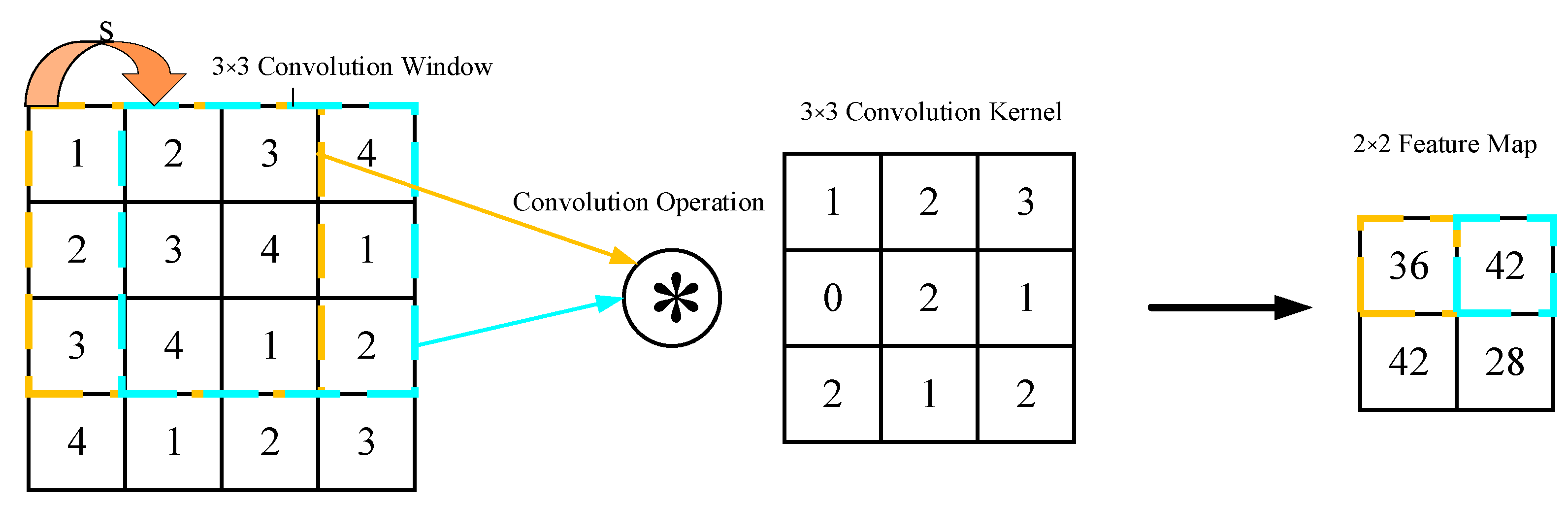
2.1.1. Convolutional Layer

The convolution kernel is the core of the convolutional layer for feature extraction. It extracts higher-order features by traversing the input data for convolutional operations. The convolutional layer is characterized by local awareness and weight sharing. That is, the weight matrix of the same convolution kernel is shared to reduce parameters and decrease model complexity. The convolution operation is shown in the following equation:

$$y_i^l\left(j\right)=w_i^{l-1} \ast x^{l-1}\left(j\right)+b_i^{l-1}$$

(1)

where $y_i^l\left(j\right)$ is the convolution result of layer $l$, $w_i^{l-1}$ is the weight matrix of layer $l-1$ (the weight matrix of the $i$th convolution kernel of layer $l-1$), and $x^{l-1}\left(j\right)$ denotes the $j$th region where the convolution operation is performed in layer $l-1$. $b_i^{l-1}$ denotes the bias term, which is the bias of the $i$th convolution kernel of layer $l-1$. The symbol $\ast$ denotes the convolution operation. The principle of the convolution kernel is shown in Figure 2.

The convolutional layer employs a predefined convolutional kernel to perform a local convolution on the input features in step s. After traversal, a feature map is generated. For instance, a 4 × 4 plane is computed by a 3 × 3 convolution kernel to obtain a 2 × 2 feature map. The parameters of the convolution kernel are multiplied with the corresponding parameters in the window and then summed to obtain the values in the feature map.

2.1.2. Activation Layer

In the forward propagation of a convolutional neural network, the activation layer nonlinearly transforms the output of the convolutional layer using an activation function. This maps low-dimensional, linearly indistinguishable features to higher dimensions and enhances the linear separability of the features. As a result, it enhances the nonlinear approximation and feature extraction capability of the neural network.

2.1.3. Pooling Layer

In a convolutional neural network (CNN), the pooling layer is designed to reduce computation by compressing the feature dimensions. It generalizes the higher-order features extracted by the convolutional layer, improves the network iteration efficiency, and endows the features with translation invariance. The common pooling methods include max pooling, which takes the maximum value in the perceptual domain, and average pooling, which takes the average value. The following formulas are used,

$$y_{i,j,k}^l=max\left\{x_{i,j,k}^l,s\right\}$$

(2)

$$y_{i,j,k}^l={\displaystyle \frac{1}{N}}\sum x_{i,j,k}^l$$

(3)

where $y_{i,j,k}^l$ is the $k$th feature map output in the $l$th layer, and $x_{i,j,k}^l$ is the $\left(i,j\right)$th element in the $k$th feature map output from the $l$th convolutional layer.

2.2. Bidirectional Long Short-Term Memory

The long short-term memory (LSTM) network, a recurrent neural network proposed by Hochreiter, overcomes the common gradient vanishing and explosion issues in recurrent neural networks (RNNs) [16]. An LSTM network can learn and retain sequential and temporal patterns in long sequences. Compared with traditional RNNs, LSTM networks depend on the gate mechanism and introduce forgetting, input, and output gates based on an RNN, controlling the information flow through the gate mechanism [17].

Bidirectional long short-term memory (BiLSTM) is an extension of the traditional long short-term memory (LSTM) network that improves the performance of the model in handling sequential problems. A BILSTM network structurally combines an LSTM network in both directions. Through its bidirectional structure, the output layer of the network can efficiently utilize the state information of the previous moment and that of the subsequent moment to make full use of the data for prediction. The structure of the model is shown in Figure 3. The BiLSTM network’s forward and backward layers process the sequences separately, and then the two outputs before and after are spliced to obtain the final output result. BiLSTM can be implemented using the following formulas:

$$\begin{gathered} \overrightarrow{h_t}=LSTM\left(\overrightarrow{h_{t-1}},x_t\right) \\ \overleftarrow{h_t}=LSTM\left(\overrightarrow{h_{t+1}},x_t\right) \\ {h}_t=\left[\overrightarrow{h_t},\overleftarrow{h_t}\right] \end{gathered}$$

(4)

where $h_t$ represents the output of the output layer at time $t$, $\overrightarrow{h_t}$ represents the output of the forward layer at time $t$, $\overleftarrow{h_t}$ represents the output of the backward layer at time $t$, and $x_t$ represents the input at time $t$.

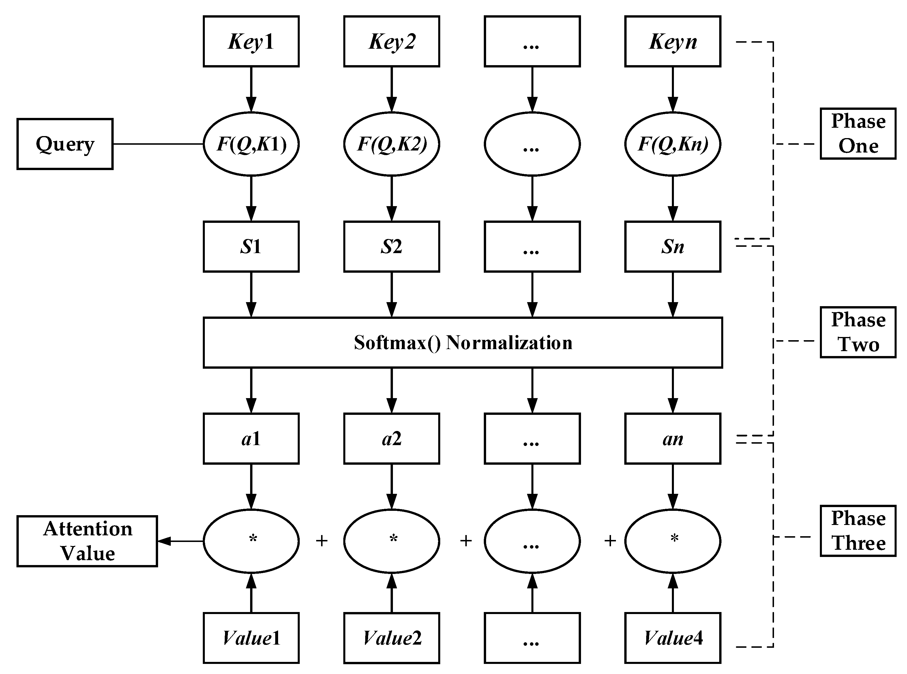
2.3. Attention Mechanism

The attention mechanism was first proposed in the field of machine vision. It imitates human vision and divides different regions with different weights to show the difference. The attention mechanism has been widely used in the field of deep learning in recent years due to its ability to strengthen key information and weaken invalid information. The calculation process for the attention mechanism can be divided into three stages, as shown in Figure 4.

In the first stage, the attention score corresponding to each key is obtained by calculating the similarity between the query and the key. In the second stage, the attention scores are normalized using the Softmax function to obtain the weighting coefficients. In the third stage, different weight coefficients are weighted and summed to highlight important information and ignore unimportant information. The formulas are shown below.

$$\begin{gathered} F\left(Q,K_i\right)=Q^T·K \\ {a}_i=softmax\left(F\left(Q,K_i\right)\right)={\displaystyle \frac{\exp \left(F\left(Q,K_i\right)\right)}{\sum _{i=1}^l\exp \left(F\left(Q,K_i\right)\right)}} \\ A\left(Q,K,V\right)=\sum _{i=1}^l{a}_i·V_i \end{gathered}$$

(5)

where $Q$ is the query matrix, $K$ is the key matrix, $V$ is the numerical matrix, and $a_i$ is the weight coefficient. When $Q=K=V$, the attention mechanism becomes a self-attention mechanism.

3. Multichannel SA-CNN-BiLSTM Network Model

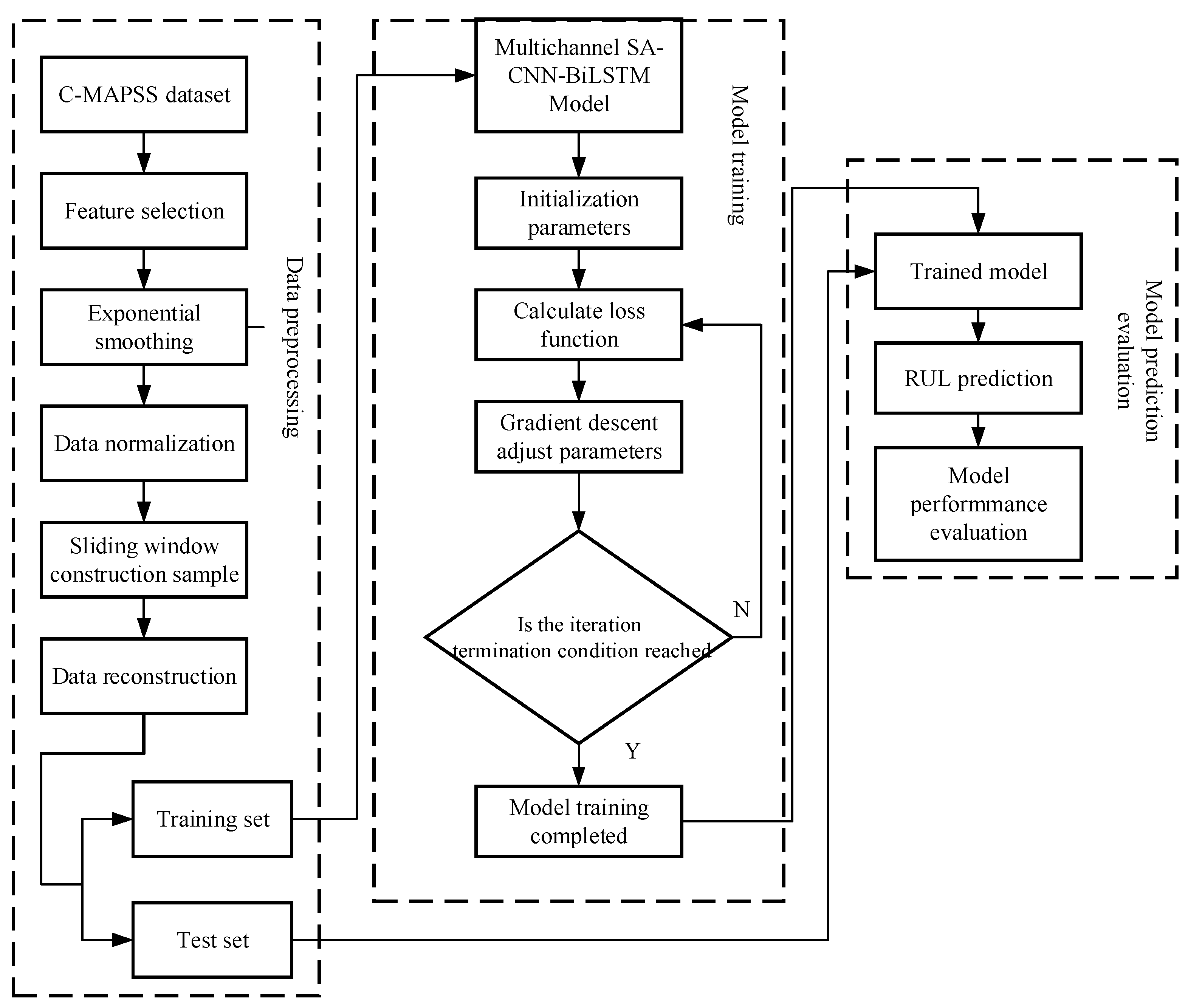
3.1. Remaining Life Prediction Model Training Prediction Process

Existing studies on the RUL prediction of aero-engines have used RNNs and CNNs as data-driven prediction methods, but CNNs cannot handle time-series signals efficiently and RNNs suffer from vanishing and exploding gradients. Here, a multichannel SA-CNN-BILSTM network model is proposed to predict the RUL of an aero-engine on a related basis. A separate channel is created for each sensor, with each channel containing two 1D-CNN layers and one BILSTM layer. The spatial features of the sensor data are extracted using the two 1D-CNN layers, and the extracted features are processed using the BILSTM layer with a time-demand process. Then, the extracted features are processed using the self-service network model. Time-demand processing is carried out, and then the self-attention mechanism is used to assign weights to the features and focus on the key information. The flow chart is shown in Figure 5.

3.2. Data Preprocessing

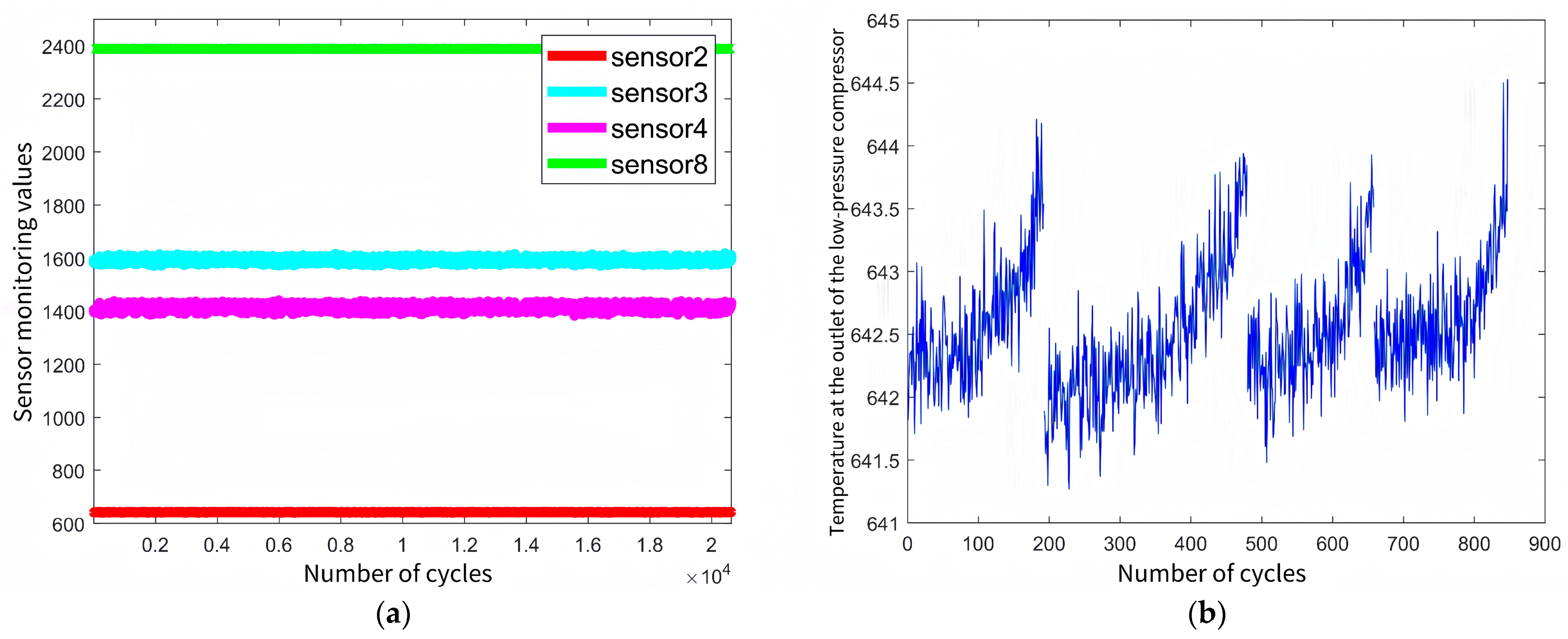
3.2.1. Data Pre-Description

The experimental data come from the degradation dataset of NASA’s C-MAPSS turbofan engine, a description of which is given in

Table 1. C-MAPSS sub-datasets.

Dataset	FD001	FD002	FD003	FD004
Operating conditions	1	6	1	6
Fault modes	1	1	2	2
Train trajectories	100	260	100	249
Test trajectories	100	259	100	248
Actual value of RUL	100	259	100	248

[18,19]. The data include four sub-datasets, from FD001 to FD004, each of which contains three files: the training set, the test set, and the true value of RUL.

The training and test sets consist of three operational parameters (altitude, Mach number, and sea level temperature) and 21 sensor parameters.

We evaluated the proposed method using the FD001 and FD003 datasets. It is worth noting that these two subsets correspond to specific operational conditions. For instance, the FD001 subset might cover data under a particular combination of altitude and Mach number, while the FD003 subset has its own distinct set of operating conditions and is unable to cover all operational scenarios. Nevertheless, their significance cannot be underestimated.

On the one hand, they offer a foundation for verifying the core algorithm of the prediction method and can assess the effectiveness of the model within specific scenarios. On the other hand, these specific scenarios are associated with high-frequency or critical operation phases in real life. The resultant model can provide direct support for the formulation of maintenance plans and the early warning of failures under the corresponding scenarios. Moreover, it can also serve as a crucial module for the construction of a comprehensive prediction system.

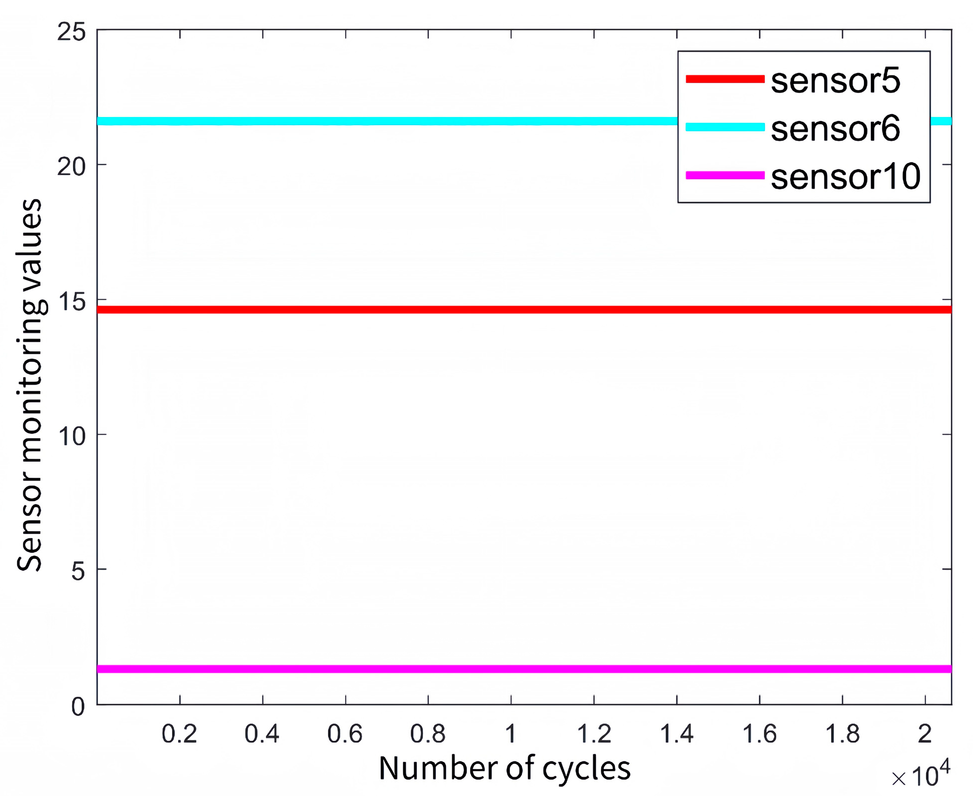
3.2.2. Feature Screening

Since not all sensor monitoring params can offer valuable info in model prediction, and excessive redundant data in the training set will increase training time and cause overfitting (as the model may learn too much noise, affecting prediction accuracy), it is crucial to filter out high-quality and valid data before RUL prediction to enhance model prediction performance.

Taking the FD001 dataset as an example, through visualizing the sensor data, certain representative data during a total of 20,631 cycle counts for 100 engines within the dataset are presented in Figure 6, Figure 7 and Figure 8.

Figure 6 illustrates the sensor data for the first type. The values of the monitoring information from sensors 5, 6, and 10 remained unchanged as the number of engine cycles increased. In total, this type of sensor encompasses seven sensors, namely sensors 1, 5, 6, 10, 16, 18, and 19. Since these sensors exhibited no variations in their values and failed to supply valid information during the model training process, these seven sensors were thus excluded.

Figure 7 depicts the second type of sensor data. On the whole, these data increased monotonically with the growth in the number of engine cycles for each engine. This type of sensor consists of a total of 10 sensors, namely No. 2–4, No. 8 and 9, No. 11, No. 13–15, and No. 17. Moreover, these sensors monitored the data in a cyclic manner to some extent.

Figure 8 illustrates the third type of sensor data. Overall, these data decreased monotonically with the increase in the number of engine cycles for each engine. This type of sensor encompasses a total of four sensors, namely No. 7, No. 12, and No. 20 and 21. Moreover, these sensors also exhibited a certain periodicity in their monitoring data.

With regard to the three types of sensor monitoring data mentioned above, the monitoring data of the first category of sensors remained constant as the number of cycles changed. From this, it can be inferred that this category of sensors did not incorporate information regarding the degradation of engine performance. Consequently, the seven sensors belonging to the first category were excluded. In contrast, the other two types of sensor data exhibited monotonic variations in tandem with the number of engine cycles. Hence, it can be assumed that they contain certain information related to performance degradation. Ultimately, the remaining 14 sensors were selected for the subsequent research work.

3.2.3. Data Normalization

Since the magnitudes of all 21 types of aero-engine sensor data vary, directly using these parameters for subsequent data processing and RUL prediction will cause bias in the prediction outcomes. Thus, in this study, the min–max function was used to normalize the sensor data. The normalization formula is as follows:

$$x_{i,j}^{*}={\displaystyle \frac{x_{i,j}-x_j^{min}}{x_j^{max}-x_j^{min}}}$$

(6)

where $x_j^{max}$ is the maximum value within the $j$th sensor, $x_j^{min}$ is the minimum value within the $j$th sensor, $x_{i,j}$ are the original data of the $j$th sensor at the $i$th moment, and $x_{i,j}^{*}$ are the data after normalization.

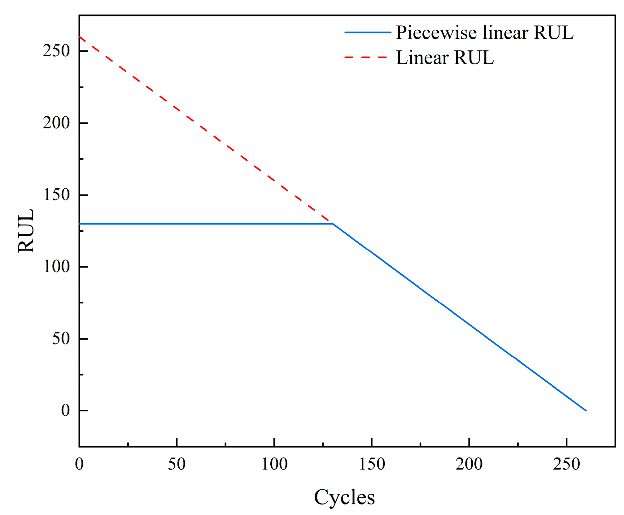
3.2.4. Segmented RUL Labeling

Taking into account that the operation data of the aero-engine manifest as a long time series, during the initial stage of operation, the engine performance remains relatively stable, and the degradation trend of the performance is not overly evident. Hence, it can be postulated that the value of the engine’s remaining useful life (RUL) will be maintained as a constant value within this specific period of time. When the operating time continuously increases and reaches the critical value $R$, the wear and tear of the components can no longer be overlooked. At this juncture, the remaining service life of the engine gradually diminishes along with the wear and aging of the hardware. Its RUL objective function is depicted in Figure 9.

To prevent the overestimation of the value of $R$, it is typically selected to be within the range of 55% to 65% of the average value of the engine running cycle. In this particular study, 65% was chosen, that is, $R=130$. When the number of engine running cycles amounted to fewer than 130, the remaining life of the engine gradually decreased as the engine operated. When the number of engine running cycles was greater than 130, the remaining life was set to a fixed value of $R$.

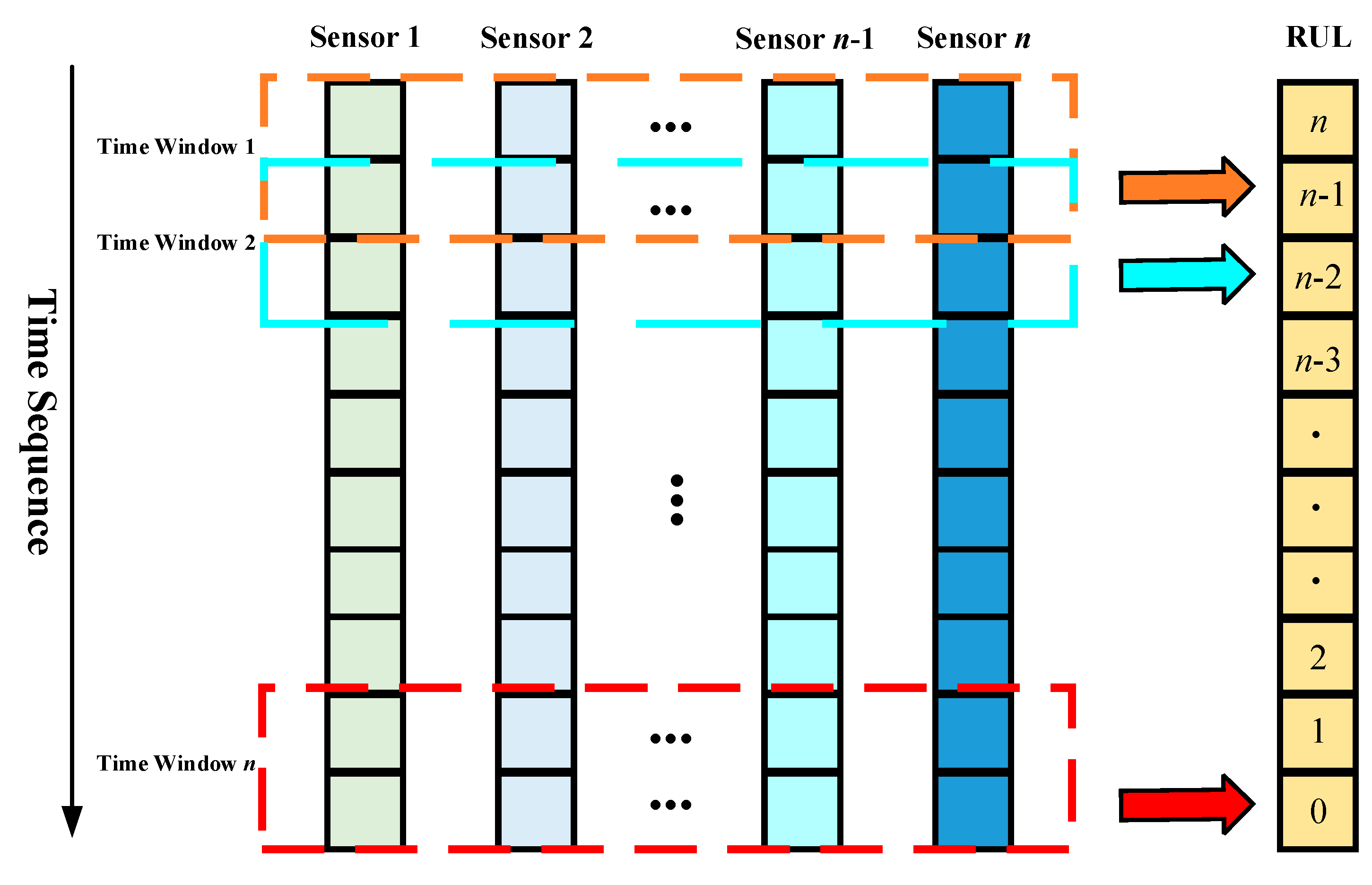
3.2.5. Sliding Time Window

In the context of time series, the quantity of features is closely associated with time. To avert the slow convergence of the model resulting from long sequences, a sliding time window is frequently employed to partition the data while simultaneously achieving data expansion. A schematic diagram of the sliding time window is presented in Figure 10. The size of the time window impacts the prediction performance. If the time window is too small, it becomes difficult to capture the correlation between the feature quantity and time promptly. Conversely, if the time window is too large, although more useful information will be encompassed, it is prone to overlooking short-term changes, thereby leading to insufficient learning.

4. Experimental Validation

4.1. Evaluation Criteria

To assess the precision and validity of the model prediction outcomes, three prevalently utilized metrics within the realm of aero-engine remaining useful life (RUL) prediction problems were chosen for evaluation in this paper, namely the mean absolute error (MAE), the root-mean-square error (RMSE), and the Score function (Score).

4.1.1. MAE

MAE (mean absolute error) is a statistical indicator used to measure the difference between predicted values and actual values. It calculates the average of the absolute values of the differences between predicted values and actual values. The formula is presented as follows:

$$MAE={\displaystyle \frac{1}{n}}\sum _{i=1}^n\left|y_i-\widetilde{y_i}\right|$$

(7)

where $n$ is the total number of test samples, and $y_i$ and $y_i$ are the true and predicted remaining useful life (RUL) values for the $i$th test sample data, respectively.

4.1.2. RMSE

The prediction of an aero-engine’s remaining useful life (RUL) is typically classified as a regression task. The root-mean-square error (RMSE) is a commonly employed evaluation metric in regression problems. The RMSE is utilized to gauge the disparity between the true value and the predicted value. The smaller the RMSE value, the more favorable the prediction performance of the model. Its calculation formula is presented as follows:

$$RMSE=\sqrt{{\displaystyle \frac{1}{n}}\sum _{i=1}^n{\left(y_i-\widetilde{y_i}\right)}^2}$$

(8)

where $n$ is the total number of test samples, and $y_i$ and $y_i$ are the true and predicted remaining useful life (RUL) values for the $i$th test sample data, respectively.

4.1.3. Score Evaluation Function

In real-world situations, the relationship between the true value and the predicted value holds crucial significance for the maintenance strategy. Early prediction enables timely maintenance; however, overly early prediction may result in a waste of resources. On the other hand, delayed prediction can give rise to safety hazards and substantial losses. The evaluation Score function makes up for the deficiencies of RMSE by imposing more stringent penalties on predicted values that are higher than the true values, thereby accurately assessing the prediction effect. The smaller the Score value, the better the prediction performance of the model. The formula is presented as follows:

$$Score=\left\{\begin{array}{c}{\displaystyle \sum _{i=1}^n}\left(e^{-{\displaystyle \frac{\widetilde{y_i}-y_i}{13}}}-1\right),\widetilde{y_i}-y_i<0\\ {\displaystyle \sum _{i=1}^n}\left(e^{-{\displaystyle \frac{\widetilde{y_i}-y_i}{10}}}-1\right),\widetilde{y_i}-y_i\ge 0\end{array}\right.$$

(9)

The Score function puts more emphasis on the lagged case by assigning higher penalty weights compared to the advance prediction.

4.2. Experimental Condition

The simulation environment was Intel Core i7-6700HQ, Windows 10, Python 3.8, and the backend is TensorFlow.

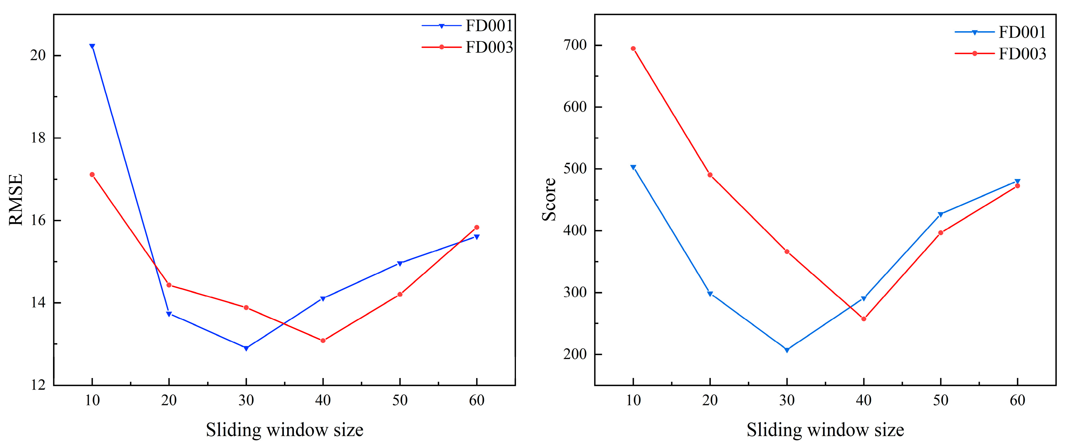
4.3. Analysis of Sliding Window Size Results

For long time series, the size of the sliding window constitutes an important parameter directly associated with the ultimate accuracy of a deep learning model. In this study, a sliding time window was introduced to reconstruct the 14-dimensional sensor data along with the remaining useful life (RUL) labeled data. 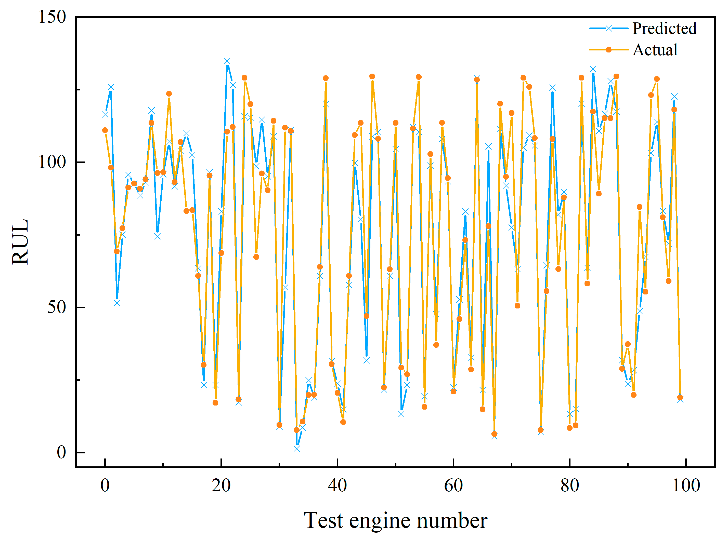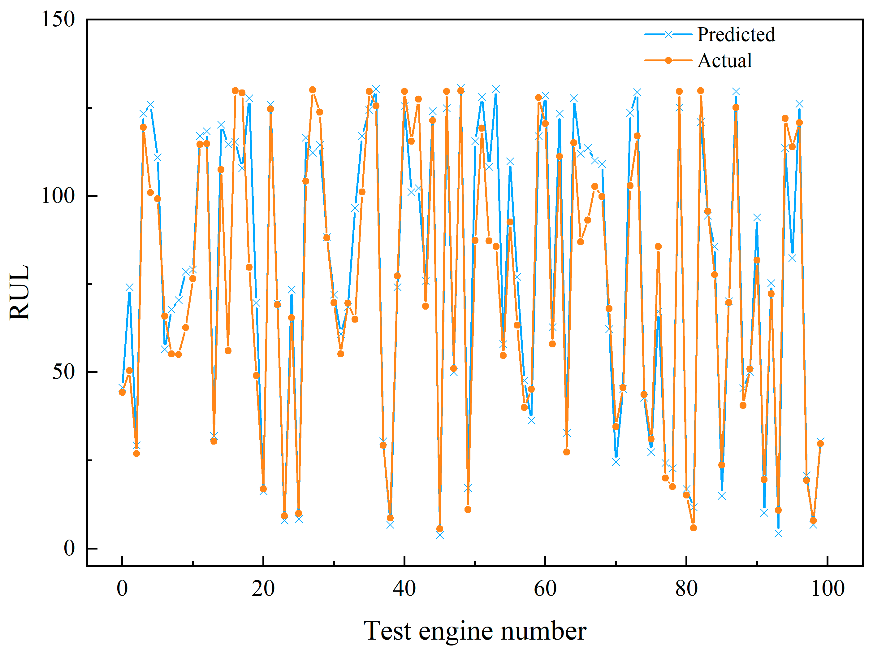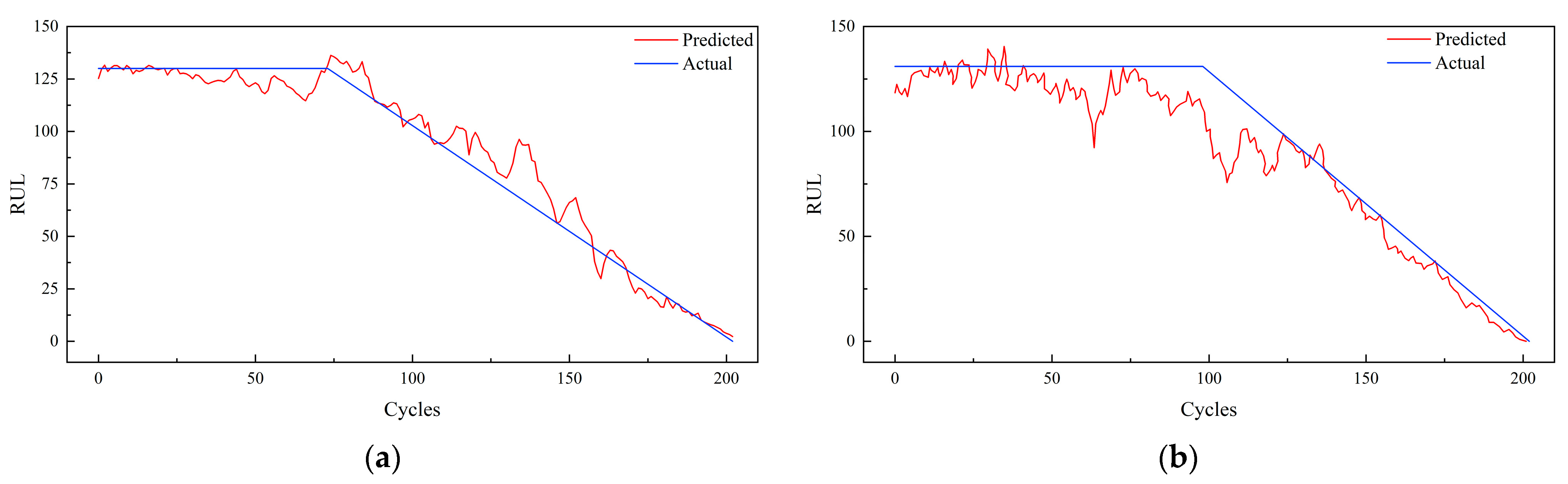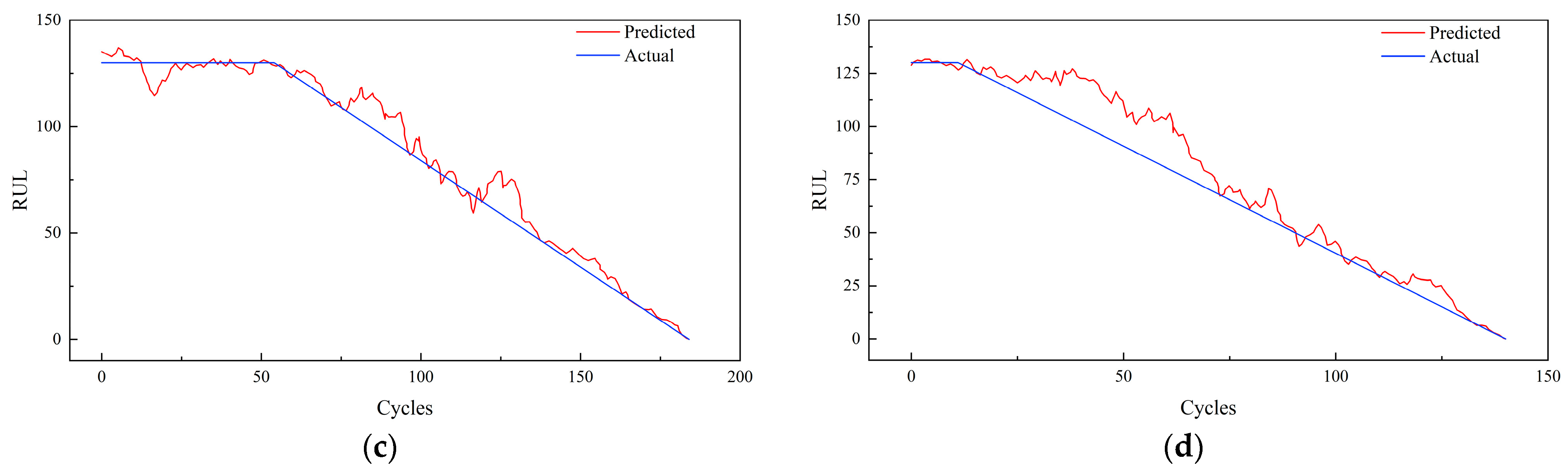To assess the impact of different window sizes on the accuracy of the prediction model, under an identical network structure, the window was set to sizes of 30, 40, 50, 60, 70, and 80, and the experimental results are presented in

Table 2. Effect of different sliding time window sizes on prediction results.

Window Sizes	FD001		FD003
	RMSE	Score	RMSE	Score
Lws = 10	20.2502	503.3330	17.1317	694.7253
Lws = 20	13.7231	298.7673	14.4360	490.3760
Lws = 30	12.9073	207.5724	13.8445	366.1153
Lws = 40	14.1324	291.1356	13.0865	257.3720
Lws = 50	14.9618	427.0348	14.2448	396.6330
Lws = 60	15.6623	480.7516	15.8343	472.5729

.

Figure 11 illustrates the impact of the sliding time window size within the aero-engine remaining life prediction model. As the window length expanded, the prediction effect gradually enhanced. However, when the window length surpassed 30 for the FD001 dataset and 40 for the FD003 dataset, the prediction performance exhibited a downward trend. Based on this finding, we opted to set the time window lengths of FD001 and FD003 to 30 and 40, respectively, thereby ensuring that the model attains high accuracy in predicting the remaining life of the aero-engine.

4.4. Analysis of Model Hyperparameter Results

To investigate the impact of the model’s hyperparameters on its prediction outcomes, this paper examines the effect of different hyperparameters on the prediction performance. The FD001 and FD003 datasets were tested separately, and the test results are presented in

Table 3. Effect of different model hyperparameter sizes on the prediction results.

Model Hyperparameters	FD001		FD003
	RMSE	Score	RMSE	Score
F = 32, K = 2	13.7407	135.9350	12.9706	267.9601
F = 64, K = 2	12.0347	67.5300	12.7825	194.5720
F = 32, K = 3	14.3873	154.2784	13.4312	278.8967
F = 64, K = 3	15.8711	170.6143	13.5116	345.2449

. The prediction results of the network model with different hyperparameters indicate that the optimal prediction results can be achieved when the number of filters (F) is set to 64 and the kernel size (K) is equal to 2.

4.5. Experimental Results and Analyses

The optimal model was employed to conduct tests on the FD001 and FD003 datasets, and its prediction results are presented in the following section. Additionally, for the purpose of attaining a more comprehensive understanding of the predicted engine degradation process, two engines were randomly chosen from each of the two sub-datasets, namely FD001 and FD003, to carry out engine prediction as well as the visualization and analysis of the actual degradation process. The results are displayed in Figure 12, Figure 13 and Figure 14.

From the prediction degradation process of the random test samples within the FD001 and FD003 test sets depicted in the above figure, it was observed that during the early stage of the test samples, the prediction value yielded by the proposed method was close to the set remaining useful life (RUL) threshold. Subsequently, the RUL prediction value generally decreased linearly with the operation time. Although there existed relatively large errors between the prediction value and the actual value at certain time points, when the engine operation approached the decommissioning stage, the accuracy of the prediction value was higher. This is because the later stages of the airline’s service period are of crucial importance for engine maintenance. A precise assessment of the engine state during this period can enhance the reliability and safety of operation and curtail maintenance costs.

Furthermore, to more effectively validate the efficacy of the proposed method, the prediction results of the proposed method were compared with those of other methods documented in the literature. The compared results are presented in

Table 4. Comparison of prediction results of different methods.

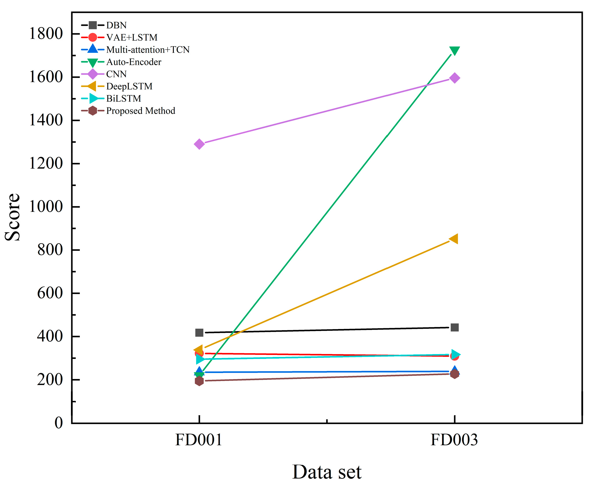
Method	FD001			FD003
	MAE	RMSE	Score	MAE	RMSE	Score
DBN [20]	13.46	15.21	418	12.74	14.71	442
VAE + LSTM [21]	14.14	15.88	322	12.25	14.29	309
Multi-attention + TCN [22]	12.16	13.25	235	11.96	13.43	239
Auto-Encoder [23]	12.48	13.58	220	16.28	19.16	1727
CNN [5]	16.12	18.45	1290	17.27	19.82	1596
DeepLSTM [24]	14.58	16.14	338	14.37	16.18	852
BiLSTM [25]	12.35	13.65	295	12.02	13.74	317
Proposed Method	11.47	12.26	195	11.76	12.78	227

.

Figure 15, Figure 16 and Figure 17 display a comparison of the results of the evaluation criteria under different methods. Observing these figures shows that the various network models attained good prediction results for the FD001 and FD003 datasets. Additionally, the remaining useful life (RUL) prediction model proposed in this chapter exhibited a significant improvement in prediction performance in comparison to the other network models. Concerning the prediction results for the FD001 dataset, when compared to the multi-attention + TCN method, which had the lowest mean absolute error (MAE) and root-mean-square error (RMSE), the MAE of the proposed method was reduced by 5.67%, the RMSE and Score of the proposed method were reduced by 7.47% and 17.02%, respectively. When contrasted with the Auto-Encoder method, which had the lowest Score, the MAE was reduced by 8.09%, the RMSE and Score decreased by 9.72% and 11.36%, respectively. As for the prediction results for FD003, in comparison to the multi-attention + TCN method, which exhibited the lowest MAE, RMSE, and Score, the MAE, RMSE, and Score of the proposed method were reduced by 1.67%, 4.84%, and 5.02%, respectively. The results of the two evaluation indexes, namely the MAE, RMSE, and Score, demonstrate that the prediction results of the method proposed in this paper are superior.

5. Conclusions

In this paper, an aero-engine remaining useful life (RUL) prediction model is put forward, which is based on the combination of a multichannel 1D convolutional neural network (CNN), bidirectional long short-term memory (BiLSTM), and a self-attention mechanism. Taking into account the data characteristics and analysis requirements, only the FD001 and FD003 subsets of the C-MAPSS dataset were utilized to construct and validate the proposed model in this research.

Regarding the model construction, a separate channel was established for each sensor to construct a model for feature extraction. A two-layer CNN was employed to process the monitoring data of the sensors, which enabled the effective extraction of spatial features. Subsequently, BiLSTM was adopted to ensure the extraction of time-series feature information. Meanwhile, with the assistance of the self-attention mechanism, the focus of the feature information was concentrated, endowing the model with a robust capability of capturing and analyzing features.

Nevertheless, it should be noted that the FD001 and FD003 subsets possess certain limitations. They represent specific operating conditions and are unable to cover all the operating scenarios of aero-engines. This may impact the generalizability of the model. When the model is applied to other scenarios, its performance may deviate from the current validation results. Hence, to improve the model, the validation scope needs to be expanded.

Despite the aforementioned limitations, the exploration conducted in this study based on specific subsets still offers valuable ideological and methodological references for the field of aero-engine RUL prediction and lays a certain foundation for the subsequent development of a more comprehensive and universal model.

References

- Chen, X.; Yu, J.; Tang, D.; Wang, Y. Remaining useful life prognostic estimation for aircraft subsystems or components: A review. In Proceedings of the IEEE 2011 10th International Conference on Electronic Measurement & Instruments, Chengdu, China, 16–19 August 2011; pp. 94–98. [Google Scholar]
- Nguyen, K.T.; Medjaher, K.; Tran, D.T. A review of artificial intelligence methods for engineering prognostics and health management with implementation guidelines. Artif. Intell. Rev. 2023, 56, 3659–3709. [Google Scholar] [CrossRef]
- Chiachío, J.; Jalón, M.L.; Chiachío, M.; Kolios, A. A Markov chains prognostics framework for complex degradation processes. Reliab. Eng. Syst. Saf. 2020, 195, 106621. [Google Scholar] [CrossRef]
- Shi, Y.; Zhu, W.; Xiang, Y.; Feng, Q. Condition-based maintenance optimization for multi-component systems subject to a system reliability requirement. Reliab. Eng. Syst. Saf. 2020, 202, 107042. [Google Scholar] [CrossRef]
- Sateesh Babu, G.; Zhao, P.; Li, X.-L. Deep convolutional neural network based regression approach for estimation of remaining useful life. In Database Systems for Advanced Applications, Proceedings of the Database Systems for Advanced Applications: 21st International Conference, DASFAA 2016, Dallas, TX, USA, 16–19 April 2016, Proceedings, Part I; Springer: Cham, Switzerland, 2016; pp. 214–228. [Google Scholar]
- Yu, S.; Wu, Z.; Zhu, X.; Pecht, M. A domain adaptive convolutional LSTM model for prognostic remaining useful life estimation under variant conditions. In Proceedings of the 2019 Prognostics and System Health Management Conference (PHM-Paris), Paris, France, 2–5 May 2019; pp. 130–137. [Google Scholar]
- Li, X.; Ding, Q.; Sun, J.-Q. Remaining useful life estimation in prognostics using deep convolution neural networks. Reliab. Eng. Syst. Saf. 2018, 172, 1–11. [Google Scholar] [CrossRef]
- Guo, L.; Li, N.; Jia, F.; Lei, Y.; Lin, J. A recurrent neural network based health indicator for remaining useful life prediction of bearings. Neurocomputing 2017, 240, 98–109. [Google Scholar] [CrossRef]
- Chen, J.; Jing, H.; Chang, Y.; Liu, Q. Gated recurrent unit based recurrent neural network for remaining useful life prediction of nonlinear deterioration process. Reliab. Eng. Syst. Saf. 2019, 185, 372–382. [Google Scholar] [CrossRef]
- Huang, C.-G.; Huang, H.-Z.; Li, Y.-F. A bidirectional LSTM prognostics method under multiple operational conditions. IEEE Trans. Ind. Electron. 2019, 66, 8792–8802. [Google Scholar] [CrossRef]
- Al-Dulaimi, A.; Zabihi, S.; Asif, A.; Mohammadi, A. A multimodal and hybrid deep neural network model for remaining useful life estimation. Comput. Ind. 2019, 108, 186–196. [Google Scholar] [CrossRef]
- Ansari, S.; Ayob, A.; Hossain Lipu, M.S.; Hussain, A.; Saad, M.H.M. Multi-channel profile based artificial neural network approach for remaining useful life prediction of electric vehicle lithium-ion batteries. Energies 2021, 14, 7521. [Google Scholar] [CrossRef]
- Peng, C.; Chen, Y.; Chen, Q.; Tang, Z.; Li, L.; Gui, W. A remaining useful life prognosis of turbofan engine using temporal and spatial feature fusion. Sensors 2021, 21, 418. [Google Scholar] [CrossRef]
- Zhao, C.; Huang, X.; Li, Y.; Yousaf Iqbal, M. A double-channel hybrid deep neural network based on CNN and BiLSTM for remaining useful life prediction. Sensors 2020, 20, 7109. [Google Scholar] [CrossRef] [PubMed]
- Heidelberg, S.B. Journal of Ambient Intelligence and Humanized Computing; Springer: Berlin/Heidelberg, Germany, 2023. [Google Scholar]
- Kawakami, K. Supervised Sequence Labelling with Recurrent Neural Networks. Ph.D. Thesis, Technical University of Munich, Munich, Germany, 2008. [Google Scholar]
- Gers, F.A.; Schraudolph, N.N.; Schmidhuber, J. Learning Precise Timing with LSTM Recurrent Networks. J. Mach. Learn. Res. 2003, 3, 115–143. [Google Scholar]
- Arias Chao, M.; Kulkarni, C.; Goebel, K.; Fink, O. Aircraft engine run-to-failure dataset under real flight conditions for prognostics and diagnostics. Data 2021, 6, 5. [Google Scholar] [CrossRef]
- Ramasso, E.; Saxena, A. Performance Benchmarking and Analysis of Prognostic Methods for CMAPSS Datasets. Int. J. Progn. Health Manag. 2014, 5, 1–15. [Google Scholar] [CrossRef]
- Zhang, C.; Lim, P.; Qin, A.K.; Tan, K.C. Multiobjective deep belief networks ensemble for remaining useful life estimation in prognostics. IEEE Trans. Neural Netw. Learn. Syst. 2016, 28, 2306–2318. [Google Scholar] [CrossRef]
- Su, C.; Li, L.; Wen, Z. Remaining useful life prediction via a variational autoencoder and a time-window-based sequence neural network. Qual. Reliab. Eng. Int. 2020, 36, 1639–1656. [Google Scholar] [CrossRef]
- Shang, Z.; Zhang, B.; Li, W.; Qian, S.; Zhang, J. Machine remaining life prediction based on multi-layer self-attention and temporal convolution network. Complex Intell. Syst. 2022, 8, 1409–1424. [Google Scholar] [CrossRef]
- Yu, W.; Kim, I.Y.; Mechefske, C. An improved similarity-based prognostic algorithm for RUL estimation using an RNN autoencoder scheme. Reliab. Eng. Syst. Saf. 2020, 199, 106926. [Google Scholar] [CrossRef]
- Zheng, S.; Ristovski, K.; Farahat, A.; Gupta, C. Long short-term memory network for remaining useful life estimation. In Proceedings of the 2017 IEEE International Conference on Prognostics and Health Management (ICPHM), Dallas, TX, USA, 19–21 June 2017; pp. 88–95. [Google Scholar]
- Wang, J.; Wen, G.; Yang, S.; Liu, Y. Remaining useful life estimation in prognostics using deep bidirectional LSTM neural network. In Proceedings of the 2018 Prognostics and System Health Management Conference (PHM-Chongqing), Chongqing, China, 26–28 October 2018; pp. 1037–1042. [Google Scholar]