Zero-TCE: Zero Reference Tri-Curve Enhancement for Low-Light Images

Abstract

Addressing the common issues of low brightness, poor contrast, and blurred details in images captured under conditions such as night, backlight, and adverse weather, we propose a zero-reference dual-path network based on multi-scale depth curve estimation for low-light image enhancement. Utilizing a no-reference loss function, the enhancement of low-light images is converted into depth curve estimation, with three curves fitted to enhance the dark details of the image: a brightness adjustment curve (LE-curve), a contrast enhancement curve (CE-curve), and a multi-scale feature fusion curve (MF-curve). Initially, we introduce the TCE-L and TCE-C modules to improve image brightness and enhance image contrast, respectively. Subsequently, we design a multi-scale feature fusion (MFF) module that integrates the original and enhanced images at multiple scales in the HSV color space based on the brightness distribution characteristics of low-light images, yielding an optimally enhanced image that avoids overexposure and color distortion. We compare our proposed method against ten other advanced algorithms based on multiple datasets, including LOL, DICM, MEF, NPE, and ExDark, that encompass complex illumination variations. Experimental results demonstrate that the proposed algorithm adapts better to the characteristics of images captured in low-light environments, producing enhanced images with sharp contrast, rich details, and preserved color authenticity, while effectively mitigating the issue of overexposure.

1. Introduction

Low-light image enhancement attracts considerable attention in optical target detection applications across diverse fields, including autonomous driving, military reconnaissance, and public safety, owing to its pivotal role in improving the accuracy and reliability of detection systems under challenging lighting conditions. However, during actual shooting in special scenarios like nighttime, severe weather conditions, or enclosed environments, high-quality images are often unobtainable due to external natural factors and the limitations of shooting equipment [1]. The captured images frequently exhibit low contrast, blurred details, and color distortion [2], making it difficult to distinguish between targets and backgrounds. Furthermore, target edges and texture features are weakened, and noise interference is significantly increased, severely impacting the accuracy of optical target detection. Hence, the enhancement of low-light images is indispensable for ensuring optimal performance in various applications.

The primary task of low-light image enhancement is to improve image visibility and contrast [3,4], while simultaneously addressing complex degradation patterns such as noise, artifacts, and color distortion introduced by brightness enhancement. Researchers have introduced a multitude of algorithms for enhancing low-light images, which can be comprehensively categorized into three distinct groups: those grounded in traditional image processing theory, those built upon physical models, and those leveraging advanced deep learning techniques. Among them, algorithms grounded in traditional image theory focus on improving image quality by adjusting image grayscale values. They primarily encompass classic traditional image enhancement techniques such as histogram equalization [5,6], gradient domain methods [7], homomorphic filtering [8], and image fusion [9]. Histogram equalization enhances contrast through the redistribution of pixels, with main approaches including standard histogram equalization (HE) [10], adaptive histogram equalization (AHE) [11], and contrast-limited adaptive histogram equalization (CLAHE) [12]. However, these methods largely ignore illumination factors, potentially leading to over-enhancement, artifacts, and unexpected local overexposure [13]. Gradient domain image enhancement algorithms are generally limited to the enhancement of single images or images captured in the same scene [14]. Meanwhile, homomorphic filtering algorithms enhance the high-frequency details of an image by attenuating its low-frequency components, but the cutoff frequency is not fixed and requires extensive experimentation based on specific images.

Algorithms for enhancing low-light images based on physical models process these images by simulating the imaging principles of the human visual system. They primarily encompass the following two approaches: First, algorithms based on the Retinex theory [15], including Single-Scale Retinex (SSR) [16,17], Multi-Scale Retinex (MSR) [18], and Multi-Scale Retinex with Color Restoration (MSRCR), are utilized [19]. These algorithms leverage human visual color constancy, simulating the human eye’s perception mechanism of object colors, to separate color images into illumination and reflection components, thereby effectively enhancing the images. Such algorithms perform well in terms of illumination invariance, but if noise and other factors are not carefully considered, they may lead to unrealistic images or localized color distortions. To address this issue, Kimmel et al. [20] transformed the approximate illumination problem into a quadratic programming problem to find an optimal solution, which improved the enhancement effect of low-light images to a certain extent. Wang et al. [21] refined the Retinex algorithm by incorporating nonlocal bilateral filtering into the luminance component within the HIS color space. By subtracting the resultant image, via post-Laplacian filtering, from the original image, they achieved commendable enhancement results. However, this approach inadvertently introduced noise and resulted in some degree of edge blurring. Ji et al. [22] used guided filtering to estimate the illumination of the image’s luminance component and used combined gamma correction [23] to adjust the incident and reflection components. This reserved the image’s colors to a certain extent but still resulted in an overall darker image. Second, the atmospheric scattering model is utilized to defog inverted low-light images. This method leverages the similarity between inverted low-light images and hazy images, integrating prior knowledge, such as the dark channel prior [24], to effectively eliminate haze from the image and consequently enhance the quality of the low-light image. Dong et al. [25] introduced an innovative algorithm, grounded in the atmospheric scattering model, to directly apply channel-wise prior dehazing techniques after inverting the low-light images. However, this algorithm introduces excessive noise, making the overall image appear unnatural. Li et al. [26] used Block Matching and 3D filtering (BM3D) [27] for denoising in order to separate the base layer and enhancement layer of the image, adjusting each layer separately to achieve better results. These methods have achieved certain effects in low-light image enhancement, but they lack a physical basis and may introduce excessive noise, resulting in a certain degree of blurring and making the overall image appear unnatural.

In recent years, with the surge of interest in deep learning, several deep learning models have emerged that are tailored for low-light image enhancement. Existing deep learning models can be broadly categorized into supervised and unsupervised types. Supervised learning models are designed to automatically discern and learn the intricate mapping relationship between low-light and normal-light images. By deeply analyzing and exploring the inherent characteristics of low-light images, these models are capable of achieving high-quality image enhancement and restoration. Hu et al. [28] proposed the Pyramid Enhancement Network (PE-Net), utilizing a Detail Processing Module (DPM) to enhance image details and validate the algorithm’s utility in nighttime object detection tasks in conjunction with YOLOv3. Liu et al. [29] introduced a Differentiable Image Processing (DIP) module to improve the object detection performance under adverse conditions, enhancing images through a weakly supervised approach for object detection. This enabled adaptive image processing under both normal and unfavorable weather conditions, albeit with limited image enhancement effects. Kalwar et al. [30] introduced a pioneering Gated Differentiable Image Processing (GDIP) mechanism, which facilitated the concurrent execution of multiple DIP operations, thereby enhancing the efficiency and flexibility of image processing tasks. Inspired by the Retinex theory, Wei et al. [31] presented RetinexNet, which achieved remarkable results under low-light conditions but exhibited limitations in processing color information and edge details, resulting in blurred edge areas and distorted edge details during the smooth denoising of the reflectance image. To address color deviation issues, Cai et al. [32] introduced Retinexformer, composed of illumination estimation and image restoration, using an illumination-guided Transformer in order to suppress noise and color distortion. However, this algorithm failed to balance brightness adjustment between bright and dark areas, easily causing overexposure in the originally brighter regions of the image. Zhang et al. [33] established the KinD++ network, which not only enhanced the brightness of dark areas but also effectively removed artifacts by separately adjusting illumination and removing degradation in the reflectance map.

Unsupervised deep learning models, which do not require labeled data, exhibit strong generalization capabilities. However, due to the lack of direct supervision, their enhancement effects may be less stable. Drawing upon the principles of the Retinex theory, Zhang et al. [34] devised a novel Generative Adversarial Network (GAN) approach that did not necessitate the use of paired datasets. This method achieves remarkable low-light image enhancement through the judicious utilization of controlled discriminator architectures, self-regularized perceptual fusion techniques, and sophisticated self-attention mechanisms. Yet, due to the neglect of physical principles, artifact phenomena can easily arise. Subsequently, Shi et al. [35] presented the RetinexGAN network, a sophisticated framework that is meticulously divided into two distinct components for image decomposition and enhancement. However, it is noteworthy that an overemphasis on distribution during the enhancement process may inadvertently result in unnatural-looking enhanced images. Jiang et al. [36] proposed an efficient unsupervised generative adversarial network (EnlightGAN), which utilizes an unsupervised generative adversarial network combined with an attention-guided U-Net generator and a global–local discriminator to enhance low-light images, demonstrating good domain adaptability. Liang et al. [37] introduced an innovative unsupervised backlit image enhancement technique, CLIP-LIT. This method leverages the robust capabilities of the CLIP model and achieves the effective enhancement of backlit images through a prompt learning framework and iterative fine-tuning strategies. However, it is worth noting that this method relies on a pre-trained CLIP model and may fail in some extreme cases, such as when information is missing in overexposed or underexposed areas. Yang et al. [38] pioneered the utilization of the controllable fitting capability of neural representations, proposing an implicit neural representation method named NeRCo for low-light image enhancement, which demonstrates exceptional performance in restoring authentic tones and contrast. Chobola et al. [39] presented an algorithm that reconstructs images in the HSV space using implicit neural functions and embedded guided filtering, effectively improving image quality and scene adaptability, although overexposure can still occur in highlight areas. Guo et al. [40] converted low-light image enhancement into a deep curve estimation problem, proposing a zero-reference deep curve estimation (Zero-DCE) network. By setting a series of reference-free loss functions, the network achieves end-to-end training without any reference images. Although brightness is significantly improved, contrast remains low, and processing directly on the RGB channels of the image can easily lead to color distortion. Li et al. [41] improved upon this by proposing Zero-DCE++, which uses downsampling to input images and learn mapping parameters, followed by upsampling and final image processing with the learned parameters to enhance low-light images. This results in good performances in color preservation and overall smoothness, but may cause overexposure in originally well-exposed areas. Compared with traditional algorithms, deep learning algorithms have more stringent data requirements, and low-light images typically suffer from poor quality, with minimal differences between targets and backgrounds. This leads to the ineffective enhancement of dark areas by deep learning algorithms and insufficient robustness.

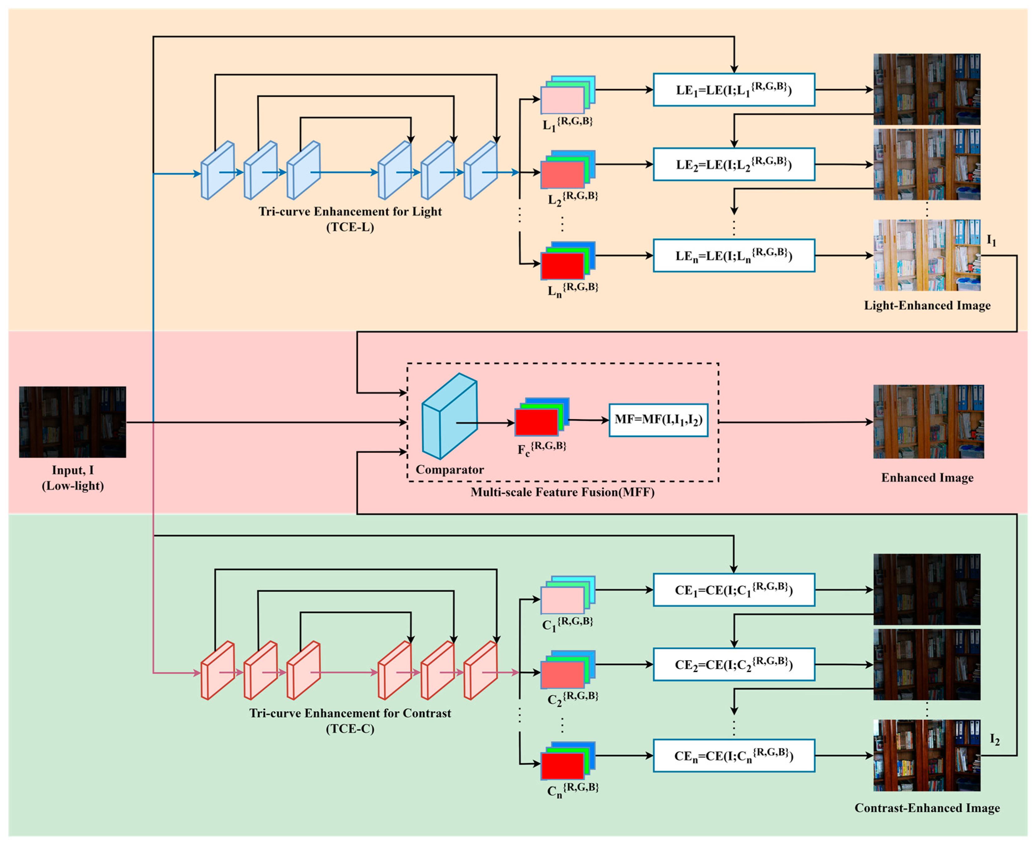
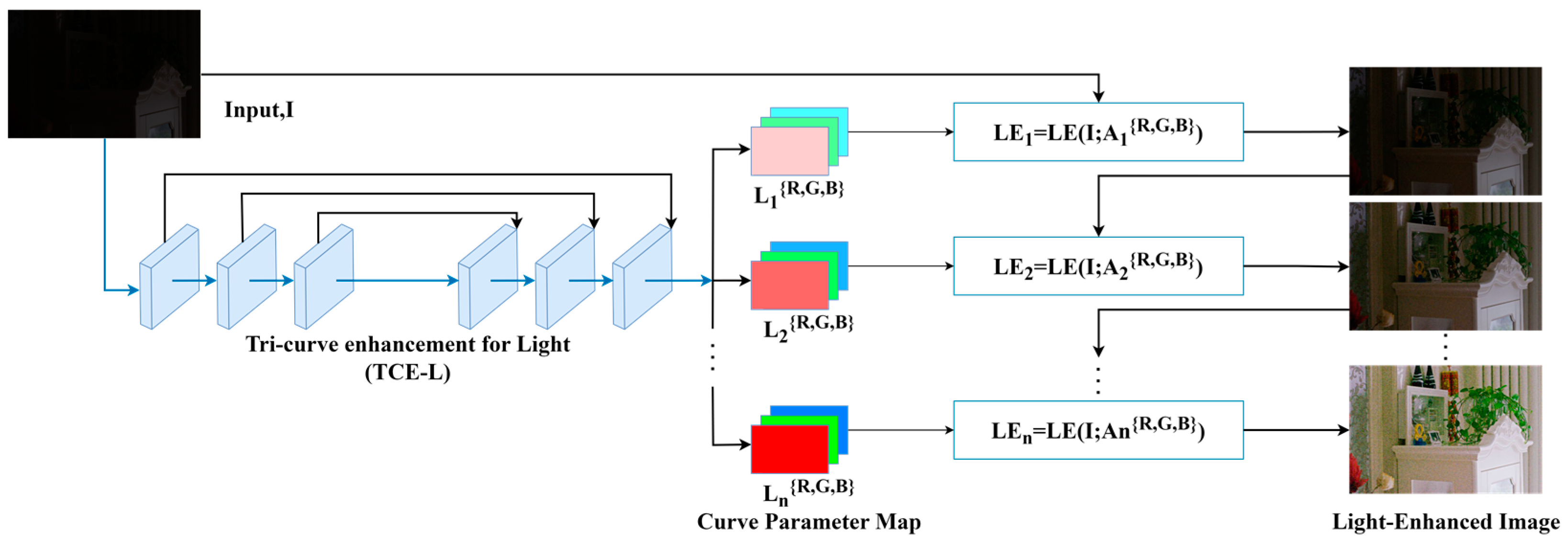
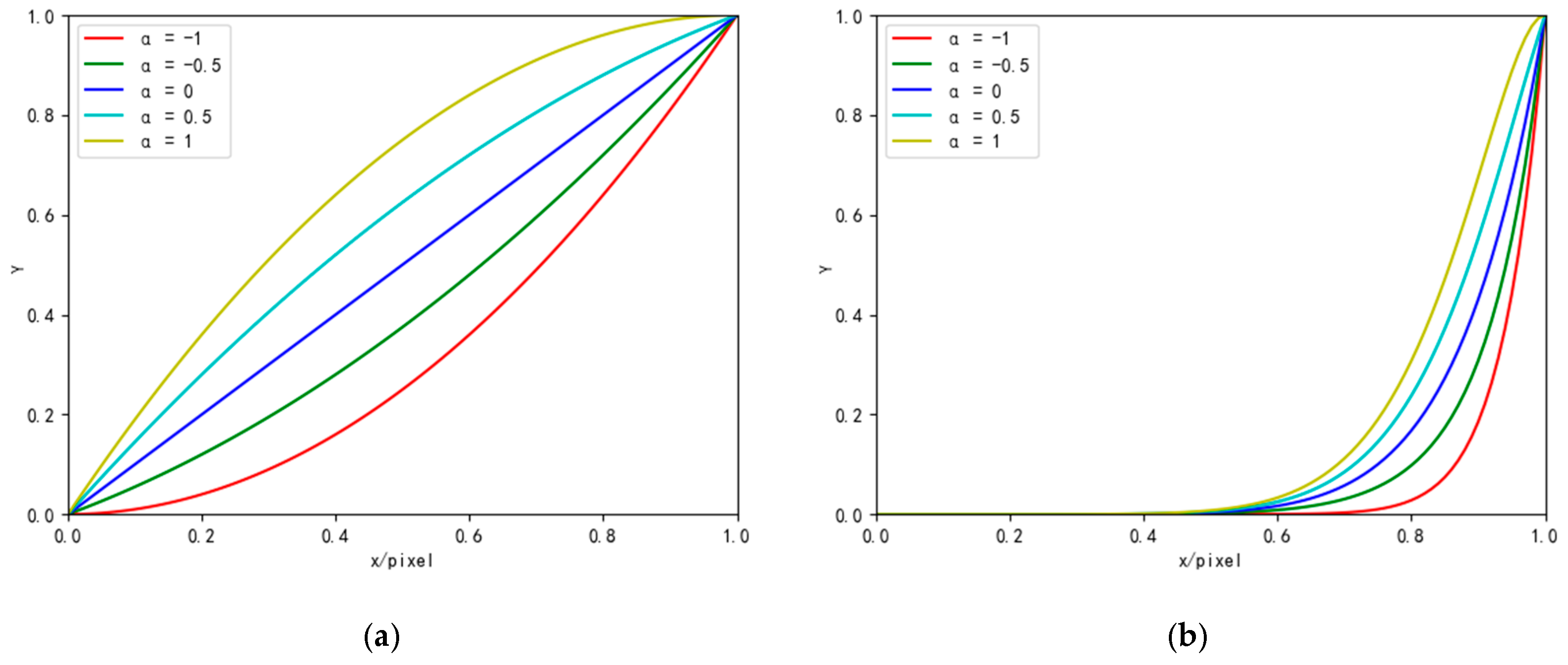
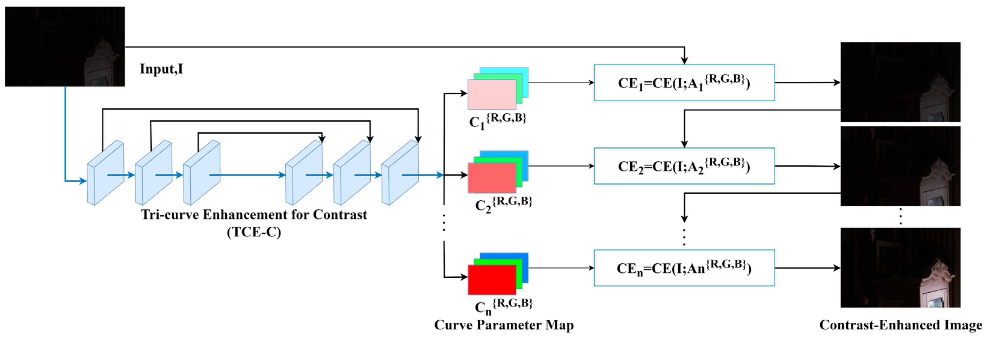
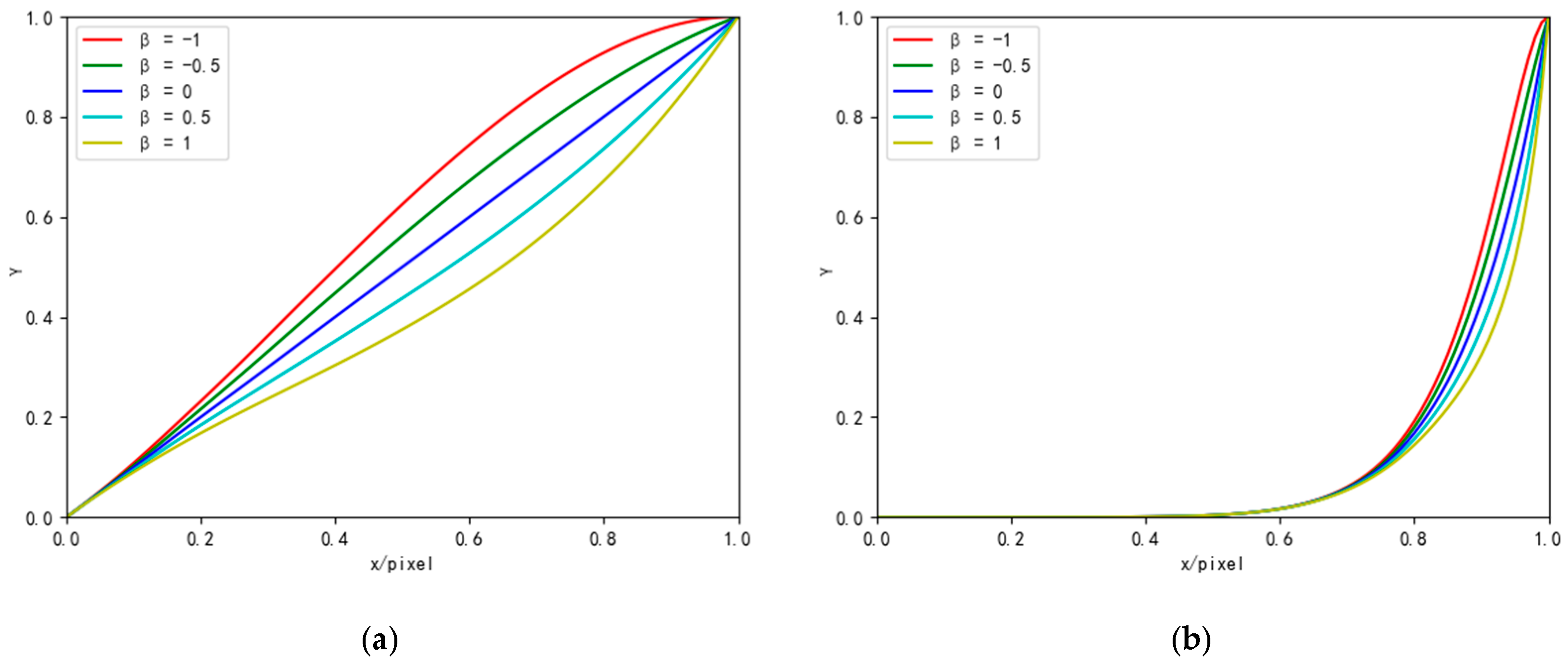
To address the challenges, we introduce the zero-reference triple-curve enhancement algorithm (Zero-TCE), a novel approach specifically designed to enhance low-light images. It possesses the capability to handle a diverse array of lighting conditions, encompassing backlight scenarios, uneven illumination, and insufficient lighting. By framing the task of low-light image enhancement as a unique curve estimation problem tailored to each individual image, Zero-TCE accepts a low-light image as an input and produces three high-order curves as the output, thereby facilitating significant improvements in image quality. These curves are then utilized to adjust the dynamic range of the input image at the pixel level to obtain an enhanced image. These three curves are meticulously designed to boost image brightness while avoiding overexposure, preserving the highlight regions of the original image, and enhancing image contrast without excessive enhancement, making the image appear more realistic. More importantly, the proposed network is lightweight, enabling more robust and precise dynamic range adjustment.

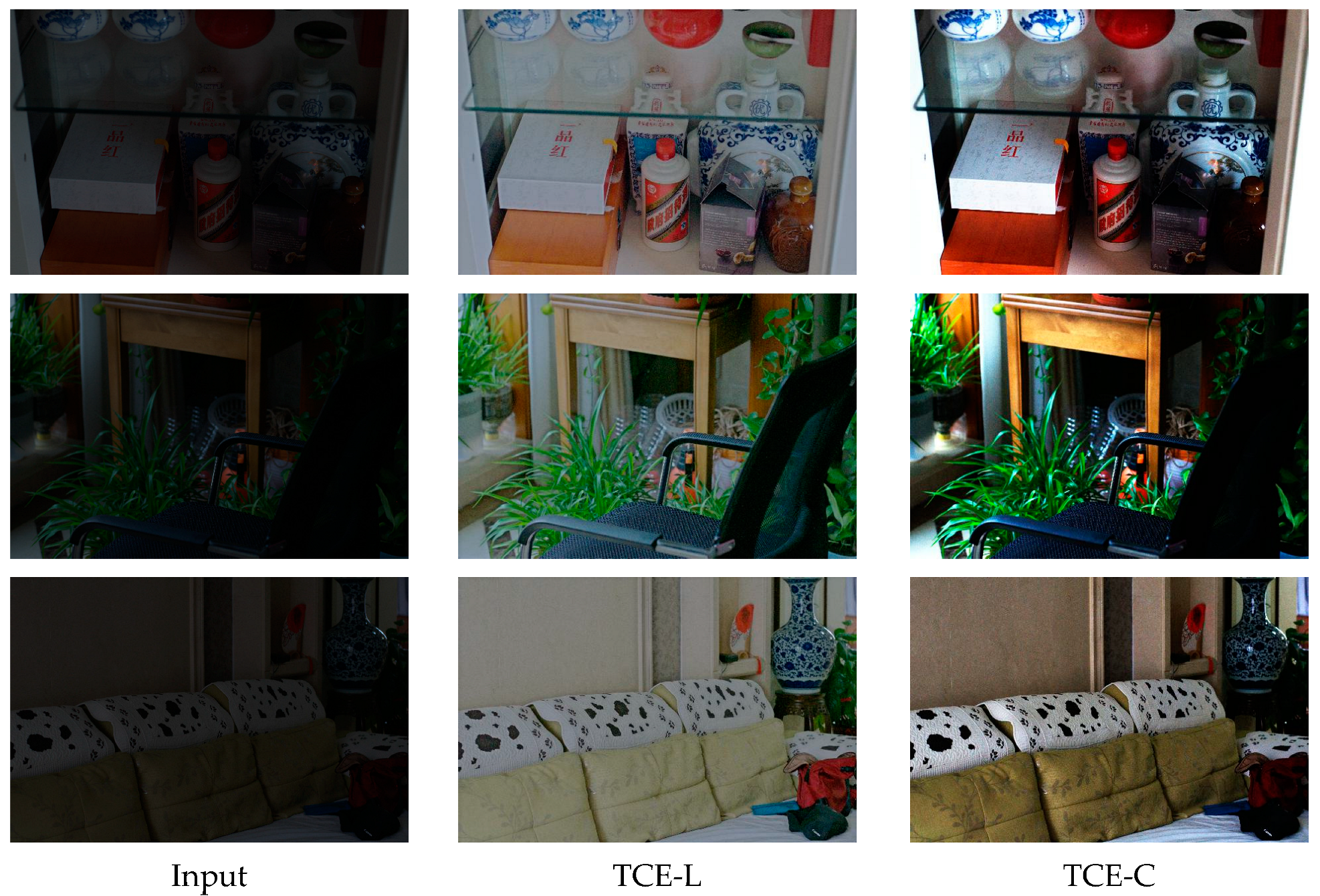
Firstly, we design two modules based on DCE-Net, the TCE-L and TCE-C modules, which output two curves that are specifically for enhancing image brightness and contrast, respectively. Additionally, we develop a multi-scale feature fusion (MFF) module that integrates multi-scale features from both the original and preliminarily enhanced images, taking into account the brightness distribution characteristics of low-light images, to obtain the optimal enhanced image. The key advantage of the proposed algorithm lies in its zero-reference nature, meaning no paired or unpaired data are required during training. This is achieved by adopting a set of non-reference loss functions, including spatial consistency loss, exposure control loss, color constancy loss, and illumination smoothness loss, to ensure image quality and avoid issues such as artifacts and color distortion. Furthermore, we incorporate the structural similarity index measure loss to preserve accurate image textures. These loss functions are designed to capture high-level features of images, rather than just pixel-level differences, thereby helping to improve the model’s ability to adapt to new lighting conditions. The contributions of this study are as follows:

• We propose Zero-TCE, a zero-reference dual-path network for low-light image enhancement based on multi-scale deep curve estimation. This network is independent of paired and unpaired training data, thereby mitigating the risk of overfitting.
• We design three image-specific curves that collectively enable brightness enhancement, contrast improvement, and multi-scale feature fusion for low-light images.
• We indirectly assess enhancement quality through task-specific non-reference loss functions, which preserve accurate image textures, enhance dark details, and avoid issues such as artifacts and color distortions.

The structure of the remainder of this paper is outlined as follows: Section 2 delves into related work, providing an overview of the current approach in the field. Section 3 presents a comprehensive description of the proposed Zero-TCE method, elucidating its intricacies in detail. In Section 4, we present and discuss the experimental results obtained through the application of Zero-TCE. Lastly, Section 5 concludes the paper by summarizing our findings and outlining potential directions for future research.

2. Related Work

Low-light image enhancement can be accomplished by adjusting curves in photo editing software, with the adaptive curve parameters being entirely contingent upon the input image. However, for particularly challenging low-light images, the optimal curve often exhibits a high degree of complexity. Drawing inspiration from curve toning techniques employed in photo editing software, the authors of algorithm [40] introduced Zero-DCE, an innovative approach that approximates the optimal high-degree curve by iteratively computing lower-degree curves. In this work, a second-degree brightness enhancement curve is applied in each step to enhance low-light images. The formula can be expressed as follows:

$$LE\left[I\left(\mathit{x}\right);A\left(\mathit{x}\right)\right]=I\left(\mathit{x}\right)+A\left(\mathit{x}\right)I\left(\mathit{x}\right)\left[1-I\left(\mathit{x}\right)\right],$$

(1)

where $I$ represents the input low-light image, $\mathit{x}$ denotes the pixel coordinates, the function $LE\left[I\left(\mathit{x}\right);A\left(\mathit{x}\right)\right]$ stands for the enhanced image output at $x$, and $A\left(\mathit{x}\right)$ represents the learned feature parameters, which have the same dimensions as the image. This algorithm progressively approximates higher-degree brightness enhancement curves by applying brightness enhancement multiple times. In step $t$ $\left(t\ge 1\right)$, the obtained enhanced output is as follows:

$$L{E}_t\left(\mathit{x}\right)=L{E}_{t-1}\left(\mathit{x}\right)+A_t\left(\mathit{x}\right)L{E}_{t-1}\left(\mathit{x}\right)\left[1-L{E}_{t-1}\left(\mathit{x}\right)\right].$$

(2)

Consequently, the challenge of low-light image enhancement is recast as the pursuit of acquiring the appropriate feature parameters. Specifically, this entails the discovery of the optimal pixel parameter mapping $A_t\left(\mathit{x}\right)$ at each step.

3. Materials and Methods

Based on the inherent mapping relationship between low-light image enhancement and deep curve estimation, we propose a zero-reference tri-curve image enhancement (Zero-TCE) network grounded in deep curve estimation. This network primarily comprises a tri-curve enhancement for light (TCE-L) module, a tri-curve enhancement for contrast (TCE-C) module, and a multi-scale feature fusion module (MFF). In this model, low-light images are first processed through two parameter estimation modules to generate corresponding parameter maps. These parameter maps are then input into the enhancement modules, where they undergo mapping and iterative calculations across the RGB channels of all input image pixels to obtain brightness-enhanced and contrast-enhanced images. Finally, in the HSV color space, leveraging the brightness distribution characteristics of the image, the preliminary enhanced images are fused with the original image through multi-scale feature fusion, yielding the final enhanced image. The overall network framework is illustrated in Figure 1.

3.1. Tri-Curve Enhancement for Light (TCE-L)

Images captured under low-light or backlight conditions often suffer from insufficient brightness and a lack of detail in dark areas due to inadequate lighting. To address this, we propose the use of TCE-L to adjust the brightness information about the images. The TCE-L framework is illustrated in Figure 2.

The input of TCE-L is a low-light image, and its output is a set of pixelated curve parameter maps corresponding to high-order curves. We employ a 7-layer convolutional neural network (CNN) [42] architecture. Each layer consists of 32 convolution kernels with a size of 3 × 3 and a stride of 1, followed by an ReLU activation function. The final layer uses a Tanh function to map the parameter maps into the range of −1 to 1, and a Split function is utilized to decompose the parameter map into 8 parameter maps with 3 channels each, which are then utilized by the enhancement module.

To enable automatic mapping of low-light images to their brightness-enhanced versions, we adopt a second-order light enhancement curve (LE-curve). The formula can be expressed as follows:

$$LE\left(I\left(\mathit{x}\right);\alpha \right)=I\left(\mathit{x}\right)+\alpha I\left(\mathit{x}\right)\left[1-I\left(\mathit{x}\right)\right],$$

(3)

where $I$ denotes the input low-light image, $\mathit{x}$ represents the pixel coordinates, and the function $LE\left(I\left(\mathit{x}\right);\alpha \right)$ signifies the enhanced image output at $x$. $\alpha \in \left[-1,1\right]$ is a trainable curve parameter that adjusts the magnitude of the LE curve and controls the exposure level concurrently. Each pixel is normalized to the range $\left[0,1\right]$, and all operations are performed on a per-pixel basis. To achieve more versatile adjustments and tackle challenging low-light environments, we iteratively apply the LE curve defined in Equation (3). Specifically, it can be expressed as follows:

$$L{E}_n\left(\mathit{x}\right)=L{E}_{n-1}\left(\mathit{x}\right)+{\alpha }_{n}L{E}_{n-1}\left(\mathit{x}\right)\left[1-L{E}_{n-1}\left(\mathit{x}\right)\right],$$

(4)

where $n$ is the number of iterations, controlling the curvature of the curve. In this paper, we set $n$ to 8, which suffices for most scenarios. When $n$ equals 1, Equation (4) is reduced to Equation (3). Figure 3 displays the LE curves with different parameters. From this figure, it can be observed that each pixel value of the enhanced image falls within a certain range, and the curve is monotonic and differentiable during gradient backpropagation. As seen in Figure 3b, after iterations, the curve gains stronger adjustment capabilities, enabling it to more effectively enhance image brightness. Global mapping often results in the over- or under-processing of local regions, leading to the amplification of noise along with the enhancement of dark detail. To address this, we define $\alpha$ as a pixel-wise parameter, meaning each pixel of the input image is assigned an optimal fitting curve in order to adjust its dynamic range. This approach avoids drastic adjustments to image pixels directly, as shown in Equation (2).

3.2. Tri-Curve Enhancement for Contrast (TCE-C)

Analogous to the TCE-L module, we introduce the TCE-C module, which is designed to augment the contrast of low-light images, thereby enhancing the finer details within darker regions. The framework of TCE-C is illustrated in Figure 4.

We observe that, while TCE-L is generally effective in brightening images and preserving details, it does not significantly enhance contrast, and its effectiveness may be unsatisfactory under extreme low-light conditions. Therefore, we propose a third-order contrast-enhancement curve (CE curve), which can be expressed as follows:

$$CE\left(I\left(\mathit{x}\right);\beta \right)=I\left(\mathit{x}\right)-\beta I{\left(\mathit{x}\right)}^2\left[1-I\left(\mathit{x}\right)\right].$$

(5)

The formula for high-order curves can be expressed as follows:

$$C{E}_n\left(\mathit{x}\right)=C{E}_{n-1}\left(\mathit{x}\right)-{\beta }_n{\left[C{E}_{n-1}\left(\mathit{x}\right)\right]}^2\left[1-C{E}_{n-1}\left(\mathit{x}\right)\right].$$

(6)

It is evident that this curve meets the requirements of the network. Moreover, by increasing the order of the curve compared to the original, the enhancement effect becomes more pronounced. Figure 5a displays CE curves with different parameters. Compared to Figure 3a, the CE curve exhibits stronger adjustment capabilities.

Similarly, to address more complex low-light environments, we introduce a high-order adjustment mechanism for the CE curve by defining $\beta$ as a pixel-wise parameter:

$$C{E}_n\left(\mathit{x}\right)=C{E}_{n-1}\left(\mathit{x}\right)-C_n{\left[C{E}_{n-1}\left(\mathit{x}\right)\right]}^2\left[1-C{E}_{n-1}\left(\mathit{x}\right)\right].$$

(7)

We also set $n$ to 8. When $n$ equals 1, Equation (6) is reduced to Equation (5). Figure 5b displays various high-order curves. Compared to the curves in Figure 5a and Figure 3b, they offer superior adjustment capabilities for enhancement effects. The enhancement effects of the TCE-L and TCE-C modules are shown in Figure 6. It is evident that TCE-L effectively increases the brightness of low-light images, while TCE-C significantly enhances their contrast.

3.3. Multi-Scale Feature Fusion (MFF)

The TCE-L module can effectively increase the brightness of images, but the contrast remains low. The TCE-C module can significantly enhance the image contrast, yet its brightening effect is limited, and it tends to cause overexposure due to excessive contrast enhancement in brighter areas. Therefore, to fully leverage the advantages of these two modules, we propose an adaptive image fusion algorithm, which can be expressed as follows:

$$MF\left(\mathit{x},{\mathit{x}}_L,{\mathit{x}}_C\right)=k\mathit{x}+\left(1-k\right)\left[\gamma {\mathit{x}}_L+\left(1-\gamma \right){\mathit{x}}_C\right],$$

(8)

where $\mathit{x}$ represents the pixel matrix of the original low-light image, ${\mathit{x}}_L$ represents the pixel matrix of the image enhanced by the TCE-L module, and ${\mathit{x}}_C$ denotes the pixel matrix of the image enhanced by the TCE-C module. $k$ and $\gamma$ are adaptive weights used to adjust the balance between the original image and the enhanced images, as well as between the two enhanced images, respectively, with values ranging from 0 to 1. Figure 5 demonstrates the processing effects of the TCE-L module, TCE-C module, and MFF module individually, as well as the effect without the MFF module. As observed in Figure 7, when pixel values are too high (i.e., brighter) or too low (i.e., darker), TCE-L performs better in enhancing the dark details of the image. Thus, $\gamma$ should be larger. When pixel values fall between these two extremes, TCE-C significantly enhances image contrast and highlights certain details, resulting in better enhancement. Hence, $\gamma$ should be smaller. Based on these findings, we designe a quadratic curve, according to the brightness characteristics of the input image, for the adaptive fusion of the two enhanced images. The formula can be expressed as follows:

$$\gamma ={\displaystyle \frac{1}{{128}^2}}{\left[{\max }_{C\left\{r,g,b\right\}}\left\{I^C\left(\mathit{x}\right)\right\}-128\right]}^2,$$

(9)

where ${\max }_{C\left\{r,g,b\right\}}\left\{I^C\left(\mathit{x}\right)\right\}$ represents the maximum value among the three color channels for a given input $I\left(\mathit{x}\right)$ (i.e., the brightness of the original image at location $x$).

When enhancing low-light images, the high-light areas, particularly sky regions, often suffer from overexposure and detail loss due to excessive enhancement. Moreover, the RGB color space, consisting of the primary colors red, green, and blue, is widely used in digital imaging because of its intuitiveness and compatibility with hardware. However, the RGB color space lacks precision in handling color distortion, especially when precise control over color variations is required. Both the TCE-L and TCE-C modules directly process the R (red), G (green), and B (blue) channels, which can easily lead to color distortion. The HSV color space offers an alternative perspective for understanding and manipulating color. It decomposes color into three components—hue, saturation, and value—enabling more intuitive and precise adjustments to color. Therefore, our approach processes the image in the HSV color space and designs a weight curve based on the grayscale variation information in the enhanced image for adaptive fusion between the original and enhanced images. First, we determine the brightness value $g_m$ for each pixel within the input image by employing a weighted average approach to the R, G, and B color components. This method assigns varying degrees of importance to each component, which can be mathematically formulated as follows:

$$g_m=0.11R\left(x\right)+0.59G\left(x\right)+0.30B\left(x\right).$$

(10)

Then, a weight coefficient $k$ is introduced, which can be adaptively adjusted according to the brightness distribution characteristics of the input image. The formula can be expressed as follows:

$$k=-{\displaystyle \frac{1}{255}}\left(g_m-2\right)g_m.$$

(11)

In summary, the MFF module adaptively fuses the brightness values (V) of the original image, the brightness-enhanced image, and the contrast-enhanced image, and then combines them with the hue (H) and saturation (S) of the original image to produce the final enhanced image. The enhancement effects of each module are shown in Figure 7. The algorithm in this paper not only significantly enhances the dark details of the image but also successfully preserves the edge details in the high-brightness regions of the original image, effectively avoiding overexposure and color distortion. Furthermore, it mitigates the noise amplification that typically accompanies the brightening of dark details and contrast enhancement. This underscores the superiority and practical viability of the proposed algorithm in processing low-light images.

3.4. Non-Reference Loss Functions

To facilitate zero-reference learning, we employ a suite of differentiable, non-reference losses to assess the quality of the enhanced images. Specifically, we leverage five distinct types of losses to train the Zero-TCE model.

3.4.1. Spatial Consistency Loss

The spatial consistency loss $L_{spa}$ encourages spatial coherence in the enhanced image by maintaining the differences observed between adjacent regions in the input image and its enhanced counterpart. This can be mathematically formulated as follows:

$$L_{spa}={\displaystyle \frac{1}{K}}{\displaystyle \sum _{i=1}^K{\displaystyle \sum _{j\in \Omega \left(i\right)}{\left[\left|Y_i-Y_j\right|-\left|I_i-I_j\right|\right]}^2}},$$

(12)

where $K$ is the number of local regions, $\Omega \left(i\right)$ represents the four adjacent regions (top, bottom, left, right) centered around region $i$, and $Y$ and $I$ denote the average intensity values of the enhanced image and the original image, respectively. Empirically, the size of the local region is set to 4 × 4.

3.4.2. Exposure Control Loss

To mitigate the presence of underexposed or overexposed areas, we regulate the exposure level by utilizing exposure control loss. This loss metric quantifies the deviation between the average intensity value of local regions and a predefined, optimal exposure level. Following established methodologies [43,44], we set $E$ to 0.6. The loss function $L_{e\mathit{x}p}$ can be mathematically formulated as follows:

$$L_{e\mathit{x}p}={\displaystyle \frac{1}{M}}{\displaystyle \sum _{K=1}^M\left|Y_K-E\right|},$$

(13)

where $M$ denotes the total count of non-overlapping local patches, and $Y$ signifies the mean intensity value of these patches within the enhanced image.

3.4.3. Color Constancy Loss

Drawing inspiration from the Gray World Color Constancy Hypothesis [45], we introduce a color constancy loss to counteract potential color distortions in the enhanced images. This not only corrects biases but also fosters correlations among the three adjustment channels, thereby ensuring color accuracy. The mathematical formulation of $L_{col}$ is as follows:

$$L_{col}={\displaystyle \sum _{\forall \left(p,q\right)\in \epsilon }{\left(J^p-J^q\right)}^2},\epsilon =\left\{\left(R,G\right),\left(R,B\right),\left(G,B\right)\right\},$$

(14)

where $J^p$ represents the average intensity value of channel $p$ in the enhanced image, and $\left(p,q\right)$ denotes a pair of channels.

3.4.4. Illumination Smoothness Loss

To maintain the monotonic relationship between adjacent pixels, we adopt an illumination smoothness loss $L_{t{v}_A}$, which can be expressed as follows:

$$L_{t{v}_A}={\displaystyle \frac{1}{N}}{\displaystyle \sum _{n=1}^N{\displaystyle \sum _{C\in \left\{R,G,B\right\}}{\left(\left|{\nabla }_x{A}_n^c\right|+\left|{\nabla }_y{A}_n^c\right|\right)}^2}},$$

(15)

where $N$ represents the number of iterations, and ${\nabla }_x$ and ${\nabla }_y$ denote the horizontal and vertical gradient operations, respectively.

3.4.5. Structure Similarity Index Measure Loss

To avoid image distortion, we employ the structural similarity index measure (SSIM) loss $L_{ssim}$. SSIM [46] is a perception-based model used to evaluate the similarity between two images. It assesses image similarity or detects degrees of distortion by considering three aspects: luminance, structure, and contrast. It can be mathematically formulated as follows:

$$SSIM={\displaystyle \frac{1}{M\times N}}{\displaystyle \sum _{i=1}^M{\displaystyle \sum _{j=2}^N\frac{\left(2{\mu }_X{\mu }_Y+C_1\right)\left(2{\sigma }_{XY}+C_2\right)}{\left({{\mu }_X}^2+{{\mu }_Y}^2+C_1\right)\left({{\sigma }_X}^2+{{\sigma }_Y}^2+C_2\right)}}},$$

(16)

where $M$ and $N$ represent the height and width of the images, respectively; $X$ and $Y$ denote the two images being compared; ${\mu }_X$ and ${\mu }_Y$ are the mean values of images $X$ and $Y$; ${\sigma }_X$ and ${\sigma }_Y$ are the variances in images $X$ and $Y$; ${\sigma }_{XY}$ is the covariance between images $X$ and $Y$; and $C_1$ and $C_2$ are constants, which are typically set to $C_1={\left(K_1\cdot Q\right)}^2$ and $C_2={\left(K_2\cdot Q\right)}^2$, with $K_1=0.01$, $K_2=0.03$, and $Q=255$, for stability.

We incorporate the SSIM error to regulate the level of distortion in the enhanced images. Given that a higher SSIM value signifies superior image enhancement quality, the formula for calculating this error can be expressed as follows:

$$L_{ssim}=1-SSIM,$$

(17)

3.4.6. Total Loss

The total error can be mathematically formulated as follows:

$$L_{total}=W_{total}\left(L_{spa}+L_{e\mathit{x}p}+W_{col}{L}_{col}+W_{t{v}_A}{L}_{t{v}_A}\right)+\left(1-W_{total}\right)L_{ssim},$$

(18)

where $W_{total}$, $W_{col}$, and $W_{t{v}_A}$ represent the weights assigned to the respective loss components. Specifically, these three weight parameters are, respectively, responsible for regulating the overall loss, the color constancy loss, and the illumination smoothness loss. Their values are fine-tuned through numerous experiments, based on the significance of each loss function’s contribution to the ultimate image quality, in order to achieve a harmonious balance among the impacts of various loss functions.

4. Experiments and Results

In this section, we will delve deeply into the implementation specifics of our approach to enhance low-light images. Following this, we will undertake both qualitative and quantitative comparisons with cutting-edge techniques for low-light image enhancement, utilizing conventional evaluation metrics, such as Peak Signal-to-Noise Ratio (PSNR) [47], structural similarity index measure (SSIM) [46], Perceptual Image Quality Evaluator (PIQE) [48], and Blind/Referenceless Image Spatial Quality Evaluator (BRISQUE) [49]. Additionally, we perform ablation experiments to demonstrate the effectiveness of each component in our proposed method.

4.1. Implementation Details

The framework is implemented using PyTorch and runs on an NVIDIA 4090 GPU equipped with 24 GB of memory. During training, we employ a batch size of 8. The initialization of the weights for each layer follows a standard Gaussian distribution with a mean of zero and a standard deviation of 0.02, while the biases are set to a constant value. To achieve better network optimization, we employ the Adam optimizer. To balance the impact of various loss functions on image quality, after referencing the Zero-DCE algorithm and conducting experimental validation, we set the values of $W_{col}$ and $W_{t{v}_A}$ to 0.5 and 20, respectively. Furthermore, addressing the potential for significant distortion in images processed by the Zero-DCE algorithm, we introduce the SSIM loss and prioritize it as a core component, making its effect comparable to the combined action of other loss functions. Consequently, we assign a value of 0.5 to $W_{total}$ to ensure the comprehensive enhancement of image quality.

To fully harness the potential of wide-dynamic-range adjustment during the training process, we incorporate a diverse set of low-light and overexposed images from the SICE dataset [50] into the training set, comprising a total of 2002 images. This approach ensures that our model is exposed to a wide range of lighting conditions, enhancing its ability to generalize and adapt to various scenarios. Furthermore, to avoid inconsistencies in image size when the network processes them, all training images are resized to 512 × 512 pixels, which not only accelerates the network’s inference speed but also enhances its accuracy.

4.2. Qualititative Evaluation

In this section, we conduct a comprehensive comparison of our method against several state-of-the-art approaches for low-light image enhancement. Our benchmark includes two conventional methods (MSRCR [19], Dong [25]), three supervised methods (KinD++ [33], RetinexNet [31], Retinexformer [32]) and five unsupervised methods (EnlightGAN [36], Zero-DCE++ [41], CLIP-LIT [37], NeRCo [38], Colie [39]).

Figure 8 displays the training/testing curves that illustrate the variation in total loss over epochs. These curves mirror the training process of the model across four distinct datasets: SICE, LOLv1 [31], LOLv2-real, and LOLv2-synthetic [51]. It is observable from the figure that, when working on the SICE and LOLv1 datasets, the model converges after approximately 50 training epochs, exhibiting stable training and testing losses. On the LOLv2-real dataset, the model converges more rapidly, achieving convergence after around 25 epochs. Meanwhile, on the LOLv2-synthetic dataset, despite the slower convergence rate, the testing loss gradually decreases during the training process and subsequently stabilizes alongside the training loss, demonstrating strong generalization abilities. In summary, these curves indicate that the model is capable of effective training on different datasets and can swiftly identify optimal or near-optimal solutions.

Figure 9, Figure 10, Figure 11, Figure 12, Figure 13, Figure 14 and Figure 15 show some representative results for visual comparison, drawing from the LOLv1 dataset (500 images), the LOLv2-real dataset (789 images), the LOLv2-synthetic dataset (1000 images), the DICM dataset [52] (42 images), the MEF dataset [53] (16 images), and the NPE dataset [54] (8 images). The LOL dataset captures pairs of low-light and normal-light images by adjusting the camera’s exposure time and ISO settings, thereby offering a comprehensive resource for research on image enhancement in low-light conditions. It has v1 and v2 versions. LOL-v2 is divided into real and synthetic subsets. To further validate the robustness of the proposed algorithm, we augment our testing to include extreme scenarios, encompassing overexposure and complexly fluctuating lighting conditions among other challenging settings. We choose to conduct experiments on the ExDark dataset [55], which comprises 7363 images captured under varying degrees of illumination, ranging from extreme darkness to dusk. These images exhibit exceptionally complex lighting conditions, encompassing 10 distinct lighting scenarios, and simulate a wide range of real-world low-light environments, such as night vision and scenes illuminated by faint moonlight.

For traditional algorithms, the MSRCR algorithm [19] significantly enhances image contrast but limits brightening effects, with dark regions remaining dim and even accompanied by color distortion. The Dong algorithm [25] improves image brightness and enhances edge details, but some edges are over-enhanced, making the image unnatural and introducing noticeable block effects that compromise the overall image quality. Among supervised deep learning algorithms, the KinD++ algorithm [33] effectively boosts image brightness and contrast, but introduces excessive noise in dark regions after enhancement, resulting in the loss of edge details. The RetinexNet algorithm [31] produces significant noise and color distortion issues. The Retinexformer algorithm [32] causes obvious overexposure and color distortion in the high-light areas of the image. Among unsupervised deep learning algorithms, the EnlightGAN algorithm [36] enhances the brightness of dark regions while strengthening edge details, but color distortion and over-enhancement in bright regions lead to the loss of some edge details, with insufficiently natural transitions between light and dark areas causing noticeable color differences. The Zero-DCE++ algorithm [41] effectively improves image brightness but suffers from severe color distortion. The CLIP-LIT algorithm [37] demonstrates a remarkable ability to augment the fine details within the dark regions of low-light images and significantly enhances their contrast. However, in extreme scenarios, it tends to over-brighten these areas, which can result in partial color distortion and a noticeable degradation of edge details, which is particularly evident in skyscapes. The NeRCo algorithm [38] effectively amplifies image brightness, but at the expense of introducing pronounced color distortions and a considerable loss of edge integrity. The Colie algorithm [39] performs well but loses edge details in high-light areas. In contrast, the algorithm proposed in this paper not only effectively enhances image brightness and contrast but also preserves edge details in high-light areas, avoids overexposure, and overall meets the requirements of both human and computer vision more closely.

4.3. Quantitative Evaluation

Since SSIM has already been described, here, we briefly describe the PSNR evaluator as follows. PSNR (Peak Signal-to-Noise Ratio) is one of the most prevalent and widely adopted objective evaluation metrics for image quality assessment. A higher PSNR value signifies a lower level of noise interference and distortion within the image, reflecting improved fidelity and clarity. This metric can be mathematically formulated as follows:

$$PSNR=10\cdot \lg {\displaystyle \frac{{\displaystyle \sum _{i=1}^M{\displaystyle \sum _{j=1}^N{\left\{\max \left[f\left(i,j\right)\right]\right\}}^2}}}{{\displaystyle \sum _{i=1}^M{\displaystyle \sum _{j=1}^N{\left[f^{\prime }\left(i,j\right)-f(i,j)\right]}^2}}}},$$

(19)

where $M$ represents the height of the image, $N$ represents the width of the image, $\max \left[f\left(i,j\right)\right]$ represents the maximum pixel value of the image, and $f\left(i,j\right)$ denotes the pixel value at the row $i$ and column $j$ of the image. PIQE is a no-reference image quality assessment metric that leverages perceptual features to evaluate image quality by mimicking the perception mechanisms of the human visual system. It specifically calculates the image quality score by analyzing the block structure and noise characteristics of the image. A lower PIQE score indicates superior image quality. BRISQUE is a no-reference image quality evaluation metric that relies on natural scene statistics. By extracting histogram data, local features, contrast, texture, and edge information from the image, it accurately and stably identifies distortion effects that affect human visual perception. A lower BRISQUE score signifies a more natural appearance of the image, thereby indicating higher image quality.

The final experimental results, presented in

Table 1. Quantitative comparison results of (LOLv1, LOLv2-real, LOLv2-synthetic, DICM, MEF, NPE, and ExDark) datasets using the PSNR metric. A higher value of the PSNR metric indicates a better performance. The first, second, and third best scores are highlighted with red, blue, and green colors, respectively.

Learning	Datasets	LOLv1	LOLv2-Real	LOLv2-Synthetic	DICM	MEF	NPE	ExDark	Avg
Conventional	MSRCR	6.239	6.253	13.077	12.443	12.056	15.938	10.016	10.860
	Dong	10.425	12.474	12.258	13.526	12.315	12.577	12.449	12.285
Supervised	KinD++	7.841	8.541	12.906	13.328	11.763	12.827	12.501	11.387
	RetinexNet	8.438	9.898	11.011	11.658	10.227	11.317	10.429	10.425
	Retinexformer	7.798	9.225	11.878	10.449	10.400	12.520	11.462	10.533
Unsupervised	EnlightGAN	10.275	10.377	12.356	12.772	11.578	13.491	11.467	11.759
	Zero-DCE++	13.049	13.602	13.667	14.640	13.801	13.870	13.370	13.714
	CLIP-LIT	15.634	14.846	15.859	16.272	15.633	15.954	15.290	15.641
	NeRCo	8.078	9.393	14.590	14.341	12.253	18.876	12.838	12.910
	Colie	10.423	10.599	13.524	14.857	13.750	13.823	14.280	13.037
	Ours	15.213	16.084	18.100	18.992	17.653	17.801	17.019	17.266

,

Table 2. Quantitative comparison results of (LOLv1, LOLv2-real, LOLv2-synthetic, DICM, MEF, NPE, and ExDark) datasets using the SSIM metric. A higher value of the SSIM metric indicates better performance. The first, second, and third best scores are highlighted with red, blue, and green colors, respectively.

Learning	Datasets	LOLv1	LOLv2-Real	LOLv2-Synthetic	DICM	MEF	NPE	ExDark	Avg
Conventional	MSRCR	0.153	0.119	0.455	0.466	0.361	0.527	0.342	0.346
	Dong	0.160	0.214	0.490	0.489	0.359	0.573	0.425	0.387
Supervised	KinD++	0.156	0.191	0.505	0.501	0.339	0.547	0.401	0.377
	RetinexNet	0.117	0.166	0.455	0.436	0.323	0.586	0.332	0.345
	Retinexformer	0.177	0.170	0.503	0.392	0.334	0.555	0.388	0.360
Unsupervised	EnlightGAN	0.180	0.190	0.517	0.485	0.360	0.649	0.377	0.394
	Zero-DCE++	0.264	0.275	0.545	0.528	0.429	0.634	0.442	0.445
	CLIP-LIT	0.307	0.293	0.585	0.532	0.458	0.683	0.497	0.479
	NeRCo	0.162	0.155	0.541	0.488	0.371	0.738	0.386	0.406
	Colie	0.176	0.161	0.524	0.506	0.410	0.618	0.477	0.410
	Ours	0.306	0.334	0.670	0.706	0.566	0.721	0.598	0.557

,

Table 3. Quantitative comparison results of (LOLv1, LOLv2-real, LOLv2-synthetic, DICM, MEF, NPE, and ExDark) datasets using the PIQE metric. A lower value of the PIQE metric indicates better performance. The first, second, and third best scores are highlighted with red, blue, and green colors, respectively.

Learning	Datasets	LOLv1	LOLv2-Real	LOLv2-Synthetic	DICM	MEF	NPE	ExDark	Avg
Conventional	MSRCR	19.405	29.207	20.043	16.015	19.812	24.268	18.547	21.042
	Dong	15.136	25.908	8.807	8.657	7.960	11.529	12.426	12.918
Supervised	KinD++	18.626	18.182	16.501	11.911	18.099	13.090	20.745	16.736
	RetinexNet	22.129	32.463	12.252	12.965	18.099	10.926	13.314	17.450
	Retinexformer	11.338	6.802	9.214	5.153	12.159	7.164	12.655	9.212
Unsupervised	EnlightGAN	9.729	20.586	9.611	6.031	8.688	12.653	13.993	11.613
	Zero-DCE++	7.926	23.957	11.247	6.784	8.172	12.640	15.325	12.293
	CLIP-LIT	13.343	26.386	11.024	9.565	8.714	11.614	13.146	13.399
	NeRCo	10.436	9.303	9.593	22.084	15.479	21.965	25.287	16.307
	Colie	10.933	25.036	11.317	7.962	12.753	13.702	15.599	13.900
	Ours	9.230	21.418	9.023	6.287	6.532	11.057	12.340	10.841

,

Table 4. Quantitative comparison results of (LOLv1, LOLv2-real, LOLv2-synthetic, DICM, MEF, NPE, and ExDark) datasets using the BRISQUE metric. A lower value of the BRISQUE metric indicates better performance. The first, second, and third best scores are highlighted with red, blue, and green colors, respectively.

Learning	Datasets	LOLv1	LOLv2-Real	LOLv2-Synthetic	DICM	MEF	NPE	ExDark	Avg
Conventional	MSRCR	0.496	0.499	0.493	0.492	0.492	0.492	0.492	0.494
	Dong	0.497	0.489	0.511	0.540	0.488	0.631	0.504	0.523
Supervised	KinD++	0.503	0.498	0.501	0.487	0.539	0.456	0.501	0.498
	RetinexNet	0.504	0.500	0.492	0.496	0.510	0.566	0.500	0.510
	Retinexformer	0.505	0.494	0.506	0.515	0.519	0.531	0.510	0.511
Unsupervised	EnlightGAN	0.499	0.499	0.517	0.526	0.537	0.494	0.513	0.512
	Zero-DCE++	0.495	0.493	0.509	0.546	0.539	0.487	0.504	0.511
	CLIP-LIT	0.491	0.495	0.508	0.529	0.499	0.601	0.504	0.518
	NeRCo	0.512	0.502	0.515	0.525	0.549	0.533	0.505	0.520
	Colie	0.518	0.511	0.519	0.508	0.453	0.490	0.508	0.501
	Ours	0.493	0.492	0.491	0.477	0.509	0.436	0.497	0.485

and

Table 5. Runtime comparison (in second) results of (LOLv1, LOLv2-real, LOLv2-synthetic, DICM, MEF, NPE, and ExDark) datasets. The first, second, and third best scores are highlighted with red, blue, and green colors, respectively.

Learning	Datasets	LOLv1	LOLv2-Real	LOLv2-Synthetic	DICM	MEF	NPE	ExDark	Avg
Conventional	MSRCR	0.400	0.439	0.378	0.480	0.254	0.333	0.797	0.440
	Dong	0.508	0.537	0.340	0.692	0.349	0.493	1.539	0.637
Supervised	KinD++	5.042	6.278	4.294	6.617	2.977	4.225	4.093	4.789
	RetinexNet	1.209	1.219	0.804	0.961	0.934	0.685	3.538	1.336
	Retinexformer	0.806	0.510	0.467	0.750	0.688	1.054	2.124	0.914
Unsupervised	EnlightGAN	0.990	0.295	0.165	0.284	0.178	0.219	0.535	0.381
	Zero-DCE++	0.061	0.204	0.126	0.069	0.170	0.262	0.084	0.140
	CLIP-LIT	0.149	0.236	0.577	0.269	0.453	0.866	0.279	0.404
	NeRCo	0.386	0.410	0.271	0.484	0.669	0.888	0.262	0.482
	Colie	0.759	0.760	0.820	1.190	1.313	1.625	1.637	1.158
	Ours	0.346	0.390	0.324	0.418	0.381	0.324	0.825	0.430

, demonstrate the superior performance of the proposed algorithm across all evaluated metrics. Although it slightly lags behind the Retinexformer algorithm in the PIQE metric, the Retinexformer significantly underperforms the proposed algorithm in other metrics, suggesting potential over-processing during enhancement, resulting in the loss of image details and a certain degree of distortion. In terms of processing speed, unsupervised deep learning algorithms generally exhibit faster performances, whereas the proposed algorithm is comparable to the CLIP-LIT algorithm, completing the processing of a single image within an average of 0.5 s. In contrast, the proposed algorithm demonstrates significant advantages across all metrics, with notably higher PSNR and SSIM values. This not only validates the effectiveness of our algorithm in enhancing image contrast and brightness but also highlights its ability to preserve low distortion levels while enhancing the dark details in low-light images, achieving a balance between computational efficiency and enhancement performance. These results fully underscore the efficiency and practicality of our algorithm in processing low-light images.

Based on the comprehensive results shown in Figure 9, Figure 10, Figure 11, Figure 12, Figure 13, Figure 14 and Figure 15 and Table 1, Table 2, Table 3, Table 4 and Table 5, the proposed algorithm performs excellently in both subjective and objective evaluations. It enhances the brightness and contrast of low-light images, highlights dark details, and effectively suppresses color distortion, resulting in images with better visibility.

4.4. Ablation Study

4.4.1. Contribution of Each Module

To thoroughly evaluate the individual contributions and overall synergistic effects of each module in the proposed algorithm, we conduct tests on the DICM, MEF, and NPE datasets. Qualitative and quantitative assessments are set up for scenarios where the TCE-L module acts alone, the TCE-C module acts alone, the MFF module is removed (without MFF module, -w/o MFF), the TCE-L module is removed (without TCE-L module, -w/o TCE-L), and the TCE-C module is removed (without TCE-C module, -w/o TCE-C).

Based on the results presented in Figure 16 and

Table 6. Quantitative comparison results of (DICM, MEF, and NPE) datasets using PSNR, SSIM, PIQE, and BRISQUE metrics. The best scores are highlighted in bold, where ↑ means bigger values are better, and ↓ means smaller values are better.

Methods			PSNR↑	SSIM↑	PIQE↓	BRISQUE↓
DCE-L	DCE-C	MFF
√			14.104	0.525	9.199	0.524
	√		10.196	0.581	13.441	0.492
√	√		13.198	0.544	9.540	0.532
	√	√	16.668	0.613	9.851	0.505
√		√	17.656	0.611	8.177	0.538
√	√	√	18.149	0.664	8.116	0.474

, the TCE-L module notably enhances the brightness of low-light images, but it sacrifices some edge details and amplifies noise to some extent, rendering the image’s detail hierarchy slightly blurred. Furthermore, the image experiences significant color distortion, resulting in lower PSNR and SSIM values. The TCE-C module effectively boosts the contrast of low-light images, but over-enhancement leads to severe overexposure, making the image appear unnatural and compromising its quality, giving higher BRISQUE and PIQE values. Processing without the MFF module, while being capable of combining the strengths of both the TCE-L and TCE-C modules, tends to overexpose the bright areas of the original image, particularly the sky region, causing detail loss and apparent distortion. Consequently, its PSNR and SSIM values are also lower. When all modules are integrated, the proposed method achieves a more balanced enhancement effect.

As shown in Table 6, after integrating all modules, the proposed method significantly achieves optimal values across all indicators. Therefore, both qualitative and quantitative evaluations demonstrate that all modules in the proposed method have a positive impact on the enhancement results.

4.4.2. Contribution of Each Loss

To thoroughly evaluate the roles of each loss function in the proposed algorithm, we conduct tests on the LOLv1, LOLv2-real, and LOLv2-synthetic datasets. Qualitative and quantitative assessments are set up for scenarios where the proposed algorithm excludes $L_{spa}$ (without $L_{spa}$, -w/o $L_{spa}$), $L_{e\mathit{x}p}$ (without $L_{e\mathit{x}p}$, -w/o $L_{e\mathit{x}p}$), $L_{col}$ (without $L_{col}$, -w/o $L_{col}$), $L_{t{v}_A}$ (without $L_{t{v}_A}$, -w/o $L_{t{v}_A}$), and $L_{ssim}$ (without $L_{ssim}$, -w/o $L_{ssim}$).

By comparing and analyzing the data presented in Figure 17 and

Table 7. Quantitative comparison results of (LOLv1, LOLv2-real, and LOLv2-synthetic) datasets using PSNR, SSIM, BRISQUE, and PIQE metrics. The best scores are highlighted in bold, where ↑ means bigger values are better, and ↓ means smaller values are better.

Methods					PSNR↑	SSIM↑	BRISQUE↓	PIQE↓
${\mathit{L}}_{\mathit{s}\mathit{p}\mathit{a}}$	${\mathit{L}}_{\mathit{e}\mathit{x}\mathit{p}}$	${\mathit{L}}_{\mathit{c}\mathit{o}\mathit{l}}$	${\mathit{L}}_{\mathit{t}{\mathit{v}}_{\mathit{A}}}$	${\mathit{L}}_{\mathit{s}\mathit{s}\mathit{i}\mathit{m}}$
	√	√	√	√	7.428	0.184	0.506	16.527
√		√	√	√	13.434	0.123	0.497	24.781
√	√		√	√	12.475	0.345	0.504	16.924
√	√	√		√	8.048	0.124	0.495	16.602
√	√	√	√		7.674	0.223	0.496	18.886
√	√	√	√	√	16.466	0.437	0.492	13.890

, we can clearly observe that removing $L_{spa}$ significantly reduces the contrast of the enhanced image, leading to severe image distortion. This change is directly reflected in the noticeable decline in PSNR and SSIM values, highlighting the indispensable role of $L_{spa}$ in maintaining the difference in adjacent areas between the input and enhanced images. Similarly, excluding $L_{e\mathit{x}p}$ makes it difficult to effectively restore low-light areas, thereby adversely affecting the overall image quality, as evidenced by a significant increase in the PIQE value. Furthermore, when $L_{col}$ is ignored, meaning the interrelationships among the three color channels are not adequately considered, this results in severe color distortion and an unnatural appearance of the image, leading to unsatisfactory PSNR and PIQE evaluations. Additionally, removing $L_{t{v}_A}$ disrupts the correlation between adjacent areas of the image, causing obvious artifact phenomena and similarly resulting in severe image distortion, with both PSNR and SSIM values dropping substantially. Lastly, excluding $L_{ssim}$ exacerbates image distortion, causing the significant loss of edge details and rendering the entire image unusually blurry, with both PSNR and SSIM values decreasing markedly. In contrast, when all loss functions are effectively integrated, the image enhancement effect reaches an optimal state. This not only demonstrates the unique contributions of each loss function in the image enhancement task but also emphasizes the importance of their mutual synergy and collective action in enhancing image quality.

As shown in Table 7, after integrating all loss functions, the proposed method significantly achieves optimal values across all indicators. Therefore, both qualitative and quantitative evaluations indicate that all loss functions in the proposed method have a positive impact on the enhancement results.

4.4.3. Contribution of Each Loss Weight

To validate the effectiveness of the proposed algorithm, we conduct tests on the DICM, MEF, and ExDark datasets. Drawing inspiration from the parameter settings of the Zero-DCE algorithm, we initially set the weight parameters $W_{total}$, $W_{col}$, and $W_{t{v}_A}$ to 1, 0.5, and 20, respectively, using these values as the starting points for our experiments.

We adopt a systematic approach to parameter tuning. Firstly, with $W_{col}$ and $W_{t{v}_A}$ fixed, we incrementally adjust the value of $W_{total}$ from 0 to 1 to observe its impact on image quality. The experimental results indicate that as $W_{total}$ increases, image brightness gradually decreases, and overexposure is mitigated. However, when $W_{total}$ becomes excessively large, overexposure gradually reappears. By the time $W_{total}$ reaches 1, which means the influence of $L_{ssim}$ is eliminated, although the overall effect improves, color distortion issues arise. Subsequently, we keep $W_{total}$ and $W_{t{v}_A}$ constant while incrementally adjusting the value of $W_{col}$ from 0 to 1. Experiments reveal that as $W_{col}$ increases, image brightness first decreases and then increases. When $W_{col}$ is too large, visual differences become less apparent, but overexposure becomes more significant. Finally, we fix the values of $W_{total}$ and $W_{col}$ while incrementally adjusting $W_{t{v}_A}$ from 0 to 30. Experimental results demonstrate that when $W_{t{v}_A}$ is either too large or too small, this leads to the loss of image edge details and a decrease in contrast, rendering the overall image blurred. Figure 18, Figure 19 and Figure 20 intuitively demonstrate the impact of these parameters on algorithm performance.

Additionally, Figure 21 presents the average values of PSNR, SSIM, PIQE, and BRISQUE for the three datasets under different parameter settings. These graphs further validate our experimental results, confirming that the algorithm achieves the best enhancement effect when $W_{total}$, $W_{col}$, and $W_{t{v}_A}$ are set to 0.5, 0.5, and 20, respectively.

In summary, through systematic parameter tuning and experimental validation, we determine the optimal combination of parameters. This finding is not only supported by subjective visual assessments but is also further corroborated by objective evaluation indicators.

5. Conclusions

Addressing the common issues of insufficient light, low contrast, and blurred details in images captured under conditions such as night, backlight, and adverse weather, this paper proposes a zero-reference dual-path network low-light image enhancement algorithm based on deep curve estimation. This algorithm converts low-light images into multi-scale deep curve estimates using non-reference loss functions and enhances dark details in the image by fitting three types of curve. Firstly, a brightness enhancement curve and a contrast enhancement curve are proposed to improve brightness and enhance contrast, respectively. Then, based on the brightness distribution characteristics of the original image, a multi-scale feature fusion curve is introduced to ensure the preservation of texture and edge information in dark areas while maintaining the authenticity of image colors and avoiding overexposure. Experimental results demonstrate that the proposed algorithm not only significantly enhances the brightness and contrast of low-light images but also avoids issues such as overexposure and color distortion while enhancing dark details.

However, there is still room for further study in the future. Despite the implementation of corresponding noise reduction measures in this paper, for images that inherently have low resolutions and contain significant noise, noise issues remain inevitable after enhancing dark details, adversely affecting image quality. To further enhance the efficiency and practicality of the algorithm, future research will focus on introducing super-resolution algorithms. This approach aims to achieve noise removal and image resolution enhancement simultaneously, thereby substantially improving image clarity and ensuring the comprehensive optimization of image quality.

References

1. Kuang, H.; Chen, L.; Chan, L.L.H.; Cheung, R.C.C.; Yan, H. Feature Selection Based on Tensor Decomposition and Object Proposal for Night-Time Multiclass Vehicle Detection. IEEE Trans. Syst. Man Cybern. Syst. 2019, 49, 71–80. [Google Scholar] [CrossRef]
2. Guo, X.; Li, Y.; Ling, H. LIME: Low-Light Image Enhancement via Illumination Map Estimation. IEEE Trans. Image Process. 2017, 26, 982–993. [Google Scholar] [CrossRef] [PubMed]
3. Bhandari, A.K.; Kumar, A.; Singh, G.K. Improved knee transfer function and gamma correction based method for contrast and brightness enhancement of satellite image. AEU—Int. J. Electron. Commun. 2015, 69, 579–589. [Google Scholar] [CrossRef]
4. Veluchamy, M.; Subramani, B. Image contrast and color enhancement using adaptive gamma correction and histogram equalization. Optik 2019, 183, 329–337. [Google Scholar] [CrossRef]
5. Ren, X.; Lai, S. Medical Image Enhancement Based on Laplace Transform, Sobel Operator and Histogram Equalization. Acad. J. Comput. Inf. Sci. 2022, 5, 48–54. [Google Scholar]
6. Paul, A.; Bhattacharya, P.; Maity, S.; Bhattacharyya, B. Plateau limit based Tri-histogramequalization for image enhancement. IET Image Process. 2018, 12, 1617–1625. [Google Scholar] [CrossRef]
7. Zhao, T.; Zhang, S.-X. X-ray Image Enhancement Based on Nonsubsampled Shearlet Transform and Gradient Domain Guided Filtering. Sensors 2022, 22, 4074. [Google Scholar] [CrossRef]
8. Yu, H.; Li, X.; Lou, Q.; Yan, L. Underwater image enhancement based on color-line model and homomorphic filtering. Signal Image Video Process. 2022, 16, 83–91. [Google Scholar] [CrossRef]
9. Kalamkar, S.; Geetha Mary, A. Multimodal image fusion: A systematic review. Decis. Anal. J. 2023, 9, 100327. [Google Scholar] [CrossRef]
10. Subramani, B.; Veluchamy, M. Fuzzy Gray Level Difference Histogram Equalization for Medical Image Enhancement. J. Med. Syst. 2020, 44, 103. [Google Scholar] [CrossRef]
11. Kim, J.Y.; Kim, L.S.; Hwang, S.H. An advanced contrast enhancement using partially overlapped sub-block histogram equalization. IEEE Trans. Circuits Syst. Video Technol. 2001, 11, 475–484. [Google Scholar] [CrossRef]
12. Reza, A.M. Realization of the Contrast Limited Adaptive Histogram Equalization (CLAHE) for Real-Time Image Enhancement. J. VLSI Signal Process. Syst. Signal Image Video Technol. 2004, 38, 35–44. [Google Scholar] [CrossRef]
13. Dubey, U.; Chaurasiya, R. Efficient Traffic Sign Recognition Using CLAHE-Based Image Enhancement and ResNet CNN Architectures. Int. J. Cogn. Inform. Nat. Intell. 2021, 15, 1–19. [Google Scholar] [CrossRef]
14. Zhang, X. Image denoising using multidirectional gradient domain. Multimed. Tools Appl. 2021, 80, 29745–29763. [Google Scholar] [CrossRef]
15. Shao, W.; Liu, L.; Jiang, J.; Yan, Y. Low-light-level image enhancement based on fusion and Retinex. J. Mod. Opt. 2020, 67, 1190–1196. [Google Scholar] [CrossRef]
16. Jobson, D.J.; Rahman, Z.; Woodell, G.A. Properties and performance of a center/surround retinex. IEEE Trans. Image Process. 1997, 6, 451–462. [Google Scholar] [CrossRef]
17. Al-Ameen, Z.; Sulong, G. A New Algorithm for Improving the Low Contrast of Computed Tomography Images Using Tuned Brightness Controlled Single-Scale Retinex. Scanning 2015, 37, 116–125. [Google Scholar] [CrossRef] [PubMed]
18. Rahman, Z.; Jobson, D.J.; Woodell, G.A. Multi-scale retinex for color image enhancement. In Proceedings of 3rd IEEE International Conference on Image Processing; Lausanne, Switzerland, 19 September 1996, Volume 1003, pp. 1003–1006.
19. Wang, K.; Huang, F. An Improved MSRCR Low Illumination Image Enhancement Algorithm Combined with Residual Fusion. In Proceedings of the 2021 40th Chinese Control Conference (CCC), Shanghai, China, 26–28 July 2021; pp. 2993–2998. [Google Scholar]
20. Kimmel, R.; Elad, M.; Shaked, D.; Keshet, R.; Sobel, I. A Variational Framework for Retinex. Int. J. Comput. Vis. 2003, 52, 7–23. [Google Scholar] [CrossRef]
21. Wei, J.; Zhijie, Q.; Bo, X.; Dean, Z. A nighttime image enhancement method based on Retinex and guided filter for object recognition of apple harvesting robot. Int. J. Adv. Robot. Syst. 2018, 15, 1729881417753871. [Google Scholar] [CrossRef]
22. Tao, W.; Ningsheng, G.; Guixiang, J. Enhanced image algorithm at night of improved retinex based on HIS space. In Proceedings of the 2017 12th International Conference on Intelligent Systems and Knowledge Engineering (ISKE), Nanjing, China, 24–26 November 2017; pp. 1–5. [Google Scholar]
23. Xiao, Z.; Zhang, X.; Zhang, F.; Lei, G.; Wu, J.; Su, L.; Chen, L. Diabetic Retinopathy Retinal Image Enhancement Based on Gamma Correction. J. Med. Imaging Health Inform. 2017, 7, 149–154. [Google Scholar] [CrossRef]
24. He, K.; Sun, J.; Tang, X. Single Image Haze Removal Using Dark Channel Prior. IEEE Trans. Pattern Anal. Mach. Intell. 2011, 33, 2341–2353. [Google Scholar] [CrossRef] [PubMed]
25. Xuan, D.; Guan, W.; Yi, P.; Weixin, L.; Jiangtao, W.; Wei, M.; Yao, L. Fast efficient algorithm for enhancement of low lighting video. In Proceedings of the 2011 IEEE International Conference on Multimedia and Expo, Barcelona, Spain, 11–15 July 2011; pp. 1–6. [Google Scholar]
26. Li, L.; Wang, R.; Wang, W.; Gao, W. A low-light image enhancement method for both denoising and contrast enlarging. In Proceedings of the 2015 IEEE International Conference on Image Processing (ICIP), Quebec City, QC, Canada, 27–30 September 2015; pp. 3730–3734. [Google Scholar]
27. Dabov, K.; Foi, A.; Katkovnik, V.; Egiazarian, K. Image Denoising by Sparse 3-D Transform-Domain Collaborative Filtering. IEEE Trans. Image Process. 2007, 16, 2080–2095. [Google Scholar] [CrossRef] [PubMed]
28. Yin, X.; Yu, Z.; Fei, Z.; Lv, W.; Gao, X. PE-YOLO: Pyramid Enhancement Network for Dark Object Detection. In Artificial Neural Networks and Machine Learning—ICANN 2023, Proceedings of the 32nd International Conference on Artificial Neural Networks, Heraklion, Crete, Greece, 26–29 September 2023; Springer: Cham, Switzerland, 2023; pp. 163–174. [Google Scholar]
29. Liu, W.; Ren, G.; Yu, R.; Guo, S.; Zhu, J.; Zhang, L. Image-Adaptive YOLO for Object Detection in Adverse Weather Conditions. In Proceedings of the Thirty-Sixth AAAI Conference on Artificial Intelligence (AAAI-22), Vancouver, BC, Canada, 22 February–1 March 2022. [Google Scholar]
30. Kalwar, S.; Patel, D.; Aanegola, A.; Konda, K.; Garg, S.; Krishna, M. GDIP: Gated Differentiable Image Processing for Object-Detection in Adverse Conditions. In Proceedings of the 2023 IEEE International Conference on Robotics and Automation (ICRA), London, UK, 29 May–2 June 2023. [Google Scholar]
31. Wei, C.; Wang, W.; Yang, W.; Liu, J. Deep Retinex Decomposition for Low-Light Enhancement. arXiv 2018, arXiv:1808.04560. [Google Scholar]
32. Cai, Y.; Bian, H.; Lin, J.; Wang, H.; Timofte, R.; Zhang, Y. Retinexformer: One-stage Retinex-based Transformer for Low-light Image Enhancement. In Proceedings of the 2023 IEEE/CVF International Conference on Computer Vision (ICCV), Paris, France, 1–6 October 2023; pp. 12470–12479. [Google Scholar]
33. Zhang, Y.; Guo, X.; Ma, J.; Liu, W.; Zhang, J. Beyond Brightening Low-light Images. Int. J. Comput. Vis. 2021, 129, 1013–1037. [Google Scholar] [CrossRef]
34. Zhang, Y.; Di, X.; Zhang, B.; Wang, C. Self-supervised Image Enhancement Network: Training with Low Light Images Only. arXiv 2020, arXiv:2002.11300. [Google Scholar]
35. Shi, Y.; Xiaopo, W.; Ming, Z. Low-light Image Enhancement Algorithm Based on Retinex and Generative Adversarial Network. arXiv 2019, arXiv:1906.06027. [Google Scholar]
36. Jiang, Y.; Gong, X.; Liu, D.; Cheng, Y.; Fang, C.; Shen, X.; Yang, J.; Zhou, P.; Wang, Z. EnlightenGAN: Deep Light Enhancement Without Paired Supervision. IEEE Trans. Image Process. 2021, 30, 2340–2349. [Google Scholar] [CrossRef] [PubMed]
37. Liang, Z.; Li, C.; Zhou, S.; Feng, R.; Loy, C.C. Iterative Prompt Learning for Unsupervised Backlit Image Enhancement. In Proceedings of the 2023 IEEE/CVF International Conference on Computer Vision (ICCV), Paris, France, 1–6 October 2023; pp. 8060–8069. [Google Scholar]
38. Yang, S.; Ding, M.; Wu, Y.; Li, Z.; Zhang, J. Implicit Neural Representation for Cooperative Low-light Image Enhancement. In Proceedings of the 2023 IEEE/CVF International Conference on Computer Vision (ICCV), Paris, France, 1–6 October 2023; pp. 12872–12881. [Google Scholar]
39. Chobola, T.; Liu, Y.; Zhang, H.; Schnabel, J.A.; Peng, T. Fast Context-Based Low-Light Image Enhancement via Neural Implicit Representations. In Computer Vision—ECCV 2024, Proceedings of the 18th European Conference, Milan, Italy, 29 September–4 October 2024; Proceedings, Part LXXXVI; Springer: Cham, Switzerland, 2024; pp. 413–430. [Google Scholar]
40. Guo, C.; Li, C.; Guo, J.; Loy, C.C.; Hou, J.; Kwong, S.; Cong, R. Zero-Reference Deep Curve Estimation for Low-Light Image Enhancement. In Proceedings of the 2020 IEEE/CVF Conference on Computer Vision and Pattern Recognition (CVPR), Seattle, WA, USA, 13–19 June 2020; pp. 1777–1786. [Google Scholar]
41. Li, C.; Guo, C.; Loy, C.C. Learning to Enhance Low-Light Image via Zero-Reference Deep Curve Estimation. IEEE Trans. Pattern Anal. Mach. Intell. 2022, 44, 4225–4238. [Google Scholar] [CrossRef]
42. Wang, R.; Zhang, Q.; Fu, C.W.; Shen, X.; Zheng, W.S.; Jia, J. Underexposed Photo Enhancement Using Deep Illumination Estimation. In Proceedings of the 2019 IEEE/CVF Conference on Computer Vision and Pattern Recognition (CVPR), Long Beach, CA, USA, 15–20 June 2019; pp. 6842–6850. [Google Scholar]
43. Mertens, T.; Kautz, J.; Reeth, F.V. Exposure Fusion. In Proceedings of the 15th Pacific Conference on Computer Graphics and Applications (PG’07), Maui, HI, USA, 29 October–2 November 2007; pp. 382–390. [Google Scholar]
44. Mertens, T.; Kautz, J.; Van Reeth, F. Exposure Fusion: A Simple and Practical Alternative to High Dynamic Range Photography. Comput. Graph. Forum 2009, 28, 161–171. [Google Scholar] [CrossRef]
45. Buchsbaum, G. A spatial processor model for object colour perception. J. Frankl. Inst. 1980, 310, 1–26. [Google Scholar] [CrossRef]
46. Zhou, W.; Bovik, A.C.; Sheikh, H.R.; Simoncelli, E.P. Image quality assessment: From error visibility to structural similarity. IEEE Trans. Image Process. 2004, 13, 600–612. [Google Scholar] [CrossRef]
47. Horé, A.; Ziou, D. Image Quality Metrics: PSNR vs. In SSIM. In Proceedings of the 2010 20th International Conference on Pattern Recognition, Istanbul, Turkey, 23–26 August 2010; pp. 2366–2369. [Google Scholar]
48. Venkatanath, N.; Praneeth, D.; Maruthi Chandrasekhar, B.; Channappayya, S.S.; Medasani, S.S. Blind image quality evaluation using perception based features. In Proceedings of the 2015 Twenty First National Conference on Communications (NCC), Mumbai, India, 27 February–1 March 2015; pp. 1–6. [Google Scholar]
49. Mittal, A.; Moorthy, A.K.; Bovik, A.C. No-Reference Image Quality Assessment in the Spatial Domain. IEEE Trans. Image Process. 2012, 21, 4695–4708. [Google Scholar] [CrossRef]
50. Cai, J.; Gu, S.; Zhang, L. Learning a Deep Single Image Contrast Enhancer from Multi-Exposure Images. IEEE Trans. Image Process. 2018, 27, 2049–2062. [Google Scholar] [CrossRef]
51. Wu, B.; Xu, C.; Dai, X.; Wan, A.; Zhang, P.; Yan, Z.; Tomizuka, M.; Gonzalez, J.; Keutzer, K.; Vajda, P. Visual Transformers: Where Do Transformers Really Belong in Vision Models? In Proceedings of the 2021 IEEE/CVF International Conference on Computer Vision (ICCV), Montreal, QC, Canada, 10–17 October 2021; pp. 579–589. [Google Scholar]
52. Lee, C.; Lee, C.; Kim, C.S. Contrast Enhancement Based on Layered Difference Representation of 2D Histograms. IEEE Trans. Image Process. 2013, 22, 5372–5384. [Google Scholar] [CrossRef] [PubMed]
53. Ma, K.; Zeng, K.; Wang, Z. Perceptual Quality Assessment for Multi-Exposure Image Fusion. IEEE Trans. Image Process. 2015, 24, 3345–3356. [Google Scholar] [CrossRef]
54. Wang, S.; Zheng, J.; Hu, H.M.; Li, B. Naturalness Preserved Enhancement Algorithm for Non-Uniform Illumination Images. IEEE Trans. Image Process. 2013, 22, 3538–3548. [Google Scholar] [CrossRef]
55. Loh, Y.P.; Chan, C.S. Getting to know low-light images with the Exclusively Dark dataset. Comput. Vis. Image Underst. 2019, 178, 30–42. [Google Scholar] [CrossRef]
Figure 1. The architecture of the proposed Zero-TCE.
Applsci 15 00701 g001
Figure 2. The architecture of the proposed TCE-L module.
Applsci 15 00701 g002
Figure 3. LE curves with different adjustment parameters α and numbers of iteration n . (a) n is equal to 1; (b) n is equal to 4, and α 1 , α 2 , and α 3 are all equal to −1.
Applsci 15 00701 g003
Figure 4. The architecture of the proposed TCE-C module.
Applsci 15 00701 g004
Figure 5. CE curves with different adjustment parameters β and numbers of iteration n . (a) n is equal to 1; (b) n is equal to 4, and β 1 , β 2 , and β 3 are all equal to −1.
Applsci 15 00701 g005
Figure 6. The enhancement effects of the TCE-L module and the TCE-C module.
Applsci 15 00701 g006
Figure 7. Enhancement effects of each module in the proposed algorithm.
Applsci 15 00701 g007
Figure 8. Training/testing curves for total loss epochs on (SICE, LOLv1, LOLv2-real, and LOLv2-synthetic) datasets.
Applsci 15 00701 g008
Figure 9. Qualitative results of LOLv1 dataset.
Applsci 15 00701 g009
Figure 10. Qualitative results of LOLv2-real dataset.
Applsci 15 00701 g010
Figure 11. Qualitative results of LOLv2-synthetic dataset.
Applsci 15 00701 g011
Figure 12. Qualitative results of DICM dataset.
Applsci 15 00701 g012
Figure 13. Qualitative results of MEF dataset.
Applsci 15 00701 g013
Figure 14. Qualitative results of NPE dataset.
Applsci 15 00701 g014
Figure 15. Qualitative results of ExDark dataset.
Applsci 15 00701 g015
Figure 16. The ablation study of the contribution of each module (DCE-L module, DCE-C module, MFF module).
Applsci 15 00701 g016
Figure 17. The ablation study of the contribution of each loss ( L s p a , L e x p , L c o l , L t v A , L s s i m ).
Applsci 15 00701 g017
Figure 18. The ablation study of the contribution of W t o t a l .
Applsci 15 00701 g018
Figure 19. The ablation study of the contribution of W c o l .
Applsci 15 00701 g019
Figure 20. The ablation study of the contribution of W t v A .
Applsci 15 00701 g020
Figure 21. The ablation study of the contribution of each loss weight.
Applsci 15 00701 g021