Model-Free Speed Control for Pumping Kite Generator Systems Based on Nonlinear Hyperbolic Tangent Tracking Differentiator

Abstract

This paper investigates the emerging field of grid-connected wind-powered pumping kite generator system (PKGS), focusing on the challenges associated with the generator/motor speed control. Conventional use of proportional–integral (PI) controllers faces difficulties in meeting requirements for dynamic response, tracking performance, stability, and disturbance rejection encountered in this technology, notably the periodical variation in the rotational speed reference in maximum power point tracking in generation phases and the dynamic response for the step reference in transient ones. To overcome these limitations, a model-free controller (MFC) approach is introduced, also known as intelligent PID controllers. Unlike traditional methods, MFC does not rely on a control model of the system and adapts to uncertainties and disturbances through online estimation based on the system’s input–output behavior. To further improve the control performances, a tracking differentiator based on a nonlinear hyperbolic tangent function is integrated in the MFC. The effectiveness of the proposed strategy is proved through simulations in MATLAB/Simulink. The results highlight the superior performances of the proposed MFC approach in terms of speed control accuracy, response time, and robustness.

1. Introduction

The limited natural resources and the environmental impacts associated with conventional energy sources represent major challenges for global strategic efforts towards sustainable development. Consequently, considerable efforts have been made in several countries to reorient their energy policies towards renewable energy sources, including wind, solar, bioenergy, and ocean wave energy [1]. Among these alternatives, wind power occupies a crucial position, given that its worldwide electricity production is growing continuously [2].

The potential for stronger, more reliable winds at high altitudes, along with the height limitations of conventional turbines [3], led to the development of a new type of wind-harvesting energy technology known as airborne wind energy (AWE) as an alternative to traditional wind turbines. This technology produces electricity using tethered flying devices (flexible kites or aircraft) instead of towered turbines [4]. Two primary concepts are currently under development: pumped-mode and drag-mode systems [5]. The pumping mode technology involves the tethered wing generating power by reeling out a cable from a ground winch linked to an electric generator. Once the maximum length of the tether has been reached, the wing is retracted using some of the energy generated during the first phase. On the other hand, drag-mode systems use turbines mounted on the tether’s wings to generate electricity, which is then transmitted to the ground station via the tether.

AWE is an emerging wind power technology that has been investigated by industry and academia over the past decade [6]. Several studies and demonstrations have been carried out, addressing the aerodynamic aspects [7,8,9], flight path control [10,11,12,13,14], speed control of the generator [3,15], and DC-link voltage control [16,17].

The conversion system architecture usually comprises a synchronous machine (SM) connected to the grid via two full-power, two-level pulse width modulation (PWM) converters linked by a DC-link. This configuration is commonly used in wind energy conversion systems in order to control the permanent magnet synchronous machine (PMSM) and enable bidirectional power exchange with the grid. Additionally, it ensures adherence to grid code compliance requirements [18].

Even though this new technology operates in comparatively less turbulent atmospheric conditions than traditional wind generators, the complex aerodynamic characteristics of these systems pose significant challenges for the accurate modeling of their behavior. In particular, due to the dynamic interaction between the kite’s trajectory and variations in wind speed, the optimal rotational speed in traction phases is generally time- and space-dependent [19]. During this phase, the instantaneous optimal reeling speed is one-third of the wind speed component along the tether direction [20,21]. This leads to periodic variations in the speed reference in maximum power point tracking (MPPT) control. Moreover, in the transition phases, the machine speed has to be reversed to retract the kite or to start a new generation phase. The system must therefore achieve stable and fast transitions to guarantee maximum efficiency. Because of these challenges, the use of advanced control techniques is inevitable.

Previous work in [22] used a proportional–integral (PI) controller to regulate the rotational speed in a grid-connected closed-orbit power generation system; however, its robust performance has not been thoroughly investigated. In [23], the challenge of periodic variations in shaft speed and torque has been highlighted in the context of MPPT control for a tidal underwater kite system. The generator speed has been regulated through a PI control loop with active damping. Nevertheless, the tracking performance was found to be poor, particularly during high-speed kite movements. In [3], a model predictive control approach with an adaptive cost function along with a terminal sliding mode disturbance observer has been utilized to regulate the speed of PMSG coupled to a PKGS. However, only cases with a constant speed reference have been examined. In [15], a UDE control approach based on a first-order reference model system has been proposed to handle periodic variation in the speed reference for an open-orbit KGS. Nevertheless, that analysis only accounted for the generation mode of operation. Additionally, although the reliance on a first-order dynamic model enabled robust stability, it led to certain limitations on transient response time.

This paper introduces a model-free controller (MFC) designed to effectively address the above challenges. MFC, also called intelligent PID controllers, was proposed in [24,25] to address the challenges posed by uncertainties and modeling errors in controller design. The MFC does not rely on the control model of the system [26]; instead, it uses an on-line perturbation estimation where only the knowledge of the system’s input–output behavior is needed for automatic updating of the controller.

The MFC strategy has demonstrated its effectiveness in various fields, including vehicle yaw-rate control [27], pneumatic muscles [28], electro-hydraulic system [29], direct injection fuel system [30,31], and automated vehicle path-tracking [32].

This paper introduces a novel MFC strategy specifically designed for a PKGS. While MFC offers several advantages, such as independence from a precise system model and adaptability to uncertainties and disturbances through online estimation based on input–output behavior, it faces limitations when dealing with step references due to its reliance on derivative calculations. Previous solutions, like setting the derivative to zero as adopted in [26], are unsuitable for a PKGS, particularly during the traction phase where the speed reference exhibits a periodic component. To address this challenge, a nonlinear hyperbolic tangent tracking differentiator (TD) is integrated into the MFC framework. This innovative approach resolves the compromise between achieving stable transition phases and maintaining good tracking performance during generation phases, thereby ensuring optimal power generation.

The remainder of this paper is organized as follows: Section 2 presents a comprehensive model of the power kite generator system. In Section 3, we introduce the proposed model-free control approach for the machine speed regulation, detailing its structure and the integration of the nonlinear hyperbolic tangent tracking differentiator. Section 4 showcases the simulation results, demonstrating the feasibility and effectiveness of the proposed control strategy highlighting its superior performance in handling the unique challenges of PKGS. Finally, conclusions are drawn in Section 5.

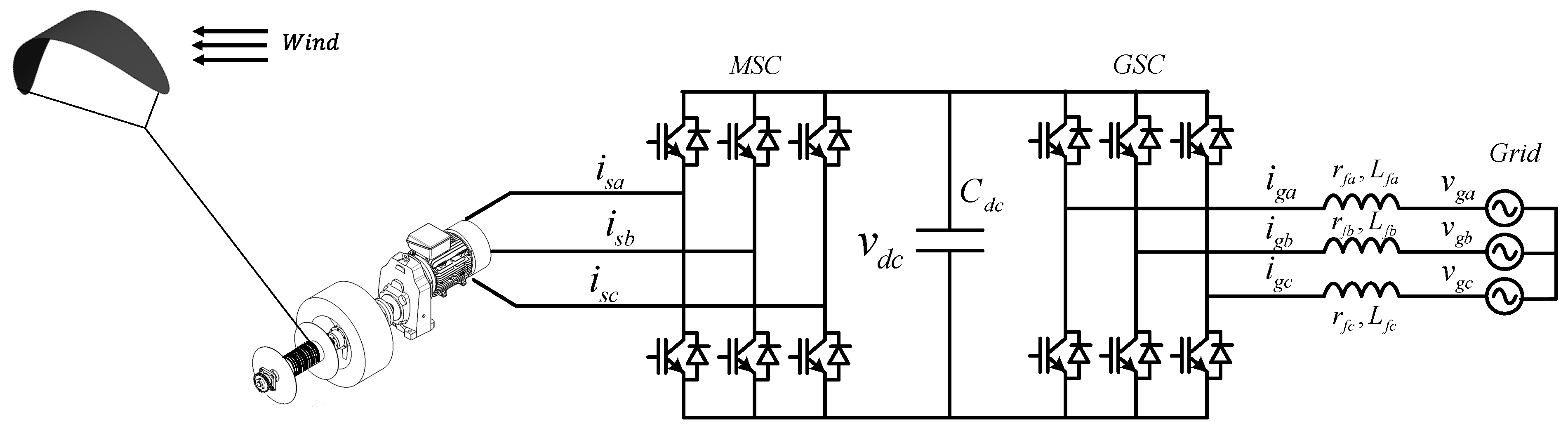
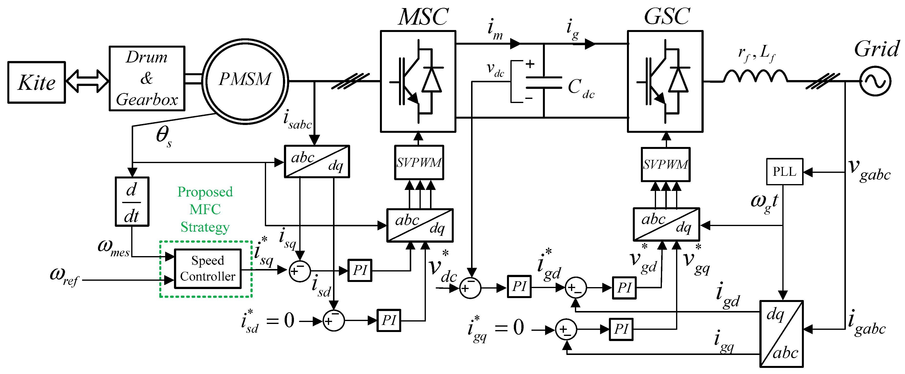
2. Power Kite Generator System Modeling

The operation of a wind-powered pumping kite generator presented in Figure 1 involves several phases to harness and efficiently convert wind energy. In the generation phase, the kite is maneuvered to rise in a crosswind motion, tracing an eight-trajectory pattern, which maximizes the extraction of energy from high-altitude winds [22]. Once the tether reaches its maximum length, the system transitions to the recovery phase. During recovery, the kite movement shifts to a non-crosswind motion, which is more effective in this phase [19], and the tether is reeled in consuming energy. This retraction prepares the kite for the next phase, forming a continuous cycle of alternating generation and recovery phases. The mechanical energy generated during the generation phase is transmitted via the tether and converted into electrical energy by an electrical generator on the ground.

The forces acting on the kite are given by

$$F=F_{grav}+F_{app}+F_{aer}+F_{trac}$$

(1)

where F_grav is the gravity force, F_app is the apparent force, and F_aer is the aerodynamic force, which depends on the effective wind speed W_e:

$$W_e=W_0-W_a$$

(2)

where W₀ is the wind speed, and W_a is the kite speed.

The aerodynamic force comprises two fundamental components: the lift force F_L and the drag force F_D, defined by [33].

$$F_L={\displaystyle \frac{1}{2}}{\rho }_{air}A{C}_L{\left|W_e\right|}^2$$

(3)

$$F_D={\displaystyle \frac{1}{2}}{\rho }_{air}A{C}_D{\left|W_e\right|}^2$$

(4)

where A is the kite surface, ρ_air is the air density, C_L is the lift coefficient, and C_D is the drag coefficient.

For the simplicity of analysis, it is assumed that inertial and apparent forces are negligible compared to aerodynamic forces. In addition, both the weight and the drag force of the tether are also neglected. Then, using a procedure similar to that described in [15,17,33,34], the traction force F_trac applied by the tether during the generation phase is found:

$$F_{trac}={\displaystyle \frac{1}{2}}{\rho }_{air}A{C}_L{E}^2{\left(1+{\displaystyle \frac{1}{E^2}}\right)}^{3/2}{\left|W_{e,r}\right|}^2$$

(5)

where E is the aerodynamic efficiency coefficient of the kite (E = C_L/C_D), and W_e,r is the effective wind speed along the cable direction. Posing the X axis aligned with wind speed, W_e,r can be defined as

$$W_{e,r}=W_{0}sin(\theta )cos(\phi )-{\dot{r}}^{trac}$$

(6)

where θ denotes the polar angle, φ represents the azimuth angle, and ${\dot{r}}^{trac}$ is the kite speed along the cable direction.

Additionally, the power generated can be provided via

$$P_{trac}={\displaystyle \frac{1}{2}}{\rho }_{air}A{C}_L{E}^2{\left(1+{\displaystyle \frac{1}{E^2}}\right)}^{3/2}{(W_{0}sin(\theta )cos(\phi )-{\dot{r}}^{trac})}^2{\dot{r}}^{trac}$$

(7)

The derivative of P_trac is calculated with respect to ${\dot{r}}^{trac}$ in order to obtain the optimal instantaneous value of the tether’s reeling out speed:

$${\displaystyle \frac{d{P}_{trac}}{d{\dot{r}}^{trac}}}={\displaystyle \frac{1}{2}}{\rho }_{air}A{C}_L{E}^2{\left(1+{\displaystyle \frac{1}{E^2}}\right)}^{3/2}\left[-2(W_{0}sin(\theta )cos(\phi )-\right.\left.{\dot{r}}^{trac}){\dot{r}}^{trac}+{(W_{0}sin(\theta )cos(\phi )-{\dot{r}}^{trac})}^2\right]$$

(8)

By solving for ${\dot{r}}^{trac}$ and setting the derivative to zero. There are two crucial points identified. Since one of them (W₀ sin(θ) cos(φ)) sets the power to zero, the optimal tether reeling out speed value is

$${\dot{r}}_{opt}^{trac}={\displaystyle \frac{W_{0}sin(\theta )cos(\phi )}{3}}$$

(9)

During the recovery phase, a wing glide maneuver is employed. The kite is controlled to align parallel to the tether, minimizing its aerodynamic lift, so the cable can be wound back fast with minimal energy consumption [35]. Additionally, in order to improve system efficiency during this phase, a higher reeling-in speed is used.

The PKGS is connected to the electrical grid through the power electronic conversion system illustrated in Figure 1. This system comprises several critical components that work to convert kinetic energy into electrical energy: a PMSM, which generates electrical power during generation phases and functions as a motor to reel in the cable during recovery phases; a machine-side converter (MSC) to regulate the PMSM current and torque, ensuring optimal shaft speed control to achieve MPPT; a grid-side converter (GSC) responsible for managing the power flow between the DC-link and the electrical grid, maintaining DC-link voltage stability, and controlling power exchange with the grid. Between the MSC and the GSC lies the DC-link capacitor, which maintains a stable voltage level and facilitates smooth power transfer. Finally, an inductive filter is employed to mitigate electrical noise and fluctuations of the power fed to the grid.

This work focuses on the control design for the MSC in a PKGS, specifically addressing the challenges of machine speed regulation. In the PKGS operation, the optimal tether reel-out speed during power generation phases must maintain a ratio of one-third of the wind speed component along the tether direction, as derived in (9). This reference speed contains periodic variations, as illustrated in Figure 2. Furthermore, the system must handle abrupt transitions between generation and recovery phases, where the machine reverses rotation direction to enable rapid tether retraction.

These operational requirements present two key control challenges:

• Precise tracking of a periodically varying reference speed during power generation phases.
• Ensuring stable transitions between generation and recovery phases.

Conventional PI controllers, typically designed for first- or second-order closed-loop response characteristics, perform adequately for step references but struggle with periodic reference tracking as encountered in PKGS applications. This tracking limitation directly affects power generation efficiency. While increasing controller gains could potentially improve dynamic response, this approach compromises system stability, leads to excessive control effort, and can introduce undesirable overshoots during phase transition phases without achieving satisfactory tracking performance during generation phases.

To address these limitations, this paper proposes an enhanced MFC approach incorporating a nonlinear hyperbolic tangent tracking differentiator. This novel approach aims to overcome both the periodic tracking and transition challenges inherent in PKGS operation.

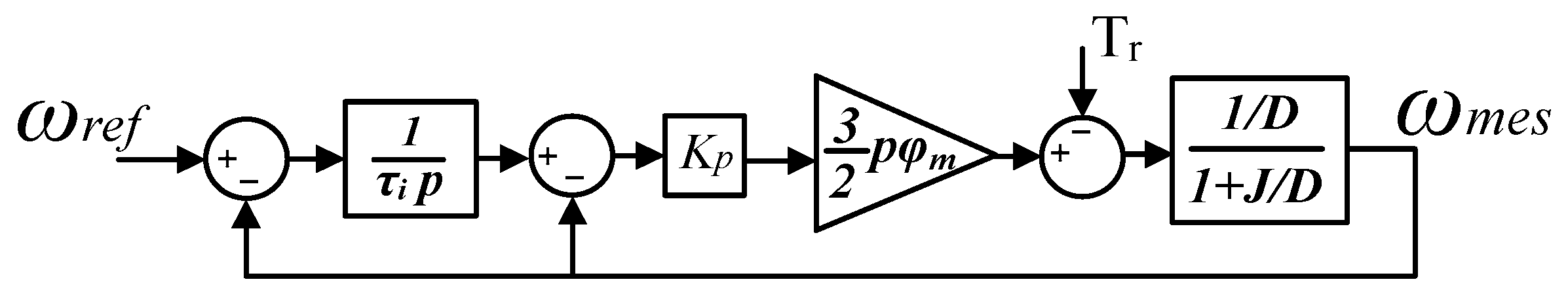
3. Model-Free Control

Typically, controller design relies on physics-based system models to enable dynamic feedback performance. Thus, conventional approaches depend heavily on model accuracy. However, MFC employs a different paradigm. The MFC methodology utilizes a numerical model with a minimal parameter set that is updated in real-time based only on input–output data measured from the system during operation.

3.1. Ultra Local Model

The fundamental concept of MFC comes from the assumption that mathematical model of a dynamic single-input–single-output (SISO) system with input u and output y can be approximated on a short time interval [t − T, t] by an ultra-local model equation [36].

$$y^{(n)}=F+\alpha u$$

(10)

where y represents the system output, n is the order of time derivation selected by the operator, u is the control input, F refers to a time-varying quantity that includes all exogenous disturbances and un-modeled dynamics such as nonlinearities and uncertainties, and α is a normalization factor chosen such as the quantities y⁽ⁿ⁾, F and αu have a similar order of magnitude.

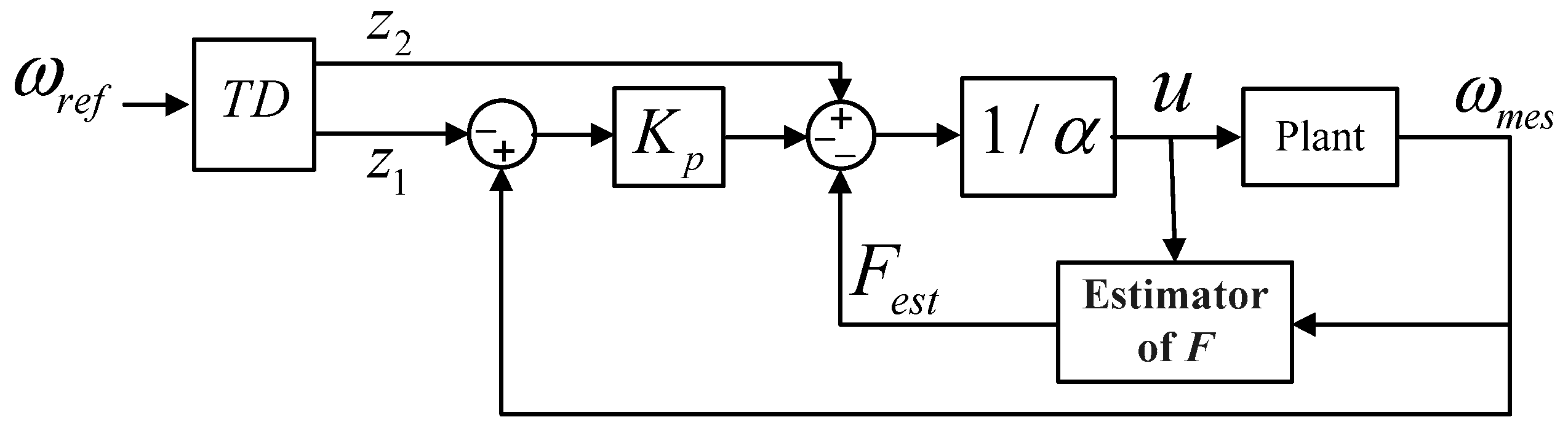
3.2. Intelligent Controllers

In this paper, the order of differentiation n of the ultra-local model is chosen as one. Thus, (10) can be expressed as

$$\dot{y}(t)=F(t)+\alpha u(t)$$

(11)

By closing the loop via the “intelligent Proportional” (iP) controller, the corresponding control input u in (11) is obtained as follows:

$$u(t)=-{\displaystyle \frac{F_{est}(t)-{\dot{y}}^{*}(t)+K_{p}e(t)}{\alpha }}$$

(12)

where F_est is an estimate of F, y* is the reference trajectory, e = y − y* is the tracking error, and K_p is the proportional gain.

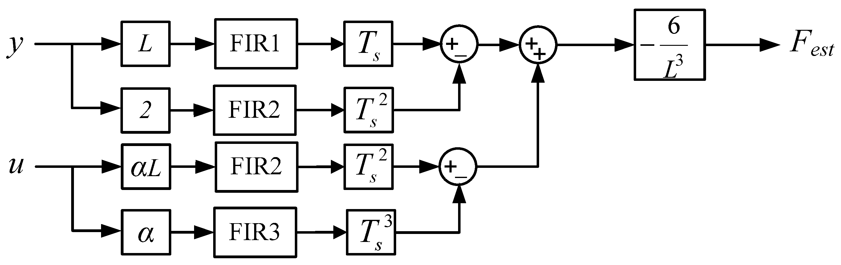
3.3. Online Estimation of F

Various techniques have been introduced in the literature for constructing an estimation of F [37]. In this work, the method developed in [25] is used. Where the unknown function F is approximated by a step function (a piecewise constant function) Φ, which can be reliably performed over a sufficiently small time interval. Therefore, Equation (11) becomes

$$\dot{y}(t)=\Phi +\alpha u(t)$$

(13)

By applying a Laplace transform (13), since Φ is a step function, it yields [25]

$$sY={\displaystyle \frac{\Phi }{s}}+\alpha U+y_0$$

(14)

where y₀ is the initial condition and s is the Laplace domain variable.

Both sides of (14) are multiplied by d/ds, thereby eliminating the initial condition and obtaining

$$Y+s{\displaystyle \frac{dY}{ds}}=-{\displaystyle \frac{\Phi }{s^2}}+\alpha {\displaystyle \frac{dU}{ds}}$$

(15)

By multiplying both sides of (15) by a sufficiently negative power of s to acquire a minimum of one integrator (${\displaystyle \frac{1}{s}}$) for each term in (15) in order to mitigate both noise and numerical computation inaccuracies in the output estimation, in this case s⁻², the following equation is thus obtained:

$${\displaystyle \frac{Y}{s^2}}+{\displaystyle \frac{dY}{sds}}=-{\displaystyle \frac{\Phi }{s^4}}+{\displaystyle \frac{\alpha }{s^2}}{\displaystyle \frac{dU}{ds}}$$

(16)

From (16), the estimate of Φ can be deduced, in the time domain, using inverse Laplace transforms, where [38]

$$s^{-1}F(s)\to {\displaystyle \underset{0}{\overset{t}{\int }}f(t)dt}$$

(17)

$$s^{-n}F(s)\to {\displaystyle {\int }^{(n)}f(t)dt}$$

(18)

$${\displaystyle \frac{d}{ds}}\to -t$$

(19)

$${\displaystyle \frac{d^n}{d{s}^n}}\to {(-1)}^n{t}^n$$

(20)

$${\displaystyle \frac{1}{s^n}}\to {\displaystyle \frac{t^{n-1}}{(n-1)!}}$$

(21)

From (18), we can obtain

$${\displaystyle \frac{Y}{s^2}}\to {\displaystyle {\int }^{(2)}y(t)dt}$$

(22)

and from (17) and (19), we obtain

$${\displaystyle \frac{dY}{sds}}\to {\displaystyle \int -ty(t)dt}$$

(23)

and from (21), we obtain

$${\displaystyle \frac{\Phi }{s^4}}\to {\displaystyle \frac{L^3}{6}}\Phi$$

(24)

and from (18) and (19), we obtain

$${\displaystyle \frac{\alpha }{s^2}}{\displaystyle \frac{dU}{ds}}\to \alpha {\displaystyle {\int }^{(2)}-tu(t)dt}$$

(25)

Using (22)–(25), we can transform (16) to a time domain as follows:

$${\displaystyle {\int }^{(2)}y(t)dt}-{\displaystyle \int ty(t)dt}=-{\displaystyle \frac{L^3}{6}}\Phi -\alpha {\displaystyle {\int }^{(2)}tu(t)dt}$$

(26)

Using Cauchy’s theorem in (27) to reduce multiple integrals into a simple one, we obtain

$${\displaystyle \underset{0}{\overset{T}{\int }}{\displaystyle \underset{0}{\overset{t_1}{\int }}\dots {\displaystyle \underset{0}{\overset{t_{\kappa -1}}{\int }}v(t_{\kappa }}}})d{t}_{\kappa }\dots d{t}_1={\displaystyle \underset{0}{\overset{T}{\int }}\frac{{(T-t)}^{\kappa -1}}{(\kappa -1)!}}v(t)dt$$

(27)

Applying (27) to the terms in (26) that contain multiple integrals, we obtain

$${\displaystyle \underset{0}{\overset{T}{\int }}{\displaystyle \underset{0}{\overset{t_1}{\int }}y(\sigma )d\sigma }}d{t}_1={\displaystyle \underset{0}{\overset{T}{\int }}\frac{(T-t)}{1!}}y(t)dt$$

(28)

$${\displaystyle \underset{0}{\overset{T}{\int }}{\displaystyle \underset{0}{\overset{t_1}{\int }}\sigma u(\sigma )d\sigma }}d{t}_1={\displaystyle \underset{0}{\overset{T}{\int }}\frac{(T-t)}{1!}}tu(t)dt$$

(29)

From (28) and (29), and by integrating during a quite small interval L, (26) becomes

$${\displaystyle \underset{t-L}{\overset{t}{\int }}(L-\sigma )y(\sigma )d\sigma }-{\displaystyle \underset{t-L}{\overset{t}{\int }}\sigma y(\sigma )d\sigma }=-{\displaystyle \frac{L^3}{6}}{F}_{est}-\alpha {\displaystyle \underset{t-L}{\overset{t}{\int }}\sigma (L-\sigma )u(\sigma )d\sigma }$$

(30)

Finally, we obtain the expression of F_est:

$$F_{est}=-{\displaystyle \frac{6}{L^3}}{\displaystyle \underset{t-L}{\overset{t}{\int }}((L-2\sigma )y(\sigma )+\alpha \sigma (L-\sigma )u(\sigma ))d\sigma }$$

(31)

In practice, the integral in (31) is substituted with finite impulse response (FIR) filters as presented in Figure 3.

The coefficients of the FIRs determined according to (31), and they are as follows:

$$\mathrm{FIR}1=\left[\begin{array}{ccccc}1& 1& 1& \dots & 1\end{array}\right]$$

(32)

$$\mathrm{FIR}2=\left[\begin{array}{ccccc}1& 2& 3& \dots & N\end{array}\right]$$

(33)

$$\mathrm{FIR}3=\left[\begin{array}{ccccc}1& 4& 9& \dots & N^2\end{array}\right]$$

(34)

where N denotes the number of samples used in the FIR, such as L = N × T_s, and T_s is the sampling time.

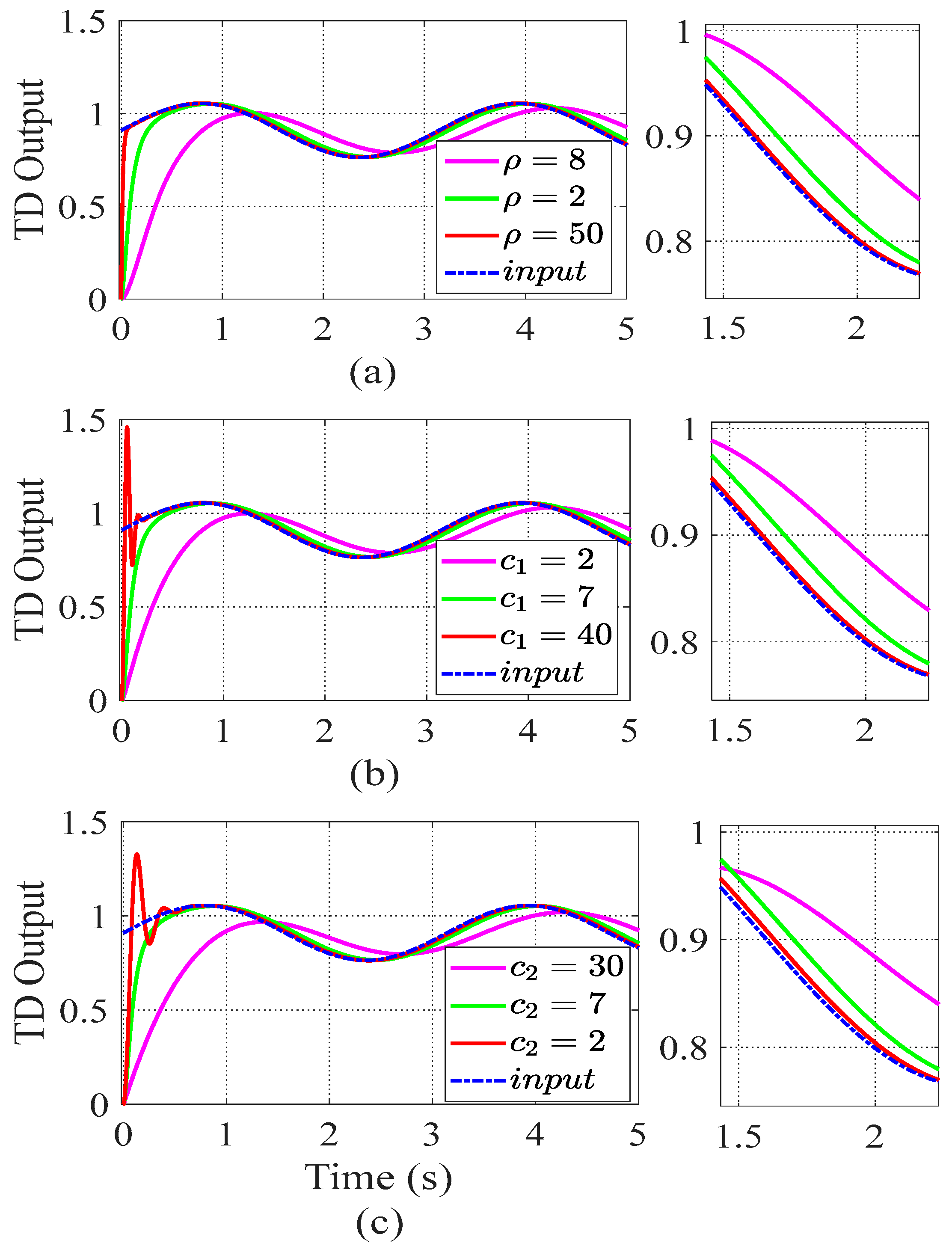
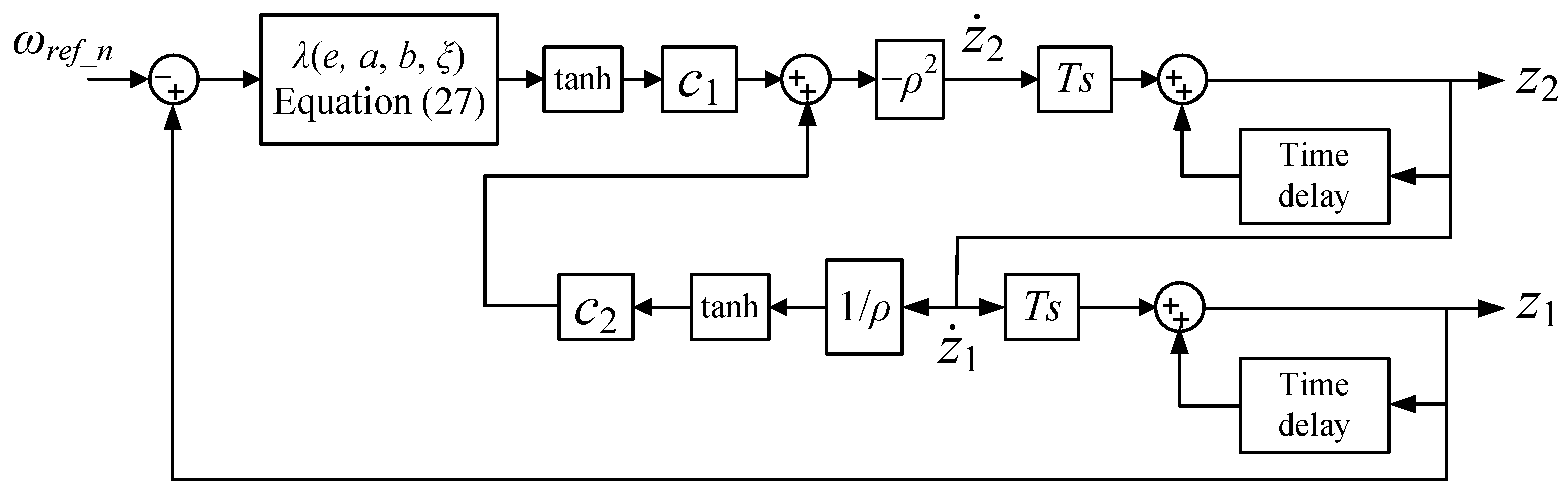
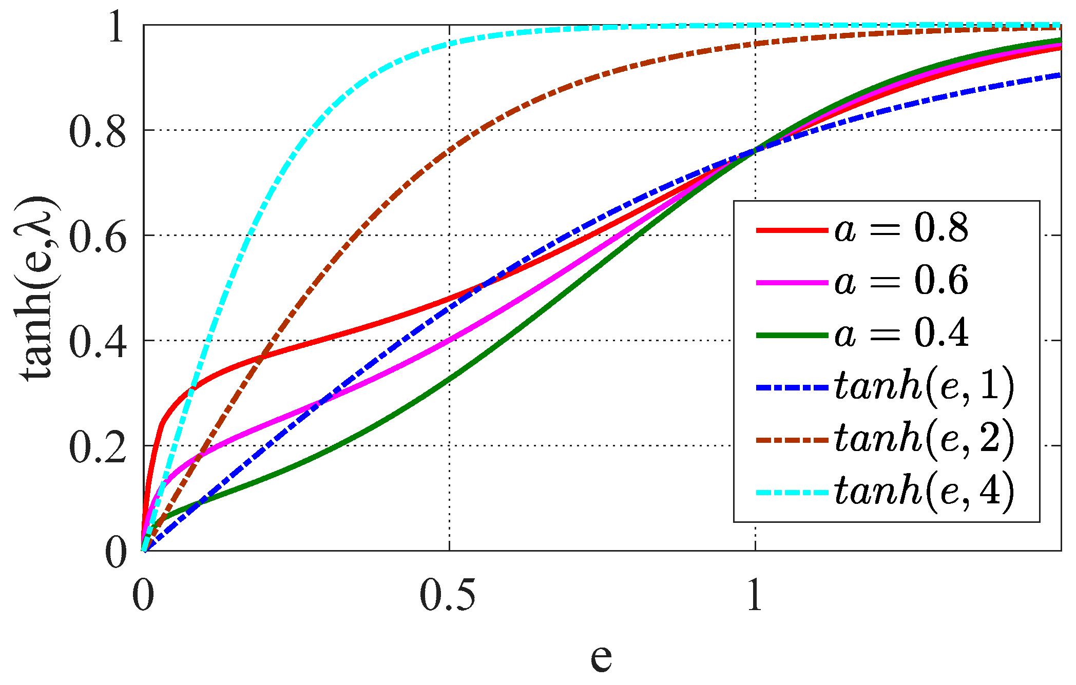
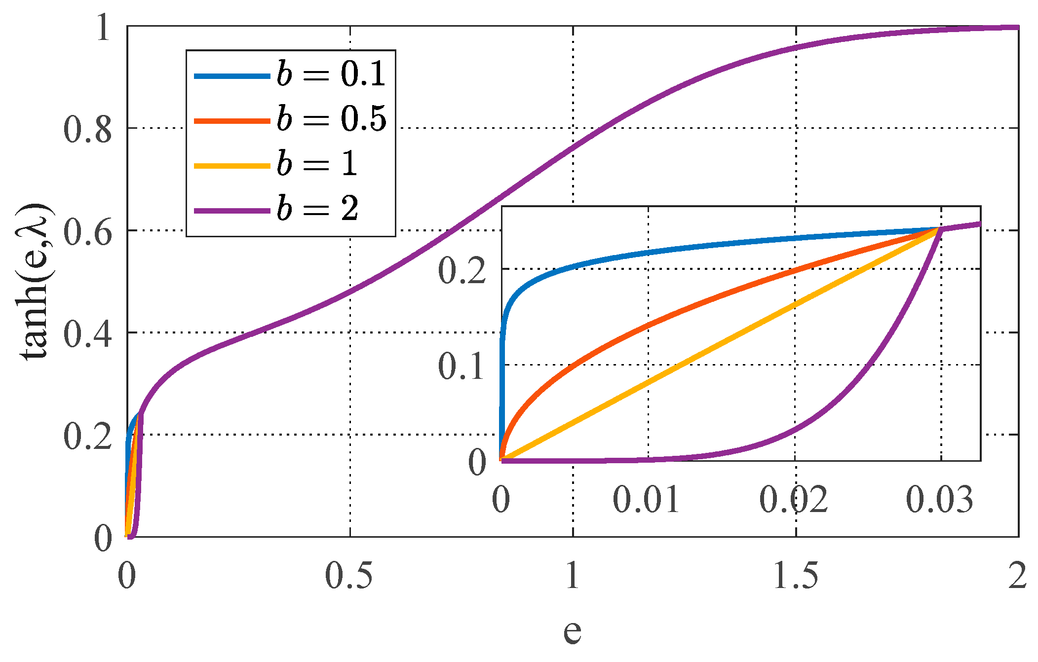
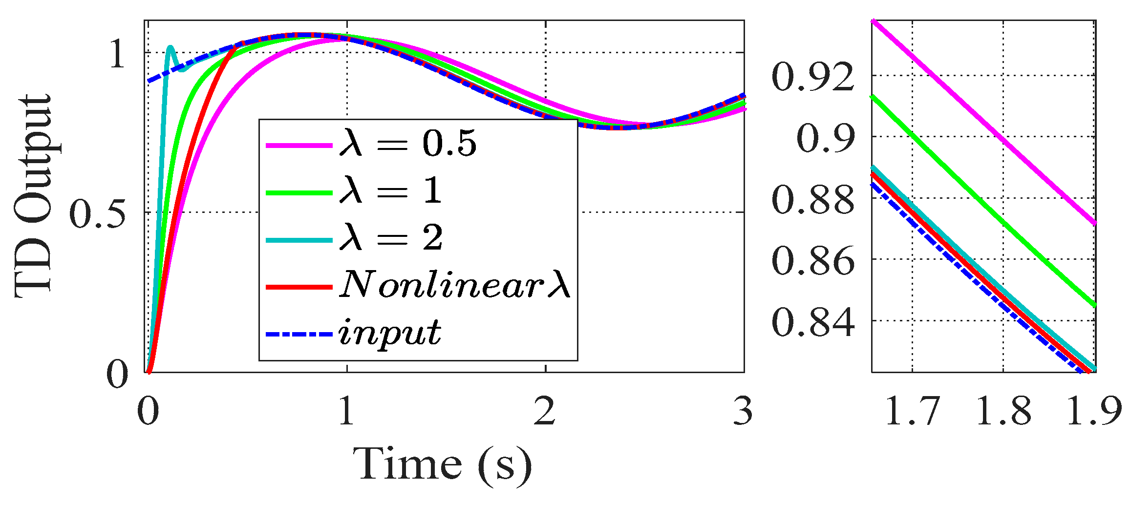
3.4. Tracking Differentiator Design Based on Hyperbolic Tangent Function

In MFC, both the reference signal and its derivative are essential components of the control law. However, the direct calculation of the derivative can lead to significant challenges, particularly when the reference changes abruptly, such as transition phases in a PKGS. In these cases, the derivative may yield excessively large values, potentially leading to the instability of the system. While the derivative of the trajectory is often set to zero when dealing with step responses, this approach is not suitable for systems with varying speed references, such as a PKGS during the traction phase. To address these issues and ensure robust control, the integration of a tracking differentiator into the MFC framework is proposed in this work.

The TD developed in this work is based on the improved hyperbolic tangent function proposed in [39]. The hyperbolic tangent function is derived from the ratio of the hyperbolic sine (sinh) and the hyperbolic cosine (cosh) functions. It produces a smooth, continuous curve with distinct saturated regions. Near the origin, the hyperbolic tangent can be approximated as a linear function, despite its overall nonlinear nature. It is expressed as

$$tanh(x)={\displaystyle \frac{e^x-e^{-x}}{e^x+e^{-x}}}$$

(35)

Equation (35) can be formed as

$$tanh(x)=1-{\displaystyle \frac{2}{e^{2x}+1}}$$

(36)

As can be deduced from (36), the curve of the tanh is a strictly monotone rising function with upper and lower bounds of 1 and −1 for the saturation value. To modify the approximate linear range close to the origin, the exponential component λ is introduced in Formula (36), with the resulting function shown in Figure 4, and the new formula is obtained as follows:

$$tanh(x,\lambda )=1-{\displaystyle \frac{2}{e^{2\lambda x}+1}}$$

(37)

Consider the following second-order system,

$$\left\{\begin{array}{l}{\dot{z}}_1=z_2\\ {\dot{z}}_2=f(z_1,z_2,v)\end{array}\right.$$

(38)

where f is the nonlinear hyperbolic tangent function given by

$$f(z_1,z_2)=-{\rho }^2\left(c_{1}tanh\left(z_1(t)-v(t)\right)+c_{2}tanh\left({\displaystyle \frac{z_2(t)}{\rho }}\right)\right)$$

(39)

where v(t) represents the input, ρ and c₁ are utilized to adjust the tracking speed, c₂ is associated with the differential effect.

Figure 5 shows the TD output for different parameter values. It can be seen that for low values of ρ and c₁, and high values of c₂, there is a noticeable delay between the TD output and the input signal. As ρ and c₁ increase and c₂ decreases, this delay gradually diminishes, resulting in a faster system response. However, this improvement in delay reduction comes with trade-offs. When the parameters reach values that effectively eliminate the delay, the TD response speed can exceed the tracking capabilities of the real system, which can have a negative impact on system stability, significantly increase the required control effort, and potentially cause overshoots in the system response.

To address this compromise, a nonlinear function is introduced for adjusting the approximate linear range of the hyperbolic tangent function. Consequently, the system becomes

$$f(z_1,z_2)=-{\rho }^2\left(c_{1}tanh\left(\lambda e(t)\right)+c_{2}tanh\left({\displaystyle \frac{z_2(t)}{\rho }}\right)\right)$$

(40)

where e is the normalized error between z₁ and v(t), and λ is a nonlinear function defined as follows:

$$\lambda (e,a,b,\xi )=\left\{\begin{array}{cc}{\displaystyle \frac{{\left|e\right|}^b}{{\xi }^{b-a}}}\mathrm{sign}(e)& \left|e\right|\le \xi \\ {\left|e\right|}^a\mathrm{sign}(e)& \left|e\right|>\xi \end{array}\right.$$

(41)

a, b, and ξ are parameters which can be adjusted to meet the required performance levels.

Figure 6 illustrates the diagram of the proposed TD based on Equations (38), (40) and (41), where ω_{ref_n} represents the normalized rotational speed.

The traditional hyperbolic tangent function commonly used in control systems provides a smooth, symmetric curve with a linear region near the origin and saturation at the extremes. Despite being efficient in many situations, it might not be the best option due to the previously mentioned trade-off, and to enhance tracking accuracy during periodic phases (where errors are typically small) by increasing the gain parameter λ, the system must compromise on the stability of the transition response, potentially resulting in faster, less controlled transitions. The proposed function, described in (40), introduces a nonlinear modification to the error before passing it through the hyperbolic tangent function. To ensure good tracking accuracy in periodic phase, this function has to amplify the tracking error when it is near the equilibrium point. Conversely, it scales down the error when it is far from the equilibrium in order to have a stable transition response that respects the physical limit of the system.

Figure 7 and Figure 8 illustrate the influence of parameters a and b on the nonlinear gain function λ. As depicted, a and b primarily affect the slope of the function in regions of small errors. Smaller values of a and larger values of b result in a low slope near the origin, while larger values of a and smaller values of b increase the sensitivity to small errors. In our case, we are looking for a higher slope in order to enhance accuracy in steady-state phases without noise amplification. The parameter ξ defines the threshold separating small and large error regions, marking the boundary where the gain function’s behavior transitions. By appropriately adjusting these parameters, we can fine-tune the system’s accuracy during steady-state operation when errors are small (traction phases) and control the aggressiveness of the system in correcting large deviations and guarantee a smooth transition between the two phases, all without compromising noise sensitivity.

Figure 9 illustrates the performance advantages offered by the proposed TD incorporating a nonlinear λ. This approach demonstrates the highest tracking accuracy compared to TDs with constant λ, even with high values. Notably, this enhanced precision does not come at the cost of dynamic response quality. The figure reveals that despite achieving the best tracking accuracy, the proposed TD neither exhibits the fastest response nor produces overshoots. This balanced performance underscores a key benefit of the proposed TD: it simultaneously delivers a stable transition response that respects the system’s physical limitations and maintains excellent tracking accuracy during periodic phases. Such dual optimization represents a significant advancement in control system design, offering a solution that does not compromise between transition stability and steady-state precision.

The proposed MFC (PMFC) scheme is shown in Figure 10.

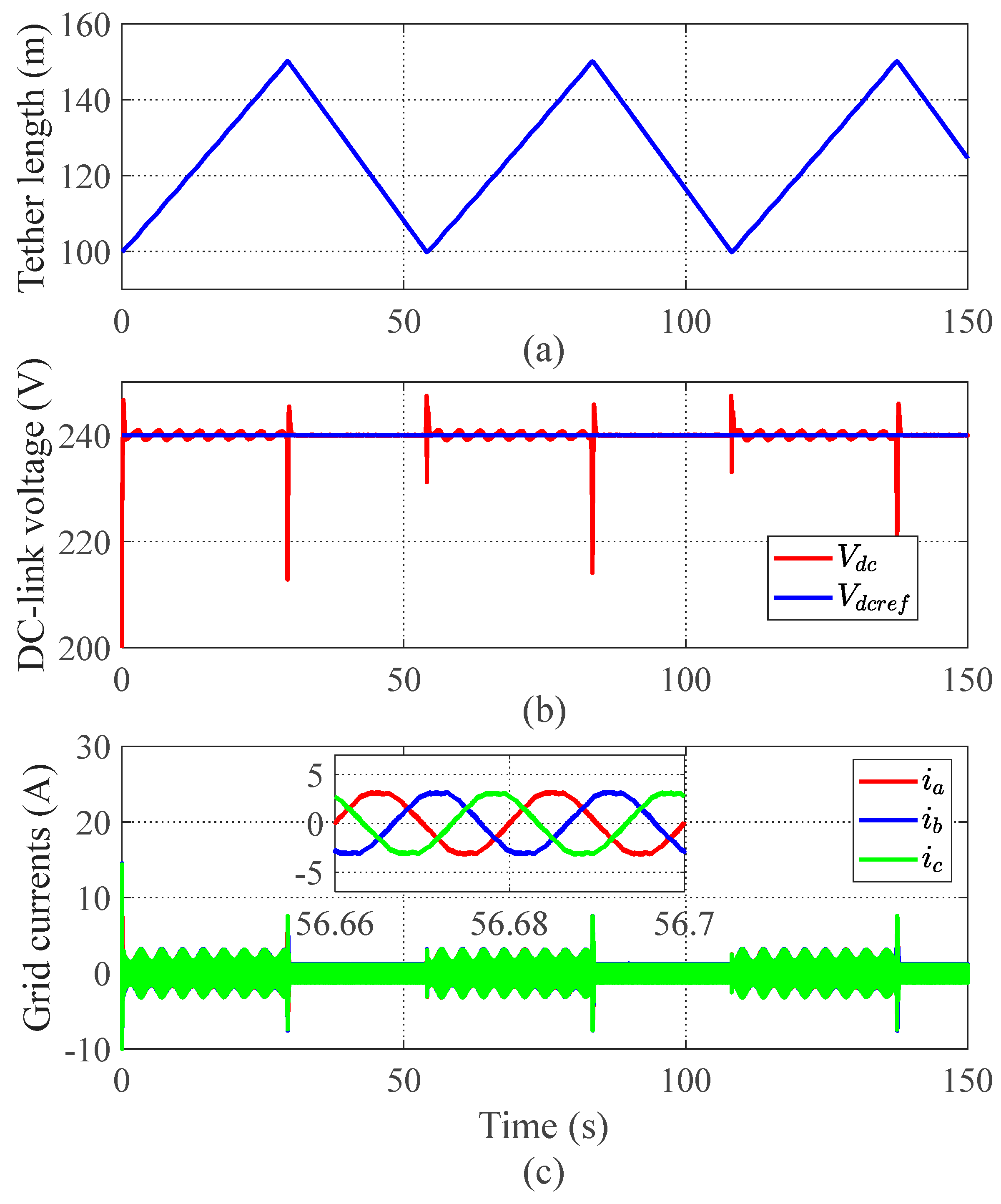
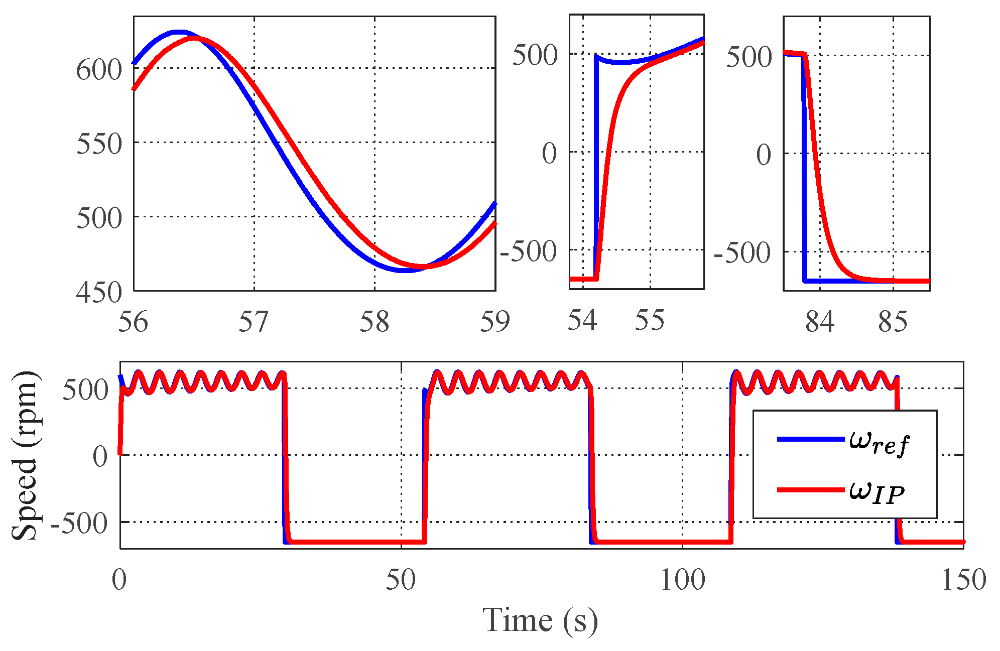
4. Simulation Results

To assess the effectiveness of the proposed MFC (PMFC) technique, simulations were conducted using the MATLAB/Simulink environment. The simulations are based on the system depicted in Figure 11. The power conversion system’s parameters are detailed in

Table 1. Kite generator system parameters.

Parameters	Symbol	Value
Kite’s area	A	3 m2
Air density	ρair	1.225 kg/${\mathrm{m}}^3$
Lift coefficient	CL	1
Drag coefficient	CD	0.33
Pole pair number	p	2
System total inertia	J	0.03 kg m2
Viscous damping	D	0.005 N.m.s
Machine inductance	Ls	6 mH
Machine resistance	Rs	0.2 Ω
Machine flux linkage	φm	0.6 Wb
DC-link capacitance	C	4700 μF
Grid-side filter inductance	Lf	20 mH
Grid-side filter resistance	Rf	0.5 Ω
Carrier frequency	Fc	5 kHz
Sampling time	TS	5 × 10−6 s

.

Here, the PMFC strategy is being compared to the integral–proportional (IP) regulator depicted in Figure 12, and with the conventional MFC without the TD.

The IP controller is chosen over the PI controller to eliminate the zero typically present in the closed-loop transfer function of PI controllers in order to mitigate overshoot during transient phases [40]. The IP controller parameters are obtained by synthesizing the closed-loop system with a response of a second-order system of the following canonical form.

The parameters of the integral–proportional (IP) controller are obtained by synthesizing the closed-loop system response to match a canonical second-order system form [15].

$$H\left(s\right)={\displaystyle \frac{1}{1+\frac{2m}{{\omega }_n}s+\frac{1}{{\omega }_n^2}{s}^2}}$$

(42)

This approach ensures the IP controller is designed to deliver the desired transient characteristics, such as natural frequency ω_n and damping ratio m. Then, the proportional and integral parts are obtained as follows:

• $K_{p\omega }={\displaystyle \frac{2D}{3p{\phi }_m}}\left(2m{\tau }_m{\omega }_n-1\right)$
• ${\tau }_{iw}={\displaystyle \frac{3K_{pw}p{\phi }_m}{2D{\tau }_m{\omega }_n^2 }}.$

where τ_m = J/D, and φ_m is the machine flux linkage. The parameters for IP controller are then selected as ω_n = 10 and m = 1.1, providing the desired system dynamics.

The gains of the MFC are manually tuned following the procedure outlined in [26]. The tuning process begins by selecting a very large α and a high K_p, ensuring a minimal steady-state error. Next, α is gradually reduced to achieve a quick, oscillatory response, enhancing the system’s speed. Finally, K_p is decreased incrementally to stabilize the system, balancing responsiveness and stability.

To ensure a fair and meaningful comparison of the control strategies, the parameters for the MFC were adjusted, before introducing the TD, so that the system exhibits the same dynamic response as when the IP controller is used with its selected parameters. After tuning, the MFC parameters were determined to be K_p = 8 and α = 1.5 × 10⁵.

The TD parameters are chosen as ρ = 40, c₁ = 2, c₂ = 20, a = 0.4, b = 0.5, and ξ = 0.03.

For the DC-link and current regulation within the GSC control, as well as for the inner current loops in the MSC control, the control strategy employs the classical PI control method. This configuration is depicted in Figure 11.

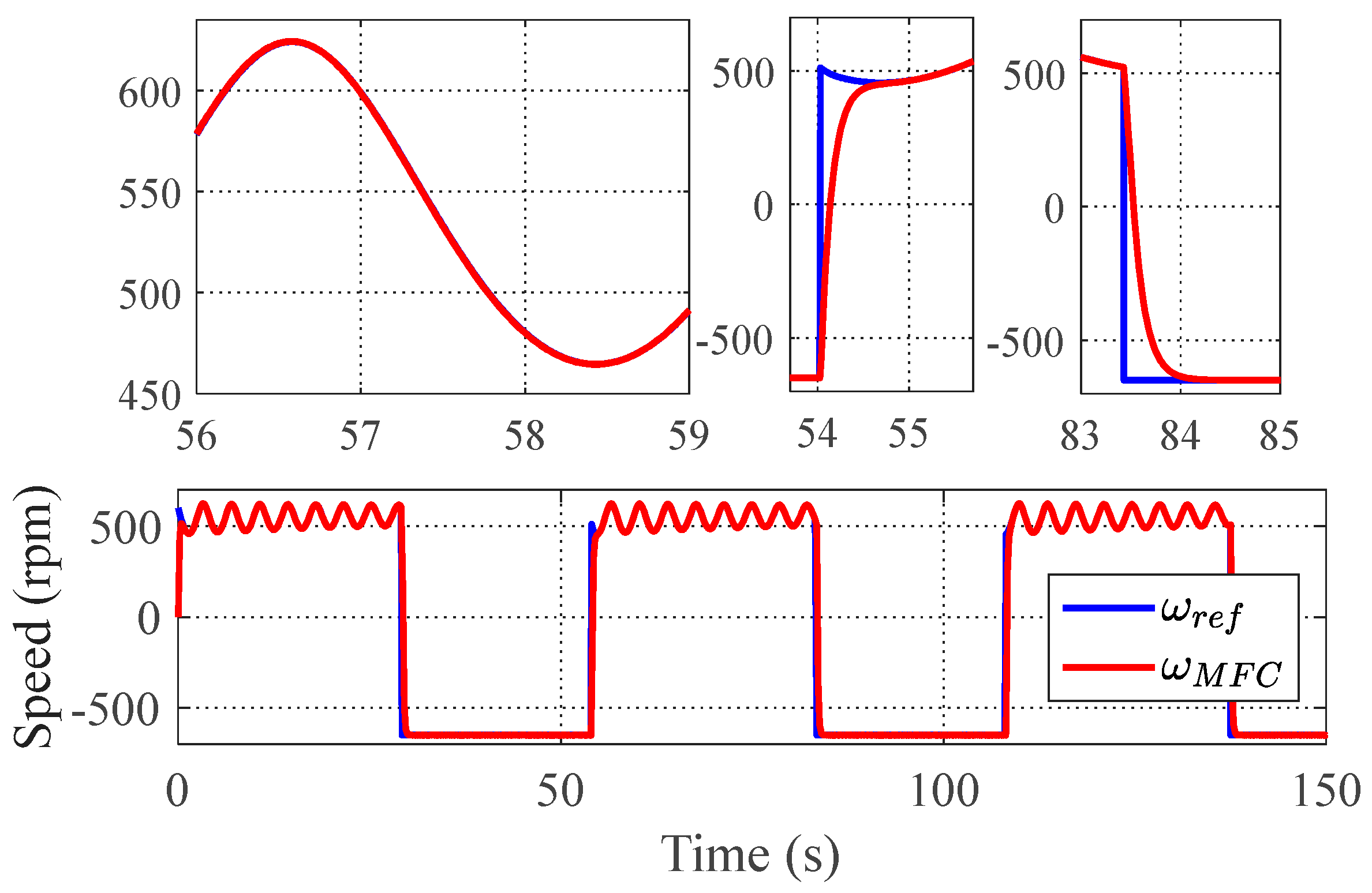
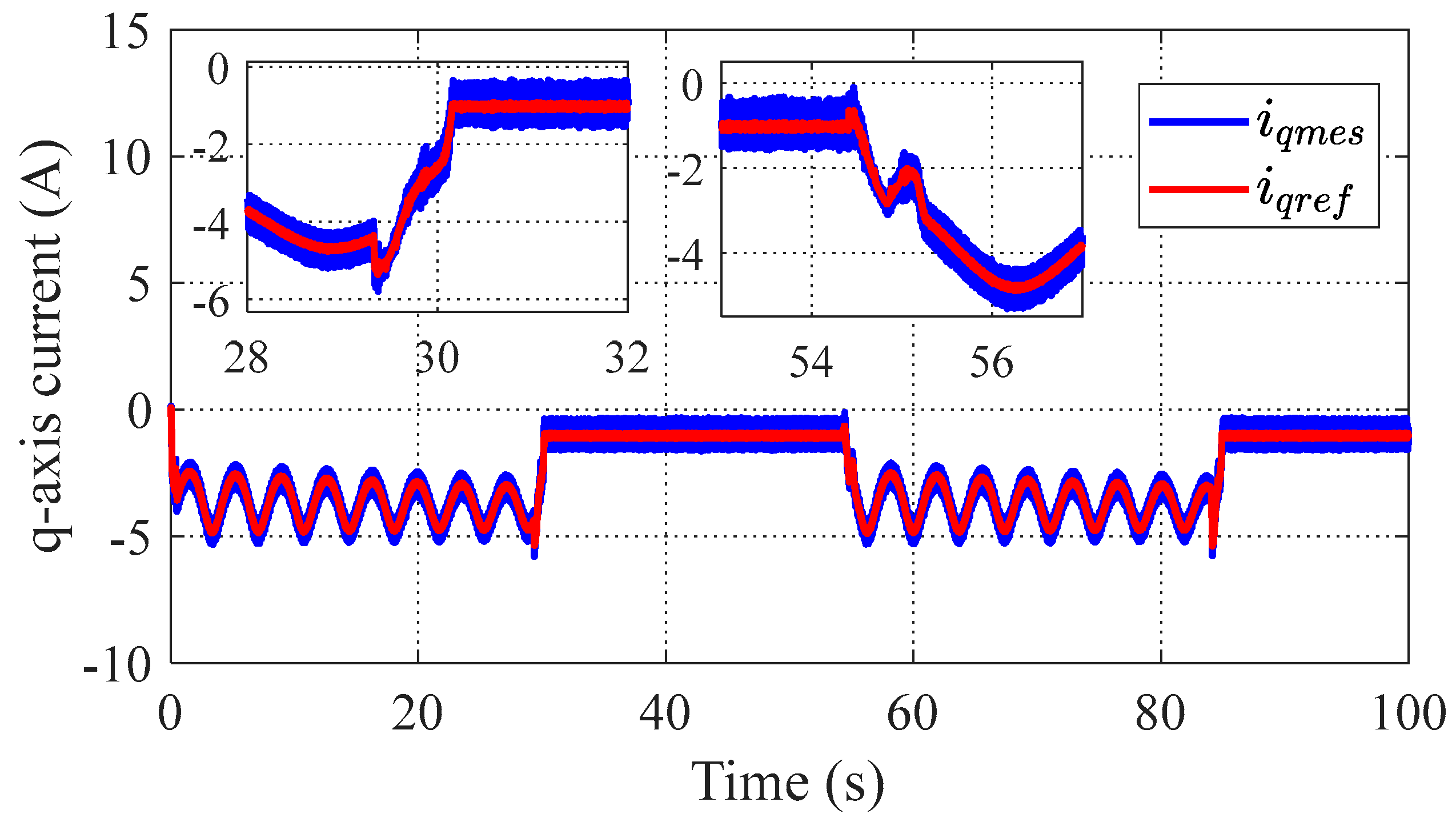
4.1. Tracking Performance

To validate the effectiveness of the proposed control strategy, multiple traction-recovery cycles are conducted at a wind speed of 8 m/s. The cable length ranges from 100 m to 150 m, as illustrated in Figure 13a. Figure 13b,c illustrate the DC-link voltage and the grid currents throughout the cycles.

In the traction phase, the machine rotor speed is controlled so that the tether’s reeling-out speed is 1/3 of the wind speed component along the tether direction, which is its optimal value [21]. A fast reel-in speed is used in the recovery phase for more efficiency of the system.

A comparative analysis of the three control methods reveals distinct performance characteristics. The IP controller, as observed in Figure 14, offers stable transitions between traction and recovery phases, with relatively small peaks in the controller output (q-axis current) as shown in Figure 15. However, its tracking performance in the traction phase is poor, exhibiting a noticeable delay because of the periodic component in speed reference.

The conventional MFC, illustrated in Figure 16, demonstrates good tracking performance for periodically changing speeds during the traction phases. However, it faces challenges during transition phases, where the controller output becomes excessively high due to derivative action. As a result, rather than achieving true dynamic control, the system dynamics are constrained by the saturation limits [−10,10], as shown in Figure 17.

In contrast, the PMFC, as shown in Figure 18 and Figure 19, achieves excellent tracking performance for periodically changing speeds in the traction phase while simultaneously maintaining stable transition phases. Notably, the PMFC’s output remains smooth with smaller peaks than the IP controller, indicating more efficient, controlled, and stable operation throughout.

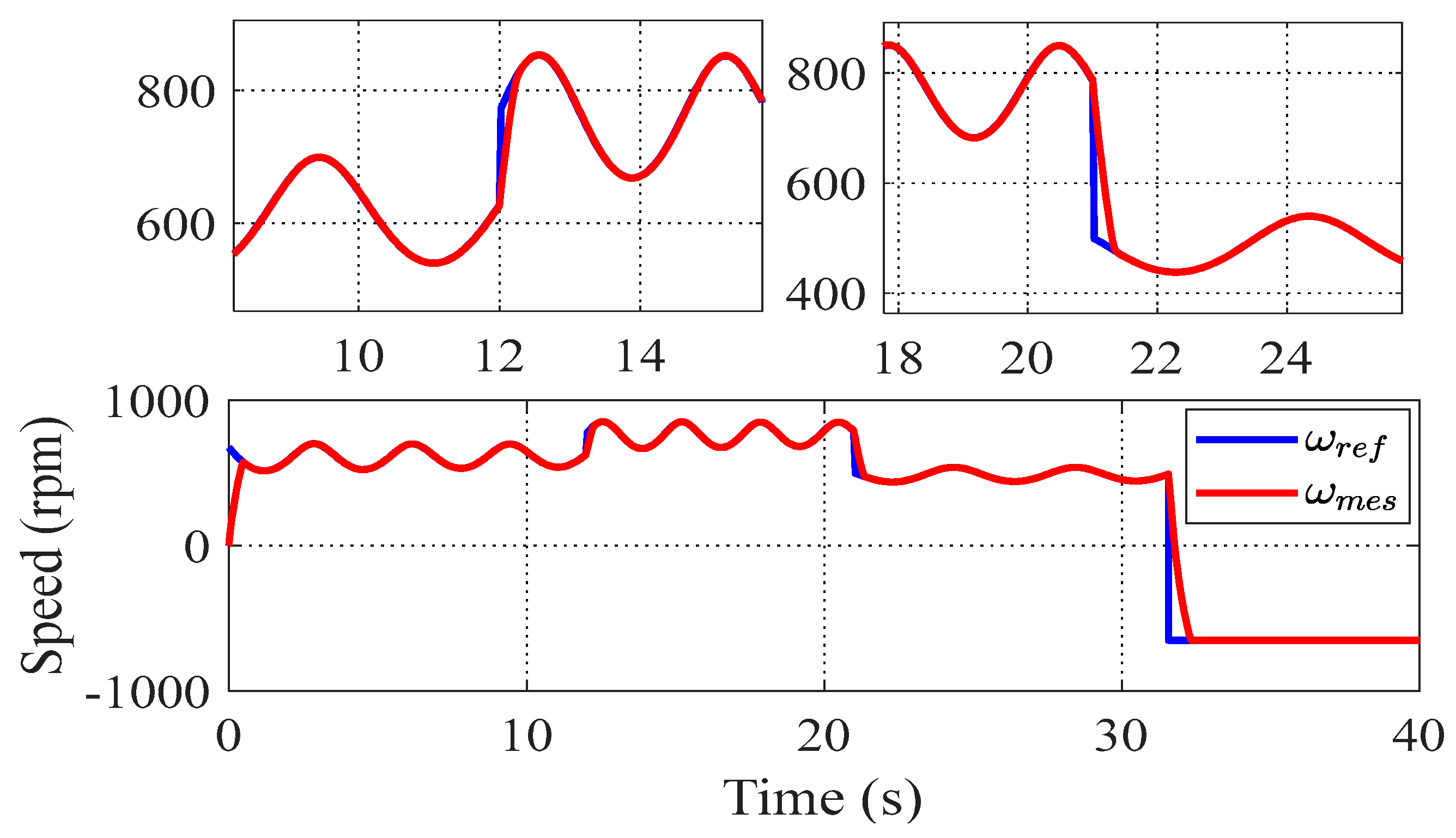
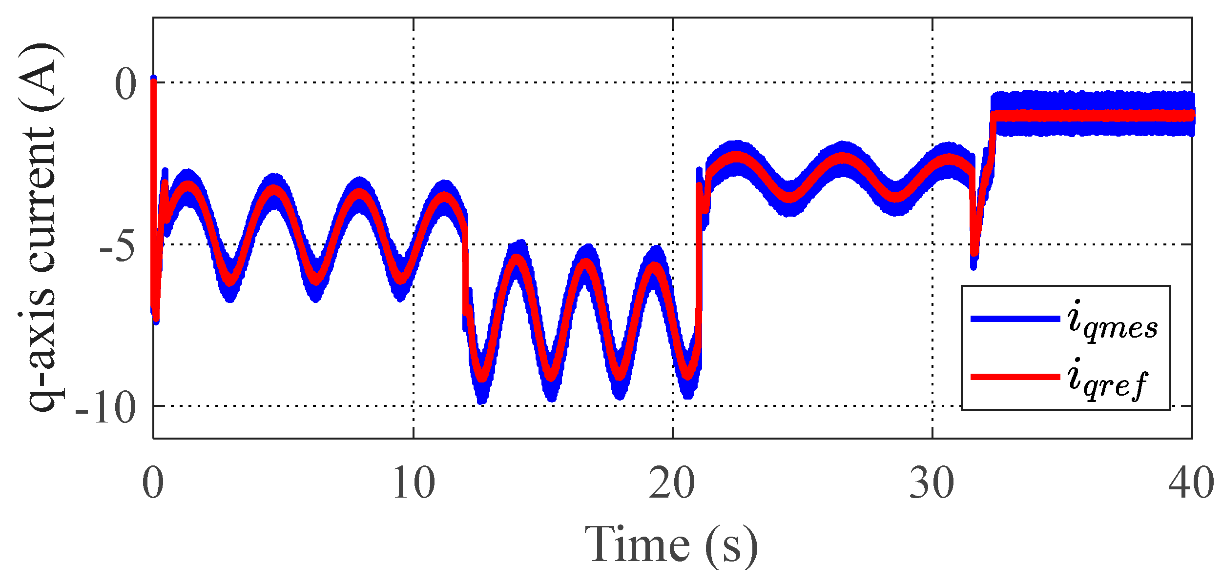
4.2. Scalability in Varying Environmental Conditions

The scalability of the proposed system under varying environmental conditions is tested to evaluate the PMFC adaptability to different wind profiles and its effectiveness across different kite dimensions.

The system’s response to dynamic wind conditions was evaluated using a time-varying wind speed profile, as illustrated in Figure 20. The simulation results, presented in Figure 21 and Figure 22, demonstrate the controller’s robust performance under changing wind conditions. The control system provided very good tracking across the entire wind speed range, with speed transitions remaining smooth and controlled while meeting the desired dynamic response characteristics. The controller demonstrated the ability to automatically adjust its output without requiring parameter recalibration.

To evaluate the control strategy scalability to different PKGS sizes, we conducted simulations by varying the kite’s area to 6 m² with a wind speed of 8 m/s. The results, shown in Figure 23 and Figure 24, reveal that the control performance remained consistent across different kite sizes, with no controller retuning required when scaling the kite area. The system maintained stable operation despite the significant change in aerodynamic forces, while control signal magnitudes appropriately scaled with the change in kite size. This size-independent performance represents one of the core advantages of the MFC approach, and since the controller does not rely on system parameters or model-based calculations, it naturally adapts to changes in the physical system’s scale.

5. Conclusions

This paper presents a novel approach for addressing the control challenges inherent in a grid-connected wind-powered PKGS. The unique operational characteristics of this technology necessitate a robust and adaptive control strategy that goes beyond conventional methods. An enhanced MFC strategy, specifically tailored for PKGS applications, has therefore been designed. By integrating a nonlinear hyperbolic tangent TD into the MFC framework, we have successfully resolved the compromise between achieving stable transition phases and maintaining excellent tracking performance during generation phases. This innovative approach addresses the limitations of conventional MFC when dealing with step references and periodic speed variations, which are critical aspects of a PKGS operation.

A comparative analysis conducted through simulations demonstrated the superiority of the proposed method over traditional control strategies such as IP controllers and conventional MFC. The PMFC offers enhanced tracking accuracy during the traction phase, crucial for maximizing power generation. Additionally, by eliminating peaks in the control output, the method leads to more efficient, reliable, and stable transitions between traction and recovery phases.

The simulation results also demonstrated the robust scalability of the proposed control system across varying operational conditions. The controller demonstrated consistent performance under varying wind speed profiles and kite sizes, ensuring reliable tracking accuracy and smooth speed transitions throughout the tested range. This inherent adaptability, attributed to the MFC approach, suggests the promising potential of the system’s deployment across different PKGS installations and operating environments.

These improvements collectively contribute to optimizing the power generation efficiency of PKGS while maintaining system stability and reliability.

Although the simulation tool used for the validation of the proposed control strategies and the developed mathematical models has given very promising results, experimental validation in real conditions remains essential. Future work will focus on developing a dedicated experimental test bed to evaluate the performance of the proposed control algorithms under real-world conditions. The experimental phase will enable the validation of several critical aspects of our work. It will allow the evaluation of the hyperbolic tangent tracking differentiator robustness under real sensor noise and measurement uncertainties, as well as the assessment of the control system response to machine dynamics and wind disturbances. This testing will also allow the determination of the practical computational requirements and implementation constraints while validating the robust performances and scalability findings suggested by the simulation results. This experimental validation will provide valuable insights for bridging the gap between theoretical analysis and practical implementation, potentially revealing additional considerations not captured in the simulation environment.

References

1. Tang, Z.; Yang, Y.; Blaabjerg, F. Power electronics: The enabling technology for renewable energy integration. CSEE J. Power Energy Syst. 2021, 8, 39–52. [Google Scholar]
2. Badihi, H.; Zhang, Y.; Jiang, B.; Pillay, P.; Rakheja, S. A comprehensive review on signal-based and model-based condition monitoring of wind turbines: Fault diagnosis and lifetime prognosis. Proc. IEEE 2022, 110, 754–806. [Google Scholar] [CrossRef]
3. Saberi, S.; Rezaie, B. Robust adaptive direct speed control of PMSG-based airborne wind energy system using FCS-MPC method. ISA Trans. 2022, 131, 43–60. [Google Scholar] [CrossRef]
4. Vermillion, C.; Cobb, M.; Fagiano, L.; Leuthold, R.; Diehl, M.; Smith, R.S.; Wood, T.A.; Rapp, S.; Schmehl, R.; Olinger, D. Electricity in the air: Insights from two decades of advanced control research and experimental flight testing of airborne wind energy systems. Annu. Rev. Control 2021, 52, 330–357. [Google Scholar] [CrossRef]
5. Malz, E.C.; Verendel, V.; Gros, S. Computing the power profiles for an Airborne Wind Energy system based on large-scale wind data. Renew. Energy 2020, 162, 766–778. [Google Scholar] [CrossRef]
6. Malz, E.C.; Walter, V.; Göransson, L.; Gros, S. The value of airborne wind energy to the electricity system. Wind Energy 2022, 25, 281–299. [Google Scholar] [CrossRef]
7. Schmidt, E.; de Oliveira, M.D.L.C.; da Silva, R.S.; Fagiano, L.; Neto, A.T. In-flight estimation of the aerodynamics of tethered wings for airborne wind energy. IEEE Trans. Control Syst. Technol. 2019, 28, 1309–1322. [Google Scholar] [CrossRef]
8. Akberali, A.F.K.; Kheiri, M.; Bourgault, F. Generalized aerodynamic models for crosswind kite power systems. J. Wind Eng. Ind. Aerodyn. 2021, 215, 104664. [Google Scholar] [CrossRef]
9. Yan, C.; Zhang, H. Analysis of the work performance of the lift mode crosswind kite power system based on aerodynamic parameters. Energy Rep. 2022, 8, 40–52. [Google Scholar] [CrossRef]
10. Zempoalteca-Jimenez, M.-A.; Castro-Linares, R.; Alvarez-Gallegos, J. Trajectory Tracking Flight Control of a Tethered Kite Using a Passive Sliding Mode Approach. IEEE Lat. Am. Trans. 2021, 20, 133–140. [Google Scholar] [CrossRef]
11. Costello, S.; François, G.; Bonvin, D. Real-time optimizing control of an experimental crosswind power kite. IEEE Trans. Control Syst. Technol. 2017, 26, 507–522. [Google Scholar] [CrossRef]
12. Bari, S.; Khan, M.U. Sliding mode control for autonomous flight of tethered kite under varying wind speed conditions. In Proceedings of the 2020 17th International Bhurban Conference on Applied Sciences and Technology (IBCAST), Islamabad, Pakistan, 14–18 January 2020; pp. 315–320. [Google Scholar]
13. Todeschini, D.; Fagiano, L.; Micheli, C.; Cattano, A. Control of a rigid wing pumping Airborne Wind Energy system in all operational phases. Control Eng. Pract. 2021, 111, 104794. [Google Scholar] [CrossRef]
14. Siddiqui, A.; Borek, J.; Vermillion, C. A Fused Gaussian Process Modeling and Model Predictive Control Framework for Real-Time Path Adaptation of an Airborne Wind Energy System. IEEE Trans. Control Syst. Technol. 2022, 31, 475–482. [Google Scholar] [CrossRef]
15. Belguedri, M.; Benrabah, A.; Khoucha, F.; Benbouzid, M.; Benmansour, K. An improved uncertainty and disturbance estimator-based speed control for grid-connected pumping kite wind generator. Control Eng. Pract. 2024, 143, 105795. [Google Scholar] [CrossRef]
16. Schechner, K.; Bauer, F.; Hackl, C.M. Nonlinear DC-link PI control for airborne wind energy systems during pumping mode. In Airborne Wind Energy: Advances in Technology Development and Research; Springer: Singapore, 2018; pp. 241–276. [Google Scholar]
17. Belguedri, M.; Amirat, Y.; Benrabah, A.; Khoucha, F.; Benbouzid, M.; Benmansour, K. Active Disturbance Rejection Control with a Cascaded Extended State Observer for Pumping Kite Generator Systems Robust DC-Link Voltage Control. IEEE Trans. Energy Convers. 2024, 1–12. [Google Scholar] [CrossRef]
18. Zhao, Y.; Wei, C.; Zhang, Z.; Qiao, W. A review on position/speed sensorless control for permanent-magnet synchronous machine-based wind energy conversion systems. IEEE J. Emerg. Sel. Top. Power Electron. 2013, 1, 203–216. [Google Scholar] [CrossRef]
19. Berra, A.; Fagiano, L. An optimal reeling control strategy for pumping airborne wind energy systems without wind speed feedback. In Proceedings of the 2021 European Control Conference (ECC), Rotterdam, The Netherlands, 29 June–2 July 2021; pp. 1199–1204. [Google Scholar]
20. Argatov, I.; Silvennoinen, R. Energy conversion efficiency of the pumping kite wind generator. Renew. Energy 2010, 35, 1052–1060. [Google Scholar] [CrossRef]
21. Fagiano, L.; Milanese, M. Airborne wind energy: An overview. In Proceedings of the 2012 American Control Conference (ACC), Montreal, QC, Canada, 27–29 June 2012; pp. 3132–3143. [Google Scholar]
22. Ahmed, M.S.; Hably, A.; Bacha, S. Kite generator system modeling and grid integration. IEEE Trans. Sustain. Energy 2013, 4, 968–976. [Google Scholar] [CrossRef]
23. Mademlis, G.; Liu, Y.; Chen, P.; Singhroy, E. Generator speed control and experimental verification of tidal undersea kite systems. In Proceedings of the 2018 XIII International Conference on Electrical Machines (ICEM), Alexandroupoli, Greece, 3–6 September 2018; pp. 1531–1537. [Google Scholar]
24. Fliess, M.; Join, C. Model-free Control and Intelligent PID Controllers: Towards a Possible Trivialization of Nonlinear Control? IFAC Proc. Vol. 2009, 42, 1531–1550. [Google Scholar] [CrossRef]
25. Fliess, M.; Join, C. Model-free control. Int. J. Control 2013, 86, 2228–2252. [Google Scholar] [CrossRef]
26. Gédouin, P.-A.; Delaleau, E.; Bourgeot, J.-M.; Join, C.; Arbab Chirani, S.; Calloch, S. Experimental comparison of classical PID and model-free control: Position control of a shape memory alloy active spring. Control Eng. Pract. 2011, 19, 433–441. [Google Scholar] [CrossRef]
27. Yahagi, S.; Suzuki, M. Intelligent PI control based on the ultra-local model and Kalman filter for vehicle yaw-rate control. SICE J. Control Meas. Syst. Integr. 2023, 16, 38–47. [Google Scholar] [CrossRef]
28. Hamon, P.; Michel, L.; Plestan, F.; Chablat, D. Model-free based control of a gripper actuated by pneumatic muscles. Mechatronics 2023, 95, 103053. [Google Scholar] [CrossRef]
29. Scherer, P.M.; Othmane, A.; Rudolph, J. Combining model-based and model-free approaches for the control of an electro-hydraulic system. Control Eng. Pract. 2023, 133, 105453. [Google Scholar] [CrossRef]
30. Carvalho, A.D.; Pereira, B.S.; Angélico, B.A.; Laganá, A.A.M.; Justo, J.F. Model-free control applied to a direct injection system: Experimental validation. Fuel 2024, 358, 130071. [Google Scholar] [CrossRef]
31. Carvalho, A.D.; Angélico, B.A.; Laganá, A.A.M. Model-Free Control for High Pressure in a Direct Injection System. J. Control Autom. Electr. Syst. 2023, 34, 689–699. [Google Scholar] [CrossRef]
32. Wang, Z.; Zhou, X.; Wang, J. Extremum-Seeking-Based Adaptive Model-Free Control and Its Application to Automated Vehicle Path Tracking. IEEE/ASME Trans. Mechatron. 2022, 27, 3874–3884. [Google Scholar] [CrossRef]
33. Ahmed, M.; Hably, A.; Bacha, S. Power maximization of a closed-orbit kite generator system. In Proceedings of the 2011 50th IEEE Conference on Decision and Control and European Control Conference, Orlando, FL, USA, 12–15 December 2011; pp. 7717–7722. [Google Scholar]
34. Fagiano, L.; Milanese, M.; Piga, D. High-altitude wind power generation. IEEE Trans. Energy Convers. 2009, 25, 168–180. [Google Scholar] [CrossRef]
35. Ahmed, M.; Hably, A.; Bacha, S. High altitude wind power systems: A survey on flexible power kites. In Proceedings of the 2012 XXth International Conference on Electrical Machines, Marseille, France, 2–5 September 2012; pp. 2085–2091. [Google Scholar]
36. Park, B.; Olama, M.M. A Model-Free Voltage Control Approach to Mitigate Motor Stalling and FIDVR for Smart Grids. IEEE Trans. Smart Grid 2021, 12, 67–78. [Google Scholar] [CrossRef]
37. Haddar, M.; Chaari, R.; Baslamisli, S.C.; Chaari, F.; Haddar, M. Intelligent PD controller design for active suspension system based on robust model-free control strategy. Proc. Inst. Mech. Eng. Part C J. Mech. Eng. Sci. 2019, 233, 4863–4880. [Google Scholar] [CrossRef]
38. Barth, J.M.O. Algorithmes de Contrôle sans Modèle pour les Micro Drones de Type Tail-Sitter; Institut Supérieur de l’Aéronautique et de l’Espace Toulouse: Toulouse, France, 2020. [Google Scholar]
39. Yang, Z.; Ji, J.; Sun, X.; Zhu, H.; Zhao, Q. Active Disturbance Rejection Control for Bearingless Induction Motor Based on Hyperbolic Tangent Tracking Differentiator. IEEE J. Emerg. Sel. Top. Power Electron. 2020, 8, 2623–2633. [Google Scholar] [CrossRef]
40. Ane, T.; Loron, L. Easy and efficient tuning of PI controllers for electrical drives. In Proceedings of the IECON 2006—32nd Annual Conference on IEEE Industrial Electronics, Paris, France, 6–10 November 2006; pp. 5131–5136. [Google Scholar]
Figure 1. Simplified power conversion system for a grid-connected PKGS.
Applsci 15 00685 g001
Figure 2. PKGS machine speed reference.
Applsci 15 00685 g002
Figure 3. Block diagram of the estimator of Fest.
Applsci 15 00685 g003
Figure 4. tanh(x, λ) curves with the variation in λ.
Applsci 15 00685 g004
Figure 5. TD output for different parameter values: (a) with c1 = 7 and c2 = 7; (b) with ρ = 2 and c2 = 7; (c) with ρ = 2 and c1 = 7.
Applsci 15 00685 g005
Figure 6. Block diagram of the proposed TD.
Applsci 15 00685 g006
Figure 7. tanh(e, λ) function curves for linear and nonlinear variation in λ with different values of a.
Applsci 15 00685 g007
Figure 8. tanh(e, λ) function curves for nonlinear λ with different values of b.
Applsci 15 00685 g008
Figure 9. TD output curves for linear and nonlinear variation in λ.
Applsci 15 00685 g009
Figure 10. Control diagram of the proposed MFC.
Applsci 15 00685 g010
Figure 11. Global diagram of the grid-connected PKGS control.
Applsci 15 00685 g011
Figure 12. Block diagram of the IP controller.
Applsci 15 00685 g012
Figure 13. Simulation results of the grid-connected PKGS. (a) Tether length; (b) DC-link voltage; (c) Grid-phase currents.
Applsci 15 00685 g013
Figure 14. Simulation result of the machine speed with the IP controller.
Applsci 15 00685 g014
Figure 15. Simulation result of q-axis current response when using the IP controller.
Applsci 15 00685 g015
Figure 16. Simulation result of the machine speed with the conventional MFC.
Applsci 15 00685 g016
Figure 17. Simulation result of q-axis current response when using the conventional MFC.
Applsci 15 00685 g017
Figure 18. Simulation result of the machine speed with the PMFC.
Applsci 15 00685 g018
Figure 19. Simulation result of q-axis current response when using the PMFC.
Applsci 15 00685 g019
Figure 20. Wind speed profile.
Applsci 15 00685 g020
Figure 21. Simulation result of the machine speed response under varying wind speed with the PMFC.
Applsci 15 00685 g021
Figure 22. Simulation result of q-axis current response under varying wind speed.
Applsci 15 00685 g022
Figure 23. Simulation result of the machine speed response with kite area of 6 m2.
Applsci 15 00685 g023
Figure 24. Simulation result of q-axis current response with kite area of 6 m2.
Applsci 15 00685 g024