ASDNet: An Efficient Self-Supervised Convolutional Network for Anomalous Sound Detection

Abstract

Anomalous Sound Detection (ASD) is crucial for ensuring industrial equipment safety and enhancing production efficiency. However, existing methods, while pursuing high detection accuracy, are often associated with high computational complexity, making them unsuitable for resource-constrained environments. This study proposes an efficient self-supervised ASD framework that integrates spectral features, lightweight neural networks, and various anomaly scoring methods. Unlike traditional Log-Mel features, spectral features retain richer frequency domain details, providing high-quality inputs that enhance detection accuracy. The framework includes two network architectures: the lightweight ASDNet, optimized for resource-limited scenarios, and SpecMFN, which combines SpecNet and MobileFaceNet for advanced feature extraction and classification. These architectures employ various anomaly scoring methods, enabling complex decision boundaries to effectively detect diverse anomalous patterns. Experimental results demonstrate that ASDNet achieves an average AUC of 94.42% and a pAUC of 87.18%, outperforming existing methods by 6.75% and 9.34%, respectively, while significantly reducing FLOPs (85.4 M, a 93.81% reduction) and parameters (0.51 M, a 41.38% reduction). SpecMFN achieves AUC and pAUC values of 94.36% and 88.60%, respectively, with FLOPs reduced by 86.6%. These results highlight the framework’s ability to balance performance and computational efficiency, making it a robust and practical solution for ASD tasks in industrial and resource-constrained environments.

1. Introduction

Anomalous Sound Detection (ASD) is a vital technology for ensuring the safety of industrial equipment and enhancing production efficiency [1,2,3]. By analyzing sounds generated during equipment operation in real time, ASD systems can quickly identify abnormal conditions, effectively preventing major safety incidents and production disruptions [1,2]. This technology has been widely applied in industrial equipment maintenance, smart homes, and environmental monitoring, becoming an essential component of modern industrial intelligence and digital transformation [4,5]. With the proliferation of edge computing, deploying ASD systems on edge devices has become a prevailing trend. However, the resource constraints of edge devices impose stricter requirements on computational complexity and model efficiency, making the development of lightweight and efficient ASD methods increasingly critical [3,6].

The scarcity and diversity of anomalous data in industrial environments significantly increase the technical challenges of ASD. Anomalous events are typically rare and exhibit complex, non-repetitive patterns, making it difficult to construct comprehensive datasets or accurately label all potential anomalous scenarios [7]. These limitations highlight the inadequacy of traditional supervised ASD methods, which rely heavily on labeled data and are therefore unsuitable for many practical industrial applications [7]. In response to these challenges, unsupervised ASD methods have emerged as a more practical and efficient alternative. Unlike supervised approaches, these methods require only normal data for model training, which are more readily available in industrial environments [8]. In an unsupervised ASD framework, the model is trained using exclusively normal sounds. During the detection phase, the trained model calculates an anomaly score for incoming sounds. If the score exceeds a predefined threshold, the sound is classified as anomalous; otherwise, it is considered normal.

Self-Supervised Learning (SSL) has recently emerged as a critical extension of unsupervised ASD, leveraging pseudo-labels generated from audio metadata (e.g., device IDs) to improve detection performance [7]. SSL methods train classification models to learn the distribution of normal sound characteristics. In contrast to traditional AutoEncoder (AE)-based approaches, which calculate anomaly scores using reconstruction errors [8,9,10,11,12], SSL provides greater stability and robustness when dealing with diverse and complex anomalous patterns [13,14,15,16,17,18,19,20,21]. Moreover, SSL addresses the limitation of AE methods that require separate models for each device by enabling cross-device knowledge generalization through the use of pseudo-labels [13]. This approach reduces the complexity of training and deployment processes while improving the detection of previously unseen anomalies, making SSL a reliable and efficient solution for ASD in resource-constrained environments.

Current research on ASD systems primarily focuses on improving detection performance, often achieved by increasing input features, incorporating attention mechanisms, or optimizing network architectures [13,14,22,23,24,25]. Regarding input features, Liu et al. [13] proposed TgramNet, a framework that extracts temporal information and combines it with Log-Mel features. By feeding these enriched features into a classification network, their method achieved substantial improvements in detection accuracy. Similarly, Wilkinghoff [22] introduced a specialized network to process spectral features alongside Log-Mel features. By fusing Log-Mel and spectral features at the latent feature stage, this approach significantly improved the model’s robustness and generalization, underscoring the importance of spectral features in detecting anomalous patterns. Extending this concept, Wang et al. [24] enhanced input diversity by combining Log-Mel features with spectral features extracted via SincNet [26], further enriching input representations and improving detection performance. Kong et al. [16] advanced feature fusion techniques by integrating multi-spectral and multi-temporal features, enabling the capture of complex anomalous patterns with higher accuracy. Collectively, these studies highlight the critical role of diversifying input features in enriching data representation, improving model expressiveness, and ultimately achieving more accurate detection of anomalous sounds. From the perspective of single-feature performance, Log-Mel features are widely regarded as the most effective, outperforming other feature extraction methods such as MFCCs [27] and network-extracted features like those generated by SincNet [24]. However, despite their effectiveness, Log-Mel features have notable limitations, particularly in their inability to capture sufficient frequency details, which can hinder their effectiveness in scenarios requiring fine-grained spectral resolution.

Attention mechanisms have played a pivotal role in advancing ASD systems by enhancing feature representations and improving detection performance. Zhang et al. [23] utilized self-attention mechanisms to refine Log-Mel features, resulting in significant improvements in temporal-frequency representations and achieving superior detection accuracy. Similarly, Choi et al. [15] introduced temporal self-attention mechanisms, enabling more precise temporal-frequency representations and further strengthening the model’s ability to identify complex anomalous patterns. To extend these advancements, Chen et al. [28] developed a Multi-Dimensional Attention Module (MDAM), which applies attention independently across three dimensions: time, frequency, and channel. By selectively emphasizing frequency bands with discriminative information and semantically relevant time frames, MDAM effectively enhanced the network’s feature representation capabilities and improved its robustness in ASD applications.

For network architecture, Zeng et al. [25] optimized the MobileFaceNet [29] structure for ASD tasks, achieving a balance between simplified network complexity and improved detection performance. Wilkinghoff [30] employed a modified ResNet [31] architecture, which significantly improved classification accuracy and overall detection performance. Chen et al. [14] integrated WaveNet [32] as a classification network, demonstrating its superior capability in handling complex sound patterns in ASD tasks. Moreover, Wang et al. [24] utilized MobileNetV3 [33] for classification, achieving a balance between performance and computational efficiency, making it particularly suitable for resource-constrained environments. Collectively, these studies highlight that optimizing network architectures and incorporating advanced attention mechanisms can effectively improve anomalous sound detection systems, addressing the challenges of complex and resource-limited application scenarios.

While these methods have significantly improved detection performance, they often do so at the cost of increased computational overhead. For instance, the integration of additional feature processing and complex attention mechanisms enhances detection capabilities but substantially increases the model’s parameter count and inference time [16]. Similarly, adopting more complex network architectures can lead to higher detection accuracy but also significantly escalates computational complexity and resource requirements [14,30], thereby constraining their deployment on resource-limited edge devices. This underscores a critical challenge in current ASD research: achieving an optimal balance between detection performance and model complexity. Addressing this challenge necessitates the development of approaches that leverage lightweight neural networks and fewer input features while maintaining high detection accuracy. Such strategies not only reduce computational overhead but also align with the resource efficiency constraints of edge devices, facilitating the wider adoption of ASD technology in real-world applications.

Furthermore, regarding the computation of anomaly scores, current ASD methods primarily rely on classification confidence [14,15,28]. Although this approach improves the detection performance of classifiers through pseudo-labeling, its relatively simplistic decision boundaries constrain its capability to capture complex anomalous patterns effectively. In contrast, clustering-based methods, such as K-Means [34], Gaussian Mixture Models (GMMs) [35], and Local Outlier Factor (LOF) [36], as well as feature-space-based scoring methods like cosine similarity [37], demonstrate superior representational capabilities. These methods, characterized by more sophisticated decision boundaries and better modeling of anomalous pattern distributions, can more accurately capture anomaly characteristics [19]. Nevertheless, clustering-based and feature-space scoring methods have received limited attention in existing research. Therefore, further exploration and optimization of diverse anomaly score computation techniques remain critical for advancing the performance and robustness of ASD systems, highlighting the need for innovative solutions to address these challenges.

Balancing model performance and complexity, especially for efficient deployment in resource-constrained edge computing environments, remains a critical challenge in ASD research. To address this issue, this paper proposes an efficient ASD method that integrates spectral features, lightweight network architectures, and diverse anomaly scoring mechanisms, achieving an optimal balance between detection performance and computational efficiency. The main contributions of this work are as follows:

• Spectral Feature Input: A single-feature input approach based on spectral features is proposed, addressing the limitations of Log-Mel features in capturing high-frequency and low-frequency information. This approach provides higher-quality and more discriminative input data for anomaly detection.
• Lightweight Network Design: A dual-network architecture framework is proposed to meet the needs of different application scenarios: the lightweight ASDNet is specifically optimized for resource-constrained environments, significantly reducing computational overhead while maintaining good detection performance, making it suitable for embedded devices or real-time detection tasks. In contrast, the network combining SpecNet and MobileFaceNet is designed for high-precision application scenarios, demonstrating notable advantages, particularly in the pAUC metric, making it ideal for tasks requiring high sensitivity and robustness.
• Diverse Anomaly Scoring Mechanisms: Multiple anomaly scoring methods are introduced, including cosine similarity, K-Means, GMM, and LOF. These methods construct sophisticated decision boundaries, improving the model’s robustness and adaptability in diverse anomalous scenarios.

The remainder of this paper is structured as follows: Section 2 provides a detailed description of the proposed method. Section 3 outlines the datasets, implementation details, evaluation metrics, experimental results, and comparisons. Section 4 presents relevant discussions. Finally, Section 5 presents the conclusions and summarizes the study.

2. Proposed Method

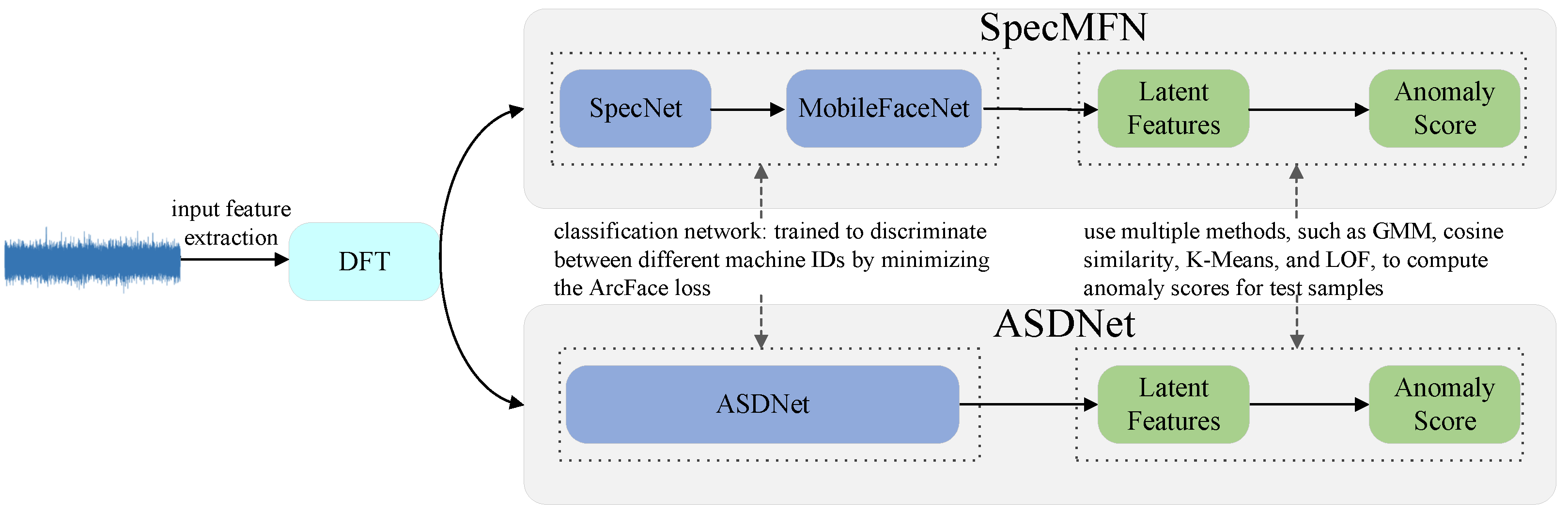
The overall framework of the proposed method is illustrated in Figure 1. This method utilizes spectral features as input and integrates two independent detection frameworks: SpecMFN and ASDNet. SpecMFN combines SpecNet and MobileFaceNet to achieve high detection accuracy, particularly excelling in pAUC, making it suitable for high-sensitivity and robust anomaly detection tasks. On the other hand, ASDNet is a lightweight network specifically optimized for resource-constrained environments, such as embedded systems or real-time detection applications. It significantly reduces computational complexity while maintaining strong detection performance, providing an efficient solution for scenarios with limited resources. During the training phase, Mixup [38] is employed as a data augmentation technique to mitigate overfitting and enhance the robustness of the models. Both frameworks ultimately utilize multiple methods for anomaly scoring, including cosine similarity, GMM, K-Means, and LOF. The subsequent sections provide a detailed explanation of input feature extraction, the design of classification networks, and the methods used for calculating anomaly scores.

2.1. Mixup

The utilization of the Mixup strategy for data augmentation has proven to be an effective approach for mitigating model overfitting and enhancing classification accuracy [19]. When combined with the ArcFace loss function [15], it significantly improves intra-class compactness while increasing inter-class separability.

In contrast to conventional data augmentation techniques, Mixup combines two independent data samples and their respective class labels within the same batch. The procedure can be described as follows:

$$x_{ij}=\lambda x_i+(1-\lambda )x_j$$

(1)

$$y_{ij}=\lambda y_i+(1-\lambda )y_j$$

(2)

where $i\in \{1,\dots ,B\}$ and $j\in \mathrm{Shuffle}\{1,\dots ,B\}$ represent the indices of data x within a batch of size B. The mixing weight $\lambda \sim Beta(\alpha ,\alpha )$ is sampled from a Beta distribution with $\alpha =0.5$, ensuring that the generated input is biased toward either 0 or 1.

2.2. Input Feature

In self-supervised ASD systems, Log-Mel features are used in many studies, such as [13,14,15,25,29,30,39]. The extraction of Log-Mel spectrograms involves three key stages: Short-Time Fourier Transform (STFT) [40], Mel filter banks, and logarithmic compression.

The frequency and time resolutions of the STFT are given by the following:

$$\Delta f={\displaystyle \frac{f_s}{N}},\Delta t={\displaystyle \frac{N}{f_s}},$$

(3)

where $f_s$ is the sampling rate, and N is the window length.

The formulas above demonstrate that there is a trade-off between frequency and time resolution: larger window sizes improve frequency resolution but reduce time resolution, thereby limiting the ability to effectively capture transient low-frequency components. In contrast, spectral features provide higher frequency resolution and are more effective in capturing both high-frequency and low-frequency components. The non-uniform filter design of Log-Mel spectrograms reduces sensitivity to high-frequency information, while the windowing used in STFT limits the representation of low-frequency components. Spectral features, with their fine-grained frequency representation, offer a more comprehensive reflection of the spectral structure of sound signals. As a single input feature, spectral features avoid the redundancies associated with multi-feature fusion and provide high-quality, discriminative input data, thereby enhancing anomaly detection performance.

Recognizing these advantages, researchers have shifted their focus toward processing methods that emphasize frequency domain information. Wilkinghoff [30] and Guan et al. [41], for instance, introduced temporal marginalization techniques to aggregate temporal information in time–frequency representations, thereby prioritizing frequency feature extraction. By discarding temporal dynamics, their approach maximized the potential of spectral features, thereby highlighting their value in anomaly detection tasks.

Inspired by this, our study directly focuses on frequency domain information by employing spectral features as the primary input, enabling more effective capture of critical frequency components. Specifically, we apply the Discrete Fourier Transform (DFT) to convert audio signals into frequency domain representations. For an audio signal $x\left(n\right)$ of length L, the DFT is computed as follows:

$$X\left(k\right)=\sum _{n=0}^{L-1}x\left(n\right)·e^{-j2\pi kn/L},k=0,1,\dots ,L-1.$$

(4)

By leveraging spectral features, our proposed approach captures anomalous patterns more effectively, thereby significantly enhancing detection performance while maintaining computational efficiency.

2.3. Network

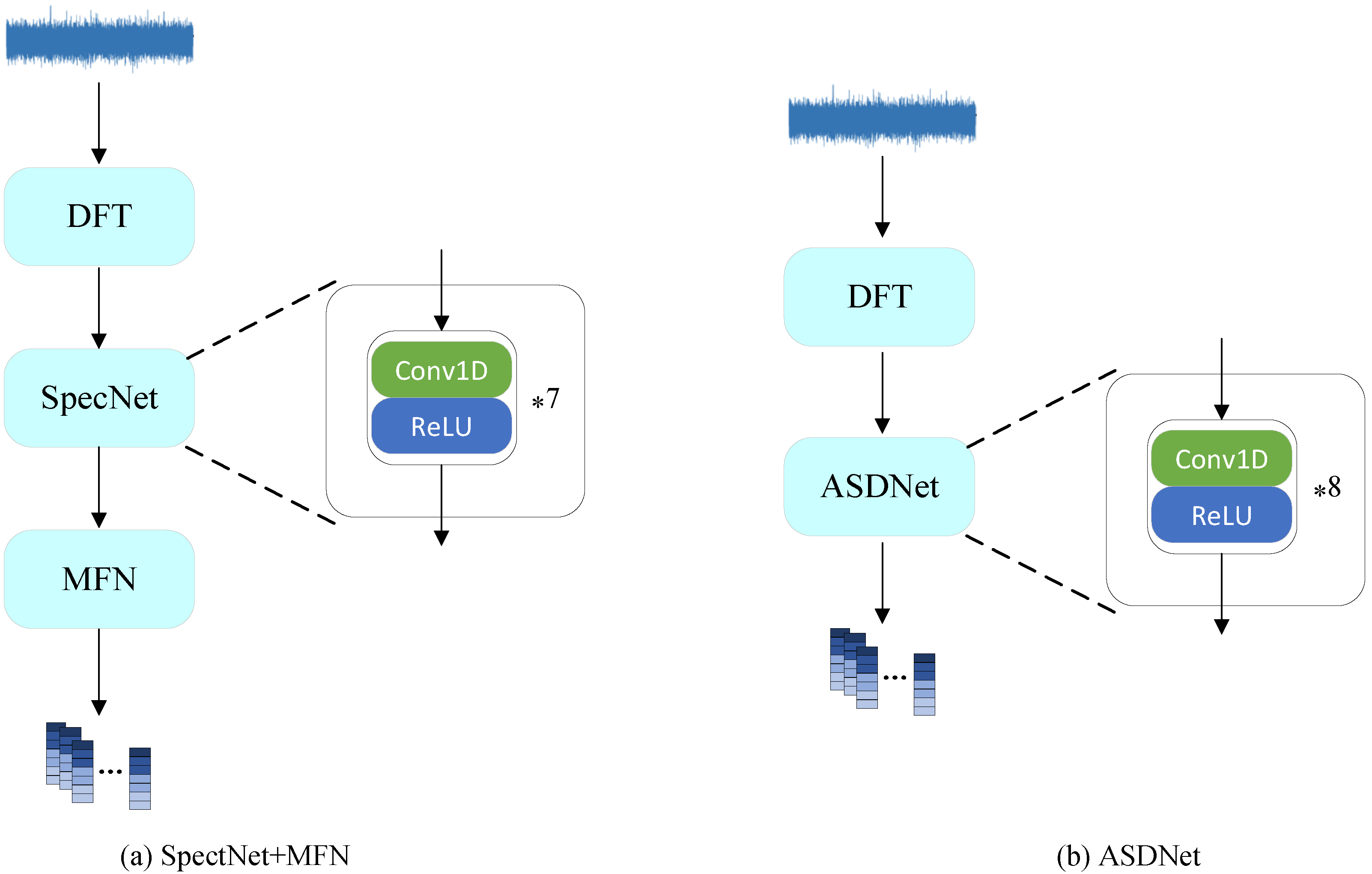
Classification neural networks play a critical role in self-supervised ASD detection by extracting latent features and utilizing classification learning to effectively distinguish between different sound patterns. Self-supervised ASD methods based on classification networks have been demonstrated to outperform traditional approaches, especially in handling complex anomalous patterns [7]. In this study, we propose two classification network architectures to meet the requirements of resource-constrained environments and high-sensitivity detection tasks: the lightweight ASDNet, and SpecMFN, which combines SpecNet and MobileFaceNet, as illustrated in Figure 2.

ASDNet is optimized for resource-constrained environments, with the goal of reducing model parameters and computational overhead while maintaining robust detection performance, making it well suited for deployment on edge devices. In contrast, SpecMFN integrates a spectral feature processing network (SpecNet) with an efficient classification network (MobileFaceNet), thereby enhancing its ability to detect complex anomalous patterns. Notably, performance evaluations indicate that SpecMFN achieves a higher partial area under the curve (pAUC) than ASDNet, highlighting its superior ability to capture anomalous patterns in regions with low false positive rates (FPR). This makes SpecMFN particularly suitable for applications that require high detection precision. Together, these two architectures provide flexible and efficient solutions tailored to diverse application needs.

2.3.1. ASDnet

ASDNet is a lightweight neural network specifically designed for resource-constrained environments. It processes spectral features to extract deep latent representations. The network architecture, as detailed in

Table 1. ASDNet architecture configuration.

Layer	Operator	Channels	Kernel Size	Stride
1	Conv1D	128	9	6
2	Conv1D	128	7	5
3	Conv1D	128	5	3
4	Conv1D	128	5	3
5	Conv1D	128	3	2
6	Conv1D	128	3	2
7	Conv1D	128	3	2
8	Conv1D	128	3	2

, combines one-dimensional convolutions with ReLU activation functions to perform feature extraction and compression. To enhance computational efficiency, ASDNet utilizes larger convolution strides, thereby significantly reducing the number of parameters and computational overhead, while maintaining robust detection performance.

The ASDNet architecture consists of eight processing steps, each comprising a one-dimensional convolution operation followed by a ReLU activation function. The computation process for each step is described as follows:

$$f_{i,k}=\sigma \left(\sum _{j\in {\mathcal{R}}_i}{w}_{j,k}·x_j+b_k\right),$$

(5)

where $f_{i,k}$ represents the output of the k-th convolution kernel in the i-th layer, ${\mathcal{R}}_i$ denotes the receptive field of the neuron, $w_{j,k}$ is the weight coefficient of the convolution kernel, $b_k$ is the bias term, and $\sigma (·)$ is the ReLU activation function.

The extracted latent feature z can be computed using the classification network $f_{\mathrm{ASDNet}}(·)$, as follows:

$$z=f_{\mathrm{ASDNet}}(x;\theta ),$$

(6)

where $\theta$ represents the parameters of ASDNet.

During the training phase, both ASDNet and SpecMFN employ ArcFace Loss to optimize classification performance. ArcFace Loss introduces an angular margin, which enhances intra-class compactness and inter-class separability, thereby improving the model’s discriminative ability. The loss function is defined as follows:

$$L=-{\displaystyle \frac{1}{N}}\sum _{i=1}^{N}log{\displaystyle \frac{e^{s·(cos({\theta }_{y_i}+m))}}{e^{s·(cos({\theta }_{y_i}+m))}+{\sum }_{j\ne y_i}{e}^{s·cos\left({\theta }_j\right)}}},$$

(7)

where ${\theta }_{y_i}$ denotes the angle between the input feature and the corresponding class center, m is the angular margin, s is the scale parameter, and N is the batch size.

2.3.2. SpecMFN

SpecMFN integrates the frequency domain processing network SpecNet with the classification network MobileFaceNet, designed to enhance anomaly detection performance. SpecNet focuses on refining spectral features and extracting detailed latent representations. Its architecture, consisting of 1D convolutional layers and ReLU activation functions, is similar to ASDNet. However, SpecNet employs fewer layers and smaller convolutional strides compared to ASDNet, enabling finer-grained feature extraction tailored for high-precision tasks.

MobileFaceNet, used as the backend classification network, is specifically optimized for lightweight and efficient feature classification. By leveraging depthwise separable convolutions and a linear bottleneck structure, MobileFaceNet strikes an effective balance between computational efficiency and classification accuracy, making it well suited for deployment in resource-constrained environments.

To ensure a consistent evaluation framework, this study adopts the MobileFaceNet architecture from Liu et al. [13] to compare the performance of spectral features against Log-Mel features, facilitating a fair and reliable assessment.

2.4. Different Methods for Anomaly Score Calculation

In classification-based ASD systems, pseudo-labels are typically generated from machine attributes, and anomaly scores are computed using classification confidence. However, these methods have significant limitations. Pseudo-labels often only capture the superficial characteristics of normal data, while classification confidence is not well suited for detecting anomalies that are sparsely distributed or significantly deviate from normal patterns. As a result, these methods may fail to achieve the desired accuracy and robustness in anomaly detection.

To address these limitations, this study proposes calculating anomaly scores using multiple methods, including cosine similarity, K-Means, GMMs, and LOF. Each method provides a unique approach for anomaly evaluation: cosine similarity measures the difference in similarity between samples, K-Means identifies outliers by clustering data, GMMs detect anomalies based on probabilistic distribution characteristics, and LOF identifies anomalies through local density analysis. By employing these methods, this study offers a more comprehensive and nuanced framework for anomaly detection, compensating for the limitations of traditional classification-based approaches.

2.4.1. Cosine Similarity

Cosine similarity [37] is a metric used to measure the degree of similarity between two vectors in a multi-dimensional space. Unlike direct comparisons of vector magnitudes, cosine similarity evaluates the angle between two vectors to determine their directional alignment. Cosine similarity has been widely used in various audio processing tasks. For instance, in speech recognition [42], it measures the similarity between different speech signals; in speaker identification [20], it compares the similarity of speaker-specific features. Furthermore, in the domain of anomalous sound detection, Wu et al. [19] utilized cosine similarity to calculate anomaly scores. These applications collectively demonstrate the effectiveness and versatility of cosine similarity in speech and audio processing.

In anomaly detection, let the feature vector of the test sample be $z_i$, and the feature center of its corresponding normal class be ${\mu }_c$, which represents the mean feature vector of the normal data for that class. The cosine similarity between $z_i$ and ${\mu }_c$ is computed as follows:

$$\mathrm{Cosine}\mathrm{Similarity}=cos(z_i,{\mu }_c)={\displaystyle \frac{z_i·{\mu }_c}{\parallel z_i\parallel \parallel {\mu }_c\parallel }}$$

(8)

After calculating the similarity, the anomaly score $A_{\cos }$ is derived as follows:

$$A_{\cos }=-ln\left(|cos(z_i,{\mu }_c)|\right)$$

(9)

$A_{\cos }$ is the anomaly score, with smaller scores indicating more typical data points and larger scores indicating higher likelihood of being an anomaly.

2.4.2. K-Means

K-Means [34] is a widely used unsupervised learning algorithm [43]. It partitions a dataset into k non-overlapping clusters, ensuring that samples within the same cluster are highly similar, while samples in different clusters are distinctly different. Each cluster is represented by its centroid, which is computed as the geometric mean of the samples within the cluster. The similarity between data points and centroids is typically measured using Euclidean distance.

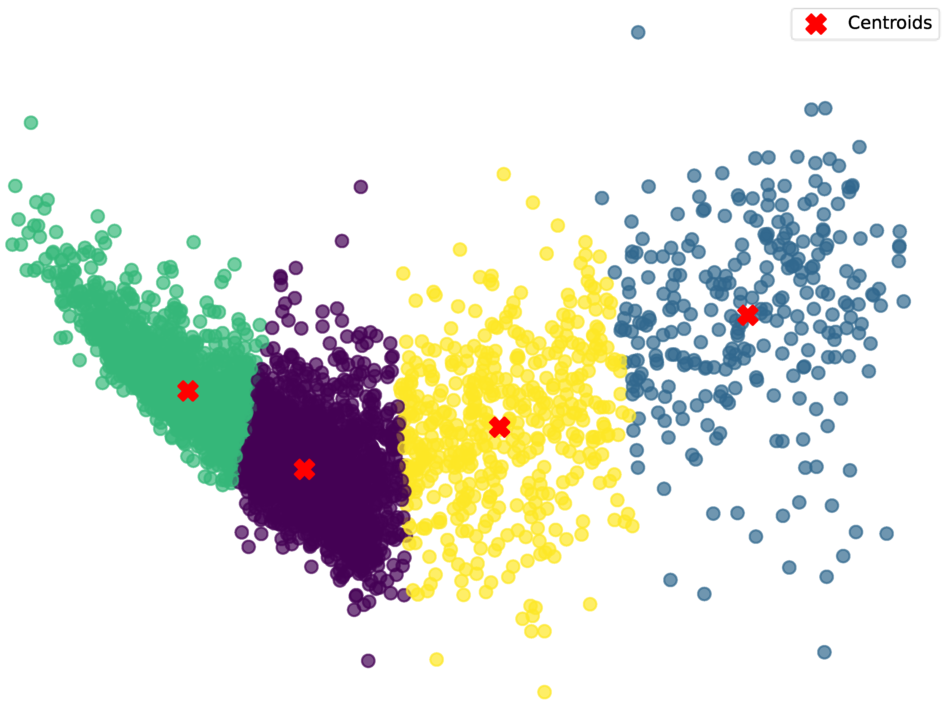
The process of calculating anomaly scores using K-Means consists of two main steps: first, performing K-Means clustering on the normal latent features of a specific class to obtain the cluster centers; second, calculating the distance between the latent features of the test samples and the cluster centers to determine the anomaly scores. The method for obtaining the cluster centers is shown in Algorithm 1, and the visualization of the clustering results is presented in Figure 3.

For anomaly detection, the distance between the test sample and the cluster centers can also be measured using cosine similarity. Specifically, we calculate the anomaly score by measuring the cosine similarity between the feature vector $z_i$ of the test sample and the centroids ${\mu }_{c,j}$ of all clusters in its corresponding category c, computed as follows:

$$cos(z_i,{\mu }_{c,j})={\displaystyle \frac{z_i·{\mu }_{c,j}}{\parallel z_i\parallel \parallel {\mu }_{c,j}\parallel }}$$

(10)

Subsequently, the cluster with the highest cosine similarity to $z_i$ is identified as the closest cluster, and the calculation is given by the following:

$$\mathrm{best}\text{\_}\cos =\underset{j}{max}\left(|cos(z_i,{\mu }_{c,j})|\right)$$

(11)

Finally, the anomaly score is derived from the best similarity value $\mathrm{best}\text{\_}\mathrm{cs}$ using the following formula:

$$A_{K\_Means}=-ln\left(\mathrm{best}\text{\_}\cos \right)$$

(12)

Here, $A_{K\_Means}$ represents the anomaly score, and the higher the value, the more likely the data point is an anomaly.

Algorithm 1 K-Means algorithm

Input:     $\{z_1,z_2,z_3,\cdots ,z_n\}\in Z$: set of latent features extracted from the training data Z     $\{C_1,C_2,C_3,\cdots ,C_k\}\in C$: set of clusters C     $maxiter$: number of allowed maximum iterations Steps: 1:   Assign initial centers ${\mu }_1,{\mu }_2,{\mu }_3,\cdots ,{\mu }_k$ randomly 2:   repeat 3:         $C_1,C_2,\cdots ,C_k\leftarrow \varnothing$ 4:         for each $z\in Z$ do 5:               $i=arg{min}_{i=1,\cdots ,k}{\parallel z-{\mu }_i\parallel }^2$ 6:               $C_i\leftarrow C_i\cup \left\{z\right\}$ 7:         end for 8:         for $i=1,\cdots ,k$ do 9:               if $C_i\ne \varnothing$ then 10:                    ${\mu }_i={\displaystyle \frac{1}{|C_i|}}{\sum }_{z\in C_i}z$ 11:               end if 12:         end for 13:   until the cluster centers ${\mu }_1,{\mu }_2,{\mu }_3,\cdots ,{\mu }_k$ do not change or $maxiter$ is reached

2.4.3. Gaussian Mixture Models

GMMs [35] represent a probabilistic model commonly employed for clustering tasks. The model assumes that the dataset is generated by a mixture of several distinct Gaussian distributions (i.e., multivariate normal distributions). Each cluster is represented by a specific Gaussian distribution, and the entire dataset is assumed to be a random sample drawn from k Gaussian distributions. Each distribution is characterized by its mean vector ${\mu }_i$, covariance matrix ${\Sigma }_i$, and mixing weight ${\pi }_i$, where ${\pi }_i$ denotes the proportion of that distribution in the overall dataset. These parameters enable GMMs to flexibly model complex cluster shapes.

The probability density function (PDF) of a GMM is the weighted sum of its Gaussian components. The formula for the GMM PDF is given by the following:

$$p\left(z\right|Y)=\sum _{i=1}^k{\pi }_{i}N\left(z\right|{\mu }_i,{\Sigma }_i)$$

(13)

where $N\left(z\right|{\mu }_i,{\Sigma }_i)$ represents the multivariate normal distribution of the i-th Gaussian component, which gives the probability density of the data point z under that distribution. $Y=\{{\pi }_i,{\mu }_i,{\Sigma }_i|i=1,\cdots ,k\}$ denotes the parameters of all k distributions in the mixture. ${\pi }_i,{\mu }_i,{\Sigma }_i$ are the mixture coefficient, mean vector, and covariance matrix of the i-th Gaussian distribution in the GMM, respectively.

Unlike models based solely on distances, GMM incorporates both distance and directional information through the full covariance matrix, allowing it to model more complex decision boundaries.

To define the anomaly score, we calculate the negative log-likelihood probability based on the GMM model:

$$A_{GMM}=-ln\left(p\left(z\right|Y)\right)$$

(14)

Here, $A_{GMM}$ represents the anomaly score. A higher value indicates a greater likelihood that the data point is an anomaly.

2.4.4. Local Outlier Factor

The LOF [36] algorithm is a density-based anomaly detection method that identifies outliers by comparing the local density of a data point to that of its neighbors. Specifically, LOF evaluates whether a data point is an outlier by calculating the ratio of its local density to the local densities of its neighboring points. If a data point’s local density is significantly lower than the densities of its neighbors and the ratio falls below a certain threshold, the point is considered an outlier. The main advantage of LOF is its ability to detect anomalies in datasets with varying local density distributions, making it particularly effective for cases where the data exhibits local density variations.

The core idea of LOF is to assess the anomaly degree by computing the local reachability density (LRD) for each data point and its neighbors. For each data point p, its LOF value is the average ratio of the LRD of its neighbors to the LRD of the point p. The formula for calculating LOF is as follows:

$$LOF\left(p\right)={\displaystyle \frac{1}{|N_k\left(p\right)|}}\sum _{o\in N_k\left(p\right)}{\displaystyle \frac{LRD\left(o\right)}{LRD\left(p\right)}}$$

(15)

where $N_k\left(p\right)$ is the set of k-nearest neighbors of point p, and $LRD\left(p\right)$ is the local reachability density of point p.

In this study, for each newly identified data point, we compute its LOF value and use the negative of this value as the corresponding anomaly score. The anomaly score $A_{LOF}$ is given by the following:

$$A_{LOF}=-LOF\left(p\right)$$

(16)

A lower anomaly score indicates that the data point is more typical, whereas a higher score suggests a greater likelihood of it being an anomaly.

3. Experiment and Analysis

This section provides additional information about the experimental dataset, implementation details, evaluation methodologies, results, and analysis.

3.1. Datasets

The proposed method is evaluated using the development and additional training datasets from the DCASE 2020 Challenge Task 2 [7], which include parts of two datasets: ToyADMOS [44] and MIMII [45]. These datasets consist of recordings of both normal and anomalous operating sounds from six types of machines: ToyCar, ToyConveyor, Valve, Pump, Fan, and Slide. Except for ToyConveyor, which contains six machine IDs, the remaining datasets contain seven machine IDs each. Anomalous sounds were intentionally generated by deliberately damaging the target devices. Each recording is a 10 s audio clip that captures both the operational sound of the machine and the surrounding environmental noise. All signals have been downsampled to a sampling rate of 16 kHz.

3.2. Implementation Details

The proposed model is trained using 2-s audio segments as input. After classification with ArcFace, the data is divided into 41 classes based on machine IDs. The Adam optimizer is used for training with a learning rate of 0.0001, and learning rate decay is implemented using a cosine annealing strategy. The batch size is set to 64. The ArcFace loss function employs a margin parameter of 0.5 and a scale factor of 30. The model is trained for 300 epochs on a system equipped with an Intel Core i9-9960X CPU and an NVIDIA RTX 4090D GPU, utilizing CUDA 11.8 and PyTorch 2.0.1.

3.3. Evaluation Methodology

This study employs the area under the receiver operating characteristic (ROC) curve (AUC) and partial AUC (pAUC) as evaluation metrics. pAUC is a metric that calculates the area under a certain range of interest on the ROC curve, specifically calculated as the AUC over a low false-positive rate ranging from 0 to p. The definitions of AUC and pAUC are given by the following formulas:

$$AUC={\displaystyle \frac{1}{N_{-}{N}_{+}}}\sum _{i=1}^{N_{-}}\sum _{j=1}^{N_{+}}\mathcal{H}({\mathcal{A}}_{\theta }\left(x_j^{+}\right)-{\mathcal{A}}_{\theta }\left(x_i^{-}\right))$$

(17)

$$pAUC={\displaystyle \frac{1}{\lfloor p{N}_{-}\rfloor N_{+}}}\sum _{i=1}^{\lfloor p{N}_{-}\rfloor }\sum _{j=1}^{N_{+}}\mathcal{H}({\mathcal{A}}_{\theta }\left(x_j^{+}\right)-{\mathcal{A}}_{\theta }\left(x_i^{-}\right))$$

(18)

Here, the symbol $\lfloor ·\rfloor$ denotes floor function. Function $\mathcal{H}\left(x\right)$ returns 1 if x is greater than 0; otherwise, it returns 0. ${\left\{x_i^{-}\right\}}_{i=1}^{N-}$ and ${\left\{x_j^{+}\right\}}_{j=1}^{N+}$ represent the sorted normal and abnormal test samples, respectively, and their anomaly scores are arranged in descending order. Here, $N_{-}$ represents the number of normal test samples and $N_{+}$ represents the number of anomalous test samples.

The pAUC is used to evaluate model performance, particularly in improving the true positive rate (TPR) at low false positive rates (FPR). This is essential because if the ASD system consistently generates inaccurate alerts, it becomes unreliable, as in the fable of “the boy who cried wolf”, who lost his credibility. The value of p in this experiment is set to 0.1.

In this study, we evaluate model complexity using two metrics: Floating-Point Operations (FLOPs) and the number of parameters. FLOPs represent the number of floating-point operations required for a single inference, providing insight into the model’s computational complexity and inference efficiency. The number of parameters refers to the total count of trainable parameters in the model, reflecting its storage capacity.

3.4. Comparison of Different Input Features

In this section, we compare the performance and computational complexity of different input features (such as spectral features and Log-Mel spectral features) and classification networks. The relevant results are summarized in

Table 2. Performance comparison of different input features and classification networks in terms of average AUC(%) and pAUC(%). Boldface denotes the best results.

Machine Type	LogMel-MFN		SpecMFN		ASDNet
	AUC	pAUC	AUC	pAUC	AUC	pAUC
Fan	92.30	84.06	99.39	98.15	98.63	95.17
Pump	92.20	84.30	96.72	91.76	94.86	89.04
Valve	99.02	95.01	96.73	86.76	97.26	88.87
Slider	99.17	96.37	99.78	98.82	99.56	97.83
ToyCar	94.41	84.92	97.06	90.14	96.80	89.15
ToyConveyor	71.66	61.92	76.51	66.00	79.41	63.04
Total	91.46	84.43	94.36	88.60	94.42	87.18

and

Table 3. Complexity comparison of different input and classification networks in terms of FLOPs and the number of parameters.

Network	Flops	# Params
LogMel-MFN	139.9 M	0.87 M
SpecMFN	184.2 M	1.05 M
ASDNet	85.4 M	0.51 M

, with anomaly scores calculated using the K-Means method.

In terms of performance across individual machine types, as shown in Table 2, SpecMFN demonstrates strong performance across several device types, particularly Fan, Pump, Slider, and ToyCar, where it achieves AUC and pAUC scores of 99.39% and 98.15%, 96.72% and 91.76%, 99.78% and 98.82%, and 97.06% and 90.14%, respectively. These results underscore SpecMFN’s strong ability to extract deep features and detect anomalies across various machines. In contrast, LogMel-MFN performs best on the Valve device, with AUC and pAUC scores of 99.02% and 95.01%. While ASDNet performs slightly worse on Valve than LogMel-MFN, it outperforms LogMel-MFN on most other devices, indicating a more balanced overall performance. Notably, compared to SpecMFN, ASDNet produces similar results across most devices and even surpasses SpecMFN on the Valve and ToyConveyor devices.

From an overall performance perspective, the difference between SpecMFN and ASDNet is minimal. SpecMFN achieves an AUC of 94.36% and a pAUC of 88.60%, while ASDNet scores 94.42% and 87.18%, respectively. Both models perform similarly across most devices, significantly outperforming LogMel-MFN (AUC of 91.46% and pAUC of 84.43%). This suggests that both SpecMFN and ASDNet are highly effective at capturing anomalous features in devices and exhibit strong robustness across a wide range of device types. Since both models use spectral features as input, the results further validate the effectiveness of spectral features for anomaly detection in this study. SpecMFN’s high average pAUC score underscores its superior detection precision and exceptional ability to accurately identify anomalous patterns across diverse devices, making it particularly well suited for high-sensitivity and robust anomaly detection tasks in demanding real-world applications.

In terms of computational complexity, as shown in Table 3, SpecMFN requires the most computation and has the highest parameter count among the models compared, which allows it to deliver superior detection performance, particularly excelling in pAUC for high-sensitivity applications. In contrast, ASDNet achieves 85.4 M FLOPs and 0.51 M parameters, which are only 46.4% and 48.6% of SpecMFN’s values, respectively, and 61.0% and 58.6% of LogMel-MFN’s values. While maintaining nearly the same accuracy as SpecMFN, ASDNet significantly reduces computational complexity, making it an efficient and practical choice for deployment in resource-constrained environments such as embedded devices or real-time applications.

3.5. Comparison of Different Method of Anomaly Score

Table 4. Performance comparison of different methods of anomaly scoring in terms of average AUC(%) and pAUC(%). Boldface denotes the best results.

Machine Type	PROB		COS		GMM		KMEANS		LOF
	AUC	pAUC	AUC	pAUC	AUC	pAUC	AUC	pAUC	AUC	pAUC
Fan	97.98	94.60	98.59	95.32	98.33	94.13	98.63	95.17	98.38	94.52
Pump	95.12	90.25	95.26	89.91	94.70	87.41	94.86	89.04	96.35	90.10
Valve	83.41	71.11	93.80	84.81	97.16	87.56	97.26	88.87	88.59	60.99
Slider	99.36	97.62	99.57	98.05	99.79	98.94	99.56	97.83	99.77	98.83
ToyCar	86.87	81.29	94.56	85.89	97.18	89.76	96.80	89.15	96.33	89.97
ToyConveyor	69.05	56.60	78.87	63.21	78.31	60.64	79.41	63.04	81.06	66.20
Total	88.63	81.91	93.44	86.20	94.25	86.41	94.42	87.18	93.41	83.43

presents a comparative analysis of the performance of various anomaly scoring methods. The PROB method calculates anomaly scores based on the Softmax probability output, whereas other methods—namely COS, GMM, KMEANS, and LOF—utilize latent features extracted from a neural network to model data distributions. Since the PROB method relies on the Softmax output of the classifier, it reflects the confidence of a sample belonging to a pseudo-label category. Notably, when machine IDs are used as pseudo-labels, the classifier primarily focuses on distinguishing between different machines, rather than differentiating between normal and anomalous points. As a result, PROB performs suboptimally in certain anomaly distributions. For example, on the ToyConveyor type, PROB achieves an AUC of 69.05% and a pAUC of 56.60%, both of which are significantly lower than those of other methods, highlighting its limitations in handling specific machine types.

In contrast, the methods COS, GMM, KMEANS, and LOF model data distributions directly from the latent features extracted by the neural network, allowing them to capture anomaly patterns more effectively. These methods avoid reliance on pseudo-labels, offering greater flexibility and robustness in detecting anomalies. Specifically, KMEANS outperforms other methods on the Fan and Valve types, with AUC and pAUC scores of 98.63% and 95.17%, and 97.26% and 88.87%, respectively. This demonstrates KMEANS’ ability to accurately identify anomalies and its strong adaptability across different machine types. The GMM method excels on the Slider type, achieving an AUC of 99.79% and a pAUC of 98.94%. On the ToyCar type, GMM achieves the highest AUC of 97.18%, with a pAUC near optimal at 89.76%, further emphasizing its strength in these two types. The LOF method performs outstandingly on both the ToyConveyor and Pump types, achieving an AUC of 96.35% for the Pump type. For the ToyConveyor type, the AUC is 81.06% and the pAUC is 66.20%. The COS method demonstrates relatively balanced performance across a wide range of machine types, with results close to the best performance, especially on the Fan and Pump types.

In summary, KMEANS ranks highest among all methods, with an AUC of 94.42% and a pAUC of 87.18%, owing to its consistently excellent performance and adaptability across a variety of machine types. GMM ranks second, as it excels in detecting anomalies in the Slider and ToyCar types, although its overall performance is slightly lower than that of KMEANS. The COS method ranks third, offering balanced performance across all machine types. While LOF exhibits advantages for certain types, such as ToyConveyor and Pump, its overall performance is relatively lower, suggesting it is better suited as a supplementary method.

KMEANS demonstrates exceptional and stable performance across multiple machine types, making it a highly suitable method for anomaly detection in various practical applications. In particular, its strong performance across types such as Fan, Valve, and Slider positions it as an ideal candidate for deployment in a wide range of anomaly detection scenarios.

3.6. Comparison of Other Anomalous Sound Detection System

This section provides a comprehensive comparative analysis of single-feature and multi-feature methods in terms of both performance and computational complexity for ASD systems. A balanced K-Means method is used to calculate anomaly scores.

Table 5. Performance comparison between multi-feature and single-feature input methods. Boldface denotes the best results.

Methods	Fan	Pump	Slider	Valve	ToyCar	ToyConveyor	Average
	AUC/pAUC	AUC/pAUC	AUC/pAUC	AUC/pAUC	AUC/pAUC	AUC/pAUC	AUC/pAUC
Multi-feature input methods
STgram-MFN [13]	94.04/88.97	91.94/81.75	99.55/97.61	99.64/98.44	94.44/87.68	74.57/63.60	92.36/86.34
SW-Wavenet [14]	97.53/91.54	87.27/82.68	98.96/94.58	99.01/97.26	95.49/90.20	81.20/68.20	93.25/87.41
ASD-AFPA [23]	97.55/93.48	94.46/86.76	99.69/98.40	99.12/95.42	96.12/89.45	76.49/64.21	93.91/87.95
CLP-SCF [39]	96.98/93.23	94.97/87.39	99.57/97.73	99.89/99.51	95.85/90.19	75.21/62.79	93.75/88.48
LMS-MobileNetV3 [24]	91.86/85.64	91.30/83.27	97.56/95.64	95.31/90.23	92.08/88.27	84.57/75.83	92.14/86.48
Single-feature input methods
LogMel-MFN [13]	82.36/–	87.74/–	99.08/–	89.91/–	88.73/–	78.17/–	87.67/–
Spectrogram-WaveNet [14]	83.45/–	85.94/–	98.00/–	97.68/–	94.54/–	80.53/–	90.03/–
LogMel-MobileNetV3 [24]	82.28/71.31	84.91/73.28	93.62/87.58	88.32/79.32	87.81/80.36	84.42/75.21	86.89/77.84
SpecMFN	99.38/98.15	96.72/91.76	96.73/86.76	99.78/98.82	97.06/90.14	76.51/66.00	94.36/88.60
ASDNet	98.63/95.17	94.86/89.04	97.27/88.87	99.56/97.83	96.90/89.15	79.41/63.04	94.42/87.18

presents a detailed comparison of AUC and pAUC performance across various tasks, highlighting the significant improvements achieved by our proposed single-feature methods (ASDNet and SpecMFN), which are based on spectral features.

Table 6. Complexity comparison of different ASD systems in terms of FLOPs and the number of parameters.

Network	Flops	# Params.
Multi-feature input methods
STgram-MFN [13]	1.62 G	1.16 M
SW-WaveNet [14]	21.56 G	34.47 M
ASD-AFPA [23]	1.71 G	1.55 M
CLP-SCF [39]	1.62 G	1.19 M
LMS-MobileNetV3 [24]	417.36 M	1.80 M
Single-feature input methods
LogMel-MFN [13]	1.38 G	0.87 M
Spectrogram-WaveNet [14]	10.78 G	17.17 M
LogMel-MobileNetV3 [24]	411.59 M	1.79 M
SpecMFN	184.2 M	1.05 M
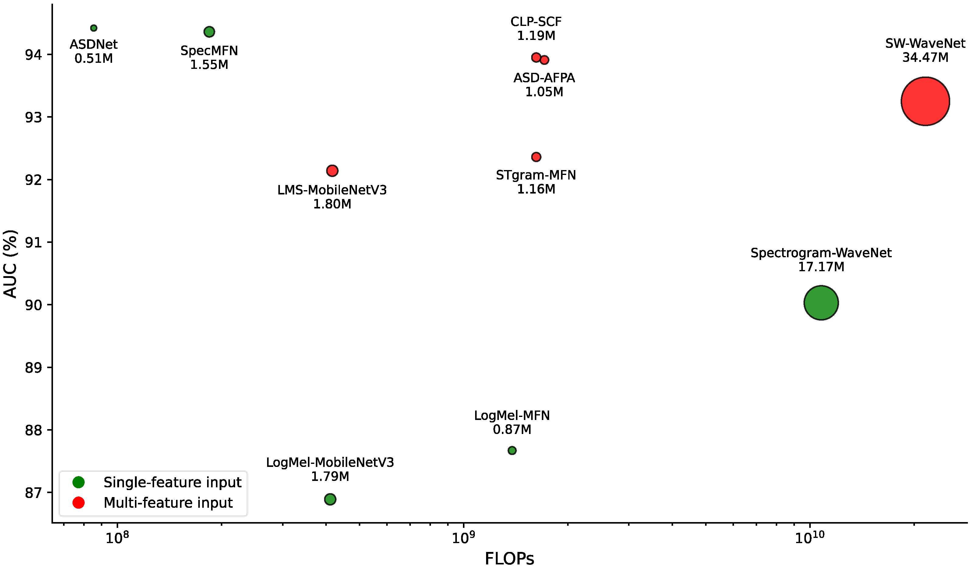
ASDNet	85.4 M	0.51 M

further analyzes the computational complexity of each method, emphasizing the superior hardware efficiency of the single-feature approaches. Additionally, the overall advantages of ASDNet and SpecMFN are visually illustrated in Figure 4: they are positioned at the top (indicating high AUC), to the left (indicating low FLOPs), and with smaller point sizes (indicating low parameter counts). These positions reflect an optimal balance between performance and hardware cost.

Table 5 summarizes the performance comparison between our methods and previous approaches, categorized into single-feature and multi-feature methods. The results indicate that the proposed single-feature methods (ASDNet and SpecMFN) outperform other single-feature methods across most tasks and evaluation metrics. For specific machine types, ASDNet and SpecMFN significantly outperform other single-feature methods in tasks such as Fan, Pump, Slider, Valve, and ToyCar. Notably, they even surpass multi-feature methods in tasks like Fan, Pump, and ToyCar. On Slider and Valve tasks, their performance is comparable to that of multi-feature methods, further validating their robustness and applicability across different tasks.

In terms of overall average metrics, ASDNet achieves an average AUC of 94.42% and pAUC of 87.18%, showing improvements of 6.75% and 4.39%, respectively, over LogMel-MFN [13] and Spectrogram-WaveNet [14] in AUC, and 9.34% and 7.15% in pAUC. SpecMFN achieves an average AUC of 94.36% and pAUC of 88.60%, with improvements of 6.69% and 4.33% in AUC, and 10.09% and 7.61% in pAUC, respectively. Notably, ASDNet achieves the highest AUC among all single-feature methods, while SpecMFN’s performance is comparable to the best multi-feature methods. For pAUC, SpecMFN outperforms all other methods. Both ASDNet and SpecMFN exhibit exceptional stability and generalization across multiple tasks.

Table 6 presents a comparison of the computational complexity of different methods. In general, multi-feature methods tend to have higher FLOPs and parameter counts compared to single-feature methods. For instance, SW-WaveNet [14] requires 21.56 G FLOPs and has 34.47 M parameters, making it the most computationally and memory-intensive model. In contrast, both ASDNet and SpecMFN are more efficient while maintaining strong performance. Specifically, ASDNet has 85.4 M FLOPs and 0.51 M parameters, achieving reductions of 93.81% in FLOPs and 41.38% in parameters relative to LogMel-MFN [13], and 99.21% in FLOPs and 97.09% in parameters compared to Spectrogram-WaveNet [14]. SpecMFN has 184.2 M FLOPs and 1.05 M parameters, which represents a reduction of 86.65% in FLOPs compared to LogMel-MFN [13], and reductions of 98.29% in FLOPs and 93.88% in parameters compared to Spectrogram-WaveNet [14].

The results demonstrate that ASDNet and SpecMFN achieve an optimal balance between performance and hardware efficiency, making them particularly well suited for embedded devices and mobile applications in resource-constrained environments. In contrast, while multi-feature methods offer superior performance for specific tasks, their significantly higher hardware costs restrict their applicability in low-resource scenarios. Methods with high FLOPs and parameter counts, such as SW-WaveNet, face substantial limitations in real-world applications. These observations highlight the effectiveness of our single-feature methods, which leverage spectral features and efficient model architectures to deliver substantial performance improvements while maintaining low computational costs.

Figure 4 highlights the advantages of single-feature methods in terms of both performance and computational complexity. ASDNet and SpecMFN stand out due to their top-left positions (high AUC and low FLOPs) and small point sizes (low parameter counts), indicating their ability to achieve high performance while significantly reducing hardware costs, making them particularly suitable for resource-constrained environments. In contrast, other single-feature methods, such as LogMel-MFN [13] and Spectrogram-WaveNet [14], exhibit higher FLOPs and parameter counts, which lead to noticeably lower performance. This suggests that improvements in feature extraction or model architecture design could further enhance their performance, making them more efficient for practical applications.

Meanwhile, multi-feature methods generally incur higher hardware costs. For instance, SW-WaveNet [14] has 21.56 G FLOPs and 34.47 M parameters. Although it delivers strong performance (AUC of 93.25%), its high computational complexity renders it less feasible for practical applications, particularly in resource-constrained environments. Among multi-feature methods, ASD-AFPA [23] and CLP-SCF [39] strike a more favorable balance between performance and complexity, with FLOPs of 1.71 G and 1.62 G, and parameter counts ranging from 1.19 M to 1.55 M. However, their complexity still exceeds that of single-feature methods by a significant margin. In contrast, LMS-MobileNetV3 [24], although having relatively low FLOPs (417.36 M), exhibits higher computational complexity compared to ASDNet’s 85.4 M and SpecMFN’s 184.2 M. Moreover, LMS-MobileNetV3 has a substantially larger number of parameters than both ASDNet and SpecMFN.

In summary, the results further emphasize the ideal balance between performance and complexity achieved by our single-feature methods (ASDNet and SpecMFN). These methods not only lead in AUC and pAUC but also exhibit extremely low FLOPs and parameter counts, making them particularly suitable for resource-constrained scenarios. Moreover, the findings confirm that spectral features, combined with efficient model designs, allow these methods to achieve optimal performance while avoiding the redundancy and high complexity typically associated with multi-feature methods. This makes them an efficient and robust solution for anomaly detection tasks.

4. Discussion

4.1. Configuration Selection of ASDNet Architecture

In this section, we evaluate the performance of ASDNet under different configurations of layers, channels, and kernel sizes. The choice of an eight-layer network, 128 channels, and specific kernel sizes was based on the balance of performance observed in the experiments. As shown in

Table 7. Evaluation of ASDNet performances for different configurations of layers, channels, and kernel sizes. Boldface denotes the best results.

Category	AUC	pAUC	Flops	# Params.
Different Configurations of Layers
7	91.99	84.27	85.12 M	0.49 M
8 (ASDNet)	94.42	87.18	85.4 M	0.51 M
9	94.10	87.21	85.7 M	0.56 M
10	93.83	86.98	85.79 M	0.59 M
Different Configurations of Channels
64	92.80	86.32	22.12 M	0.14 M
128 (ASDNet)	94.42	87.18	85.4 M	0.51 M
192	94.07	87.30	189.65 M	1.11 M
256	93.84	86.57	335.07 M	1.94 M
option A	93.99	87.17	28.62 M	0.69 M
option B	92.70	84.01	6.68 M	0.13 M
option C	94.12	87.77	307.77 M	1.23 M
Different Configurations of Kernel Sizes
5	93.04	85.37	125.46 M	0.57 M
7	94.38	87.05	232.52 M	0.8 M
ASDNet	94.42	87.18	85.4 M	0.51 M
option D	93.63	85.76	166.31 M	0.74 M
option E	93.63	86.76	243.55 M	0.74 M

For different configurations of channels, “64”, “128”, “192”, and “256” represent models with constant channels across all layers. “Option A” uses the configuration [32, 64, 128, 192, 256, 192, 128, 128], “Option B” has [32, 32, 32, 64, 64, 64, 128, 128], and “Option C” follows [256, 256, 192, 192, 160, 160, 128, 128]. For different configurations of kernel sizes, ‘5’ and ‘7’ represent models with fixed kernel sizes of 5 and 7, respectively. ‘Option D’ uses an increasing kernel size sequence [3, 3, 5, 5, 7, 7, 9, 9], while ‘Option E’ alternates between increasing and decreasing kernel sizes [3, 5, 7, 9, 9, 7, 5, 3].

, this configuration effectively balances computational complexity with high detection accuracy. Through comparison of various configurations, we identified this setup as the most optimal and selected it as the final implementation of ASDNet.

In evaluating different network depths, we test configurations with 7, 8, 9, and 10 layers. The experimental results show that the eight-layer network (ASDNet) achieves the best performance, with an AUC of 94.42% and a pAUC of 87.18%. The nine-layer configuration shows a slight improvement in pAUC (87.21%) but a minor decrease in AUC (94.10%). The 10-layer configuration exhibits further performance decmidrule with an AUC of 93.83% and a pAUC of 86.98%. The seven-layer configuration has the lowest performance, with an AUC of 91.99% and a pAUC of 84.27%, indicating that fewer layers may limit model expressiveness. Overall, while adding layers may improve performance in some cases, it does not guarantee substantial improvements and may increase computational complexity. Thus, the eight-layer configuration strikes an optimal balance between accuracy and computational efficiency, making it the final choice.

For channel number selection, we test four configurations: fixed channels (64, 128, 192, 256) and three configurations with varying channels (Option A, Option B, Option C). The results show that as the number of channels increased, the model’s performance significantly improved, particularly when increasing from 64 to 128 channels, resulting in notable improvements in both AUC and pAUC. However, further increases in channel numbers led to performance degradation. For example, with 192 channels, the AUC dropped to 94.07%, and with 256 channels, it further decreases to 93.84%, while the pAUC drops to 86.57%. Meanwhile, computational complexity increases significantly. Among the varying channel configurations, Option A (increasing-then-decreasing channels) provides a good balance between performance and complexity. Although Option C achieves a higher pAUC of 87.77%, its computational complexity increases significantly, with FLops at 307.77 M and parameters at 1.23 M, while Option B does not show a performance improvement. Based on these results, we ultimately select the configuration with 128 channels, as it offers high detection accuracy while effectively controlling computational complexity.

For kernel size selection, the results in Table 7 show that as the kernel size increases, both AUC and pAUC improve, but at the cost of increased computational cost and parameter count. Comparing different kernel configurations—including the decreasing configuration used in this study, Option D (increasing kernel size), and Option E (increasing-then-decreasing)—we find that the configuration selected for this study achieves the best performance in terms of AUC and pAUC, while also minimizing computational cost and parameter count. Therefore, we ultimately select this configuration.

4.2. Performance Evaluation of LOF with Different Distance Metrics

This study investigates the impact of distance metrics on the LOF algorithm for anomaly detection, evaluating the performance of six distance metrics: Euclidean, Manhattan, Chebyshev, Cosine, Canberra, and Bray–Curtis. As shown in Figure 5, Euclidean distance achieves the highest AUC (93.41%), followed closely by Manhattan and Chebyshev distances. While slight differences in AUC and pAUC are observed across the metrics, the overall results were remarkably consistent, with most metrics achieving AUC values around 93% and pAUC values around 83%. This consistency highlights the robustness of the LOF algorithm to different distance metrics, suggesting that, for this dataset, the choice of metric does not significantly impact detection performance. However, the relatively lower performance of the Canberra distance (AUC: 90.36%, pAUC: 81.74%) demonstrates that not all metrics are equally effective, underscoring the importance of tailoring the selection of distance metrics to the specific characteristics of the dataset.

Although Euclidean distance proves to be a robust and reliable choice in this study, future research should focus on exploring more flexible approaches. For instance, hybrid or adaptive distance metrics could combine the strengths of multiple metrics to better accommodate diverse datasets, while dimensionality reduction techniques may help address challenges posed by high-dimensional spaces. Furthermore, introducing more diverse and advanced distance metrics and evaluating their effectiveness across a broader range of datasets and anomaly detection tasks could provide deeper insights into their strengths and limitations. Such efforts would further enhance the adaptability and robustness of anomaly detection methods in various real-world scenarios.

5. Conclusions

This paper addresses the challenge of balancing improved detection accuracy with reduced computational complexity in Anomalous Sound Detection. To tackle this, we propose an efficient self-supervised ASD method that integrates spectral features, lightweight network architectures, and clustering-based scoring mechanisms. Specifically, we replace traditional Log-Mel features with spectral features, which offer higher-resolution frequency details that significantly enhance the input features and improve detection accuracy. Additionally, we design two network architectures: (1) SpecMFN, a highly efficient feature extraction network combining SpecNet and MobileFaceNet, suitable for scenarios demanding high detection sensitivity and precision, and (2) ASDNet, a lightweight network optimized for resource-constrained environments. ASDNet achieves a significant reduction in computational complexity by reducing both the depth of convolutional layers and the number of parameters, making it ideal for deployment in low-resource settings. Furthermore, we systematically compare various anomaly scoring mechanisms, demonstrating the superiority of clustering-based methods in capturing the distribution characteristics of anomalous patterns. In contrast to traditional classification confidence-based methods, clustering-based scoring utilizes complex decision boundaries to more accurately identify a broader range of anomalous patterns.

Experimental results underscore the significant advantages of ASDNet and SpecMFN in terms of both performance and computational complexity. ASDNet achieves average AUC and pAUC values of 94.42% and 87.18%, respectively, while SpecMFN reaches 94.36% and 88.60%. Compared to LogMel-MFN, ASDNet improves AUC and pAUC by 6.75% and 9.34%, respectively, while SpecMFN achieves corresponding improvements of 6.69% and 10.09%. In terms of computational complexity, ASDNet requires only 85.4 M FLOPs and 0.51 M parameters, whereas SpecMFN requires 184.2 M FLOPs and 1.05 M parameters. Compared to LogMel-MFN, which demands 1.38 G FLOPs and 0.87 M parameters, ASDNet reduces FLOPs by 93.81% and parameter count by 41.38%, while SpecMFN achieves an 86.65% reduction in FLOPs. These results demonstrate that the proposed methods not only deliver outstanding performance but also significantly reduce computational complexity, making them especially suitable for resource-constrained embedded devices and edge computing environments.

In practical applications, the choice of network architecture and anomaly scoring methods should be tailored to the specific requirements of the task and the operational environment. SpecMFN, with its higher pAUC values, is particularly well suited for applications that require high sensitivity and precision. For instance, in high-precision industrial equipment monitoring (such as the operation of precision machinery), SpecMFN effectively minimizes the potential damage caused by false positives, thereby enhancing fault detection accuracy and preventing errors or downtime due to false alarms. In contrast, ASDNet is a lightweight network optimized for resource-constrained environments, making it ideal for low-cost consumer electronics, such as smart home devices or wearables. ASDNet reduces computational load and improves real-time responsiveness while maintaining accurate detection of anomalous sounds.

Different anomaly scoring methods are more suitable for different scenarios. The K-Means clustering method performs well in general applications, with an average AUC of 94.42% and pAUC of 87.18%, making it reliable for routine industrial equipment fault detection. However, for more specialized applications, selecting the most appropriate anomaly scoring method is crucial. For example, in the case of sliding mechanical equipment, the GMM method outperforms others, achieving an AUC of 99.79% and a pAUC of 98.94%. In pump equipment monitoring (such as water or oil pumps), the LOF method delivers better results, with an AUC of 96.35% and a pAUC of 90.10%. In applications where false positives are especially critical, such as in power equipment or medical devices, deploying a combination of network architectures and anomaly scoring methods, along with a voting mechanism, can further reduce the likelihood of false alarms and ensure system stability and safety.

Future research will focus on three key areas. First, we aim to deploy ASDNet and SpecMFN on edge devices and develop real-time anomaly detection systems to assess their performance and stability in industrial environments. Second, we will investigate novel combinations of input features and lightweight network architectures to address diverse industrial needs and drive the broader adoption of ASD technology. Finally, while KMeans, GMM, and LOF are foundational clustering algorithms, their performance in Anomalous Sound Detection tasks may not be optimal. More advanced methods, such as federated heuristic optimization based on fuzzy clustering or fixed-centered KMeans, could potentially offer improved performance. Exploring these alternatives will be part of our future work.