
Development of a Multidimensional Analysis and Integrated Visualization Method for Maritime Traffic Behaviors Using DBSCAN-Based Dynamic Clustering


Abstract
1. Introduction
2. Related Work
3. Materials and Methods
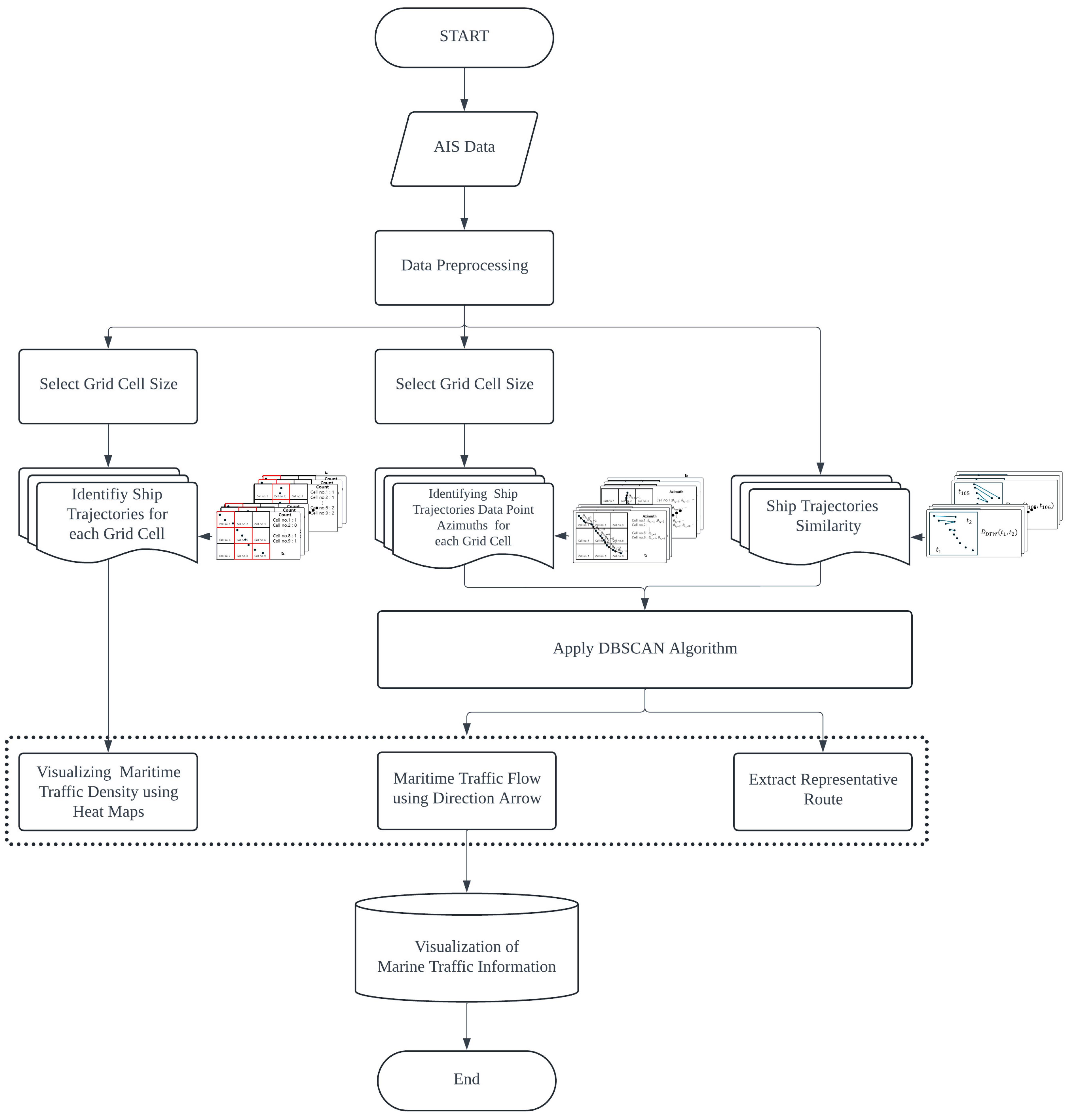
3.1. Process Flow
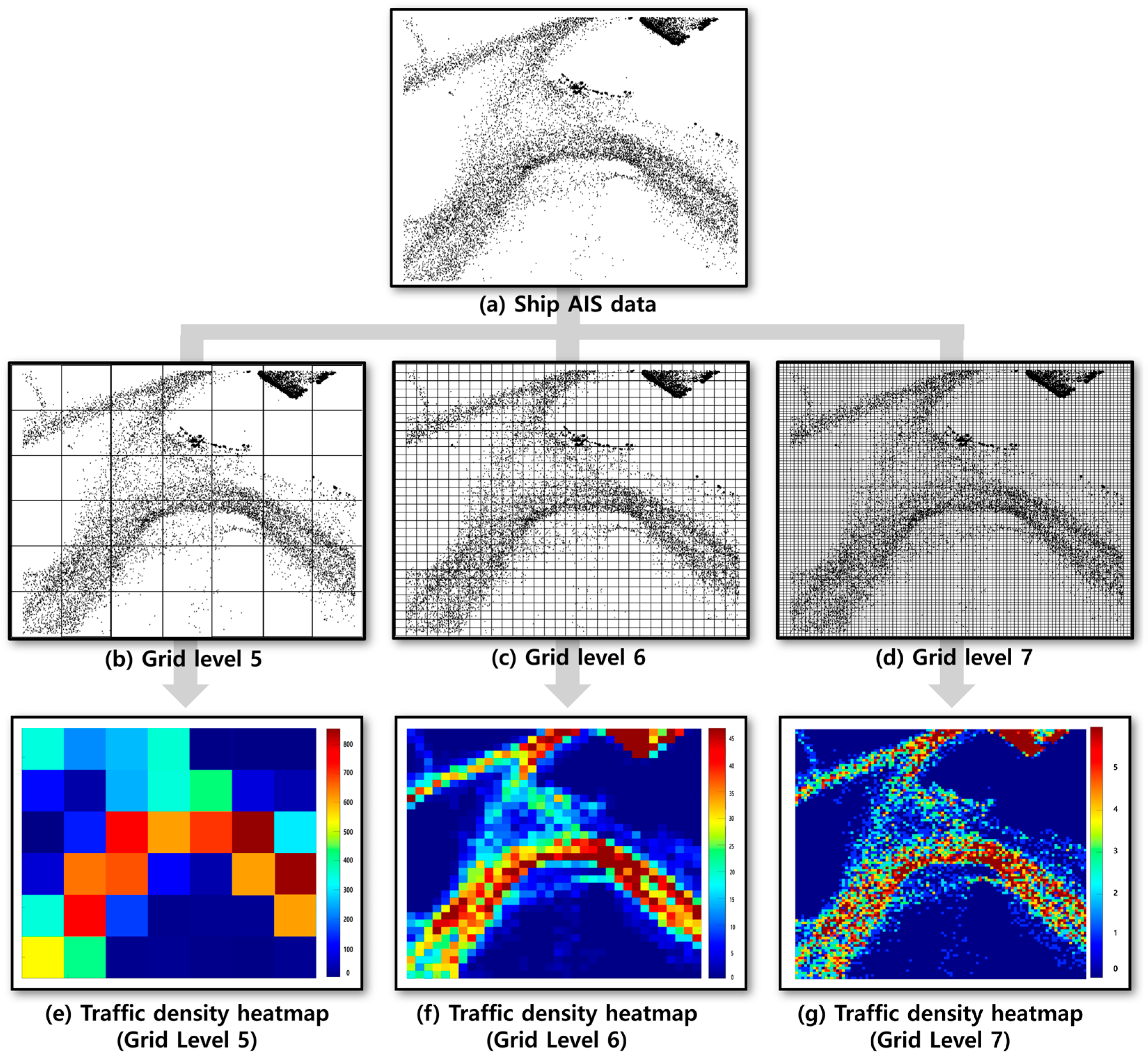
3.2. Traffic Density
3.2.1. Grid Cell Map
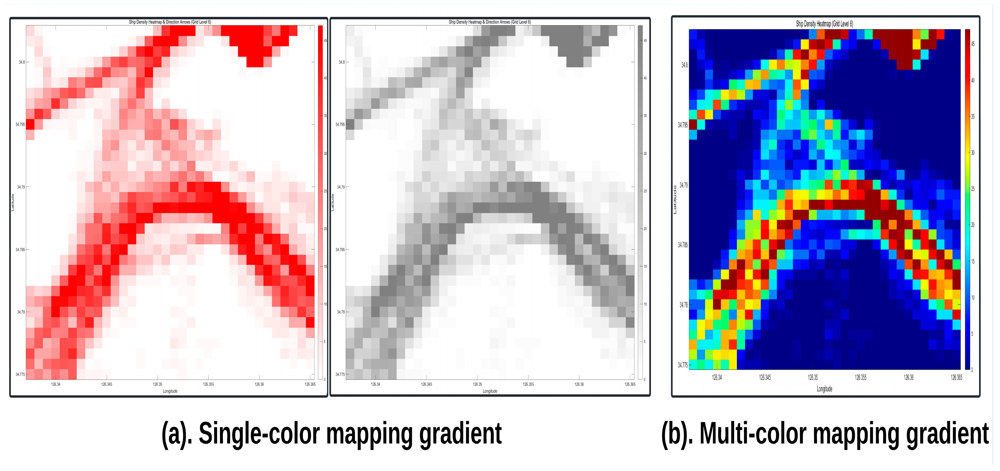
3.2.2. Visualization Process of Traffic Density
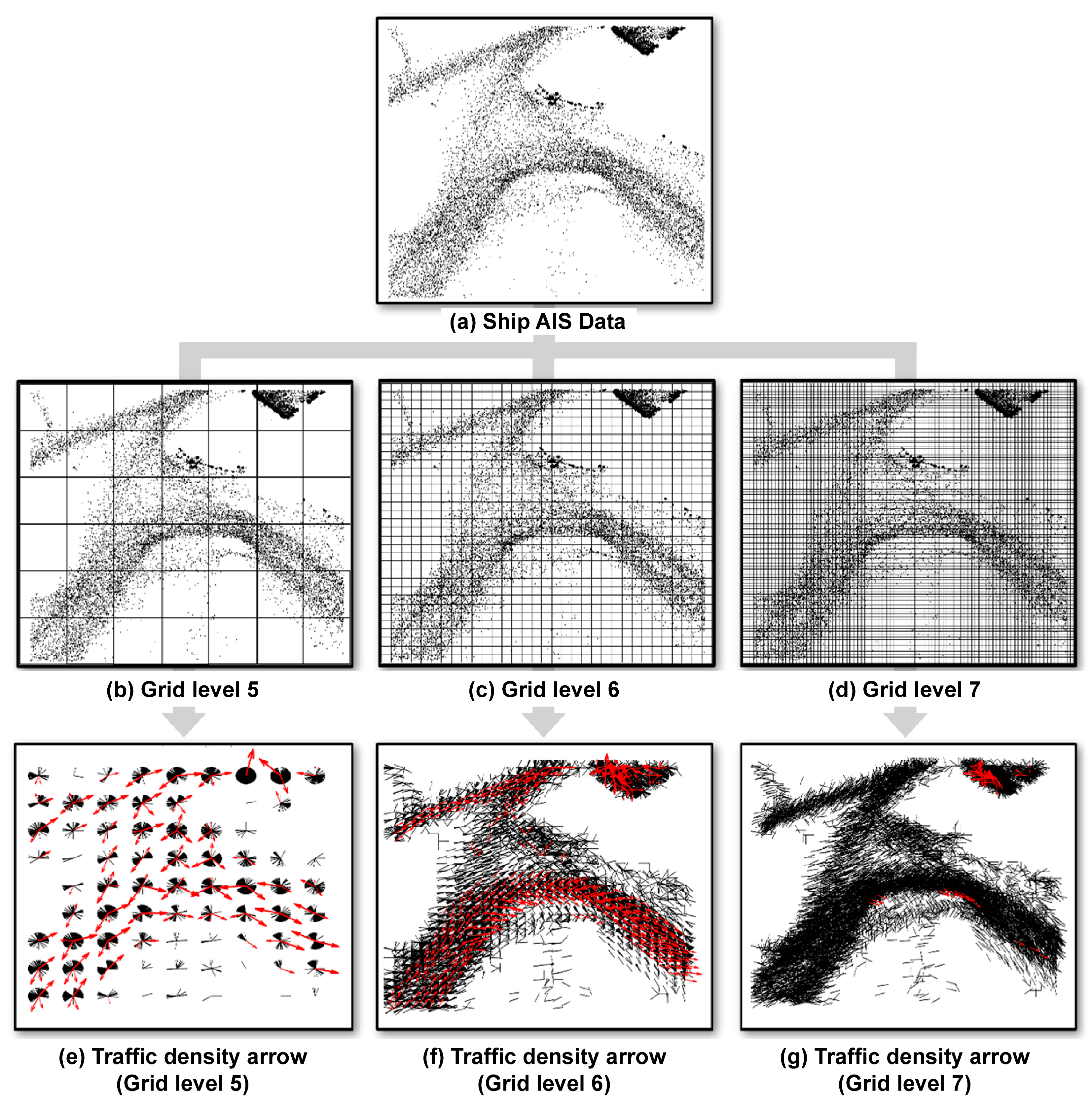
3.3. Traffic Direction
3.3.1. DBSCAN Algorithm
3.3.2. Azimuth Calculation
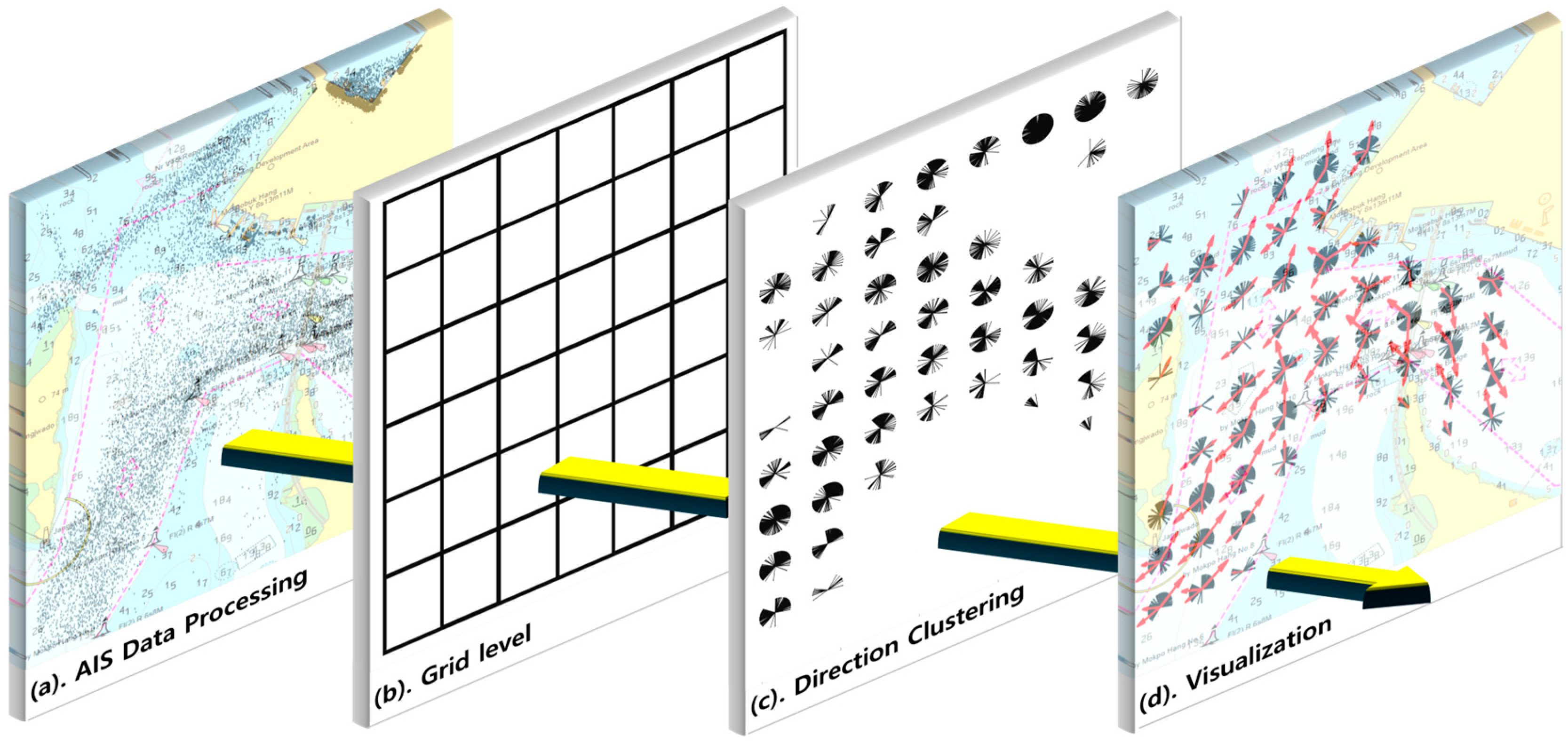
3.3.3. Visualization Process of Traffic Direction
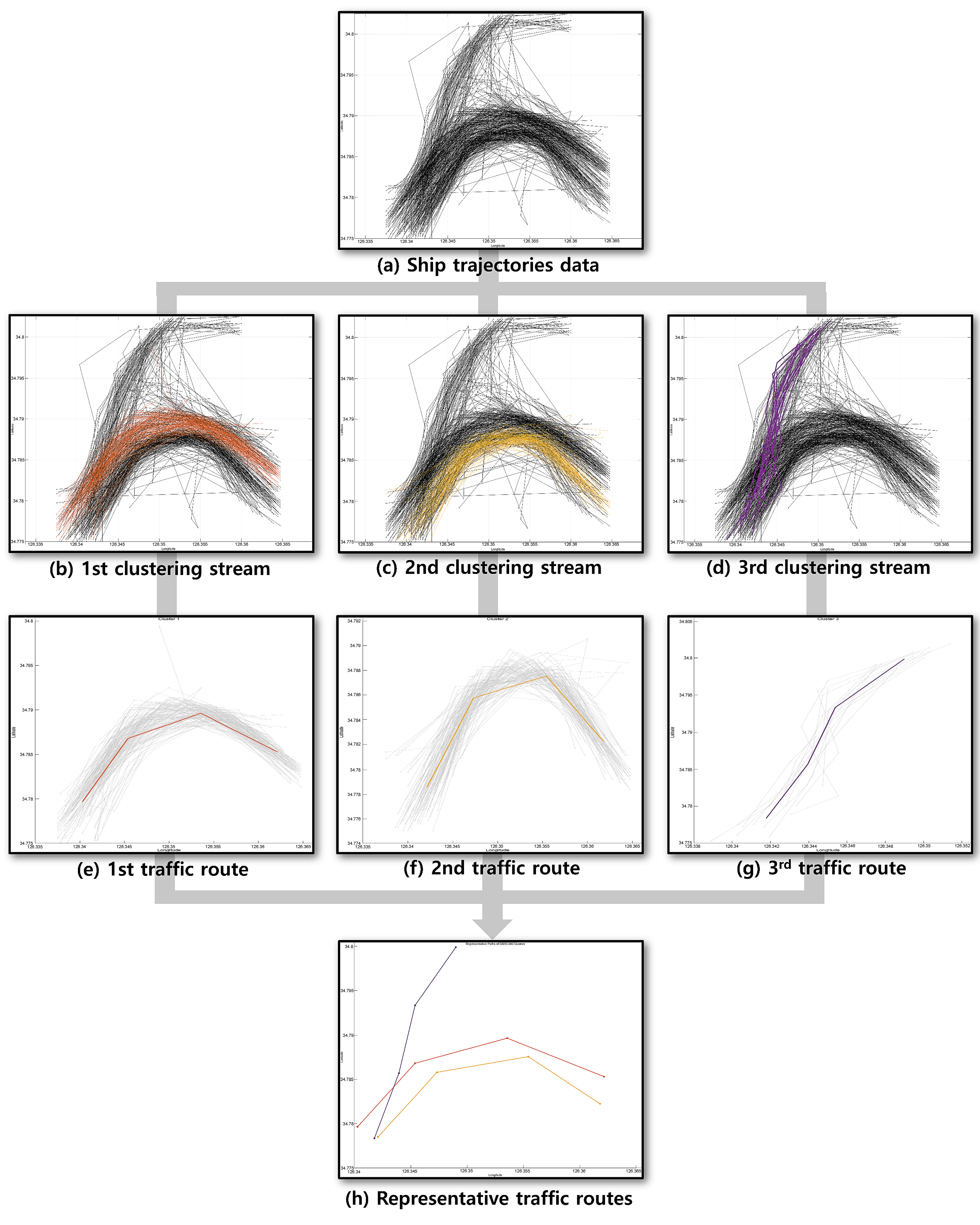
3.4. Traffic Stream
3.4.1. Trajectory Data Refinement
3.4.2. Measuring Similarity Between Ship Trajectories
3.4.3. Multidimensional Scaling
3.4.4. Extracting Representative Routes
3.4.5. Visualization Process of Traffic Stream
4. Application
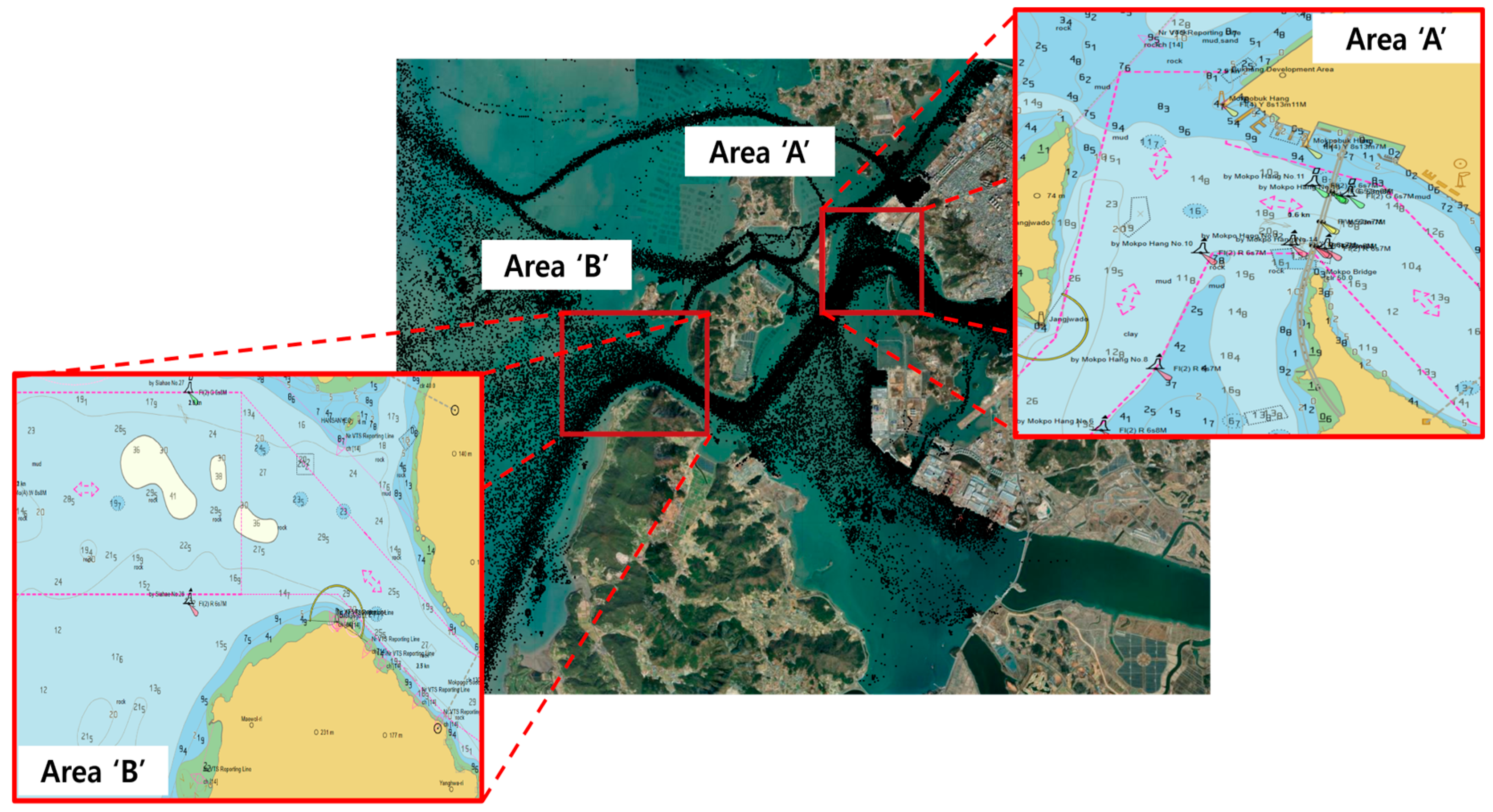
4.1. Study Area
4.2. Visualization of Traffic Density
4.3. Visualization of Traffic Direction
4.4. Visualization of Traffic Stream
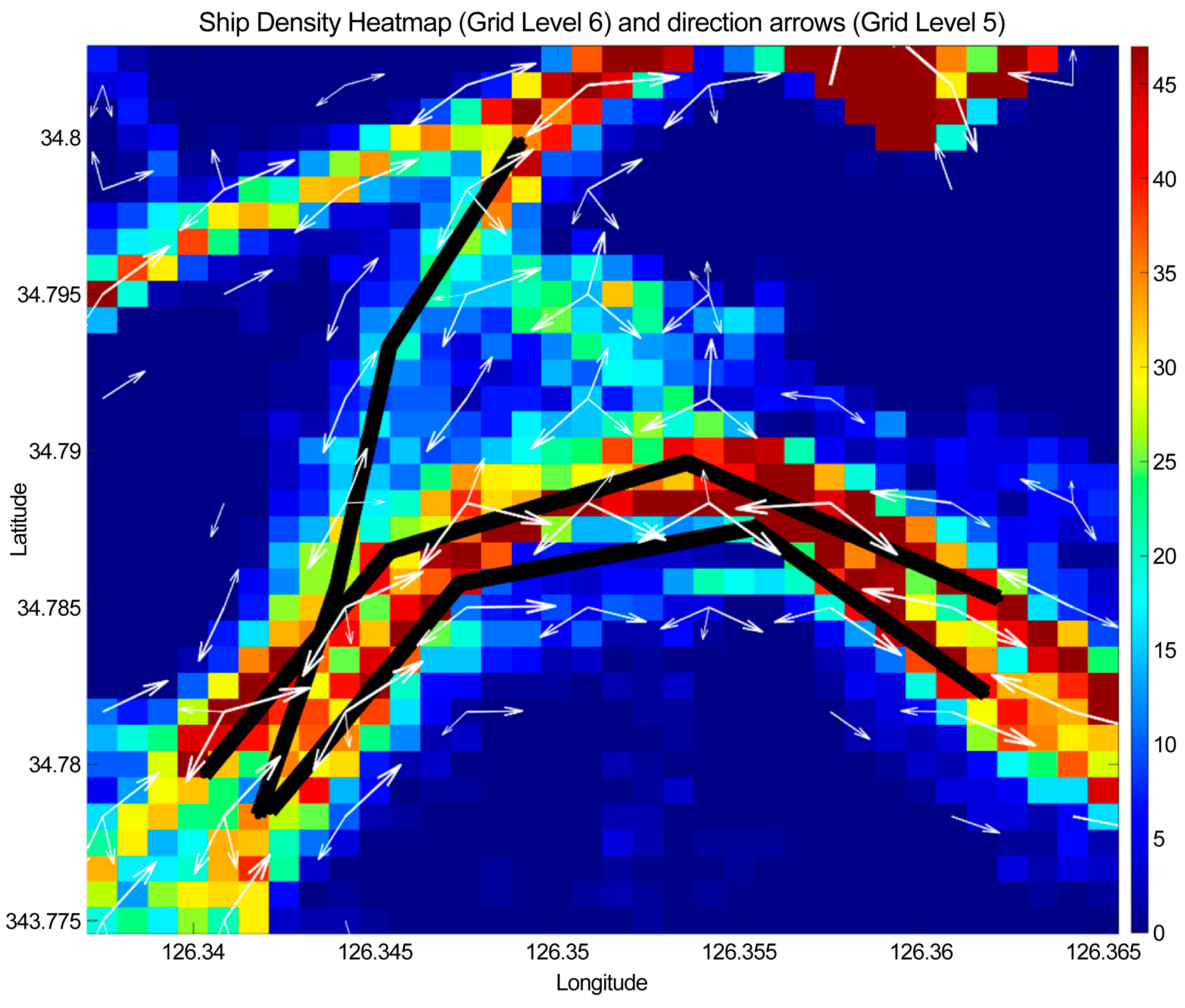
4.5. Visualization of Traffic Behaviors in Simulation Area “A”
4.6. Visualization of Traffic Behaviors in Simulation Area “B”
5. Conclusions
Author Contributions
Funding
Institutional Review Board Statement
Informed Consent Statement
Data Availability Statement
Acknowledgments
Conflicts of Interest
References
- Mazzarella, F.; Vespe, M.; Damalas, D.; Osio, G. Discovering vessel activities at sea using AIS data: Mapping of fishing footprints. In Proceedings of the 17th International Conference on Information Fusion (Fusion), Salamanca, Spain, 7–10 July 2014; pp. 1–7. [Google Scholar]
- Endsley, M.R. Design and evaluation for situation awareness enhancement. In Proceedings of the Human Factors Society 34th Annual Meeting, Santa Monica, CA, USA, 24–28 October 1988; Human Factors Society: Washington, DC, USA, 1988; Volume 32, pp. 97–101. [Google Scholar] [CrossRef]
- Sandhåland, H.; Oltedal, H.; Eid, J. Situation awareness in bridge operations—A study of collisions between attendant vessels and offshore facilities in the North Sea. Saf. Sci. 2015, 79, 277–285. [Google Scholar] [CrossRef]
- Cordon, J.R.; Mestre, J.M.; Walliser, J. Human factors in seafaring: The role of situation awareness. Saf. Sci. 2017, 93, 256–265. [Google Scholar] [CrossRef]
- International Maritime Organization. Strategy for the development and implementation of e-Navigation. In Med. Sci. 85/26/Add.1; IMO: London, UK, 2008; ANNEX 20. [Google Scholar]
- Ward, R.; Alexander, L.; Greenslade, B.; Pharaoh, A. IHO S-100: The new hydrographic geospatial standard for marine data and information. In Proceedings of the Canadian Hydrographic Conference and National Surveyors Conference, Victoria, BC, Canada, 4–8 May 2008. [Google Scholar]
- Scheepens, R.; Willems, N.; van de Wetering, H.; Andrienko, G.; Andrienko, N.; van Wijk, J.J. Composite density maps for multivariate trajectories. IEEE Trans. Vis. Comput. Graph. 2011, 17, 2518–2527. [Google Scholar] [CrossRef] [PubMed]
- International Hydrographic Organization (IHO). IHO Publication C-13. Manual on Hydrography; IHO: Monaco, 2005. [Google Scholar]
- International Maritime Hydrographic (IMO). IMO Ship’s Routeing Ed; IMO: London, UK, 2019. [Google Scholar]
- International Hydrographic Organization (IHO). IHO Transfer Standard for Digital Hydrographic Data, 3.1 ed.; IHO: Monaco, 2000. [Google Scholar]
- Zhang, M.; Zhang, D.; Fu, S.; Kujala, P.; Hirdaris, S. A predictive analytics method for maritime traffic flow complexity estimation in inland waterways. Reliab. Eng. Syst. Saf. 2022, 220, 108317. [Google Scholar] [CrossRef]
- Xin, X.; Liu, K.; Loughney, S.; Wang, J.; Yang, Z. Maritime traffic clustering to capture high-risk multi-ship encounters in complex waters. Reliab. Eng. Syst. Saf. 2023, 230, 108936. [Google Scholar] [CrossRef]
- Wu, X.; Rahman, A.; Zaloom, V.A. Study of travel behavior of vessels in narrow waterways using AIS data—A case study in Sabine-Neches waterways. Ocean Eng. 2018, 147, 399–413. [Google Scholar] [CrossRef]
- Dinis, D.; Teixeira, A.P.; Guedes Soares, C. Probabilistic approach for characterising the static risk of ships using Bayesian networks. Reliab. Eng. Syst. Saf. 2023, 203, 107073. [Google Scholar] [CrossRef]
- Xin, X.; Liu, K.; Loughney, S.; Wang, J.; Li, H.; Ekere, N. Multi-scale collision risk estimation for maritime traffic in complex port waters. Reliab. Eng. Syst. Saf. 2023, 240, 109554. [Google Scholar] [CrossRef]
- Rong, H.; Teixeira, A.P.; Guedes Soares, C. Maritime traffic probabilistic prediction based on ship motion pattern extraction. Reliab. Eng. Syst. Saf. 2022, 217, 108061. [Google Scholar] [CrossRef]
- Gil, M.; Koziol, P.; Wrobel, K.; Montewka, J. Know your safety indicator-A determination of merchant vessels bow crossing range based on big data analytics. Reliab. Eng. Syst. Saf. 2022, 220, 108311. [Google Scholar] [CrossRef]
- Fiorini, M.; Capata, A.; Bloisi, D.D. AIS data visualization for maritime spatial planning (MSP). Int. J. e-Navig. Marit. Econ. 2016, 5, 45–60. [Google Scholar] [CrossRef]
- Maragoudakis, M. Data analysis, simulation and visualization for environmentally safe maritime data. Algorithms 2019, 12, 27. [Google Scholar] [CrossRef]
- Shelmerdine, R.L. Teasing out the detail: How our understanding of marine AIS data can better inform industries, developments, and planning. Mar. Policy 2015, 54, 17–25. [Google Scholar] [CrossRef]
- Greidanus, H.; Alvarez, M.; Eriksen, T.; Gammieri, V. Completeness and accuracy of a wide area maritime situational picture based on automatic ship reporting systems. J. Navig. 2016, 69, 156–168. [Google Scholar] [CrossRef]
- Yoo, S.L. Near-miss density map for safe navigation of ships. Ocean Eng. 2018, 163, 15–21. [Google Scholar] [CrossRef]
- Wu, L.; Xu, Y.J.; Wang, Q.; Wang, F.; Xu, Z. Mapping global shipping density from AIS data. J. Navig. 2017, 70, 67–81. [Google Scholar] [CrossRef]
- Scheepens, R.; Hurter, C.; Van De Wetering, H.; Van Wijk, J.J. Visualization, selection, and analysis of traffic flows. IEEE Trans. Vis. Comput. Graph. 2016, 22, 379–388. [Google Scholar] [CrossRef]
- Seo, M.H.; Kim, G.U. Ship location information service using Automatic Identification System (AIS) and XML. Korea Inst. Inf. Commun. Eng. 2011, 15, 2590–2598. [Google Scholar] [CrossRef]
- Blu, T.; Thevenaz, P.; Unser, M. Linear interpolation revitalized. IEEE Trans. Image Process. 2004, 13, 710–719. [Google Scholar] [CrossRef]
- Kim, Y.J.; Lee, J.S.; Pititto, A.; Falco, L.; Lee, M.S.; Yoon, K.K.; Cho, I.S. Maritime traffic evaluation using spatial-temporal density analysis based on big AIS data. Appl. Sci. 2022, 12, 11246. [Google Scholar] [CrossRef]
- Akim, R.; Mustaffa, M.; Ahmad, S. Prediction of marine traffic density using different time series model from AIS data of Port Llang and Straits of Malacca. Trans. Marit. Sci. 2020, 9, 217–223. [Google Scholar] [CrossRef]
- Alexandros, T.K.; Giannis, S.; Vodas, M.; Zissis, D. Navigating dense waters toolbox creating marit density maps. In Proceedings of the SETN ’22: Proceedings of the 12th Hellenic Conference on Artificial Intelligence, New York, NY, USA, 2–4 September 2020. [Google Scholar]
- Jeong-Seok, L.; Hyeong-Tak, L.; Ik-Soon, C. Maritime traffic route detection framework based on statistical density analysis from AIS data using a clustering algorithm. IEEE Access 2022, 10, 23355–23366. [Google Scholar] [CrossRef]
- Ning, J.Q. A fine-grained grid-based maritime traffic density algorithm for mass ship trajectory data. Comput. Eng. Sci. 2015, 37, 2242–2249. [Google Scholar]
- Kim, Y.S.; Park, S.H.; Hong, S.G.; Lee, H.B. Modeling methods of big data based on S-100. J. Korean Inst. Commun. Inform. Sci. 2017, 42, 2148–2154. [Google Scholar] [CrossRef]
- Oh, S.W.; Suh, S.H.; Kim, S.Y. Application of S-100 standard in the field of e-Navigation. J. Navig. Port Res. Int. Ed. 2012, 36, 105–112. [Google Scholar] [CrossRef]
- Kim, H.S.; Lee, E.; Lee, E.J.; Hyun, J.W.; Gong, I.Y.; Kim, K.; Lee, Y.S. A study on grid-cell-type maritime traffic distribution analysis based on AIS data for establishing a coastal maritime transportation network. J. Mar. Sci. Eng. 2022, 11, 354. [Google Scholar] [CrossRef]
- Zhao, L.; Mingyang, Z.; Ran, Y.; Jingxian, L. A data mining method to extract traffic network for maritime transport management. Ocean Coast. Manag. 2023, 239, 106622. [Google Scholar] [CrossRef]
- Ho-seok, J.; Sung-hyun, P.; Tae-Ho, I. Grid-based low computation image processing algorithm of maritime object detection for navigation aids. Electronics 2002, 12, 2023. [Google Scholar]
- Antunes, N.; Ferreira, J.C.; Pereira, J.; Rosa, J. Grid-based vessel deviation from route identification with unsupervised learning. Appl. Sci. 2022, 12, 11112. [Google Scholar] [CrossRef]
- Lee, S.M.; Choi, Y.S.; Kim, J.M.; Min, B.H.; Lee, W.J. Design of Data model for marine information industry based on S-100 standard. Digit. Contents Soc. 2021, 22, 1351–1357. [Google Scholar] [CrossRef]
- Rong, H.; Teixeira, A.P.; Guedes Soares, C.C. Data mining approach to shipping route characterization and anomaly detection based on AIS data. Ocean Eng. 2020, 198, 106936. [Google Scholar] [CrossRef]
- Liu, D.; Rong, H.; Guedes Soares, C. Shipping route modelling of AIS maritime traffic data at the approach to ports. Ocean Eng. 2023, 289, 115868. [Google Scholar] [CrossRef]
- Gao, M.; Shi, G.-Y.; Liu, J. Ship encounter azimuth map division based on automatic identification system data and support vector classification. Ocean Eng. 2020, 213, 107636. [Google Scholar] [CrossRef]
- Yan, W.; Wen, R.; Zhang, A.N.; Yang, D. Vessel movement analysis and pattern discovery using density-based clustering approach. In Proceedings of the IEEE International Conference on Big Data (Big Data), Washington, DC, USA, 5–8 December 2016; pp. 3798–3806. [Google Scholar] [CrossRef]
- Kontopoulos, I.; Varlamis, I.; Tserpes, K. A Distributed framework for extracting maritime traffic patterns. Int. J. Geogr. Inf. Sci. 2021, 35, 767–792. [Google Scholar] [CrossRef]
- Li, W.; Zhang, C.; Ma, J.; Jia, C. Long-term vessel motion predication by modeling trajectory patterns with AIS data. In Proceedings of the 5th International Conference on Transportation Information and Safety (ICTIS), Liverpool, UK, 14–17 July 2019; pp. 1389–1394. [Google Scholar] [CrossRef]
- Sheng, P.; Yin, J. Extracting shipping route patterns by trajectory clustering model based on automatic identification system data. Sustainability 2018, 10, 2327. [Google Scholar] [CrossRef]
- Pallotta, G.; Vespe, M.; Bryan, K. Vessel pattern knowledge discovery from AIS data: A framework for anomaly detection and route prediction. Entropy 2013, 15, 2288–2315. [Google Scholar] [CrossRef]
- Zhen, R.; Jin, Y.; Hu, Q.; Shao, Z.; Nikitakos, N. Maritime anomaly detection within coastal waters based on vessel trajectory clustering and naïve Bayes classifier. J. Navig. 2017, 70, 648–670. [Google Scholar] [CrossRef]
- Filipiak, D.; Węcel, K.; Stróżyna, M.; Michalak, M.; Abramowicz, W. Extracting maritime traffic networks from AIS data using evolutionary algorithm. Bus. Inf. Syst. Eng. 2020, 62, 435–450. [Google Scholar] [CrossRef]
- Wang, L.; Chen, P.; Chen, L.; Mou, J. Ship AIS trajectory clustering: An HDBSCAN-based approach. J. Mar. Sci. Eng. 2021, 9, 566. [Google Scholar] [CrossRef]
- Liu, L.; Zhang, Y.; Hu, Y.; Wang, Y.; Sun, J.; Dong, X. A hybrid-clustering model of ship trajectories for maritime traffic patterns analysis in port area. J. Mar. Sci. Eng. 2022, 10, 342. [Google Scholar] [CrossRef]
- Tang, C.; Chen, M.; Zhao, J.; Liu, T.; Liu, K.; Yan, H.; Xiao, Y. A novel ship trajectory clustering method for finding overall and local features of ship trajectories. Ocean Eng. 2021, 241, 110108. [Google Scholar] [CrossRef]
- Yang, J.; Liu, Y.; Ma, L.; Ji, C. Maritime traffic flow clustering analysis by density based trajectory clustering with noise. Ocean Eng. 2022, 249, 111001. [Google Scholar] [CrossRef]
- de Vries, G.K.D.; van Someren, M. Machine learning for vessel trajectories using compression, alignments and domain knowledge. Expert Syst. Appl. 2012, 39, 13426–13439. [Google Scholar] [CrossRef]
- Zhao, L.B.; Shi, G.Y. Maritime anomaly detection using density-based clustering and recurrent neural network. J. Navig. 2019, 72, 894–916. [Google Scholar] [CrossRef]
- Zhao, L.B.; Shi, G.Y. A trajectory clustering method based on Douglas-Peucker compression and density for marine traffic pattern recognition. Ocean Eng. 2019, 172, 456–467. [Google Scholar] [CrossRef]
- Li, H.H.; Liu, J.; Liu, R.W.; Xiong, N.; Wu, K.; Kim, T.H. A dimensionality reduction-based multi-step clustering method for robust vessel trajectory analysis. Sensors 2017, 17, 1792. [Google Scholar] [CrossRef]
- Magdy, N.; Sakr, M.A.; Mostafa, T.; El-Bahnasy, K. Review on trajectory similarity measures. In Proceedings of the Seventh International Conference on Intelligent Computing and Information Systems ICICIS, Cairo, Egypt, 12–14 December 2015; pp. 613–619. [Google Scholar] [CrossRef]
- Hossein Safizadeh, M.H.; McKenna, D.R. Application of multidimensional scaling techniques to facilities layout. Eur. J. Oper. Res. 1996, 92, 54–62. [Google Scholar] [CrossRef]
- Williams, M.; Munzner, T. Progressive multidimensional scaling. In Proceedings of the Symposium on Information Visualization, Austin, TX, USA, 10–12 October 2004; pp. 57–64. [Google Scholar]
- Ryu, G.M.; Kim, W.H.; Kim, B. Study on spline curve fitting of external point data for aerodynamic analysis and shape optimization. J. Comp. Fluids Eng. 2014, 2014, 229–232. [Google Scholar]


| Grid Item | Grid Level | Grid Interval | |
|---|---|---|---|
| Horizontal Grid by KHOA (6 levels) | 1 | 1° | abt. 100 km |
| 2 | 15′ | abt. 25 km | |
| 3 | 3′ | abt. 5 km | |
| 4 | 1′30″ | abt. 2.5 km | |
| 5 | 30″ | abt. 1 km | |
| 6 | 3″ | abt. 100 m | |
| Proposed Grid | 7 | 1″ | abt. 30 m |
| No. of Cluster | WP | Latitude | Longitude |
|---|---|---|---|
| 1st cluster stream | 1-1 | N 34.78528 | E 126.3621 |
| 1-2 | N 34.78962 | E 126.3536 | |
| 1-3 | N 34.78679 | E 126.3454 | |
| 1-4 | N 34.77966 | E 126.3403 | |
| 2nd cluster stream | 2-1 | N 34.77850 | E 126.3421 |
| 2-2 | N 34.78577 | E 126.3473 | |
| 2-3 | N 34.78754 | E 126.3554 | |
| 2-4 | N 34.78225 | E 126.3618 | |
| 3rd cluster stream | 3-1 | N 34.77835 | E 126.3418 |
| 3-2 | N 34.78567 | E 126.3439 | |
| 3-3 | N 34.79333 | E 126.3454 | |
| 3-4 | N 34.79989 | E 126.3490 |
Disclaimer/Publisher’s Note: The statements, opinions and data contained in all publications are solely those of the individual author(s) and contributor(s) and not of MDPI and/or the editor(s). MDPI and/or the editor(s) disclaim responsibility for any injury to people or property resulting from any ideas, methods, instructions or products referred to in the content. |
© 2025 by the authors. Licensee MDPI, Basel, Switzerland. This article is an open access article distributed under the terms and conditions of the Creative Commons Attribution (CC BY) license (https://creativecommons.org/licenses/by/4.0/).
Share and Cite
Lee, D.; Jang, D.; Yoo, S. Development of a Multidimensional Analysis and Integrated Visualization Method for Maritime Traffic Behaviors Using DBSCAN-Based Dynamic Clustering. Appl. Sci. 2025, 15, 529. https://doi.org/10.3390/app15020529
Lee D, Jang D, Yoo S. Development of a Multidimensional Analysis and Integrated Visualization Method for Maritime Traffic Behaviors Using DBSCAN-Based Dynamic Clustering. Applied Sciences. 2025; 15(2):529. https://doi.org/10.3390/app15020529
Chicago/Turabian StyleLee, Daehan, Daun Jang, and Sanglok Yoo. 2025. "Development of a Multidimensional Analysis and Integrated Visualization Method for Maritime Traffic Behaviors Using DBSCAN-Based Dynamic Clustering" Applied Sciences 15, no. 2: 529. https://doi.org/10.3390/app15020529
APA StyleLee, D., Jang, D., & Yoo, S. (2025). Development of a Multidimensional Analysis and Integrated Visualization Method for Maritime Traffic Behaviors Using DBSCAN-Based Dynamic Clustering. Applied Sciences, 15(2), 529. https://doi.org/10.3390/app15020529