Structural Optimisation of a Suspension Control Arm Using a Bi-Evolutionary Bone Remodelling Inspired Algorithm and the Radial Point Interpolation Method

Abstract

Today, topological structural optimisation is a valuable computational technique for designing mechanical components with optimal mass-to-stiffness ratios. Thus, this work aims to assess the performance of the Radial Point Interpolation Method (RPIM) when compared with the well-established Finite Element Method (FEM) within the context of a vehicle suspension control arm’s structural optimisation process. Additionally, another objective of this work is to propose an optimised design for the suspension control arm. Being a meshless method, RPIM allows one to discretise the problem’s domain with an unstructured nodal distribution. Since RPIM relies on a weak form equation to establish the system of equations, it is necessary to additionally discretise the problem domain with a set of background integration points. Then, using the influence domain concept, nodal connectivity is established for each integration point. RPIM shape functions are constructed using polynomial and radial basis functions with interpolating properties. The RPIM linear elastic formulation is then coupled with a bi-evolutionary bone remodelling algorithm, allowing for non-linear structural optimisation analyses and achieving solutions with optimal stiffness/mass ratios. In this work, a vehicle suspension control arm is analysed. The obtained solutions were evaluated, revealing that RPIM allows better solutions with enhanced truss connections and a higher number of intermediate densities. Assuming the obtained optimised solutions, four models are investigated, incorporating established design principles for material removal commonly used in vehicle suspension control arms. The proposed models showed a significant mass reduction, between 18.3% and 31.5%, without losing their stiffness in the same amount. It was found that the models presented a stiffness reduction between 5.4% and 9.8%. The obtained results show that RPIM is capable of delivering solutions similar to FEM, confirming it as an alternative numerical technique.

1. Introduction

The past two decades have witnessed a surge in technological progress, fueled by the rise of numerical methods as a key driver of innovation across diverse engineering disciplines, particularly mechanical engineering. This progress has been further supplied by the impressive growth in computational power witnessed since the late 20th century. The development of increasingly rapid, efficient, adaptable, and user-friendly computational tools has led to the widespread adoption of complex numerical methods in engineering simulations [1]. Notably, their application in various computational mechanics techniques has revolutionised the entire mechanical construction industry, allowing for the design of optimised components based on the constraints imposed by the manufacturer, enabling accurate predictions of how these components will behave under real-world operating conditions. In the automotive industry, for instance, structural optimisation of various parts plays a crucial role in the performance and behaviour of a vehicle during driving. This approach has led to successful results by considerably reducing the component’s weight and, at the same time, maintaining the necessary strength to ensure that components meet all their mechanical requirements [2].

In the automotive manufacturing sector, reducing weight across various components offers a pathway for manufacturers to improve profitability. Lighter vehicles often require less material, leading to a direct decrease in production costs [3]. By integrating weight reduction strategies, in addition to frequent optimisation processes during the parts design phase, manufacturers can achieve substantial financial benefits through these combined effects. Beyond the significant financial incentive, even modest weight reductions throughout the vehicle can significantly improve overall vehicle performance. Growing public demand and stricter regulations within the automotive industry are driving the need to develop lighter, safer, and more production-efficient components across all vehicle functionality areas [4]. For some components, weight reduction also contributes to enhanced comfort. To meet these evolving requirements, the application of structural optimisation methods in the automotive field has surged in recent years, keeping pace with advancements and refinements in computational techniques. The rise of electrification and increased programming intelligence in automotive electronics has led to a trend of increasing overall mass in passenger cars [5]. This trend further emphasises the need for weight reduction and, consequently, a decrease in inertia. Reducing weight offers a multitude of benefits for the vehicle itself [4], including the following:

• Reduced fuel/energy consumption (particularly crucial for electric vehicles with inherent weight and range limitations);
• Lower emissions of greenhouse gases and air pollutants;
• Decreased wear and tear on public roads and various vehicle components, such as tyres, brakes, suspension, engines, and transmissions;
• Improved acceleration, deceleration, and overall drivability;
• Enhanced safety for pedestrians, drivers, and passengers.

Computer-aided structural assessment techniques equip engineers with powerful tools to analyse the behaviour of components and systems under various loading and stress conditions. These techniques complement the overall optimisation process for the studied structure. Through computer simulations, engineers can predict stresses, strains, and displacements, allowing for the identification of critical failure points and efficient design optimisation. The Finite Element Method (FEM) has historically been the dominant discretisation technique in research, development, and education within computational mechanics [6]. However, new techniques have emerged to address limitations of FEM, such as its lack of precision for high deformation analysis. These techniques aim to improve the accuracy and efficiency of numerical simulations.

Meshless methods have proven to be a more accurate alternative to FEM in demanding non-linear topics, such as fracture and impact mechanics, where problems involve transient domain boundaries and meshing becomes a challenge. Unlike FEM, meshless methods utilise arbitrarily distributed nodes and approximate field functions based on an influence domain rather than elements. Additionally, the rule in FEM that elements cannot overlap does not apply to meshless methods—their influence domains can and should overlap [7].

Pioneering the application of meshless methods in computational mechanics was the Diffuse Element Method (DEM), developed by Nayroles et al. [8]. This method leveraged the approximation functions of the Moving Least Squares (MLS), introduced by Lancaster and Salkauskas [9], to construct the required approximations [10,11]. Belytschko et al. [12] further enhanced the DEM concept and established one of the most prominent and widely used meshless methods—the Element Free Galerkin Method (EFGM). Over time, additional methods emerged, including the Petrov–Galerkin Local Meshless Method (MLPG) by [13], the Finite Point Method (FPM) by [14], and the Finite Sphere Method (FSM) by [15].

While these methods have been successfully applied to various problems in computational mechanics, they all share limitations, primarily stemming from the use of approximation functions instead of interpolation functions. The Point Interpolation Method (PIM) offers an alternative, effectively addressing the challenge of directly imposing essential boundary conditions [16]. This is achieved by constructing shape functions with the Kronecker delta property, making them simpler compared with methods such as the EFGM. Later, PIM has been enhanced with the incorporation of radial basis functions, leading to the Radial Point Interpolation Method (RPIM) [7,17]. Other efficient interpolation meshless methods were developed in parallel, such as the Natural Element Method (NEM) [18], the Meshless Finite Element Method (MFEM) [19], and the Natural Radial Element Method (NREM) [20]. These methods offer the advantage of potentially utilising FEM pre-processing workflows (allowing them to be integrated into most FEM software), which can help mitigate the generally higher computational cost associated with these mesh-dependent numerical techniques. Among these methods, RPIM stands out as the most popular and well-represented interpolating meshless approach in the research literature [7].

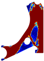
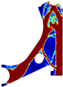
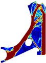
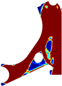
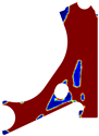
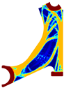
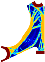
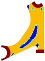
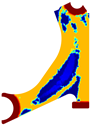
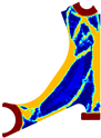
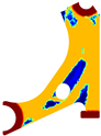
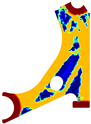
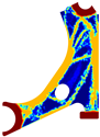
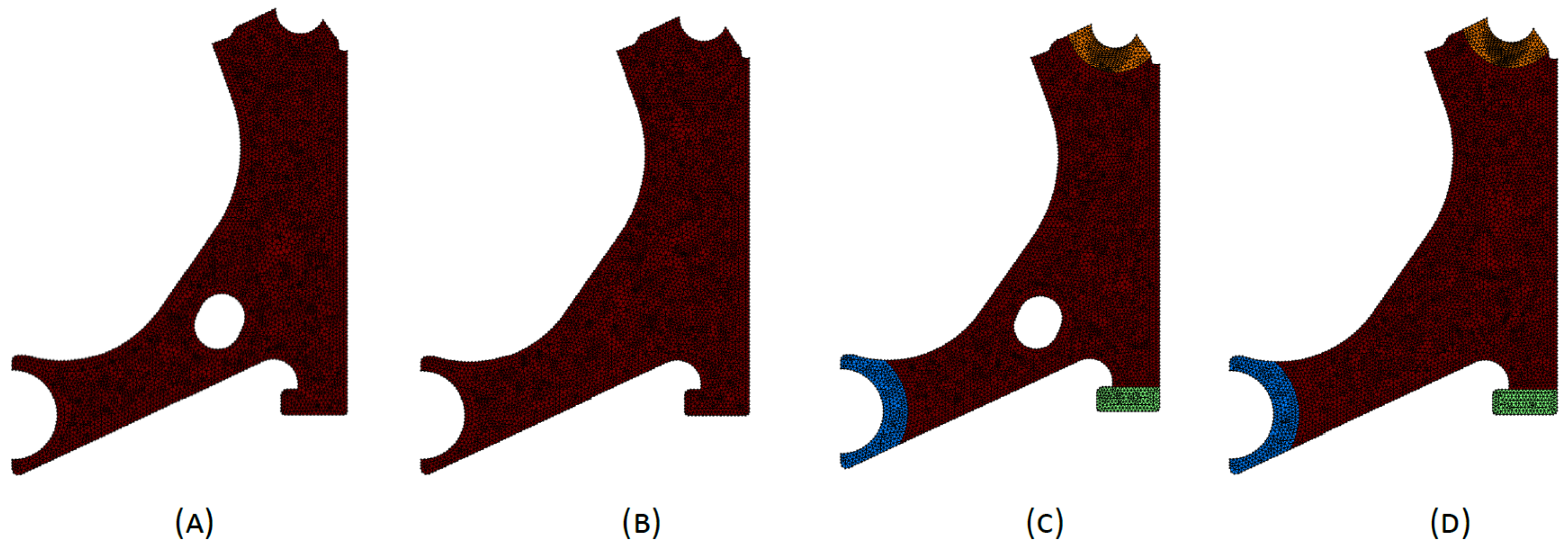
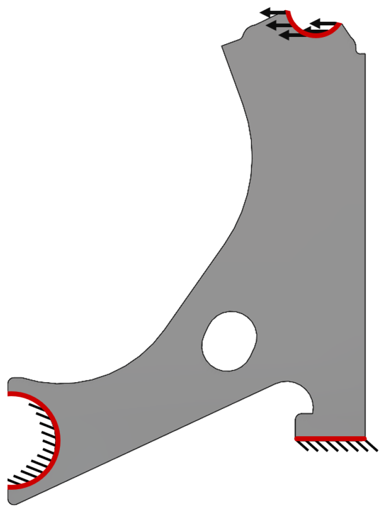
The objective of the present study is to employ a bio-inspired bi-evolutionary optimisation algorithm for a suspension control arm. The control arm design is based on the geometry of existent industry-standard suspension arms. In the field of automotive mechanical construction, product development heavily relies on design philosophies informed by engineers’ empirical knowledge. By applying automated techniques to selectively remove material from specific stressed components, it becomes feasible to achieve designs that align with the manufacturer’s requirements while significantly reducing mass. Additionally, recent literature indicates a preference for meshless methods, which not only serve as a viable alternative to FEM but also offer potential advantages [21,22].

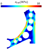
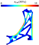
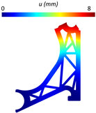
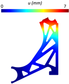
The paper begins with a review and brief explanation of the studied numerical method, the RPIM. Next, the numerical procedures of a traditional bi-evolutionary algorithm are examined. Additionally, a parallel is drawn between these procedures and the concept of bone remodelling. The article proceeds to conduct a numerical study. The optimisation algorithm is applied to the control arm. The topologies are designed using industry-standard philosophies for this specific component. A linear-static analysis follows, comparing the stiffness, specific stiffness, displacement, and maximum von Mises stress values among the different designed models. Finally, the last section summarises the findings and revisits the conclusions drawn throughout this numerical study.

2. Radial Point Interpolation Method

Similar to most numerical node-dependent discretisation methods, the majority of meshless methods follow a common procedure. The main differences between meshless methods and the standard and well-known FEM can be found at the pre-processing phase [7]. In opposition to FEM, which discretizes the problem domain with elements (containing nodes and integration points), meshless methods discretize the problem domain using only a nodal set. In meshless methods there are no pre-established connections between the discretization nodes. Such connection is enforced by some mathematical concept (radial search, natural neighbours, etc.) [7]. Also, the background integration points of meshless formulations can be constructed using node-independent or node-dependent rules, allowing a higher flexibility in their distribution along the problem domain [7]. Regarding the shape function construction, contrasting with FEM, meshless methods are able to apply distinct functions to build their shape functions, such as Moving Least Squares, Point Interpolation, Polynomial Interpolation, Sibson Interpolation, etc. [7]. Thus, next, in order to understand the general meshless procedure, a general overview is provided.

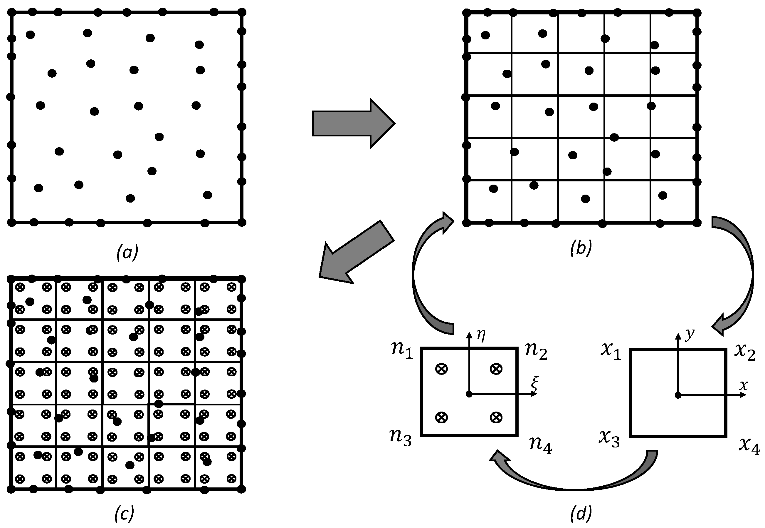
In meshless formulations, first, the solid domain is discretised with a nodal set, and the essential and natural boundaries are established. Following discretisation, it is necessary to construct a cloud of background integration points, covering the complete solid domain. The integration points can be obtained using the same procedure as FEM. First, integration cells are constructed, discretising the complete solid domain, and then the integration points are obtained following the Gauss–Legendre quadrature integration technique [7]. Each cell is subsequently transformed into a unit square using a parametric transformation (Figure 1). This transformation allows for the distribution of integration points within the resulting isoparametric square [7,17].

Once the integration mesh is established, the next step involves defining the nodal connectivity. In FEM, element definitions dictate nodal connectivity. However, meshless methods, as mentioned earlier, rely on influence domains rather than elements. Nodal connectivity is established by overlapping these influence domains. Finding these domains involves searching for nodes within a specific area or volume (depending on the problem’s spatial dimension). This approach, due to its simplicity and low computational cost, is widely used in various meshless methods like RPIM, EFGM, MLPG, and RKPM. It is important to consider the impact of domain size and shape on the method’s performance to achieve accurate and satisfactory solutions. While the literature suggests a single optimal size for influence domains is not feasible, a fixed reference dimension is often adopted. Each integration point ${\mathbf{x}}_{\mathbf{I}}$ searches for its closest nodes, forming its own influence domain. For the RPIM, the literature recommends between nine and sixteen nodes inside each influence domain [7].

In order to establish the system of equations, it is necessary to construct the shape functions. To obtain them, RPIM uses the radial point interpolating technique [7,17]. Considering a function, $u\left(\mathbf{x}\right)$, defined within the domain $\mathsf{\Omega }\in {\mathbb{R}}^2$. The domain is discretised by a set of N nodes, denoted by $\mathbf{X}=\{{\mathbf{x}}_1,{\mathbf{x}}_2,\cdots ,{\mathbf{x}}_N\}$. It can be further assumed that only the nodes located within the influence domain of a specific point of interest, ${\mathbf{x}}_I$, have an impact on the value of the function, $\mathbf{u}\left({\mathbf{x}}_I\right)$, at that point:

$$u\left({\mathbf{x}}_I\right)=\sum _{i=1}^n{R}_i\left({\mathbf{x}}_I\right)a_i\left({\mathbf{x}}_I\right)+\sum _{j=1}^m{p}_j\left({\mathbf{x}}_I\right)b_j\left({\mathbf{x}}_I\right)=\left\{{\mathbf{R}}^{\mathbf{T}}\left({\mathbf{x}}_I\right),{\mathbf{p}}^{\mathbf{T}}\left({\mathbf{x}}_I\right)\right\}\left\{\begin{array}{c}\mathbf{a}\\ \mathbf{b}\end{array}\right\},$$

(1)

where $R_i\left({\mathbf{x}}_I\right)$ represents a radial basis function (RBF), n and m stand for the number of nodes within the influence domain of ${\mathbf{x}}_I$ and the number of monomials of the polynomial basis function, respectively, and $a_i\left({\mathbf{x}}_I\right)$ and $b_j\left({\mathbf{x}}_I\right)$ represent non-constant coefficients of $R_i\left({\mathbf{x}}_I\right)$ and $p_j\left({\mathbf{x}}_I\right)$, respectively. Several radial basis functions are available in the literature [7], and many have been explored and developed over time. This work will utilise the multiquadratics (MQ) RBF, first introduced by Hardy [23]. This function is widely recognised as yielding superior results and is often paired with RPI [7]. The MQ RBF can be described as follows:

$$R_i\left({\mathbf{x}}_I\right)=R\left(r_{Ii}\right)={(r_{Ii}^2+c^2)}^p$$

(2)

for which,

$$r_{Ii}=\sqrt{{(x_i-x_I)}^2+{(y_i-y_I)}^2}.$$

(3)

The literature shows that shape parameters c and p considerably influence the shape of the final interpolation function and therefore the accuracy of the final results [7,17]. Therefore, following the literature recommendation, in this work, the following shape parameters are assumed: $c=1.42$ and $p=1.03$ [7,17]. These values will allow us to ensure that the constructed shape functions actually possess the delta Kronecker property. To ensure a unique approximation, the following additional system of equations is introduced:

$$\sum _{i=1}^n{p}_j\left(x_i\right)a_i\left(x_i\right)=0,j=1,2,...,m.$$

(4)

With Equations (1) and (4), it is possible to write

$$\left\{\begin{array}{c}\left[\begin{array}{c}{u}_1\\ u_2\\ ⋮\\ u_n\end{array}\right]\\ \left[\begin{array}{c}0\\ 0\\ 0\end{array}\right]\end{array}\right\}=\left[\begin{array}{cc}\left[\begin{array}{cccc}R\left(r_{11}\right)& R\left(r_{12}\right)& \cdots & R\left(r_{1n}\right)\\ R\left(r_{21}\right)& R\left(r_{22}\right)& \cdots & R\left(r_{2n}\right)\\ ⋮& ⋮& & ⋮\\ R\left(r_{n1}\right)& R\left(r_{n2}\right)& \cdots & R\left(r_{nn}\right)\end{array}\right]& \left[\begin{array}{ccc}1& x_1& y_1\\ 1& x_2& y_2\\ ⋮& ⋮& ⋮\\ 1& x_n& y_n\end{array}\right]\\ \left[\begin{array}{cccc}1& 1& \cdots & 1\\ x_1& x_2& \cdots & x_n\\ y_1& y_2& \cdots & y_n\end{array}\right]& \left[\begin{array}{ccc}0& 0& 0\\ 0& 0& 0\\ 0& 0& 0\end{array}\right]\end{array}\right]\left\{\begin{array}{c}\left[\begin{array}{c}{a}_1\\ a_2\\ ⋮\\ a_n\end{array}\right]\\ \left[\begin{array}{c}{b}_1\\ b_2\\ b_3\end{array}\right]\end{array}\right\},$$

(5)

which allows us to obtain the non-constant coefficients $a_i\left({\mathbf{x}}_I\right)$ and $b_j\left({\mathbf{x}}_I\right)$:

$$\left\{\begin{array}{c}\left[\begin{array}{c}{u}_1\\ u_2\\ ⋮\\ u_n\end{array}\right]\\ \left[\begin{array}{c}0\\ 0\\ 0\end{array}\right]\end{array}\right\}=\mathbf{G}\left\{\begin{array}{c}\left[\begin{array}{c}{a}_1\\ a_2\\ ⋮\\ a_n\end{array}\right]\\ \left[\begin{array}{c}{b}_1\\ b_2\\ b_3\end{array}\right]\end{array}\right\}⟹\left\{\begin{array}{c}\left[\begin{array}{c}{a}_1\\ a_2\\ ⋮\\ a_n\end{array}\right]\\ \left[\begin{array}{c}{b}_1\\ b_2\\ b_3\end{array}\right]\end{array}\right\}={\mathbf{G}}^{-}1\left\{\begin{array}{c}\left[\begin{array}{c}{u}_1\\ u_2\\ ⋮\\ u_n\end{array}\right]\\ \left[\begin{array}{c}0\\ 0\\ 0\end{array}\right]\end{array}\right\}={\mathbf{G}}^{-}1\left\{\begin{array}{c}{\mathbf{u}}_s\\ \mathbf{0}\end{array}\right\}.$$

(6)

Incorporating $a_i\left({\mathbf{x}}_I\right)$ and $b_j\left({\mathbf{x}}_I\right)$ into Equation (1), the following interpolation is achieved:

$$\mathbf{u}\left({\mathbf{x}}_I\right)=\left\{{\mathbf{R}}^{\mathbf{T}}\left({\mathbf{x}}_I\right),{\mathbf{p}}^T\left({\mathbf{x}}_I\right)\right\}{\mathbf{G}}^{-\mathbf{1}}\left\{\begin{array}{c}{\mathbf{u}}_{\mathbf{s}}\\ \mathbf{0}\end{array}\right\}=\phi \left({\mathbf{x}}_I\right){\mathbf{u}}_{\mathbf{s}},$$

(7)

being the shape function defined as

$$\mathit{\phi }\left({\mathbf{x}}_I\right)=\left\{{\mathbf{R}}^T\left({\mathbf{x}}_I\right),{\mathbf{p}}^{\mathbf{T}}\left({\mathbf{x}}_I\right)\right\}{\mathbf{G}}^{-1}=\left\{{\phi }_1\left({\mathbf{x}}_I\right),{\phi }_2\left({\mathbf{x}}_I\right),\cdots ,{\phi }_n\left({\mathbf{x}}_I\right)\right\}.$$

(8)

In elasticity, the equilibrium conditions can be represented by the following system of partial differential equations:

$$\nabla \mathit{\sigma }+\mathbf{b}=0,$$

(9)

where ∇ represents the nabla operator, $\mathit{\sigma }$ the Cauchy stress tensor, and $\mathbf{b}$ the body force vector. The boundary surface can be divided into two types of boundaries:

• Natural boundaries (${\Gamma }_t$), where $\sigma \mathbf{n}=\overline{\mathbf{t}}$.
• Essential boundaries (${\Gamma }_u$), where $\mathbf{u}=\overline{\mathbf{u}}$.

where $\overline{\mathbf{u}}$ represents the prescribed displacement vector on the essential boundary, ${\Gamma }_u$. Similarly, $\overline{\mathbf{t}}$ denotes the traction force applied on the natural boundary, ${\Gamma }_t$, and $\mathbf{n}$ represents its outward normal unit vector.

The Cauchy stress tensor $\mathit{\sigma }$, usually represented in the Voigt notation (Equation (10)), and the strain $\mathit{\epsilon }$ (Equation (11)) can be related with Hooke’s law: $\mathit{\sigma }=\mathbf{c}·\mathit{\epsilon }$, being the strain state obtained from the displacement field: $\mathit{\epsilon }=\mathbf{L}·\mathbf{u}$. In a full 3D problem, the differential operator $\mathbf{L}$ and the material constitutive matrix $\mathbf{c}$ are represented as shown in Equations (12) and (13), respectively:

$$\mathit{\sigma }={\left\{\begin{array}{cccccc}{\sigma }_{xx}& {\sigma }_{yy}& {\sigma }_{zz}& {\tau }_{xy}& {\tau }_{yz}& {\tau }_{zx}\end{array}\right\}}^T,$$

(10)

$$\mathit{\epsilon }={\left\{\begin{array}{cccccc}{\epsilon }_{xx}& {\epsilon }_{yy}& {\epsilon }_{zz}& {\gamma }_{xy}& {\gamma }_{yz}& {\gamma }_{zx}\end{array}\right\}}^T,$$

(11)

$$\mathbf{L}={\left[\begin{array}{cccccc}{\displaystyle \frac{\partial }{\partial x}}& 0& 0& {\displaystyle \frac{\partial }{\partial y}}& 0& {\displaystyle \frac{\partial }{\partial z}}\\ 0& {\displaystyle \frac{\partial }{\partial y}}& 0& {\displaystyle \frac{\partial }{\partial x}}& {\displaystyle \frac{\partial }{\partial z}}& 0\\ 0& 0& {\displaystyle \frac{\partial }{\partial z}}& 0& {\displaystyle \frac{\partial }{\partial y}}& {\displaystyle \frac{\partial }{\partial x}}\end{array}\right]}^T,$$

(12)

$$\mathbf{c}={\mu }_1\left[\begin{array}{cccccc}1& v& v& 0& 0& 0\\ v& 1& v& 0& 0& 0\\ v& v& 1& 0& 0& 0\\ 0& 0& 0& {\mu }_2& 0& 0\\ 0& 0& 0& 0& {\mu }_2& 0\\ 0& 0& 0& 0& 0& {\mu }_2\end{array}\right],$$

(13)

where ${\mu }_1={\displaystyle \frac{E}{1-v^2}}$ and ${\mu }_2={\displaystyle \frac{1-v}{2}}$. The selection of a methodology for approximating solutions to partial differential equations hinges on the intended application. Within computational mechanics, both strong and weak formulations are widely used approximation methods. While the strong form offers a potentially more direct and accurate approach in certain cases, it can become challenging to implement for problems of greater complexity. In these scenarios, due to its ability to generate a more robust system of equations, using the weak form is more advantageous. Thus, assuming the virtual work principle, the energy conservation is imposed:

$$\mathsf{\Psi }={\int }_{\mathsf{\Omega }}\delta {\mathit{\epsilon }}^T\mathit{\sigma }d\mathsf{\Omega }-{\int }_{\mathsf{\Omega }}\delta {\mathbf{u}}^T\mathit{\sigma }b\mathsf{\Omega }-{\int }_{{\Gamma }_t}\delta {\mathbf{u}}^T\mathbf{t}d\Gamma =0,$$

(14)

which allows, after standard manipulation [7], to obtain the following expression:

$$\mathsf{\Psi }=\delta {\mathbf{u}}^T(\mathbf{K}·\mathbf{u}-{\mathbf{f}}_{\mathbf{b}}-{\mathbf{f}}_{\mathbf{t}})=0,$$

(15)

leading to the simplified expression: $\mathbf{K}·\mathbf{u}={\mathbf{f}}_{\mathbf{b}}+{\mathbf{f}}_{\mathbf{t}}$. In this equation, $\mathbf{K}$ represents the global stiffness matrix, which can be expressed as follows:

$$\mathbf{K}={\int }_{\mathsf{\Omega }}{\mathbf{B}}^{\mathbf{T}}·\mathbf{c}·\mathbf{B}d\mathsf{\Omega }=\sum _{i=1}^{n_Q}\mathbf{B}{\left({\mathbf{x}}_I\right)}^{\mathbf{T}}·\mathbf{c}·\mathbf{B}\left({\mathbf{x}}_I\right)\widehat{w_I},$$

(16)

being $n_Q$, the number of integration points discretising the domain and $\widehat{w_I}$ their corresponding integration weight. The deformability matrix $\mathbf{B}$ can be defined as follows:

$$\mathbf{B}=\left[\begin{array}{ccccccc}{\displaystyle \frac{\partial {\phi }_1\left({\mathbf{x}}_I\right)}{\partial x}}& 0& 0& \cdots & {\displaystyle \frac{\partial {\phi }_n\left({\mathbf{x}}_I\right)}{\partial x}}& 0& 0\\ 0& {\displaystyle \frac{\partial {\phi }_1\left({\mathbf{x}}_I\right)}{\partial y}}& 0& \cdots & 0& {\displaystyle \frac{\partial {\phi }_n\left({\mathbf{x}}_I\right)}{\partial y}}& 0\\ 0& 0& {\displaystyle \frac{\partial {\phi }_1\left({\mathbf{x}}_I\right)}{\partial z}}& \cdots & 0& 0& {\displaystyle \frac{\partial {\phi }_n\left({\mathbf{x}}_I\right)}{\partial z}}\\ {\displaystyle \frac{\partial {\phi }_1\left({\mathbf{x}}_I\right)}{\partial y}}& {\displaystyle \frac{\partial {\phi }_1\left({\mathbf{x}}_I\right)}{\partial x}}& 0& \cdots & {\displaystyle \frac{\partial {\phi }_n\left({\mathbf{x}}_I\right)}{\partial y}}& {\displaystyle \frac{\partial {\phi }_n\left({\mathbf{x}}_I\right)}{\partial x}}& 0\\ 0& {\displaystyle \frac{\partial {\phi }_1\left({\mathbf{x}}_I\right)}{\partial z}}& {\displaystyle \frac{\partial {\phi }_1\left({\mathbf{x}}_I\right)}{\partial y}}& \cdots & 0& {\displaystyle \frac{\partial {\phi }_n\left({\mathbf{x}}_I\right)}{\partial z}}& {\displaystyle \frac{\partial {\phi }_n\left({\mathbf{x}}_I\right)}{\partial y}}\\ {\displaystyle \frac{\partial {\phi }_1\left({\mathbf{x}}_I\right)}{\partial z}}& 0& {\displaystyle \frac{\partial {\phi }_1\left({\mathbf{x}}_I\right)}{\partial x}}& \cdots & {\displaystyle \frac{\partial {\phi }_n\left({\mathbf{x}}_I\right)}{\partial z}}& 0& {\displaystyle \frac{\partial {\phi }_n\left({\mathbf{x}}_I\right)}{\partial x}}\end{array}\right].$$

(17)

From Equation (14), it is possible to express the body force vector (denoted by ${\mathbf{f}}_b$) and the external force vector (denoted by ${\mathbf{f}}_t$) as follows:

$${\mathbf{f}}_b={\int }_{\mathsf{\Omega }}{\mathbf{H}}^{\mathbf{T}}·\mathbf{b}d\mathsf{\Omega }=\sum _{i=1}^{n_Q}\mathbf{H}{\left({\mathbf{x}}_I\right)}^{\mathbf{T}}·\mathbf{b}·\widehat{w_I},$$

(18)

$${\mathbf{f}}_t={\int }_{\Gamma }{\mathbf{H}}^{\mathbf{T}}·\overline{\mathbf{t}}d\Gamma =\sum _{i=1}^{n_Q^{*}}\mathbf{H}{\left({\mathbf{x}}_I\right)}^{\mathbf{T}}·\mathbf{f}·\widehat{w_I^{*}},$$

(19)

where $n_Q^{*}$ denotes the number of integration points defining the boundary where this force is applied to, and $\widehat{w_I^{*}}$ their corresponding integration weight. Finally, $\mathbf{H}$ represents the interpolation matrix:

$$\mathbf{H}=\left[\begin{array}{ccccccc}{\phi }_1\left({\mathbf{x}}_I\right)& 0& 0& \cdots & {\phi }_n\left({\mathbf{x}}_I\right)& 0& 0\\ 0& {\phi }_1\left({\mathbf{x}}_I\right)& 0& \cdots & 0& {\phi }_n\left({\mathbf{x}}_I\right)& 0\\ 0& 0& {\phi }_1\left({\mathbf{x}}_I\right)& \cdots & 0& 0& {\phi }_n\left({\mathbf{x}}_I\right)\end{array}\right].$$

(20)

The Kronecker delta property inherent to RPI shape functions allows for the direct imposition of essential boundary conditions on the stiffness matrix, $\mathbf{K}$. Thus, the same numerical techniques applied to standard FEM can be used with RPIM. If plane stress is assumed, the problem reduces to a 2D analysis. The presented 3D formulation is still valid; however, all components associated with the $Oz$ direction are removed. Thus, regarding the stress and strain vectors,

$$\mathit{\sigma }={\left\{\begin{array}{ccc}{\sigma }_{xx}& {\sigma }_{yy}& {\tau }_{xy}\end{array}\right\}}^T,$$

(21)

$$\mathit{\epsilon }={\left\{\begin{array}{ccc}{\epsilon }_{xx}& {\epsilon }_{yy}& {\gamma }_{xy}\end{array}\right\}}^T.$$

(22)

The constitutive matrix is reduced to

$$\mathbf{c}={\mu }_1\left[\begin{array}{ccc}1& v& 0\\ v& 1& 0\\ 0& 0& {\mu }_2\end{array}\right]$$

(23)

and the deformability and interpolation matrices become

$$\mathbf{B}=\left[\begin{array}{ccccc}{\displaystyle \frac{\partial {\phi }_1\left({\mathbf{x}}_I\right)}{\partial x}}& 0& \cdots & {\displaystyle \frac{\partial {\phi }_n\left({\mathbf{x}}_I\right)}{\partial x}}& 0\\ 0& {\displaystyle \frac{\partial {\phi }_1\left({\mathbf{x}}_I\right)}{\partial y}}& \cdots & 0& {\displaystyle \frac{\partial {\phi }_n\left({\mathbf{x}}_I\right)}{\partial x}}\\ {\displaystyle \frac{\partial {\phi }_1\left({\mathbf{x}}_I\right)}{\partial y}}& {\displaystyle \frac{\partial {\phi }_1\left({\mathbf{x}}_I\right)}{\partial x}}& \cdots & {\displaystyle \frac{\partial {\phi }_n\left({\mathbf{x}}_I\right)}{\partial y}}& {\displaystyle \frac{\partial {\phi }_n\left({\mathbf{x}}_I\right)}{\partial y}}\end{array}\right],$$

(24)

$$\mathbf{H}=\left[\begin{array}{ccccc}{\phi }_1\left({\mathbf{x}}_I\right)& 0& \cdots & {\phi }_n\left({\mathbf{x}}_I\right)& 0\\ 0& {\phi }_1\left({\mathbf{x}}_I\right)& \cdots & 0& {\phi }_n\left({\mathbf{x}}_I\right)\end{array}\right].$$

(25)

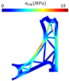
3. Topology Optimisation with a Bi-Directional Bone Remodelling Algorithm

Within computational mechanics, topological optimisation stands as a prominent optimisation method due to its capacity to generate innovative and highly efficient designs. This approach strategically distributes material within a structure, resulting in optimised shapes and layouts that meet specific performance requirements. These requirements can encompass factors such as strength, stiffness, or other mechanically relevant metrics. Consider a common topological optimisation problem applied to a structure, where the goal is to achieve a design with maximum rigidity while adhering to a constraint on the structure’s mass. Mathematically, this translates to minimising the average compliance subject to a constraint on the material’s weight, which can be expressed as

$$\begin{array}{ccc}& MinimizeC={\displaystyle \frac{1}{2}}·{\mathbf{f}}^T·\mathbf{u}\hfill & \\ & s.t.:W^{*}-\sum _{i=1}^n{W}_i{x}_i=0\hfill & \\ & x_i=0or1\hfill \end{array}$$

(26)

where C represents the average compliance of the structure, $W^{*}$ the mass of the selected structure, and $W_i$ the mass of node i. The design variable $x_i$ indicates the presence ($x_i=1)$ or absence ($x_i=0)$ of a node in the layout of the defined domain.

3.1. Bi-Directional Evolutionary Structural Optimisation

Evolutionary computation, inspired by biological evolution, utilises selection, reproduction, and variation mechanisms to find optimal solutions for complex problems [24]. Compared with traditional optimisation techniques, evolutionary methods offer greater robustness, exploration capabilities, and flexibility. These attributes make them well-suited for tackling intricate problems with challenging cost functions. In recent years, methods like Evolutionary Structural Optimisation (ESO), developed by Xie and Steven [25], have gained widespread application in structural optimisation problems. This iterative technique removes material deemed inefficient or redundant from a specific domain to achieve an optimal design. While the ESO method demonstrates widespread application and popularity, it does possess limitations that have motivated the exploration of alternative techniques [26]. To enhance the solution viability achieved through optimisation, the concept of a bidirectional algorithm emerged. This approach would not only remove material in low-stress areas but also introduce material to reinforce high-stress regions. This led to the development of the Bi-Directional Evolutionary Structural Optimisation (BESO) method, drawing inspiration from both ESO’s material removal capabilities and the additive material functionalities of the Additive Evolutionary Structural Optimisation (AESO) method [27]. BESO facilitates a more comprehensive exploration of the design domain, potentially leading to superior identification of the global minimum.

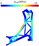
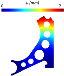
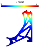
The elasto-static analysis step initiates each optimisation iteration and returns the displacement, strain, and stress fields. This allows for the calculation of the equivalent von Mises stress for each point, along with the cubic average of the entire von Mises stress field. This average serves as a reference to identify potential locations of abrupt stress variations. High stress values influence the cubic average, while low stress values have minimal impact.

$$\overline{\sigma }\left(x_I\right)=\sqrt{{\displaystyle \frac{{({\sigma }_{xx}-{\sigma }_{yy})}^2+{({\sigma }_{yy}-{\sigma }_{zz})}^2+{({\sigma }_{zz}-{\sigma }_{xx})}^2+6({\tau }_{xy}^2+{\tau }_{yz}^2+{\tau }_{zx}^2)}{2}}}$$

(27)

$${\overline{\sigma }}_{cube}=\sqrt[3]{{\displaystyle \frac{1}{n_Q}}\sum _{i=1}^{n_Q}\overline{\sigma }{\left({\mathbf{x}}_I\right)}^3}$$

(28)

A penalty system is implemented to designate a specific parameter, mass density in this case, to each integration point. The penalty values typically range from $\xi \in [{10}^{-3},1]$, where 1 signifies rewarded domains (solid material) and ${10}^{-3}$ signifies penalised domains (removed material). The performance of the BESO procedure hinges on the reward ratio, RR, and the penalty ratio, PR.

The procedure identifies the $n_Q^{RR}=RR·n_Q$ integration points with the highest $\sigma \left({\mathbf{x}}_I\right)$ (stress) and the $n_Q^{PR}=PR·n_Q$ integration points with the lowest $\sigma \left({\mathbf{x}}_I\right)$. The $n_Q^{RR}$ points are assigned a reward of $\xi \left({\mathbf{x}}_I\right)=1$, while the $n_Q^{PR}$ points receive a penalty of $\xi \left({\mathbf{x}}_I\right)={10}^{-3}$. A penalty parameter, $\eta \left({\mathbf{x}}_i\right)$, is then assigned to each node ${\mathbf{x}}_i$. For each integration point ${\mathbf{x}}_I$, the closest nodes update their penalty values using the expression $\eta {\left({\mathbf{x}}_i\right)}^{new}=0.5(\eta {\left({\mathbf{x}}_i\right)}^{old}+\xi \left({\mathbf{x}}_I\right))$. Once all nodes are updated, the penalty parameters for each integration point are recalculated to filter and smooth the selected values. This is achieved using the interpolation function $\xi \left({\mathbf{x}}_I\right)={\sum }_{i=1}^n{\phi }_i\left({\mathbf{x}}_I\right)·\eta \left({\mathbf{x}}_i\right)$, where n represents the number of nodes within the analysed influence domain of ${\mathbf{x}}_I$, and $\phi \left({\mathbf{x}}_I\right)$ represents the shape function vector of the integration point ${\mathbf{x}}_I$. After the first iteration, some $\xi$ values might deviate from one, indicating the absence of material. This prompts the process to proceed to the next iteration. In iteration j, the penalty parameters, $\xi$, are used to modify the material constitutive matrix. Consequently, the penalised constitutive material matrix, $c_p\left({\mathbf{x}}_I\right)=\xi \left({\mathbf{x}}_I\right)·c\left({\mathbf{x}}_I\right)$, is calculated.

In the subsequent iteration, $j+1$, the stiffness matrix is calculated using $c_p\left({\mathbf{x}}_I\right)$ instead of the original material matrix, $c\left({\mathbf{x}}_I\right)$. The same steps are repeated, leading to a new equivalent von Mises stress field. This new field is used to calculate the updated cubic average stress. A comparison is then made: ${\sigma }_{cubic}^j\ge \delta ·{\sigma }_{cubic}^{j-1}$. If the condition holds true, the integration points with $\xi \left({\mathbf{x}}_I\right)>\lambda$ are rewarded with $\xi \left({\mathbf{x}}_I\right)=1$. The penalty parameters are then recalculated, updating the material domain for the next iteration.

3.2. BESO-Inspired Bone Remodelling

This work employs a BESO-inspired bone remodelling analysis aiming at structural optimisation. Bone remodelling is a natural process where the bone’s shape adapts to applied stresses, improving its resistance to the imposed load. To predict this behaviour, researchers have developed stress-strain laws based on observations and experiments. These laws predict bone behaviour under various loading conditions and serve as the foundation for computational bone analysis. The selected model can considerably influence simulation results. Established models include Pauwels’ model [28], along with more recent models that incorporate additional factors or different approaches, such as Corwin’s [29] and Carter’s [30] models.

Similar to Pauwels’ model, Carter’s model necessitates a mechanical stimulus to trigger bone remodelling. This stimulus is computed based on the effective stress, which incorporates both the local stress and bone density, along with the number of load cycles experienced by the bone (represented by the exponent k). The magnitude of the stress has a direct impact on the remodelling stimulus; a higher stress level translates to a stronger stimulus for remodelling.

$$S_n\propto \sum _{i=1}^l{m}_i{\overline{{\sigma }_i}}^k$$

(29)

The model offers the flexibility to use either stress or strain energy as the optimisation criterion. Strain energy prioritises maximising the bone’s stiffness, its resistance to bending, while stress prioritises optimising the material’s strength. When using strain energy, the model relates the apparent bone density to the local strain energy it experiences. This allows for estimation of the bone’s density at a remodelling equilibrium, a state where bone resorption and formation are balanced.

$${\rho }_{app}\propto (\sum _{i=1}^l{m}_i{U}_i^k)$$

(30)

In cases where multi-directional stress is applied to the bone, the model combines the effects of each stress pattern into a single, unified direction. This direction, known as the normal vector (represented by $\mathbf{n}$), signifies the ideal alignment for the bone’s internal support structures (trabeculae) to achieve optimal strength. To determine this ideal direction, the model incorporates the normal stress acting on the entire bone, as described in Equation (31).

$$\overline{{\sigma }_n}\left(\mathbf{n}\right)={\left(\sum _{i=1}^l{\displaystyle \frac{m_i}{{\sum }_{j=1}^l}}{\overline{\sigma }}_{n_i}^k\left(\mathbf{n}\right)\right)}^{{\displaystyle \frac{1}{k}}}$$

(31)

For the present work, an original algorithm was developed and programmed. The algorithm was incorporated in the previous codes already developed by the research team, which employed an adaptation of Carter’s model for meshless methods developed by Belinha et al. [31]. This adaptation assumes that a mechanical stimulus, primarily represented by stress and potentially incorporating strain metrics, is the key driver of bone tissue remodelling. A comprehensive description of the entire model can be found in the work of Belinha [7]. Through the bone remodelling procedure described above, the process itself acts as a topological optimisation algorithm. At each iteration, only the points with high or low energy deformation density undergo density optimisation based on the mechanical stimulus. In order to update the critical variables during the optimisation process, the algorithm assumes a phenomenological law of bone tissue developed by Belinha [7]. More information and a detailed description of the algorithm can be found in the literature [7]. 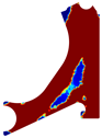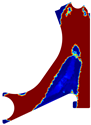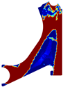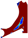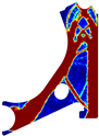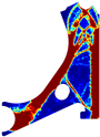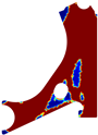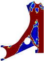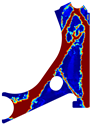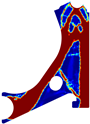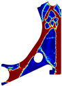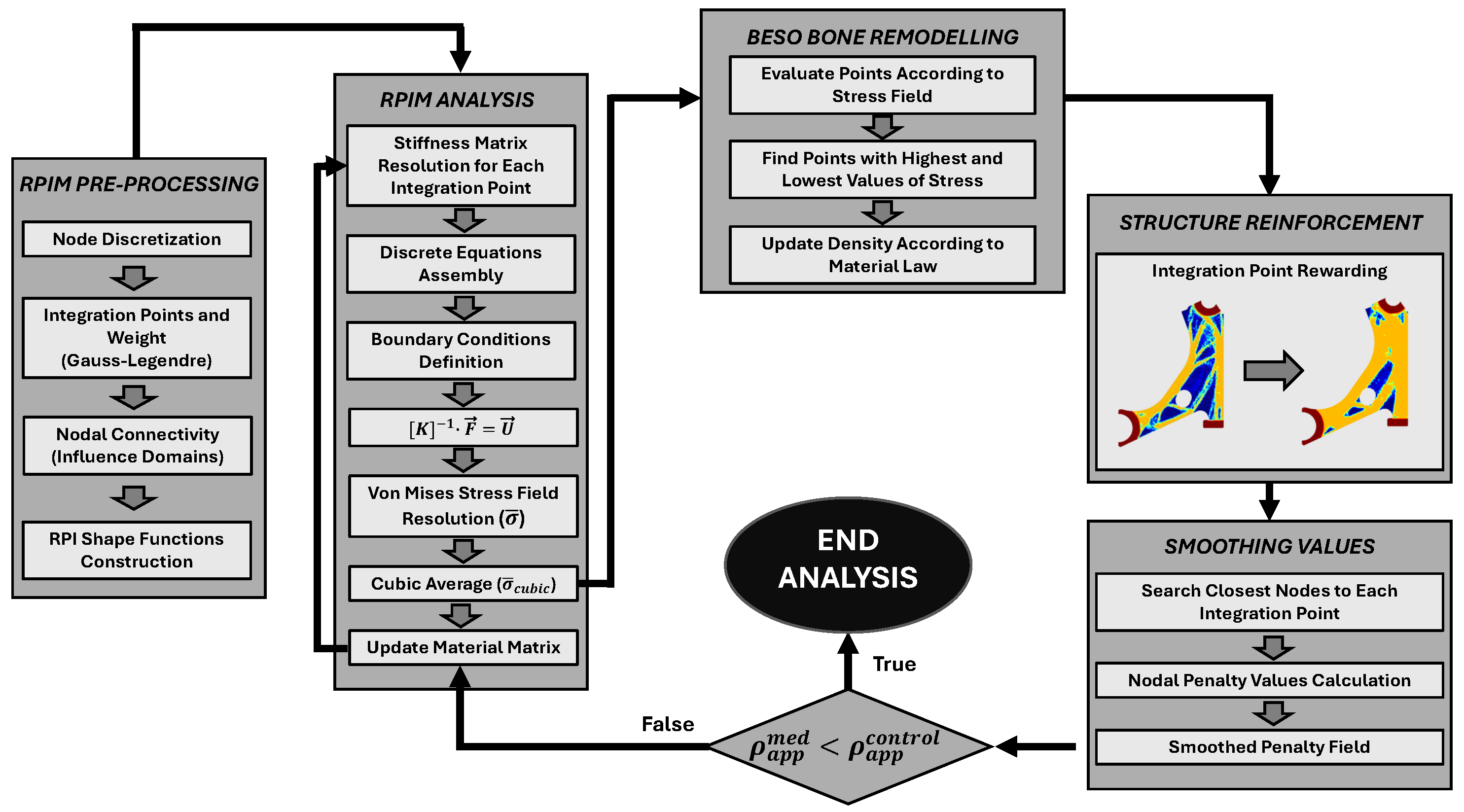Figure 2 illustrates a schematic representation of the optimisation topology algorithm inspired by the bone remodelling process, as implemented in the RPIM method. As illustrated in the flowchart, the structural optimisation algorithm used in this work is iterative. In each iteration, for a given material distribution, the stiffness matrix is computed and the resulting field variables (displacements, strains, and stresses) are determined. Next, the $N_Q·PR$ integration points with the lowest stress levels have their material densities reduced, consequently decreasing their mechanical properties. Here, $N_Q$ represents the total number of integration points, and $PR$ is the penalisation ratio defined at the start of the analysis. A similar procedure is applied to the $N_Q·RR$ integration points with the highest stress levels, increasing their material densities and, in turn, their mechanical properties. The value $RR$ is the reward ratio, also set at the beginning of the analysis.

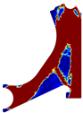
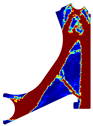
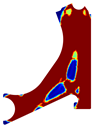
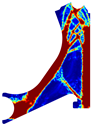
After these updates, the material distribution changes, and a new set of field variables is obtained, leading to a fresh remodelling scenario. This iterative remodeling continues until the average density of the model falls below a user-defined threshold.

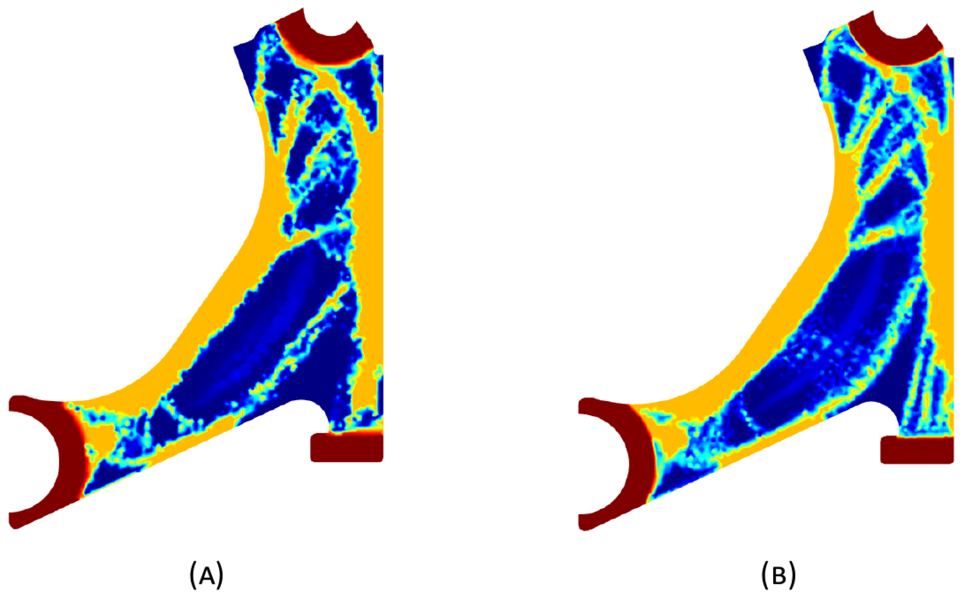
Because the FEM and RPIM formulations differ mathematically, they produce similar but not identical field variables when applied to the same material model. Moreover, given that the iterative optimisation algorithm’s solution at each stage depends on the previous iteration’s results, there is no straightforward guarantee that FEM and RPIM analyses will converge to the same solution.

4. Numerical Results

This section presents the numerical results obtained by optimising a vehicle’s control arm. We compare the results achieved using the previously described RPIM method with those obtained from the Finite Element Method (FEM). All numerical simulations employed a plane stress analysis approach, assuming the stress vector normal to the $xy$ plane is zero. In this work the following formulations were used to perform the optimisation analyses:

• FEM: three-node 2D linear triangular elements with constant strain;
• RPIM: triangular Gaussian integration scheme with $1\times 1$ integration points per triangular cell, influence domains with 16 nodes per integration point, MQ-RBF with shape parameters $c=1.42$ and $p=1.03$, and linear polynomial basis function.

4.1. Control Arm Optimization

This subsection applies a BESO-like algorithm, inspired by bone remodelling applications in which the output is not a binary density structure, to optimise the stiffness of a suspension control arm by making use of the FEM and the NNRPIM as solvers. The optimisation parameters were chosen based on values previously documented in the literature [32]. Penalisation ratios (PRs) of 5% and 10% are applied, and the reward ratio (RR) will be kept at all moments to 1%. The effective von Mises stress criterion is used exclusively. The process began by finding a 3D CAD model of a relatively functional control arm. The geometry was then simplified to a 2D format using Solidworks^® Student Edition 2023 SP2.1 (Figure 3). The created 2D sketch was subsequently exported to FEMAP 2021.2 MP1 (student version licence) for mesh generation before being imported into the software developed by the research team written in Octave/Matlab (2023b).

Four different meshes were built, corresponding to four distinct case studies that will be further analysed: a mesh D1 with the arm’s characteristic perforation (Figure 4A), a mesh D2 without the perforation (Figure 4B), a mesh D3 with perforation and material non-remodelling zones (Figure 4C), and a mesh D4 without perforation and with material non-remodelling zones (Figure 4D). The material non-remodelling zones, at the essential and natural boundary conditions, are necessary to ensure that these zones do not reduce its material density. By maintaining a homogeneous and continuous material distribution at the essential and natural boundary conditions, strain/stress concentrations are avoided in these sections, expectedly allowing for a smoother material remodelling.

The material properties considered were purely academic and do not represent a specific material. Thus, the following mechanical properties were assumed: Young’s modulus E = 1 MPa and Poisson’s ratio $\nu$ = 0.3. Respecting the control arm function, the essential and natural boundary conditions shown in Figure 5 were considered. At the circular surface, a distributed load of $f=1$ N/mm was applied. These boundary conditions replicate bending (flexion) of the component, a common mechanical behaviour experienced during the structure’s operation.

Table 1. Optimised solutions obtained with discretization D1. In each figure is indicated the mass at the iteration i ($m_i$) with respect to the initial mass ($m_o$).

PR	Method	Solution
5%	FEM	it. 8 mi = 86.06% mo	it. 15 mi = 77.00% mo	it. 24 mi = 63.73% mo	it. 33 mi = 51.89% mo
	RPIM	it. 8 mi = 88.25% mo	it. 15 mi = 77.29% mo	it. 24 mi = 63.79% mo	it. 33 mi = 53.81% mo
10%	FEM	it. 4 mi = 90.12% mo	it. 9 mi = 72.03% mo	it. 13 mi = 61.58% mo	it. 18 mi = 49.84% mo
	RPIM	it. 4 mi = 90.53% mo	it. 9 mi = 72.56% mo	it. 13 mi = 62.37% mo	it. 18 mi = 50.49% mo

,

Table 2. Optimised solutions obtained with discretization D2. In each figure is indicated the mass at the iteration i ($m_i$) with respect to the initial mass ($m_o$).

PR	Method	Solution
5%	FEM	it. 8 mi = 87.76% mo	it. 15 mi = 77.12% mo	it. 24 mi = 65.50% mo	it. 33 mi = 55.93% mo
	RPIM	it. 8 mi = 87.36% mo	it. 15 mi = 76.90% mo	it. 24 mi = 63.70% mo	it. 33 mi = 53.95% mo
10%	FEM	it. 4 mi = 90.24% mo	it. 9 mi = 72.08% mo	it. 13 mi = 62.16% mo	it. 18 mi = 50.81% mo
	RPIM	it. 4 mi = 90.34% mo	it. 9 mi = 72.27% mo	it. 13 mi = 62.30% mo	it. 18 mi = 50.80% mo

,

Table 3. Optimised solutions obtained with discretization D3. In each figure is indicated the mass at the iteration i ($m_i$) with respect to the initial mass ($m_o$).

PR	Method	Solution
5%	FEM	it. 8 mi = 88.11% mo	it. 15 mi = 78.53% mo	it. 24 mi = 65.57% mo	it. 30 mi = 60.49% mo
	RPIM	it. 8 mi = 88.04% mo	it. 15 mi = 78.64% mo	it. 24 mi = 66.69% mo	it. 30 mi = 61.71% mo
10%	FEM	it. 4 mi = 91.54% mo	it. 9 mi = 74.82% mo	it. 13 mi = 65.20% mo	it. 17 mi = 59.39% mo
	RPIM	it. 4 mi = 91.18% mo	it. 9 mi = 74.66% mo	it. 13 mi = 64.91% mo	it. 17 mi = 58.97% mo

and

Table 4. Optimised solutions obtained with discretization D4. In each figure is indicated the mass at the iteration i ($m_i$) with respect to the initial mass ($m_o$).

PR	Method	Solution
5%	FEM	it. 8 mi = 87.76% mo	it. 15 mi = 77.12% mo	it. 24 mi = 65.50% mo	it. 30 mi = 55.93% mo
	RPIM	it. 8 mi = 87.36% mo	it. 15 mi = 76.90% mo	it. 24 mi = 63.70% mo	it. 30 mi = 53.95% mo
10%	FEM	it. 4 mi = 90.24% mo	it. 9 mi = 72.08% mo	it. 13 mi = 62.16% mo	it. 17 mi = 50.81% mo
	RPIM	it. 4 mi = 90.34% mo	it. 9 mi = 72.27% mo	it. 13 mi = 62.30% mo	it. 17 mi = 50.80% mo

present the obtained topologies for the different meshes and control arm arrangements considered. Analysing the design solutions allows us to understand that the perforation in the control arm is situated in the null stress location. Thus, this indicated that this perforation serves solely to reduce the component’s overall mass. Examining real-world suspension assemblies further strengthens this observation, as the perforation often appears without hindering the component’s functionality. The optimisation results suggest the possibility of even more substantial material removal compared with the original design. The obtained density fields consistently displayed highly binary structures (clear distinctions between solid and practically void regions) across all cases. Notably, a penalisation ratio (PR) of 5% yielded the most promising solutions. These solutions exhibited a clear improvement and better connectivity between generated sections, particularly evident when comparing the initial and final iterations of both methods. There were slight differences in the final iteration volume fraction between the FEM and RPIM results.

To facilitate the visual comparison, two solutions from each method were selected from Table 3. Figure 6 shows two solutions of the previously presented optimisation of the initially solid control arm with density reduction restriction in the boundary conditions zone for $PR=5\%$. The chosen iteration was the very last one, in order to analyse the final result of the used algorithm.

Since FEM and RPIM formulations are different (from a mathematical point of view), for the same material model they lead to different variable fields (very close, but different). Because the adopted optimisation algorithm is iterative, and the solution of the next iteration is dependent on the solution of the previous iteration, it is not straightforward that FEM and RPIM analyses tend to the same solution. In this work, it was found that FEM and RPIM analyses allow us to obtain similar results, but with observable differences. For instance, observing just the last column of Table 1, it is possible to observe that for a $PR=5\%$, RPIM allows one to achieve in the upper part of the model a more defined trabecular arrangement (the trabeculae are more noticeable). Additionally, in the centre part of the model, a thin diagonal trabecula appears in both FEM and RPIM. However, a closer look allows us to observe that RPIM is capable of suggesting a capital, connecting the thin diagonal trabecula to the thick centre diagonal trabecula (which will better distribute the stresses). The same phenomenon can be observed in Table 2 ($PR=5\%$). In Table 3 and Table 4, comparing the last column results, it is possible to observe that RPIM allows for once again more defined trabeculae arrangement (all the trabeculae predicted by the RPIM are much more defined than the ones predicted by the FEM).

Visually, the RPIM solution exhibits a clearer truss-like structure and a wider range of intermediate densities compared with the FEM solution. Both of these characteristics are potentially advantageous for additive manufacturing, as they can influence the component’s structural performance.

4.2. Topology Design and Structural Analysis

Four new models were created based on the previously optimised control arm design, aiming to translate such findings into practical geometries suitable for manufacturing. These models incorporated key features from the optimisation results and considered common design practices for control arms (Figure 7). Thus, Model 1 is a reinforced version of the solutions presented in Table 2. Model 2 is a commonly used design for the control arm. Model 3 is a reinforced version of the solutions shown in Table 4, and Model 4 is a variation of Model 3 with a modified boundary contour. This modification involves a 50% increase (1.5 times) in the boundary contour thickness compared with the baseline model. The localised increased thickness is achieved by a 6mm outward offset from the original boundary contour, which was set to 1.5 times the nominal value of the remaining part.

With the respective design modelling completed, the essential and natural boundary conditions used in the optimisation process were imposed, and static linear analyses were performed with each model shown in Figure 7 and also with a completely solid model.

Table 5. Displacement and von Mises stress fields obtained for the solid control arm.

	FEM	RPIM
${\sigma }_{VM}$
$∥u∥$

presents the displacement and von Mises stress fields obtained for the solid model using both FEM and RPIM. The comparison revealed minimal discrepancies between the methods.

Table 6. Displacement and von Mises stress fields obtained with FEM for each one of the four models considered.

	Model 1	Model 2	Model 3	Model 4
${\sigma }_{VM}$
$∥u∥$

and

Table 7. Displacement and von Mises stress fields obtained with RPIM for each one of the four models considered.

	Model 1	Model 2	Model 3	Model 4
${\sigma }_{VM}$
$∥u∥$

show the obtained von Mises stress field and displacement field of each studied model for the FEM and RPIM analyses, respectively. Then,

Table 8. Results obtained with the model of the solid structure and with the proposed designed models M1 to M4.

		Solid Control Arm	Model 1	Model 2	Model 3	Model 4
$V_f^{\%}(\%)$		100	70.06	76.78	68.50	81.70
$∥u∥\left[\mathrm{mm}\right]$	FEM	5.408	8.505 (+57.27%)	7.422 (+37.24%)	8.689 (+60.67%)	7.165 (+32.49%)
	RPIM	5.420	8.478 (+56.42%)	7.476 (+37.93%)	8.790 (+62.18%)	7.374 (+36.05%)
${\sigma }_{max}^{VM}\left[\mathrm{Pa}\right]$	FEM	7.567	13.922 (+83.98%)	10.789 (+42.58%)	13.896 (+83.64%)	13.311 (+75.91%)
	RPIM	7.429	13.391 (+80.25%)	12.184 (+64.00%)	15.158 (+104.04%)	14.428 (+94.21%)
$K[\mathrm{N}/\mathrm{mm}]$	FEM	0.185	0.118 (−36.22%)	0.135 (−27.03%)	0.115 (−37.84%)	0.140 (−24.32%)
	RPIM	0.184	0.118 (−35.87%)	0.134 (−27.17%)	0.114 (−38.04%)	0.136 (−26.09%)
$K/V_f^{\%}[\mathrm{N}/\mathrm{mm}]$	FEM	0.185	0.168 (−9.19%)	0.175 (−5.41%)	0.168 (−9.19%)	0.171 (−7.57%)
	RPIM	0.184	0.168 (−7.70%)	0.174 (−5.43%)	0.166 (−9.78%)	0.166 (−9.78%)

summarises the structural values (obtained with the linear static analyses) and volume fractions of the designed models. Notice that K represents the directional stiffness of the component regarding the applied load. It is calculated with the following expression:

$$K={\displaystyle \frac{1}{n}}·\sum _{i=1}^n{\displaystyle \frac{f_i}{d_i}},$$

(32)

being n the number of nodes along the natural neighbour, $f_i$ the force applied at node $n_i$ of the natural boundary, along direction $Ox$, and $d_I$ is the displacement obtained at the same node $n_i$, along the same direction $Ox$. Based on the presented results, the following conclusions can be drawn:

• Comparing with the other proposed models, Model 2 shows the lower von Mises stress and higher stiffness. Additionally, its specific stiffness is close to the solid arm. Therefore, it appears that Model 2 shows the best mechanical performance. These results align with initial expectations, as the circular material removal promotes a more uniform stress distribution throughout the structure. Consequently, stress does not concentrate at specific points, leading to a reduction in the risk of failure and an overall increase in the model’s stiffness.
• Models 1 and 3 adopted similar design approaches, both employing a triangular material removal strategy, resulting in identical performance values. However, Model 1 allows for lower stress values. The thickness of the bar seems to be less important than its orientation. Therefore, the reason behind the best performance seems to be a multifactorial problem, depending on the bars’ orientation, thickness, and distribution.
• Model 4, a variation of Model 3 with a thicker outer contour (known as coating), displayed higher stiffness and lower maximum von Mises stress as anticipated (when directly compared with Model 3). However, due to the increased volume fraction associated with this reinforcement, the specific stiffness remained unchanged compared with Model 3.

It was verified that both formulations are capable of producing very similar results. With Table 6 and Table 7, it is possible to understand that FEM consistently predicts slightly lower stresses than RPIM formulation. This can be explained by the higher bending stiffness of the constant strain triangular element, well documented in the literature [33]. Nevertheless, the obtained stress distributions of both formulations are very close. Regarding the displacement field, it can be observed that both FEM and RPIM produce similar displacement fields. Concerning the compliance of each model, it can be calculated by inverting the directional stiffness K.

5. Conclusions

This work focused on applying the RPIM and comparing it with the well-established FEM for a modified bi-evolutionary topological optimisation algorithm inspired by the bone remodelling concept. The study investigated the topological optimisation of a generic automotive control arm. The initially constructed 3D model was converted to a simplified 2D layout. Evaluation of the obtained solutions revealed that RPIM-generated topologies with superior truss connections and a greater number of intermediate densities would considerably enhance the mechanical performance of a hypothetical part manufactured through additive manufacturing. Additionally, RPIM demonstrated acceptable convergence in traditional linear static analyses, suggesting its potential as a viable alternative to FEM in specific topological optimisation scenarios. Four designs were subsequently built based on a solution retrieved from the aforementioned algorithm, utilising material removal techniques commonly employed in the automotive industry for the component under study: a trussed design model, a model with circular material removal, a model with triangular removal, and a model replicating the previous one but with an increased outer thickness of 1.5 times the nominal thickness of the remaining model. A linear static analysis, conducted under the same conditions used in the optimisation algorithm, demonstrated that the design based on circular material removal exhibited the best stiffness and specific stiffness. This confirmed the initial hypothesis, as the circular shape facilitates a more uniform distribution of stresses throughout the structure, aligning with established mechanical design practices known to improve a structure’s mechanical performance. The trussed and triangular models displayed comparable behaviour due to the similarities in their material removal principles. As anticipated, the thickness-differentiated model exhibited lower displacement and consequently higher stiffness compared with the single-thickness model. However, the resulting increase in mass and total volume did not correspond to any improvement in specific stiffness relative to the model it was based on (model 3). Minor discrepancies were observed in the von Mises stress fields and maximum stress values obtained from the different methods. Moreover, both FEM and RPIM produce similar displacement values. The results here presented show that RPIM is capable of producing very close results to FEM, being a numerical alternative to FEM in such topological optimisation problems.

References

1. Oanta, E.; Raicu, A.; Menabil, B. Applications of the numerical methods in mechanical engineering experimental studies. IOP Conf. Ser. Mater. Sci. Eng. 2020, 916, 012074. [Google Scholar] [CrossRef]
2. Jones, D. Optimization in the Automotive Industry. In Optimization and Industry: New Frontiers; Springer: Boston, MA, USA, 2003. [Google Scholar] [CrossRef]
3. Witik, R.; Payet, J.; Michaud, V.; Ludwig, C.; Månson, J. Assessing the life cycle costs and environmental performance of lightweight materials in automobile applications. Compos. Part A Appl. Sci. Manuf. 2011, 42, 1694–1709. [Google Scholar] [CrossRef]
4. Matsimbi, M.; Nziu, P.K.; Masu, L.M.; Maringa, M. Topology Optimization of Automotive Body Structures: A review. Int. J. Eng. Res. Technol. 2021, 13, 4282–4296. [Google Scholar]
5. Armstrong, K.; Das, S.; Cresko, J. The energy footprint of automotive electronic sensors. Sustain. Mater. Technol. 2020, 25, e00195. [Google Scholar] [CrossRef]
6. Rao, S. The Finite Element Method in Engineering, 6th ed.; Butterworth-Heinemann: Oxford, UK, 2018. [Google Scholar] [CrossRef]
7. Belinha, J. Meshless Methods in Biomechanics-Bone Tissue Remodelling Analysis; Springer International: Cham, Switzerland, 2014; Volume 16. [Google Scholar] [CrossRef]
8. Nayroles, B.; Touzot, G.; Villon, P. Generalizing the finite element method: Diffuse approximation and diffuse elements. Comput. Mech. 1992, 10, 307–318. [Google Scholar] [CrossRef]
9. Lancaster, P.; Salkauskas, K. Surfaces generated by moving least squares methods. Math. Comput. 1981, 37, 141–158. [Google Scholar] [CrossRef]
10. Dinis, L.; Natal Jorge, R.; Belinha, J. Analysis of 3D solids using the natural neighbour radial point interpolation method. Comput. Methods Appl. Mech. Eng. 2007, 196, 2009–2028. [Google Scholar] [CrossRef]
11. Poiate, I.; Vasconcellos, A.; Mori, M.; Poiate, E. 2D and 3D finite element analysis of central incisor generated by computerized tomography. Comput. Methods Programs Biomed. 2011, 104, 292–299. [Google Scholar] [CrossRef]
12. Belytschko, T.; Lu, Y.; Gu, L. Element-free Galerkin methods. Int. J. Numer. Methods Eng. 1994, 37, 229–256. [Google Scholar] [CrossRef]
13. Atluri, S.; Zhu, T. A new meshless local Petrov–Galerkin (MLPG) approach. Comput. Mech. 1998, 22, 117–127. [Google Scholar] [CrossRef]
14. Oñate, E.; Idelsohn, S.; Zienkiewicz, O.; Taylor, R. A finite point method in computational mechanics. Applications to convective transport and fluid flow. Int. J. Numer. Methods Eng. 1996, 39, 3839–3866. [Google Scholar] [CrossRef]
15. De, S.; Bathe, K. Towards an efficient meshless computational technique: The method of finite spheres. Int. J. Numer. Methods Eng. 2001, 170, 3839–3866. [Google Scholar] [CrossRef]
16. Liu, G.; Gu, Y. A point interpolation method for two-dimensional solid. Int. J. Numer. Methods Eng. 2001, 50, 937–951. [Google Scholar] [CrossRef]
17. Wang, J.; Liu, G. A point interpolation meshless method based on radial basis functions. Int. J. Numer. Methods Eng. 2002, 54, 1623–1648. [Google Scholar] [CrossRef]
18. Sukumar, N.; Moran, B.; Belytschko, T. The Natural Element Method In Solid Mechanics. Int. J. Numer. Methods Eng. 1998, 43, 839–887. [Google Scholar] [CrossRef]
19. Idelsohn, S.; Oñate, E.; Calvo, N.; Del Pin, F. Meshless finite element method. Int. J. Numer. Methods Eng. 2003, 58, 893–912. [Google Scholar] [CrossRef]
20. Belinha, J.; Dinis, L.; Natal Jorge, R. The natural radial element method. Int. J. Numer. Methods Eng. 2013, 93, 1286–1313. [Google Scholar] [CrossRef]
21. Juan, Z.; Shuyao, L.; Yuanbo, X.; Guangyao, L. A Topology Optimization Design for the Continuum Structure Based on the Meshless Numerical Technique. Comput. Model. Eng. Sci. 2008, 34, 137–154. [Google Scholar] [CrossRef]
22. Zou, W.; Zhou, J.; Zhang, Z.; Li, Q. A Truly Meshless Method based on Partition of Unity Quadrature for Shape Optimization of Continua. Comput. Mech. 2007, 39, 357–365. [Google Scholar] [CrossRef]
23. Hardy, R. Theory and applications of the multiquadric-biharmonic method 20 years of discovery 1968–1988. Comput. Math. Appl. 1990, 19, 163–208. [Google Scholar] [CrossRef]
24. Bendsøe, M.; Sigmund, O. Topology Optimization: Theory, Methods, and Applications, 2nd ed.; corrected printing; Springer International: Cham, Switzerland, 2004. [Google Scholar] [CrossRef]
25. Xie, Y.; Steven, G.P. Optimal design of multiple load case structures using an evolutionary procedure. Eng. Comput. 1994, 11, 295–302. [Google Scholar] [CrossRef]
26. Abolbashari, M.; Keshavarzmanesh, S. On various aspects of application of the evolutionary structural optimization method for 2D and 3D continuum structures. Finite Elem. Anal. Des. 2006, 42, 478–491. [Google Scholar] [CrossRef]
27. Querin, O.; Steven, G.; Xie, Y. Evolutionary structural optimisation using an additive algorithm. Finite Elem. Anal. Des. 2000, 34, 291–308. [Google Scholar] [CrossRef]
28. Pauwels, F. Gesammelte Abhandlungen zur Funktionellen Anatomie des Bewegungsapparates; Springer: Berlin/Heidelberg, Germany, 1965. [Google Scholar] [CrossRef]
29. Cowin, S. The relationship between the elasticity tensor and the fabric tensor. Mech. Mater. 1985, 4, 137–147. [Google Scholar] [CrossRef]
30. Carter, D.; Fyhrie, D.; Whalen, R. Trabecular bone density and loading history: Regulation of connective tissue biology by mechanical energy. J. Biomech. 1987, 20, 785–794. [Google Scholar] [CrossRef]
31. Belinha, J.; Natal Jorge, R.; Dinis, L. A meshless microscale bone tissue trabecular remodelling analysis considering a new anisotropic bone tissue material law. Comput. Methods Biomech. Biomed. Eng. 2013, 16, 1170–1184. [Google Scholar] [CrossRef] [PubMed]
32. Gonçalves, D.; Lopes, J.; Campilho, R.; Belinha, J. The Radial Point Interpolation Method combined with a bi-directional structural topology optimization algorithm. Eng. Comput. 2022, 38, 5137–5151. [Google Scholar] [CrossRef]
33. Muftu, S. Chapter 8—Rectangular and triangular elements for two-dimensional elastic solids. In Finite Element Method; Muftu, S., Ed.; Academic Press: Cambridge, MA, USA, 2022; pp. 257–291. [Google Scholar] [CrossRef]
Figure 1. General RPIM procedure. (a) Domain’s nodal discretisation, (b) background integration grid, (c) integration points filling on integration cell, and (d) final background integration mesh.
Applsci 15 00502 g001
Figure 2. Schematic representation of the optimization algorithm flowchart.
Applsci 15 00502 g002
Figure 3. Adopted suspension control arm. (A) 3D geometric model and (B) 2D sketch for the construction of the 2D models.
Applsci 15 00502 g003
Figure 4. Nodal discretizations of the control arm. (A) Discretization of the model with central perforation—D1. (B) Discretization of the solid model (without perforation)—D2. (C) Discretization of the model with central perforation and remodelling domain constraints—D3. (D) Discretization of the solid model with remodelling domain constraints—D4.
Applsci 15 00502 g004
Figure 5. Essential and natural boundary conditions of the suspension control arm.
Applsci 15 00502 g005
Figure 6. Optimized solutions for discretization D4, with a density reduction restriction in the boundary conditions sections, for P R = 5 % , at iteration 30 for (A) FEM method and (B) RPIM method.
Applsci 15 00502 g006
Figure 7. Optimised models of the control arm for the elasto-static analysis. (A) Model 1, (B) Model 2, (C) Model 3, and (D) Model 4.
Applsci 15 00502 g007