Article

Rapid and Accurate Airfoil Aerodynamic Prediction Using a Multi-Fidelity Transfer Learning Approach

1
National Key Laboratory of Science and Technology on Advanced Light-Duty Gas-Turbine, Institute of Engineering Thermophysics, University of Chinese Academy of Sciences, Beijing 100190, China
2
University of Chinese Academy of Sciences, Beijing 100049, China
3
Qingdao Institute of Aeronautical Technology, Qingdao 266400, China
*
Author to whom correspondence should be addressed.
Appl. Sci. 2025, 15(19), 10820; https://doi.org/10.3390/app151910820
Submission received: 5 September 2025 / Revised: 23 September 2025 / Accepted: 26 September 2025 / Published: 9 October 2025

Abstract

The high computational cost of high-fidelity CFD simulations forms a major bottleneck in aerodynamic design. This paper introduces a multi-fidelity transfer learning framework to rapidly predict airfoil aerodynamics with high accuracy. Our approach involves pre-training a deep fully connected neural network on a large dataset of low-fidelity Euler simulations. The pre-trained model is then fine-tuned using a limited set of high-fidelity RANS data, enabling efficient knowledge transfer from low- to high-fidelity domains. A specialized logarithmic-exponential normalization method is developed to handle the scale differences between aerodynamic coefficients. The framework demonstrates exceptional performance: after fine-tuning with only 700 high-fidelity samples, the model accurately predicts pressure distributions (lowest RMSE = 0.053) and force coefficients (R2 > 0.947 for lift and drag). This method successfully bridges the gap between computational efficiency and high accuracy, providing a powerful data-driven surrogate model that can significantly accelerate the aerodynamic design and optimization process.

1. Introduction

The aerodynamic design and optimization of aircraft components, such as airfoils and wings, rely heavily on obtaining accurate aerodynamic data. Computational Fluid Dynamics (CFD) simulations, particularly those based on the Reynolds-Averaged Navier–Stokes (RANS) equations, have become the industry standard for generating high-fidelity aerodynamic data due to their proven accuracy [1,2]. However, this accuracy comes at a prohibitive computational cost, often requiring hours or even days for a single simulation on high-performance computing clusters. This creates a significant bottleneck in iterative design processes where thousands of evaluations are typically required [3,4]. In contrast, the proposed end-to-end workflow substantially reduces computational costs by combining low-fidelity pre-training with limited high-fidelity fine-tuning. While a single RANS simulation may require several hours on high-performance computing resources, generating the same number of predictions with our surrogate model requires only seconds on a standard workstation. For example, once the model is pre-trained on Euler data, fine-tuning with 700 RANS cases enables accurate inference at an orders-of-magnitude lower cost compared with performing thousands of new RANS simulations. This efficiency makes the framework particularly attractive for iterative design and optimization tasks [5,6].
To alleviate this computational burden, data-driven surrogate modeling techniques have emerged as a promising alternative. Deep neural networks (DNNs), in particular, have demonstrated a remarkable capacity to learn complex nonlinear mappings for tasks such as flow field reconstruction [7], rapid airfoil analysis [8] and even aiding in optimization [9]. Nevertheless, a critical limitation of these supervised approaches is their insatiable demand for large volumes of high-fidelity training data—the very data that is most expensive to obtain [10].
This challenge has catalyzed interest in transfer learning (TL), which offers a powerful paradigm for leveraging knowledge from data-rich source domains to improve performance in data-scarce target domains. The concept of pre-training on low-fidelity data and fine-tuning on high-fidelity data has gained significant traction in fluid mechanics [11,12]. Beyond fidelity transfer, TL has also been explored for geometric adaptation [13] and operational conditioning [14]. These studies collectively affirm the potential of TL; however, they often exhibit two key limitations that our work directly addresses.
First, many existing approaches, particularly convolutional neural networks (CNNs) [9], are designed for image-like flow field data. This can be suboptimal for the regression task of mapping parameterized geometric inputs to aerodynamic coefficients. Our first novelty lies in the development of an end-to-end fully connected network (FCN) architecture that is inherently more efficient and effective for this structured parameter-to-parameter mapping problem.
Second, and more critically, a prevalent yet underaddressed issue is the significant challenge posed by the disparate physical scales of aerodynamic coefficients (e.g., drag coefficients being orders of magnitude smaller than lift coefficients). Standard normalization techniques used in existing works are often insufficient, leading to models that prioritize accuracy for larger-scale coefficients like lift while neglecting the precise prediction of critically important yet smaller-magnitude parameters like drag and moment. Our primary novelty is the introduction of a specialized logarithmic-exponential normalization strategy, which is uniquely designed to handle this multi-scale problem and is a critical advancement not featured in the cited literature.
Transfer learning (TL) provides a powerful framework to exploit low-fidelity data [15]. The core idea is to pre-train a model on a large low-fidelity dataset to learn a general mapping, and then fine-tune it with a small set of high-fidelity data, effectively transferring the learned knowledge and achieving high-fidelity accuracy with minimal cost [16]. This multi-fidelity approach has recently gained traction in fluid dynamics [17,18].
To address these gaps, this paper presents a comprehensive transfer learning framework for high-accuracy, multi-fidelity aerodynamic prediction of airfoils. The main contributions of this work are fourfold: (1) the development of an end-to-end deep learning workflow that effectively transfers knowledge from low-fidelity Euler data to high-fidelity RANS predictions; (2) the proposal of a novel logarithmic-exponential normalization strategy to handle the disparate magnitudes of aerodynamic coefficients, significantly improving prediction accuracy for parameters like drag and moment; (3) the demonstration of the framework’s versatility for simultaneous domain adaptation to new flow conditions and unseen geometric shapes; and (4) rigorous validation showing the model achieves accuracy comparable to high-fidelity RANS simulations at a fraction of the computational cost, offering a robust surrogate for design optimization.
The remainder of this paper is organized as follows. Section 2 details the numerical methods for data generation and the theory behind the neural networks and transfer learning. Section 3 describes the model development and presents the results of the pre-trained and transfer learning models. Section 4 discusses the broader implications of the findings, and Section 5 concludes this work and suggests future research directions.

2. Methodology

2.1. Numerical Methods for Flow Simulation and Sample Generation

2.1.1. High-Fidelity and Low-Fidelity Simulation Approaches

This study employs two distinct numerical simulation methodologies to generate aerodynamic data, differing in computational fidelity and physical modeling. The high-fidelity method involves solving the Reynolds-Averaged Navier–Stokes (RANS) equations using the finite volume method. The governing equations are expressed as follows:
Continuity equation:
ρ t + ρ V = 0
Momentum equation:
ρ u t + ρ u V = p x + τ x x x + τ y x y + τ z x z + ρ f x ρ v t + ρ v V = p y + τ x y x + τ y y y + τ z y z + ρ f y ρ w t + ρ w V = p z + τ x z x + τ y z y + τ z z z + ρ f z
where the stress components are given by:
τ i i = λ V + 2 μ u i x i , λ = 2 3 μ τ i j = τ j i = μ u j x i + u i x j
The one-equation Spalart–Allmaras (SA) turbulence model is adopted to close the RANS equations:
ν ˜ t + u j ν ˜ x j = c b 1 S ˜ ν ˜ 1 f t 2 c w 1 f w c b 1 κ 2 f t 2 ν ˜ d 2 + 1 σ x j ν + ν ˜ ν ˜ x j + c b 2 ν ˜ x j ν ˜ x j
The low-fidelity method involves solving the inviscid Euler equations, also using the finite volume method. By neglecting viscous effects, this approach significantly reduces computational cost, enabling the rapid generation of large datasets suitable for training machine learning models.
The reliability of both solvers was validated against experimental data for the RAE2822 airfoil under typical flow conditions (Ma = 0.73, AoA = 2.79°, Re = 6.5 million), showing less than 2% error in lift and drag coefficients compared to the experimental data, confirming their accuracy for subsequent analysis.

2.1.2. Parametrization and Aerodynamic Sample Generation

To construct a diverse airfoil library, the baseline RAE2822 airfoil geometry was manipulated using Free-Form Deformation (FFD). The Bernstein polynomial basis functions are given by:
B i , n t = n i t i 1 t n i
where the binomial coefficient is:
n i = n ! i ! n i !
The deformation function for 3D space is expressed as follows:
P u , v , w = i = 0 n j = 0 m k = 0 p B i , n u B j , m v B k , p w P i , j , k
The perturbations of 14 control points defining the FFD cage served as the geometric design variables. Latin Hypercube Sampling (LHS) was employed to efficiently sample the combined space of geometric parameters and flow conditions including Mach number and angle of attack.
The sampling strategy resulted in two distinct datasets. The low-fidelity dataset was generated using the Euler solver and comprises 1700 samples for training, 100 for validation, and 100 for testing. The high-fidelity dataset was generated using the RANS solver and comprises 100 samples for training, 100 for validation, and 100 for testing. The fine-tuning dataset of 700 RANS samples was created by combining the training and validation sets from this high-fidelity data. All samples, across both datasets, were generated using Latin Hypercube Sampling (LHS) to ensure they were uniformly distributed and provided comprehensive coverage of the entire design space (geometric parameters, Mach number, and angle of attack).
The size of the fine-tuning dataset (700 samples, created by combining the training and validation sets) was determined through an ablation study. We found that this volume of data provided an optimal balance, capturing the essential nonlinear corrections required to map from Euler to RANS solutions without incurring the prohibitive cost of generating a much larger RANS dataset. This sample size proved sufficient for the adapter network to learn the consistent residuals between the low- and high-fidelity models while maintaining high computational efficiency in the training process.

2.2. Neural Network-Based Predictive Modeling

2.2.1. Model Architecture Selection and Optimization

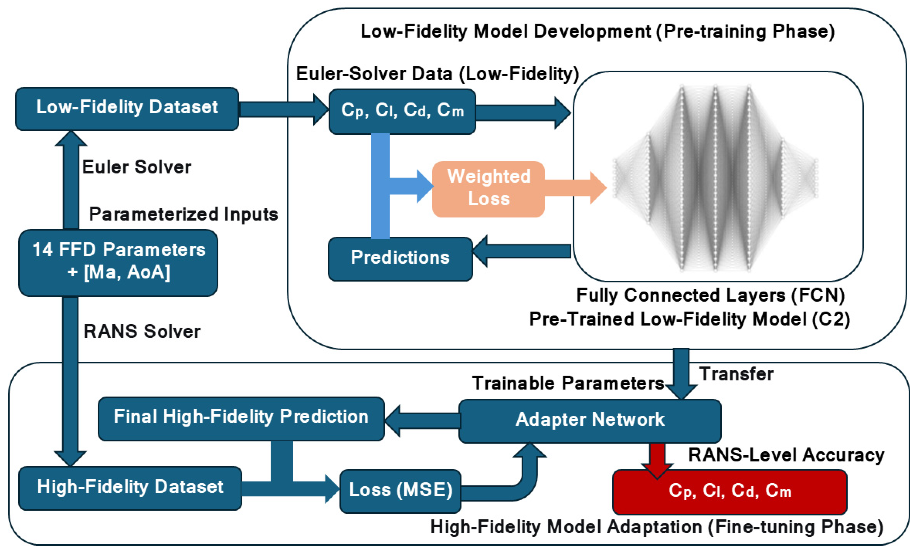
The end-to-end workflow of the proposed transfer learning framework is depicted in Figure 1. The process consists of two sequential stages: (1) the pre-training stage, where a deep neural network is trained on a large dataset of low-fidelity Euler simulations to become an accurate surrogate model (Model C2); and (2) the fine-tuning stage, where the pre-trained model is frozen and a lightweight adapter network is appended to its output. This adapter is then trained on a small set of high-fidelity RANS data to learn the residual mapping from Euler to RANS solutions. The high-fidelity RANS data, used as the target for fine-tuning, was generated offline prior to this process.
The overall workflow of the proposed multi-fidelity transfer learning framework is illustrated in Figure 1.
An iterative process was conducted to identify the most effective network architecture for mapping parameterized geometries and flow conditions to aerodynamic outputs. Initial architectures based on convolutional neural networks (CNNs) proved inadequate for this regression task, leading to poor generalization, particularly for drag prediction (see Appendix A for details). Consequently, a Fully Connected Network (FCN) architecture was adopted, which provided superior performance and became the basis for our final model.
An iterative model development process was undertaken to identify an effective network architecture. The fully connected neural network operation is defined as follows:
a j = w i , j x i + w i + 1 , j x i + 1 + b i y j = h a j
where h represents the activation function.
The ReLU activation function is employed:
ReLU x = max ( 0 , x )
Models C1 and C2 represented enhanced FCN architectures with several key improvements. Targeted data augmentation was implemented during the development of the low-fidelity Model C2 to improve performance in poorly predicted regions of the flight envelope. The procedure involved: first training an initial model on the baseline dataset; then identifying high-error samples (e.g., high RMSE in pressure distribution) on a validation set; subsequently defining localized sampling bounds around these under-performing points encompassing FFD parameters, Mach number, and angle of attack; generating new sample points within these bounds using Latin Hypercube Sampling (LHS); running new Euler simulations for these configurations; and finally adding these augmented samples to the original training dataset for retraining. This iterative strategy efficiently improved accuracy in challenging areas like transonic shock regions without the computational expense of generating a vastly larger uniform dataset. Custom normalization schemes were developed for drag and moment coefficients:
Custom normalization for drag coefficient:
C d _ t r a n s f o r m = 0.4 log C d 10,000
Custom normalization for moment coefficient:
C m y _ t r a n s f o r m = exp C m y 0.965 0.04
The Mean Squared Error loss function was modified by introducing component-specific weights:
L C = 1 n + 3 m α i = 1 n C ^ p i C p i 2 + β j = 1 m C ^ l j C l j 2 + γ k = 1 m C ^ d k C d k 2 + δ s = 1 m C ^ m y s C m y s 2
where α ,   β ,   γ ,   δ are weighting coefficients for pressure distribution, lift coefficient, drag coefficient, and moment coefficient, respectively.
The final C2 model, an optimized FCN, was established as the robust low-fidelity predictor, capable of accurately mapping geometric and flow parameters to Euler-based aerodynamic outputs.

2.2.2. Evaluation Metrics

The model performance was evaluated using the following metrics:
Root Mean Square Error for pressure distribution:
R M S E x = 1 n i = 1 n C ^ p i C p i 2
Coefficient of determination for force coefficients:
R 2 = 1 i y ^ i y i i y ¯ i y i

2.2.3. Transfer Learning for High-Fidelity Prediction

To achieve high-fidelity predictions with minimal data, a transfer learning strategy was employed. This involved freezing the parameters of the pre-trained low-fidelity model (C2) and appending a separate, trainable fully connected network (FCN) module to its output. This adapter network learns the residual mapping from the Euler-based predictions to the target RANS data.
The transfer learning framework is formulated as follows:
y R A N S = f p r e - t r a i n e d ( x ) + f a d a p t e r ( f p r e - t r a i n e d ( x ) )
where f p r e - t r a i n e d represents the frozen pre-trained model on Euler data, and f a d a p t e r is the trainable adapter network that learns the residual mapping to RANS data.
The training objective is:
min θ a d a p t e r y R A N S f p r e - t r a i n e d ( x ) + f a d a p t e r ( f p r e - t r a i n e d ( x ) ; θ a d a p t e r ) 2
where θ a d a p t e r denotes the parameters of the adapter network. The definitions of the selected symbols can be found in Table 1.
During training, only the parameters of the appended adapter network were updated using the limited RANS dataset. This approach allows the model to learn the correction required to shift from Euler to RANS results without distorting the underlying aerodynamic relationships learned from the abundant low-fidelity data.
This transfer learning framework was successfully applied for fidelity enhancement and was extended to accomplish simultaneous fidelity and flight condition transfer, as well as fidelity and geometric shape transfer, demonstrating the versatility of the proposed methodology.

3. Results

3.1. Performance of Low-Fidelity Predictive Models

The iterative development process yielded a key insight: for mapping parameterized geometries and flight conditions to aerodynamic coefficients, a well-tuned Fully Connected Network (FCN) is markedly more effective and efficient than a more complex Convolutional Neural Network (CNN). This led to the selection of an FCN as the optimal architecture (see Appendix A.1 for the comparative evolution of models). The final low-fidelity model, designated C2, incorporated targeted enhancements that significantly boosted its predictive accuracy, as detailed below.
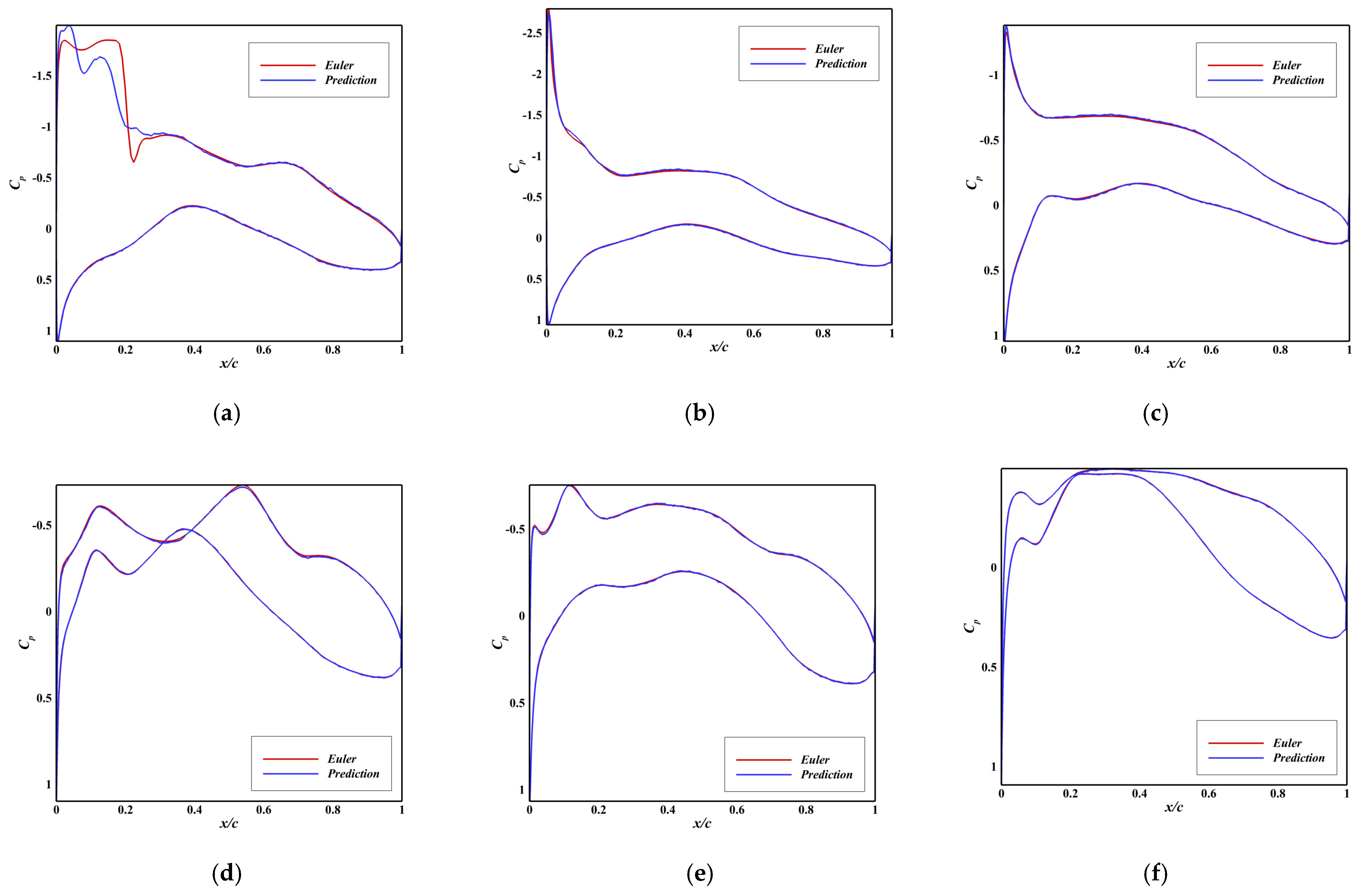
The culmination of the development process was Model C2, an enhanced FCN. Its performance, summarized in Figure 2 and Table 2, represents a robust predictive capability for low-fidelity data.
Pressure Distribution Prediction: Model C2 accurately captures the Cp distribution across most of the test cases. For over 75% of the test samples, the predictions are virtually indistinguishable from the Euler solutions, with RMSE values primarily in the order of 10−2 (e.g., Figure 2e,f: RMSE of 0.055 and 0.041). The primary source of error remains the prediction of shock location and strength in transonic regimes (e.g., Figure 2a: RMSE of 0.201 at Ma = 0.63, AoA = 3.55°), a known challenge for inviscid Euler methods themselves.
The model exhibits exceptional predictive accuracy for the force coefficients. For the lift coefficient (Cl), an R2 value of 0.999 combined with 99.2% of predictions falling within a 5% relative error (Table 3, Table 4, Table 5 and Table 6) indicates a near-perfect correlation. Similarly, the drag coefficient (Cd) is predicted with remarkably high accuracy, achieving an R2 of 0.938. More significantly, 90.7% of the Cd predictions have an absolute error of less than 1 count (0.0001), and 91.5% are within a 5% relative error bracket—a notable achievement for a parameter notoriously difficult to predict, attributable directly to the custom logarithmic normalization scheme (Equation (16)). In the case of the moment coefficient (Cm), the R2 value of 0.998 reflects excellent correlation; however, the relative error performance is lower, with 68.7% of predictions within a 5% relative error. This discrepancy arises from the very small magnitude of Cm values, where minor absolute errors result in large relative deviations. The targeted weighting applied in the loss function (Equation (12)) successfully mitigated this issue, yielding significant improvements over previous models.
The success of Model C2 confirms that a meticulously designed FCN, empowered by targeted data sampling, problem-specific normalization, and a weighted loss function, can serve as a highly accurate and extremely fast surrogate (0.317 s for 300 predictions) for low-fidelity aerodynamic analysis.

3.2. Performance of High-Fidelity Transfer Learning Models

3.2.1. Fidelity Transfer (Euler to RANS)

The pre-training and fine-tuning strategy was first applied to learn the mapping from low-fidelity (Euler) to high-fidelity (RANS) data for the same range of geometries and flight conditions.
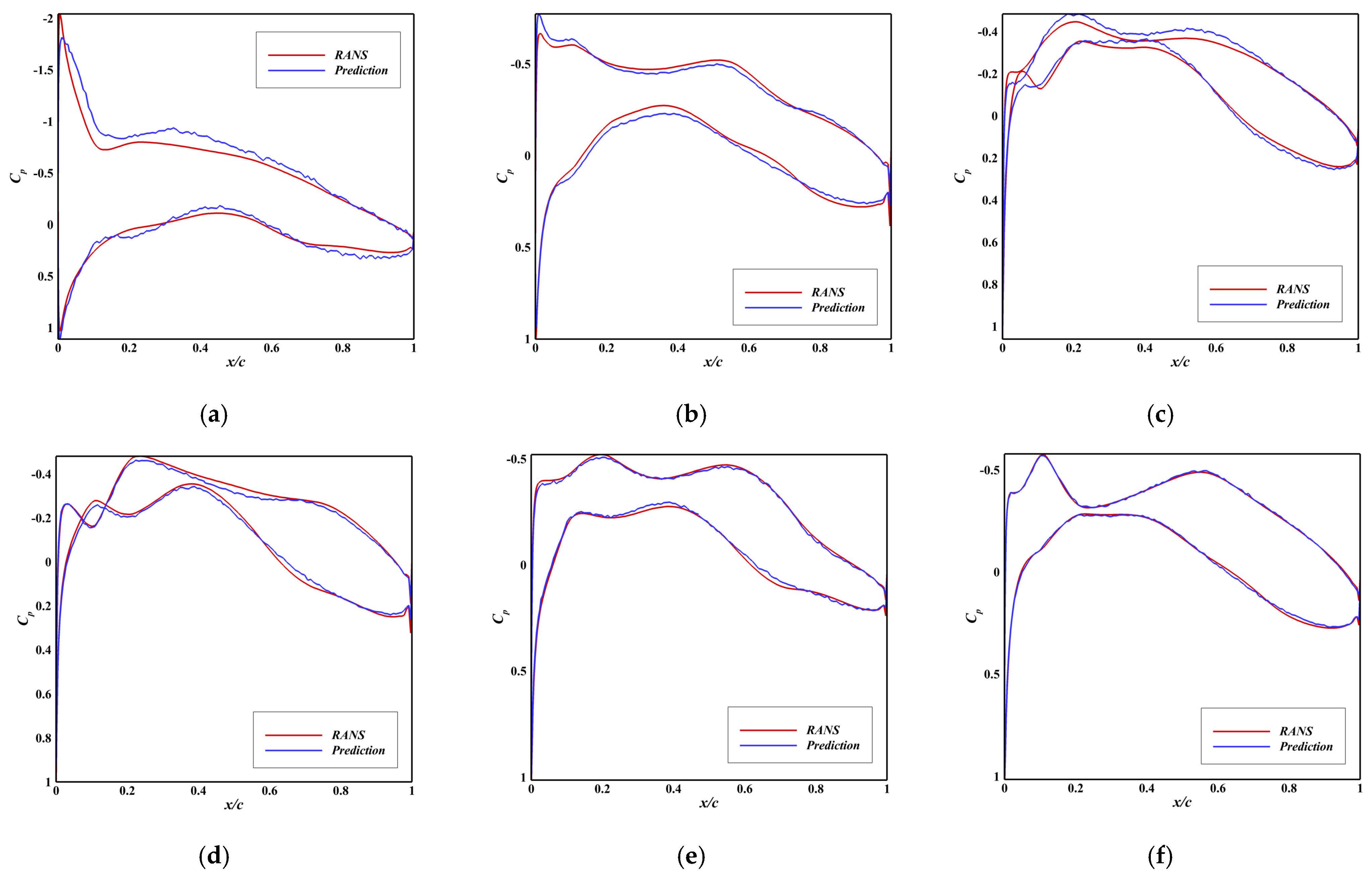
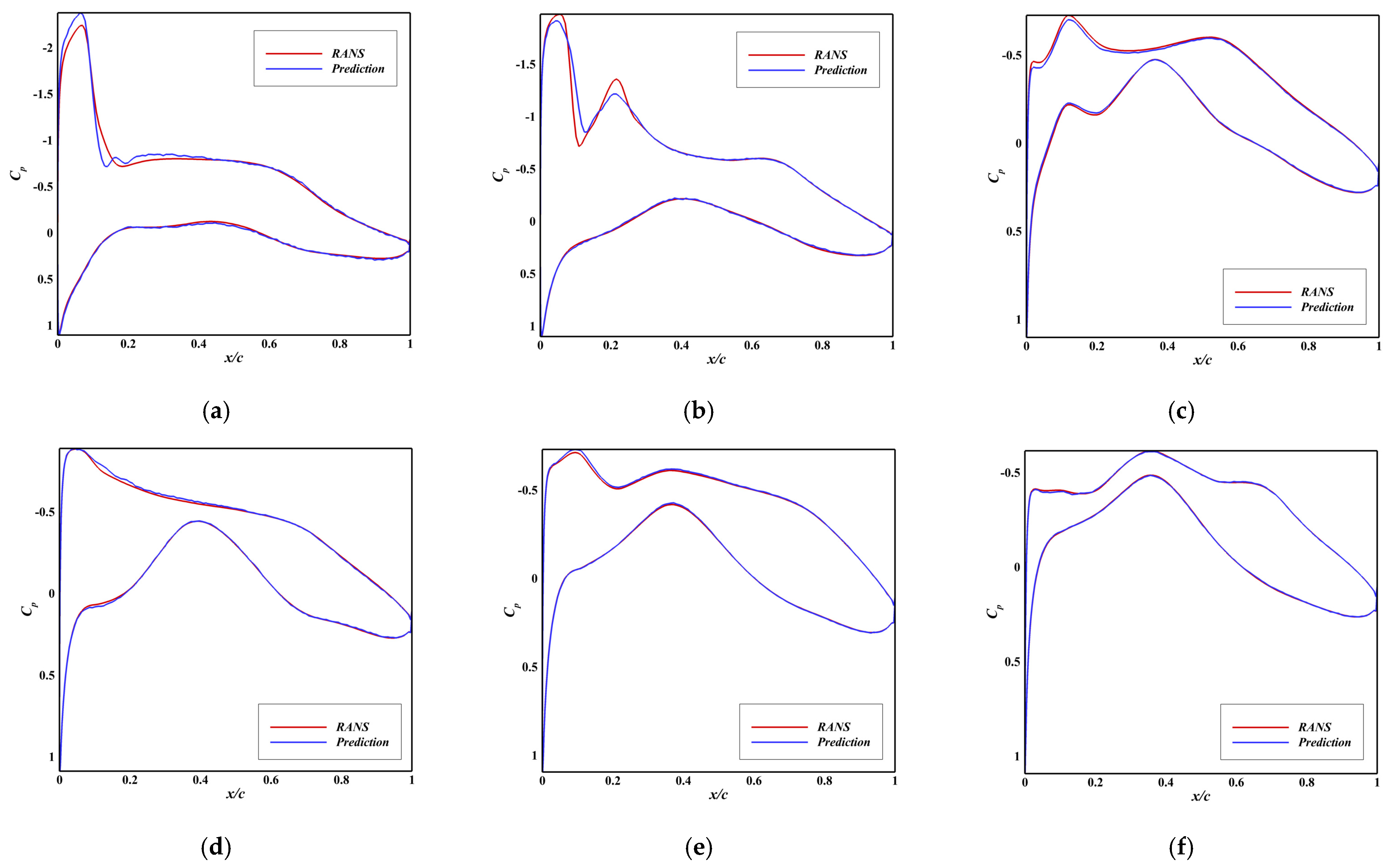
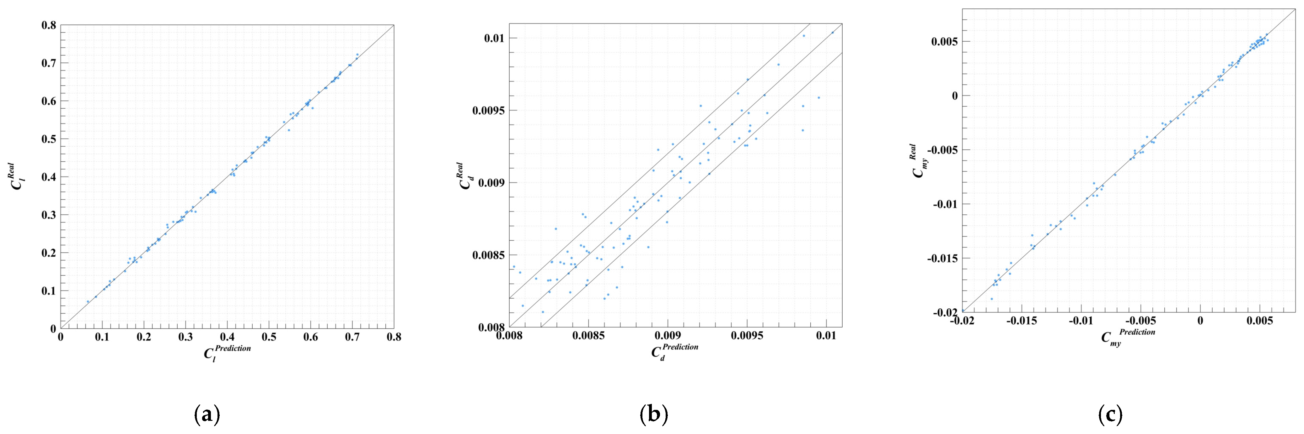
The D1 model (Ma ∈ [0.4, 0.6]), trained on only 700 RANS samples, successfully captured the RANS pressure distributions (Figure 3). The predictions for Cl (R2 = 0.999) and Cm (R2 = 0.999) were excellent. While the Cd predictions in Figure 4b appear scattered, the vast majority (83%) lie within an absolute error of 2 counts, a highly respectable accuracy given the small dataset and the complexity of predicting viscous drag (Table 3).
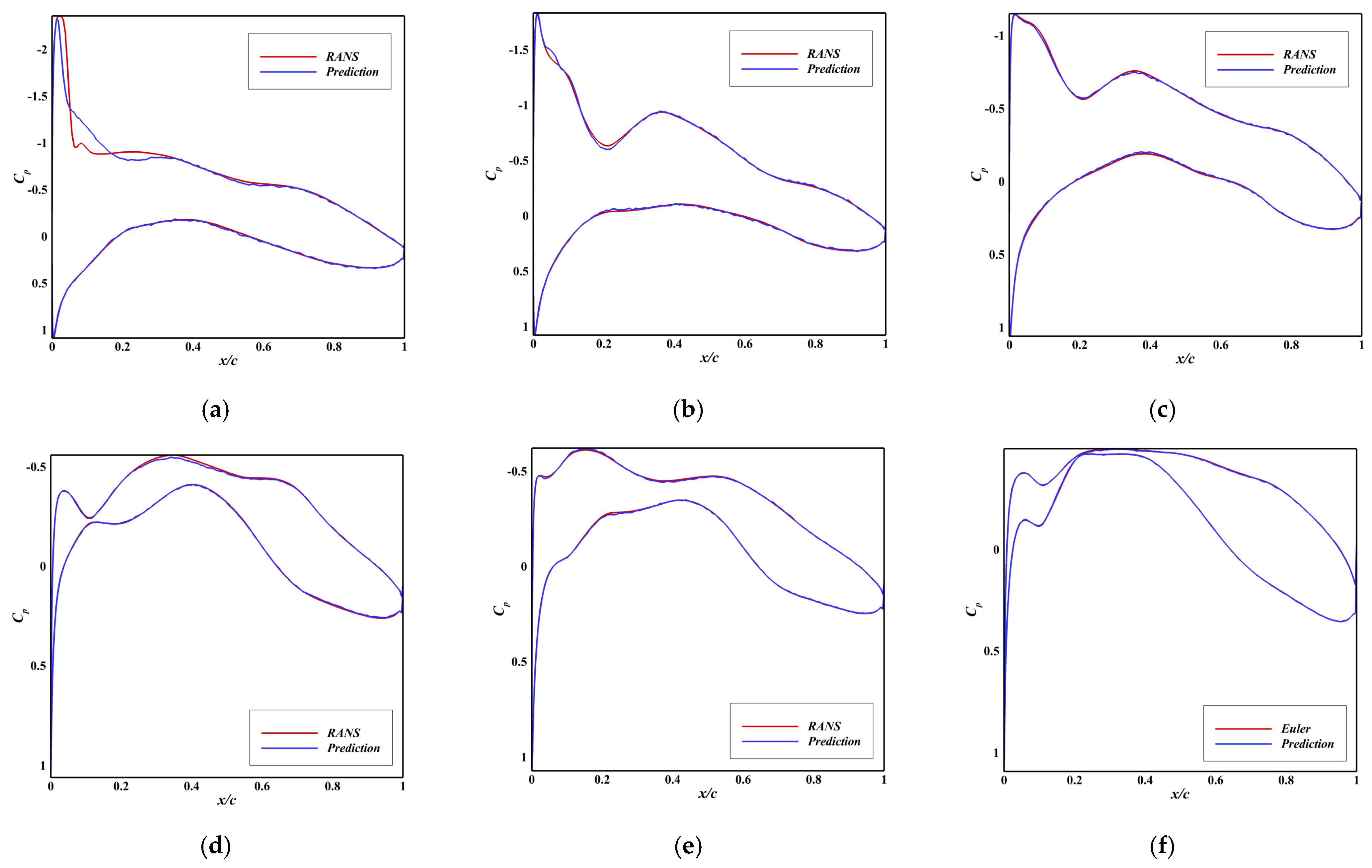
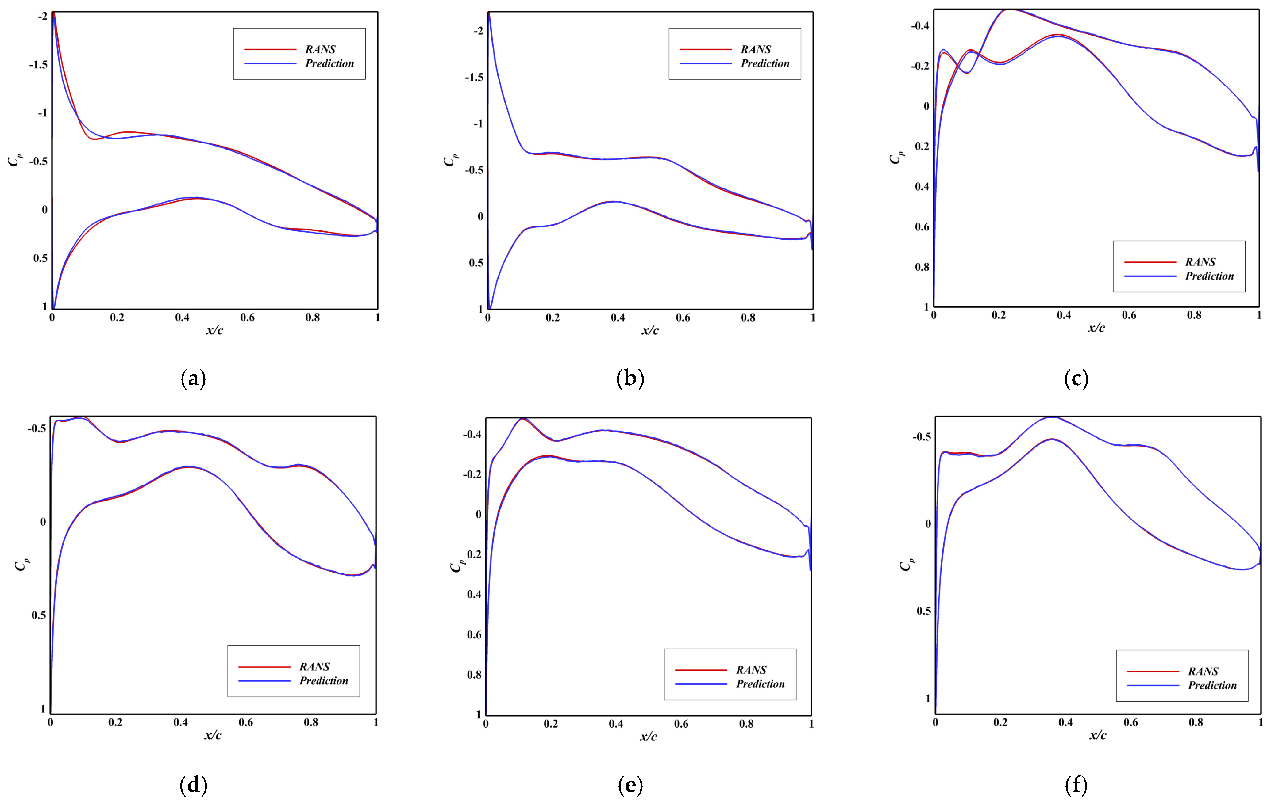
The D2 model (Ma ∈ [0.6, 0.65]) addressed the more challenging transonic regime. Despite the increased physical complexity, it maintained strong performance for Cp, Cl, and Cm (Figure 5 and Figure 6a,c). The prediction of Cd in this regime is more difficult, yet the model achieved an R2 of 0.947, with 99% of predictions within a 10% relative error (Table 4).
An ablation study confirmed the necessity of pre-training; a model (D’) trained from scratch on the same RANS data failed completely due to severe overfitting (see Appendix A.2 for details).
The dramatic reduction in overfitting achieved by our transfer learning approach, as starkly evidenced by the failure of the from-scratch model (D’), can be attributed to the powerful regularization effect of pre-training. The model pre-trained on abundant low-fidelity data has already learned a robust mapping from geometric and flow parameters to the fundamental aerodynamic relationships (e.g., the nonlinear dependence of lift on angle of attack, the general form of pressure distributions). This pre-trained model encapsulates a strong ‘physical prior’.
During fine-tuning, by freezing this pre-trained backbone and only training a small adapter network, we severely constrain the hypothesis space of the model. The adapter network does not need to learn aerodynamics from scratch; it only needs to learn the consistent residual or correction between the low-fidelity (inviscid) and high-fidelity (viscous) solutions. This is a much simpler and more constrained task. In contrast, training a model from scratch on limited high-fidelity data must simultaneously learn both the underlying aerodynamics and the high-fidelity effects, making it highly susceptible to memorizing noise and overfitting, as seen with Model D’.

3.2.2. Combined Fidelity and Condition Transfer (Ma Range Extension)

The transfer learning framework was further challenged to generalize to both a new fidelity (RANS) and a new flight condition (Ma ∈ [0.1, 0.4]). To accomplish this, a direct transfer approach was employed, fine-tuning the original pre-trained model (on Ma ∈ [0.4, 0.65], Euler) directly on the new target domain (Ma ∈ [0.1, 0.4], RANS).
The E2 model, utilizing this strategy with only 300 samples, was highly successful. It accurately predicted pressure distributions (Figure 7) and force coefficients (Figure 8, Table 5). The revised E2 model, with 500 samples and further tuned loss weights, enhanced the moment coefficient prediction (65% within 5% error, Table 6). This successful direct approach stands in clear contrast to a sequential transfer strategy, which proved ineffective for this task (see Appendix A.3, Model E1). These results collectively demonstrate that the pre-trained model learns fundamental aerodynamic relationships that are transferable across Mach numbers, and that direct transfer is a more robust and effective strategy for simultaneous fidelity and condition adaptation.
This superiority of the direct transfer strategy can be explained by considering the optimization landscape. The two-step process (E1) first fine-tunes the model on a new condition within the same fidelity domain (low-fidelity Euler data at low Mach). This specialization likely drives the model’s parameters into a region of the weight space that is highly optimized for low-fidelity predictions in that new condition, but potentially entrenches the biases inherent to the Euler equations.
Subsequently, attempting a second transfer to learn the fidelity correction (to RANS) from this specialized state becomes difficult. The model may be ‘trapped’ in a local minima suited for Euler physics, making it intractable to learn the additional, often contradictory, physical effects (e.g., viscosity, turbulence) required for RANS.
In contrast, the direct approach (E2) fine-tunes the original pre-trained model (which possesses general aerodynamic knowledge across the original Mach range) directly on the combined new target: the new condition and the new fidelity. This allows the adapter network to simultaneously learn the corrections for both the shift in flow condition and the shift in fidelity in a coupled manner, which appears to be a more feasible and stable optimization problem.

3.2.3. Combined Fidelity and Geometry Transfer (Shape Range Extension)

Finally, the framework was tested on geometries outside the original training distribution by increasing the FFD perturbation range by 30%.
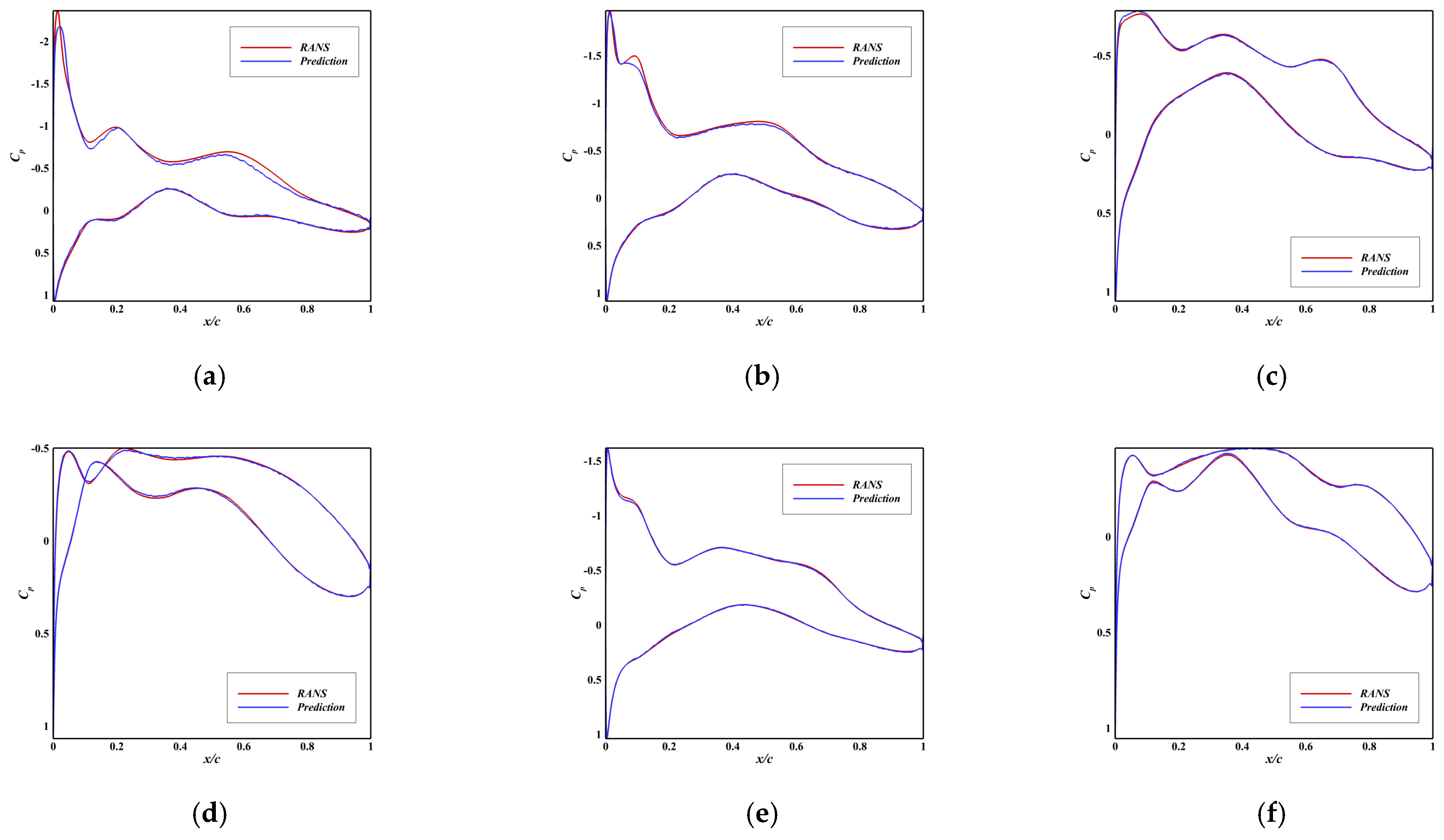
The G1 model (Ma ∈ [0.4, 0.6]) successfully adapted to the new geometric domain, delivering accurate predictions for Cp (Figure 9) and force coefficients (Figure 10, Table 7). The G2 model (Ma ∈ [0.6, 0.65]) faced greater difficulty due to the higher sensitivity of transonic flows to geometry changes. While its performance metrics (Table 8) are lower than G1’s, they remain strong (e.g., 87% of Cd predictions within 5% error), proving the resilience and generalizability of the transfer learning approach.

4. Discussion

The results firmly establish that a transfer learning strategy based on pre-training on low-fidelity data and fine-tuning on a small set of high-fidelity data is not only viable but highly effective for constructing aerodynamic surrogates. The key to success lies in a three-step process: (1) building a highly accurate low-fidelity predictor through careful architecture selection and data processing, (2) freezing this model to preserve learned aerodynamic knowledge, and (3) training a simple adapter network to learn the consistent difference between the low- and high-fidelity solutions.
A cross-model analysis of the force coefficient error percentages (Table 2, Table 3, Table 4, Table 7 and Table 8 conclusively demonstrates the efficacy of our novel normalization and transfer learning (TL) strategy. The evolution from the initial, failed attempts to predict drag (Cd) in Models A and B (Appendix A) to the robust performance of the low-fidelity Model C2 (91.5% of Cd predictions within 5% error) underscores the critical importance of the custom logarithmic normalization. This approach successfully eliminated the model’s inherent bias towards higher-magnitude coefficients like lift (Cl), which consistently achieved near-perfect accuracy (>99% within 5% error) across all final models.
The TL framework successfully translated this low-fidelity accuracy to the high-fidelity domain. While predicting viscous drag from inviscid data presents a greater challenge—resulting in a slight, expected dip in Cd metrics for models like D1 and D2 compared to C2—the performance remains exceptional for a data-driven surrogate (e.g., 83% of predictions within 2 counts for D1). The strong results on unseen conditions (E2) and geometries (G1, G2) further confirm that the pre-trained model encodes a generalizable aerodynamic mapping. The stark failure of the ablated models D’ and E1 (Appendix A.2 and Appendix A.3), which lacked proper pre-training or used an inferior transfer strategy, provides compelling counterevidence that our end-to-end approach is not merely beneficial but essential for achieving high-fidelity accuracy with limited data.
The framework’s ability to simultaneously transfer across fidelity and either flight conditions or geometric perturbations is its most powerful feature. It demonstrates that the low-fidelity model encapsulates a general understanding of aerodynamics that is not tightly coupled to a specific Mach number or shape domain. This makes the method particularly valuable for engineering design and optimization, where quick exploration of new design spaces with high-fidelity accuracy is required.
Nevertheless, the current validation is primarily limited to RAE2822-derived geometries and Mach ranges between 0.1 and 0.65. While these conditions are representative of many subsonic and transonic applications, they do not cover a broader spectrum of aerodynamic configurations. To further strengthen the generalizability of the proposed framework, future work will extend validation to other airfoil families, such as the widely used NACA series, and incorporate comparisons with experimental datasets. Such efforts will provide a more comprehensive assessment of the model’s robustness across diverse aerodynamic regimes and practical scenarios.
Furthermore, we address the potential risk of negative transfer, wherein pre-training on the source domain (Euler data) could potentially hinder learning in the target domain (RANS). In our experiments, no such phenomenon was observed. We attribute this to the strong physical consistency between the Euler and RANS frameworks; the inviscid Euler equations effectively capture the dominant pressure distribution and wave dynamics, which form a reliable prior for the more complex viscous flows. The architectural choice of freezing the pre-trained model and solely training a small adapter network was pivotal. This design forces the model to learn only the residual, fidelity-specific corrections (primarily viscous effects) rather than attempting to re-learn the underlying aerodynamics from a potentially misleading low-fidelity basis. This approach effectively mitigates the risk of negative transfer by constraining the hypothesis space and building upon a physically meaningful foundation. However, we acknowledge that negative transfer could become a concern if the low-fidelity model is poorly constructed or if the physical gap between the source and target domains is too large, an area worthy of further investigation.
The primary limitation remains the prediction of strong shock waves in transonic flows, a challenge inherent to the underlying Euler and RANS models themselves. Future work could explore incorporating physical constraints or using higher-fidelity data (e.g., DDES) in the transfer learning process to improve performance in these critical regimes.
It is also important to note that the demonstrated generalizability of the framework, while successful within the tested Mach number and geometric perturbation ranges, has its boundaries. The model’s performance on flow regimes far outside those presented (e.g., hypersonic flows or deep stall conditions) or on fundamentally different airfoil families remains untested and constitutes an important area for future investigation. Extending the framework to a broader spectrum of operating conditions and geometric shapes will be a key focus of subsequent research.

5. Conclusions

This study has successfully developed and validated a transfer-learning-based framework for efficient and accurate aerodynamic prediction, demonstrating a significant potential to reduce computational costs in the aerodynamic design and optimization of 2D airfoils, a critical component of wing design. The core achievement lies in establishing a robust pipeline that leverages low-fidelity Euler data to enable high-fidelity RANS predictions with minimal computational expense.
This research proceeded through four key phases. First, a comprehensive dataset was generated using FFD parameterization of the RAE2822 airfoil and Latin Hypercube Sampling across geometric and flow parameters. Second, an intensive model development process yielded the optimal low-fidelity predictor (C2 model), a fully connected network that achieved exceptional accuracy on Euler data (R2 > 0.999 for Cl, R2 = 0.938 for Cd, and RMSE as low as 0.041 for pressure distributions). Third, a novel pre-training and fine-tuning transfer learning strategy was implemented, whereby the pre-trained C2 model was frozen and coupled with a trainable adapter network. This approach successfully translated Euler-based knowledge to RANS predictions, producing high-fidelity models (D1, D2) with only 700 samples per Mach regime. Finally, the framework’s versatility was proven by its extension to simultaneous fidelity-condition transfer (E2 model, Ma ∈ [0.1, 0.4]) and fidelity-geometry transfer (G1, G2 models, with +30% FFD perturbation), achieving R2 values consistently above 0.9 for force coefficients in new domains.
The results conclusively demonstrate that transfer learning is not only feasible but highly effective for aerodynamic prediction. It overcomes the fundamental limitation of traditional neural networks—poor generalization beyond their training data—by leveraging underlying physical principles learned from abundant low-fidelity data. The proposed method provides a practical pathway for rapid aerodynamic evaluation with near-RANS accuracy at a fraction of the computational cost, offering considerable promise for streamlining the initial airfoil selection and design process.
It is important to note that the present work is rigorously validated only for 2D airfoils. The extension of this framework to three-dimensional configurations, which involves significantly greater complexity in flow structures and geometric parameterization, represents a primary objective for future research.
Despite its strong performance, the current framework exhibits limitations that chart a course for future work. The primary constraint lies in predicting strong shock waves and their interaction with boundary layers in transonic regimes, a challenge inherent to the underlying RANS models themselves. This could be addressed by incorporating higher-fidelity data sources, such as Detached Eddy Simulation (DES) or scale-resolving simulations, into the transfer learning process, even if only for a small subset of critical cases. Furthermore, while the model generalizes well to new geometries within a parameterized family, its performance on fundamentally different airfoil shapes (e.g., from a different design family) remains an open question. Future investigations will explore the use of coarse-grid RANS solutions as a more physically consistent low-fidelity source, validate the model on full aerodynamic polar predictions for optimization workflows, and ultimately extend the framework to three-dimensional configurations, which represent the ultimate test of its scalability and practical engineering value.
Additionally, validation will be broadened to include different airfoil families (e.g., NACA) and experimental measurements, thereby ensuring wider applicability of the framework. Future work will focus on improving shock wave prediction, exploring coarse-grid RANS as a more consistent low-fidelity source, validating the model on full polar predictions for engineering optimization, and ultimately extending the framework to complex three-dimensional configurations.

Author Contributions

Conceptualization, Y.H. and B.W.; methodology, Y.H. and X.C.; software, Y.H.; validation, Y.H. and Y.W.; formal analysis, Y.H. and Q.J.; investigation, Y.H.; resources, Y.H. and Z.Z.; data curation, Y.H. and M.Z.; writing—original draft preparation, Y.H.; writing—review and editing, Y.H. and X.M.; visualization, Y.H. and X.C.; supervision, B.W.; project administration, X.M.; funding acquisition, B.W. All authors have read and agreed to the published version of the manuscript.

Funding

This research received no external funding.

Data Availability Statement

The datasets generated and analyzed during this study are available from the corresponding author upon reasonable request for academic and research purposes.

Conflicts of Interest

The authors declare no conflicts of interest.

Appendix A

Appendix A.1. Preliminary Model Development (Model A/B/C)

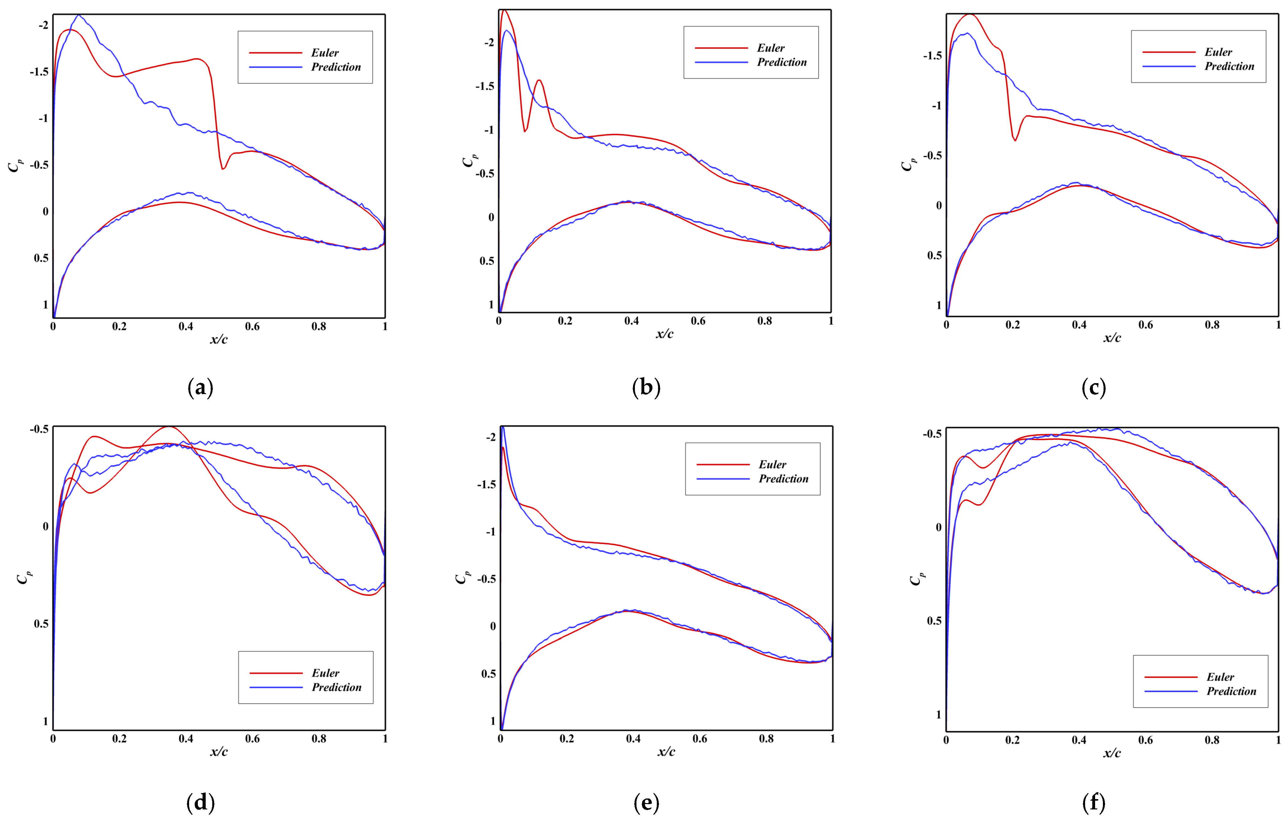
The initial Model A, which utilized a Convolutional Neural Network (CNN) operating on 290 airfoil coordinate points, demonstrated unsatisfactory performance. As shown in Figure A1, the predicted pressure distributions (Cp) exhibited considerable deviation from the Euler solutions, with Root Mean Square Error (RMSE) values consistently around 0.2–0.35. More critically, its predictive capability for force coefficients was virtually non-existent for drag (Cd) and moment (Cm), with R2 values of −6.568 and 0.331, respectively (Figure A2, Table A1). This failure underscored that CNNs, while powerful for image-like data, are not inherently suitable for this structured parameter-to-parameter regression task and can lead to severe overfitting with limited data.
Figure A1. Comparison between Predicted and Ground Truth Pressure Distributions of Model A. (a) RMSE = 0.345, Ma = 0.68, AoA = 3.6°; (b) RMSE = 0.279, Ma = 0.61, AoA = 3.6°; (c) RMSE = 0.253, Ma = 0.66, AoA = 3.0°; (d) RMSE = 0.229, Ma = 0.47, AoA = 1.0°; (e) RMSE = 0.207, Ma = 0.53, AoA = 3.2°; (f) RMSE = 0.168, Ma = 0.62, AoA = 0.5°.
Applsci 15 10820 g0a1
Figure A2. Scatter Plot of Force Coefficient Correlation for Model A. (a) Correlation Diagram for Lift Coefficient, R2 = 0.963. (b) Correlation Diagram for Drag Coefficient, R2 = −6.568. (c) Correlation Diagram for Moment Coefficient, R2 = 0.331.
Applsci 15 10820 g0a2
Table A1. Table of Force Coefficient Contributions for Model A.
Percentage of Force Coefficients for Model A
Percentage of Lift Coefficient Predictions with <5% Error39%
Percentage of Lift Coefficient Predictions with <10% Error67%
Percentage of Lift Coefficient Predictions with <20% Error93%
Percentage of Drag Coefficient Predictions with <5% Error0%
Percentage of Drag Coefficient Predictions with <10% Error0%
Percentage of Drag Coefficient Predictions with <20% Error0%
Percentage of Moment Coefficient Predictions with <5% Error1%
Percentage of Moment Coefficient Predictions with <10% Error4%
Percentage of Moment Coefficient Predictions with <20% Error7%
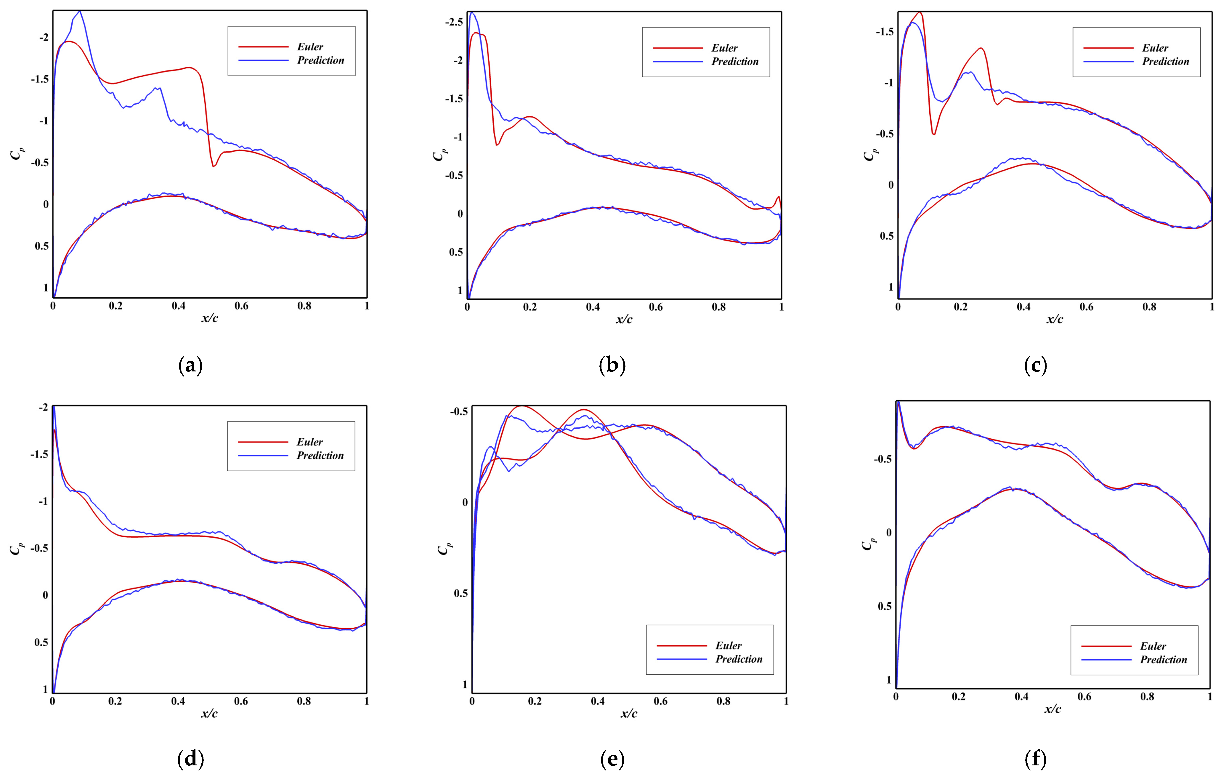
Model B addressed the input dimensionality by using the 14 original FFD parameters instead of the 290 coordinates. This change, coupled with max-value normalization, led to a marked improvement. As evidenced in Figure A3, the predicted pressure distributions showed better agreement with the Euler solutions compared to Model A, though significant errors remained (RMSE ~0.1–0.3). The correlation for force coefficients also improved substantially, with lift coefficient (Cl) and moment coefficient (Cm) achieving strong correlations (R2 > 0.98), as shown in Figure A4. However, the model still failed to learn an accurate mapping for the drag coefficient (R2 = 0.621). These results indicated that while simplifying the input was beneficial, the CNN-based feature extraction remained a limiting factor, particularly for capturing the complex relationships underlying drag prediction and detailed pressure distribution.
Figure A3. Comparison between Predicted and Ground Truth Pressure Distributions of Model B. (a) RMSE = 0.298, Ma = 0.68, AoA = 3.6°; (b) RMSE = 0.241, Ma = 0.59, AoA = 4.0°; (c) RMSE = 0.212, Ma = 0.65, AoA = 2.2°; (d) RMSE = 0.181, Ma = 0.42, AoA = 2.8°; (e) RMSE = 0.157, Ma = 0.49, AoA = −0.5°; (f) RMSE = 0.114, Ma = 0.62, AoA = 0.5°.
Applsci 15 10820 g0a3
Figure A4. Scatter Plot of Force Coefficient Correlation for Model B. (a) Correlation Diagram for Lift Coefficient, R2 = 0.986. (b) Correlation Diagram for Drag Coefficient, R2 = 0.621. (c) Correlation Diagram for Moment Coefficient, R2 = 0.993.
Applsci 15 10820 g0a4
The consistently poor performance of the CNN-based architectures (Models A and B), particularly in predicting the drag coefficient (Cd), can be primarily attributed to a mismatch between the inductive biases of CNNs and the nature of our regression task. CNNs excel at learning translation-invariant features from grid-like, spatially correlated data (e.g., images). However, our task fundamentally involves mapping a low-dimensional parameter vector (14 FFD parameters + 2 flow conditions) to another low-dimensional vector of aerodynamic coefficients. This is a global parameter-to-parameter mapping problem rather than a feature detection problem on a spatial field.
The failure of Model A, which used raw coordinate points, suggests that presenting the geometry as a pseudo-‘image’ did not provide a meaningful spatial structure for the CNN to exploit. The improvement seen in Model B, which used the original FFD parameters, further supports this. It indicates that the critical information was contained within the parameter space itself, not in its spatial representation. The CNN’s complex feature extraction layers applied to this structured tabular data likely led to overfitting and an inability to learn the precise nonlinear relationships governing drag, which is highly sensitive to subtle changes in geometry and flow.
Therefore, we conclude that the suboptimal performance is inherent to the architecture’s bias, not merely due to data scarcity. A simpler Fully Connected Network, which is inherently more suited for learning global mappings between dense vectors, proved to be a far more effective and efficient choice for this task.
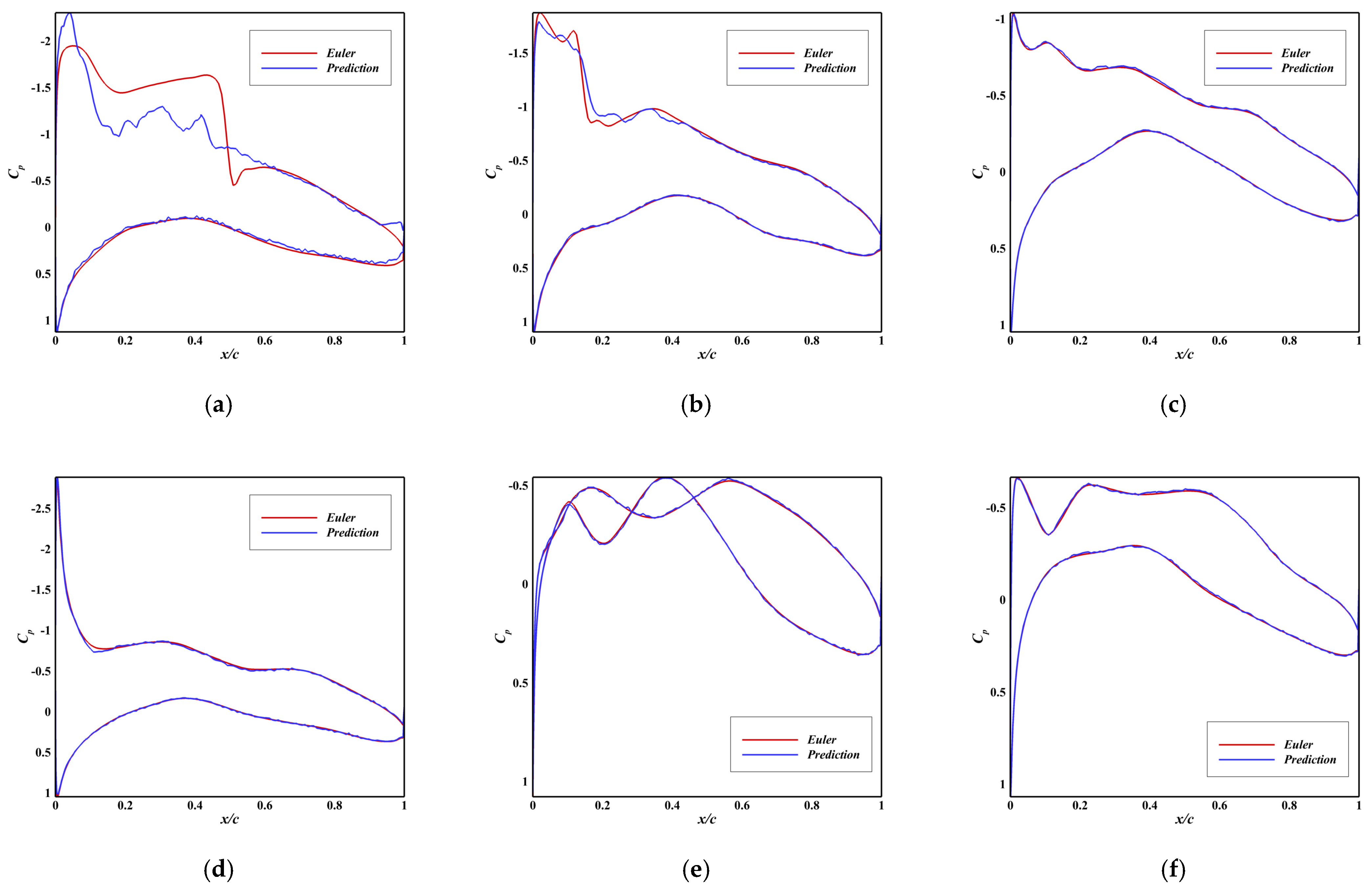
Model C adopted a purely Fully Connected Network (FCN) architecture. This simpler architecture, operating on the 14 FFD parameters and 2 flow conditions, yielded superior performance for pressure distribution prediction while maintaining comparable accuracy for force coefficients compared to Model B.
Model C adopted a simplified feature extraction backbone comprising only two 1D convolutional layers, followed by an eight-layer fully connected network. The first convolutional layer utilized 5 filters with a kernel size of 5, while the second layer employed 10 filters with a kernel size of 2; both were followed by 2 × 1 max pooling and ReLU activation. The resulting feature vector was flattened into 72 elements and processed by the FCN, which consisted of successive layers with 1024, 2048, 2048, 2048, 2048, and 586 ReLU-activated neurons, culminating in a linear output layer of 293 neurons. This architecture differed from Model B solely in the reduction in convolutional layers, retaining an identical FCN structure.
Figure A5. Comparison between Predicted and Ground Truth Pressure Distributions of Model C. (a) RMSE = 0.373, Ma = 0.68, AoA = 3.6°; (b) RMSE = 0.214, Ma = 0.63, AoA = 3.3°; (c) RMSE = 0.141, Ma = 0.44, AoA = 2.1°; (d) RMSE = 0.119, Ma = 0.46, AoA = 3.4°; (e) RMSE = 0.103, Ma = 0.58, AoA = −0.9°; (f) RMSE = 0.069, Ma = 0.55, AoA = 0.7°.
Applsci 15 10820 g0a5

Appendix A.2. Ablation Study on the Necessity of Pre-Training (Model D’)

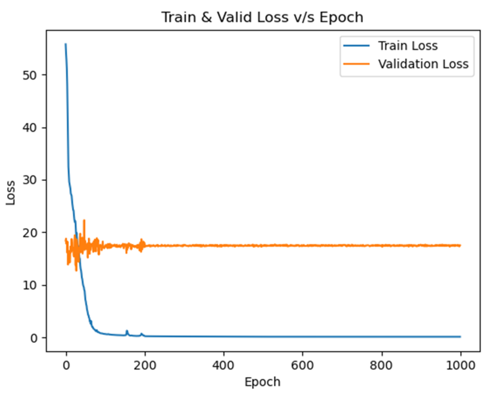
Crucially, the ablation study using the D’ model confirmed the necessity of the pre-trained model. When trained from scratch on the same 700 RANS samples without transfer learning, the D’ model failed completely, exhibiting severe overfitting, nonsensical force coefficient predictions (R2_{Cd} = −159.6, Figure A6), and no predictive capability (Table A2). This stark contrast undeniably proves that the knowledge embedded in the low-fidelity model is essential for achieving high accuracy with very limited high-fidelity data.
Figure A6. Convergence Curve of the Loss Function for Model D’.
Applsci 15 10820 g0a6
Table A2. Table of Force Coefficient Contributions for Model D’.
Percentage of Force Coefficients for Model D’
Percentage of Lift Coefficient Predictions with <1% Error16%
Percentage of Lift Coefficient Predictions with <5% Error71%
Percentage of Lift Coefficient Predictions with <10% Error91%
Percentage of Drag Coefficient Predictions within an Absolute Error of 1 Count0%
Percentage of Drag Coefficient Predictions within an Absolute Error of 2 Counts0%
Percentage of Drag Coefficient Predictions with <5% Error0%
Percentage of Drag Coefficient Predictions with <10% Error0%
Percentage of Drag Coefficient Predictions with <20% Error0%
Percentage of Moment Coefficient Predictions with <5% Error0%
Percentage of Moment Coefficient Predictions with <10% Error0%
Percentage of Moment Coefficient Predictions with <20% Error0%

Appendix A.3. Results of the Two-Step Transfer Strategy (Model E1)

The initial attempt with the E1 model, which employed a two-step transfer (first Operating Condition, then fidelity), failed (Figure A7 and Figure A8, Table A3). This suggests that the model became overly specialized to Euler physics in the first step, making subsequent correction to RANS intractable.
Figure A7. Comparison between Predicted and Ground Truth Pressure Distributions of Model E1. (a) RMSE = 0.281, Ma = 0.39, AoA = 3.8°; (b) RMSE = 0.187, Ma = 0.11, AoA = 1.3°; (c) RMSE = 0.163, Ma = 0.39, AoA = −0.2°; (d) RMSE = 0.139, Ma = 0.15, AoA = −0.4°; (e) RMSE = 0.115, Ma = 0.26, AoA = 0.7°; (f) RMSE = 0.089, Ma = 0.27, AoA = 0.3°.
Applsci 15 10820 g0a7
Figure A8. Scatter Plot of Force Coefficient Correlation for Model E1. (a) Correlation Diagram for Lift Coefficient, R2 = 0.973. (b) Correlation Diagram for Drag Coefficient, R2 = −11.3. (c) Correlation Diagram for Moment Coefficient, R2 = 0.932.
Applsci 15 10820 g0a8
Table A3. Table of Force Coefficient Contributions for Model E1.
Percentage of Force Coefficients for Model E1
Percentage of Lift Coefficient Predictions with <1% Error11%
Percentage of Lift Coefficient Predictions with <5% Error61%
Percentage of Lift Coefficient Predictions with <10% Error84%
Percentage of Drag Coefficient Predictions within an Absolute Error of 1 Count7%
Percentage of Drag Coefficient Predictions with <5% Error16%
Percentage of Drag Coefficient Predictions with <10% Error29%
Percentage of Drag Coefficient Predictions with <20% Error69%
Percentage of Moment Coefficient Predictions with <5% Error5%
Percentage of Moment Coefficient Predictions with <10% Error19%
Percentage of Moment Coefficient Predictions with <20% Error37%

References

  1. Szczepaniak, R.; Czyż, Z.; Bąbel, R.; Mańka, A.; Zahorski, T.; Omen, Ł.; Kosicka, E.; Matijosius, J.; Ngouobe, J.N. Analysis of the basic aerodynamic characteristics of an unmanned combat aerial vehicle based on a CAD model. Adv. Sci. Technol. Res. J. 2025, 19, 235–247. [Google Scholar] [CrossRef]
  2. Fertahi Sed-Dîn Rehman, S.; Benini, E.; Lahrech, K.; Samaouali, A.; Arbaoui, A.; Kadiri, I.; Agounoun, R. Insights from the Last Decade in Computational Fluid Dynamics (CFD) Design and Performance Enhancement of Darrieus Wind Turbines. Processes 2025, 13, 370. [Google Scholar] [CrossRef]
  3. Guindani, B. Data-Driven Approaches for Managing Resources of Cloud, Edge, and High-Performance Computing Systems. Ph.D. Thesis, Politecnico di Milano, Milan, Italy, 2023. [Google Scholar]
  4. Slotnick, J.P.; Khodadoust, A.; Alonso, J.; Darmofal, D.; Gropp, W.; Lurie, E.; Mavriplis, D.J. CFD Vision 2030 Study: A Path to Revolutionary Computational Aerosciences; Contractor Report (CR); NASA Langley Research Center: Hampton, VA, USA, 2014. [Google Scholar]
  5. Catalani, G.; Agarwal, S.; Bertrand, X.; Tost, F.; Bauerheim, M.; Morlier, J. Neural fields for rapid aircraft aerodynamics simulations. Sci. Rep. 2024, 14, 25496. [Google Scholar] [CrossRef] [PubMed]
  6. Wu, M.-Y.; He, X.-J.; Sun, X.-H.; Tong, T.-S.; Chen, Z.-H.; Zheng, C. Efficient aerodynamic shape optimization using transfer learning based multi-fidelity deep neural network. Phys. Fluids 2024, 36, 116109. [Google Scholar] [CrossRef]
  7. Allen, L.D.; Lim, J.W.; Haehnel, R.B.; Dettwiller, I.D. Rotor blade design framework for airfoil shape optimization with performance considerations. In Proceedings of the AIAA Scitech 2021 Forum, Virtual Event, 11–15 & 19–21 January 2021. [Google Scholar] [CrossRef]
  8. Qin, S.-H.; Yang, A.-M. Aerodynamic optimization of a coaxial rotor system using a deep learning-based multi-fidelity surrogate model. Eng. Appl. Comput. Fluid. Mech. 2025, 19, 2528120. [Google Scholar] [CrossRef]
  9. Wang, X.; Dong, Y.; Zou, S.; Zhang, L.; Deng, X. A semi-supervised framework for computational fluid dynamics prediction. Appl. Soft Comput. 2024, 154, 111422. [Google Scholar] [CrossRef]
  10. Chen, S.; Yuan, L.; Xiang, J.; Guo, S.; Xie, Y.; Lan, K.; Cheng, Y. Data-driven surrogate aerodynamic prediction model and lift optimization for the flapping wing rotor. Aerosp. Sci. Technol. 2025, 168, 110715. [Google Scholar] [CrossRef]
  11. Liao, P.; Song, W.; Du, P.; Zhao, H. Multi-fidelity convolutional neural network surrogate model for aerodynamic optimization based on transfer learning. Phys. Fluids 2021, 33, 127121. [Google Scholar] [CrossRef]
  12. Zhang, J. Research on Transfer Learning Modeling and Interactive Visualization Method for Aerodynamic Data. Ph.D. Thesis, South West University of Science and Technology, Mianyang, China, 2023. [Google Scholar]
  13. Runze, L.; Zhang, Y.; Haixin, C. Transfer learning from two-dimensional supercritical airfoils to three-dimensional transonic swept wings. Chin. J. Aeronaut. 2023, 36, 96–110. [Google Scholar]
  14. Jiang, S.; Durlofsky, L.J. Use of multifidelity training data and transfer learning for efficient construction of subsurface flow surrogate models. J. Comput. Phys. 2023, 474, 111800. [Google Scholar] [CrossRef]
  15. Stradtner, M.; Liersch, C.M.; Bekemeyer, P. An aerodynamic variable-fidelity modelling framework for a low-observable UCAV. Aerosp. Sci. Technol. 2020, 107, 106232. [Google Scholar]
  16. Guo, Z.; Li, C.; Chen, Y.; Song, L.; Li, J.; Feng, Z. Knowledge transfer accelerated turbine blade optimization via an sample-weighted variational autoencoder. Aerosp. Sci. Technol. 2024, 147, 108998. [Google Scholar] [CrossRef]
  17. Cui, J.; Li, H.; Liu, J.; Sun, W. Efficient Surrogate Modeling of Subsurface Flow in Porous Media with Multifidelity Training Data. In Progress and Challenge of Porous Media: Proceedings of the 16th Annual Meeting Conference on Porous Media; Springer: Berlin/Heidelberg, Germany, 2024; pp. 428–435. [Google Scholar]
  18. Song, D.H.; Tartakovsky, D.M. Transfer learning on multifidelity data. J. Mach. Learn. Model. Comput. 2022, 3, 31–47. [Google Scholar] [CrossRef]
Figure 1. Schematic of the end-to-end multi-fidelity transfer learning framework, comprising a pre-training phase on low-fidelity Euler data and a fine-tuning phase on high-fidelity RANS data.
Applsci 15 10820 g001
Figure 2. Comparison between Predicted and Ground Truth Pressure Distributions of Model C2. (a) RMSE = 0.201, Ma = 0.63, AoA = 3.55°; (b) RMSE = 0.114, Ma = 0.50, AoA = 3.8°; (c) RMSE = 0.082, Ma = 0.45, AoA = 2.35°; (d) RMSE = 0.066, Ma = 0.64, AoA = −0.4°; (e) RMSE = 0.055, Ma = 0.54, AoA = 0.6°; (f) RMSE = 0.041, Ma = 0.62, AoA = −0.5°.
Applsci 15 10820 g002
Figure 3. Comparison between Predicted and Ground Truth Pressure Distributions of Model D1. (a) RMSE = 0.173, Ma = 0.60, AoA = 3.4°; (b) RMSE = 0.095, Ma = 0.57, AoA = 3.3°; (c) RMSE = 0.073, Ma = 0.51, AoA = 2.3°; (d) RMSE = 0.062, Ma = 0.52, AoA = 0.0°; (e) RMSE = 0.055, Ma = 0.55, AoA = 0.8°; (f) RMSE = 0.045, Ma = 0.52, AoA = −0.3°.
Applsci 15 10820 g003
Figure 4. Scatter Plot of Force Coefficient Correlation for Model D1. (a) Correlation Diagram for Lift Coefficient, R2 = 0.999. (b) Correlation Diagram for Drag Coefficient, R2 = 0.901. (c) Correlation Diagram for Moment Coefficient, R2 = 0.999.
Applsci 15 10820 g004
Figure 5. Comparison between Predicted and Ground Truth Pressure Distributions of Model D2. (a) RMSE = 0.177, Ma = 0.635, AoA = 3.95°; (b) RMSE = 0.130, Ma = 0.635, AoA = 3.5°; (c) RMSE = 0.098, Ma = 0.645, AoA = 0.75°; (d) RMSE = 0.074, Ma = 0.61, AoA = 1.6°; (e) RMSE = 0.066, Ma = 0.605, AoA = 0.85°; (f) RMSE = 0.053, Ma = 0.62, AoA = 0.2°.
Applsci 15 10820 g005
Figure 6. Scatter Plot of Force Coefficient Correlation for Model D2. (a) Correlation Diagram for Lift Coefficient, R2 = 0.999. (b) Correlation Diagram for Drag Coefficient, R2 = 0.947. (c) Correlation Diagram for Moment Coefficient, R2 = 0.997.
Applsci 15 10820 g006
Figure 7. Comparison between Predicted and Ground Truth Pressure Distributions of Model E2. (a) RMSE = 0.146, Ma = 0.36, AoA = 3.5°; (b) RMSE = 0.099, Ma = 0.11, AoA = 4.0°; (c) RMSE = 0.089, Ma = 0.35, AoA = 3.9°; (d) RMSE = 0.080, Ma = 0.18, AoA = 0.6°; (e) RMSE = 0.069, Ma = 0.29, AoA = 2.2°; (f) RMSE = 0.056, Ma = 0.23, AoA = 0.3°.
Applsci 15 10820 g007
Figure 8. Scatter Plot of Force Coefficient Correlation for Model E2. (a) Correlation Diagram for Lift Coefficient, R2 = 0.999. (b) Correlation Diagram for Drag Coefficient, R2 = 0.856. (c) Correlation Diagram for Moment Coefficient, R2 = 0.998.
Applsci 15 10820 g008
Figure 9. Comparison between Predicted and Ground Truth Pressure Distributions of Model G1. (a) RMSE = 0.193, Ma = 0.55, AoA = 3.8°; (b) RMSE = 0.125, Ma = 0.59, AoA = 3.5°; (c) RMSE = 0.089, Ma = 0.51, AoA = 1.6°; (d) RMSE = 0.074, Ma = 0.51, AoA = −0.1°; (e) RMSE = 0.068, Ma = 0.42, AoA = 3.6°; (f) RMSE = 0.057, Ma = 0.49, AoA = −0.2°.
Applsci 15 10820 g009
Figure 10. Scatter Plot of Force Coefficient Correlation for Model G1. (a) Correlation Diagram for Lift Coefficient, R2 = 0.999. (b) Correlation Diagram for Drag Coefficient, R2 = 0.909. (c) Correlation Diagram for Moment Coefficient, R2 = 0.998.
Applsci 15 10820 g010
Table 1. Notation and Meaning of Selected Symbols.
NotationMeaningNotationMeaning
ρ density u velocity components in x direction
p pressure v velocity components in y direction
μ dynamic viscosity τ i j viscous stress tensor
ν ˜ modified turbulent viscosity σ empirical model constants
c b 1 empirical model constants c w 1 empirical model constants
κ Von Kármán constant n degree of the polynomial
i index of the basis function C d drag coefficient
C m moment coefficient C l lift coefficient
Table 2. Table of Force Coefficient Contributions for Model C2.
Percentage of Force Coefficients for Model C2
Percentage of Lift Coefficient Predictions with <1% Error59.1%
Percentage of Lift Coefficient Predictions with <5% Error99.2%
Percentage of Lift Coefficient Predictions with <10% Error100%
Percentage of Drag Coefficient Predictions within an Absolute Error of 1 Count90.7%
Percentage of Drag Coefficient Predictions with <5% Error91.5%
Percentage of Drag Coefficient Predictions with <10% Error95.8%
Percentage of Drag Coefficient Predictions with <20% Error98.5%
Percentage of Moment Coefficient Predictions with <5% Error68.7%
Percentage of Moment Coefficient Predictions with <10% Error84.1%
Percentage of Moment Coefficient Predictions with <20% Error92.6%
Total Inference Time for the 300-Sample Test Set: 0.317 s
Table 3. Table of Force Coefficient Contributions for Model D1.
Percentage of Force Coefficients for Model D1
Percentage of Lift Coefficient Predictions with <1% Error64%
Percentage of Lift Coefficient Predictions with <5% Error98%
Percentage of Lift Coefficient Predictions with <10% Error100%
Percentage of Drag Coefficient Predictions within an Absolute Error of 2 Counts83%
Percentage of Drag Coefficient Predictions with <5% Error98%
Percentage of Drag Coefficient Predictions with <10% Error99%
Percentage of Drag Coefficient Predictions with <20% Error100%
Percentage of Moment Coefficient Predictions with <5% Error69%
Percentage of Moment Coefficient Predictions with <10% Error89%
Percentage of Moment Coefficient Predictions with <20% Error91%
Total Inference Time for the 100-Sample Test Set: 0.373 s
Table 4. Table of Force Coefficient Contributions for Model D2.
Percentage of Force Coefficients for Model D2
Percentage of Lift Coefficient Predictions with <1% Error50%
Percentage of Lift Coefficient Predictions with <5% Error97%
Percentage of Lift Coefficient Predictions with <10% Error100%
Percentage of Drag Coefficient Predictions within an Absolute Error of 1 Count51%
Percentage of Drag Coefficient Predictions within an Absolute Error of 2 Counts51%
Percentage of Drag Coefficient Predictions with <5% Error91%
Percentage of Drag Coefficient Predictions with <10% Error99%
Percentage of Drag Coefficient Predictions with <20% Error100%
Percentage of Moment Coefficient Predictions with <5% Error65%
Percentage of Moment Coefficient Predictions with <10% Error83%
Percentage of Moment Coefficient Predictions with <20% Error91%
Total Inference Time for the 100-Sample Test Set: 0.451 s
Table 5. Table of Force Coefficient Contributions for Model E2.
Percentage of Force Coefficients for Model E2
Percentage of Lift Coefficient Predictions with <1% Error48%
Percentage of Lift Coefficient Predictions with <5% Error93%
Percentage of Lift Coefficient Predictions with <10% Error100%
Percentage of Drag Coefficient Predictions within an Absolute Error of 1 Count43%
Percentage of Drag Coefficient Predictions within an Absolute Error of 2 Counts43%
Percentage of Drag Coefficient Predictions with <5% Error99%
Percentage of Drag Coefficient Predictions with <10% Error100%
Percentage of Drag Coefficient Predictions with <20% Error100%
Percentage of Moment Coefficient Predictions with <5% Error52%
Percentage of Moment Coefficient Predictions with <10% Error76%
Percentage of Moment Coefficient Predictions with <20% Error87%
Table 6. Table of Force Coefficient Contributions for the Revised Model E2.
Percentage of Force Coefficients for the Revised Model E2
Percentage of Lift Coefficient Predictions with <1% Error52%
Percentage of Lift Coefficient Predictions with <5% Error95%
Percentage of Lift Coefficient Predictions with <10% Error100%
Percentage of Drag Coefficient Predictions within an Absolute Error of 1 Count52%
Percentage of Drag Coefficient Predictions within an Absolute Error of 2 Counts52%
Percentage of Drag Coefficient Predictions with <5% Error99%
Percentage of Drag Coefficient Predictions with <10% Error100%
Percentage of Drag Coefficient Predictions with <20% Error100%
Percentage of Moment Coefficient Predictions with <5% Error65%
Percentage of Moment Coefficient Predictions with <10% Error81%
Percentage of Moment Coefficient Predictions with <20% Error91%
Table 7. Table of Force Coefficient Contributions for Model G1.
Percentage of Force Coefficients for Model G1
Percentage of Lift Coefficient Predictions with <1% Error52%
Percentage of Lift Coefficient Predictions with <5% Error99%
Percentage of Lift Coefficient Predictions with <10% Error100%
Percentage of Drag Coefficient Predictions within an Absolute Error of 1 Count40%
Percentage of Drag Coefficient Predictions within an Absolute Error of 2 Counts72%
Percentage of Drag Coefficient Predictions with <5% Error96%
Percentage of Drag Coefficient Predictions with <10% Error100%
Percentage of Drag Coefficient Predictions with <20% Error100%
Percentage of Moment Coefficient Predictions with <5% Error68%
Percentage of Moment Coefficient Predictions with <10% Error82%
Percentage of Moment Coefficient Predictions with <20% Error90%
Total Inference Time for the 100-Sample Test Set: 0.309 s
Table 8. Table of Force Coefficient Contributions for Model G2.
Percentage of Force Coefficients for Model G2
Percentage of Lift Coefficient Predictions with <1% Error34%
Percentage of Lift Coefficient Predictions with <5% Error93%
Percentage of Lift Coefficient Predictions with <10% Error97%
Percentage of Drag Coefficient Predictions within an Absolute Error of 1 Count37%
Percentage of Drag Coefficient Predictions within an Absolute Error of 2 Counts61%
Percentage of Drag Coefficient Predictions with <5% Error87%
Percentage of Drag Coefficient Predictions with <10% Error96%
Percentage of Drag Coefficient Predictions with <20% Error100%
Percentage of Moment Coefficient Predictions with <5% Error58%
Percentage of Moment Coefficient Predictions with <10% Error77%
Percentage of Moment Coefficient Predictions with <20% Error93%
Total Inference Time for the 100-Sample Test Set: 0.271 s
Disclaimer/Publisher’s Note: The statements, opinions and data contained in all publications are solely those of the individual author(s) and contributor(s) and not of MDPI and/or the editor(s). MDPI and/or the editor(s) disclaim responsibility for any injury to people or property resulting from any ideas, methods, instructions or products referred to in the content.