Abstract
In this numerical and experimental study, the effects of the width, length, and height parameters of a mirror arm on the drag coefficients of two side-view mirror models were investigated. The analyses were performed according to fractional factorial Taguchi L9 experiment plans. In the wind tunnel, a constant-temperature hot-wire anemometer and a pressure scanner system were used to measure velocity and static pressures, respectively. A realizable k-ε turbulence model with a scalable wall function was applied in the simulations, and the velocity was kept constant at 30 m/s. Means of the drag coefficient, signal/noise values, and analysis of variance were used to evaluate the parameters’ effects. The results showed that the drag coefficients increased with arm height. The increase in arm width decreased the drag coefficient to a limited extent, while the aspect ratio (width/height) showed a strong negative correlation with the drag coefficient. The high aspect ratios resulted in streamlined geometries around the mirror arm and delayed flow separations. The numerical analysis results showed good agreement with the experimental values for both mirror models.
1. Introduction
Nowadays, aerodynamic improvements should be made in order to reduce vehicle energy consumption for the efficient use of fossil fuels in internal combustion vehicles and also for longer battery ranges in electric vehicles. In this context, it is important to examine the aerodynamics of side-view mirrors, which increase vehicle drag due to their complex geometry, and improve their design. There have been several previous investigations on automotive side-view mirrors, such as the study in Yu and Liu [1], which worked on the relationship between aerodynamic drag coefficients and 14 types of three-dimensional moldings of side-view mirrors numerically. Khalighi et al. [2] investigated the unsteady flow structures around two automotive side-view mirrors both numerically and experimentally. The flow structure around a side-view mirror of a car was studied numerically via LES incorporating polyhedral meshes by Afgan et al. [3]. Experiments were performed to investigate aerodynamic effects on a side-view mirror by Alam et al. [4]. Jaitlee et al. [5] performed pressure measurements on an automobile side-view mirror at different velocities. Su and Yu [6] applied a parallel large eddy simulation with unstructured meshes to turbulent flow around a car side-view mirror, and the results were compared to experimental data. Murukesavan et al. [7] carried out simulations to understand the aerodynamic flow effects on side-view mirror geometry for a passenger car. A numerical investigation was carried out concerning the flow past a generic side-view mirror and its impact on sound generation by Ask and Davidson [8]. Kim et al. [9] investigated the surface flow and wake structure of a side-view mirror of a passenger car in a blow-down wind tunnel. Measurements of aeroacoustic noise and pressure fluctuation generated by a side-view mirror model placed on a flat plate were carried out by Kato et al. [10]. Thor et al. [11] performed a numerical analysis to calculate the amount of drag generated on a side-view mirror. Li and Yang [12] investigated the transient flow over a generic side-view mirror with different turbulent models, Reynolds numbers, and yaw angles. Lin et al. [13] studied the flow and aerodynamic noise of a generic side-view mirror in high-speed both numerically and experimentally. Yemenici [14] carried out velocity and pressure measurements of the flow over a side-view mirror in a wind tunnel. The CFD method has been used frequently in recent years as it allows possible errors to be detected before the production process begins, such as in San et al. [15]. In addition, the Taguchi method, which is an application of statistical experimental design, was employed to obtain the required data with minimum time and cost in some previous experimental and numerical studies on aerodynamics [16,17,18].
In the literature, many studies have been carried out on the aerodynamic investigation of side-view mirrors. However, these studies are mainly numerical due to the complexity of the flow structure and there are very few studies concerning the effects of the side-view mirror mounting arm on the aerodynamic behavior. Unlike most previous studies that focus on the side-mirror body with numerical simulations, the present work systematically varies the geometric parameters of the side-mirror mounting arm, emphasizing their effects on side-mirror aerodynamics. In order to fill this gap, two mirror models with different arm geometries were selected and a parametric study was performed using Taguchi L9 orthogonal arrays. The effects of three parameters (width, length, height) and also the aspect ratio of the mirror arms on the aerodynamic characteristics of the side-view mirrors were investigated numerically and experimentally. A total of 18 analyses were performed on the two side-view mirror models, in which the flow velocity U = 30 m/s and the yaw angle β = 0° were kept constant. In this context, the combined use of simulations and wind tunnel experiments along with the application of Taguchi L9 orthogonal arrays provide a novel and comprehensive contribution, offering new insights into the aerodynamic optimization of side-view mirror designs.
With recent advances in engineering research, advanced data-driven methods and multi-physics modeling are increasingly being used. In line with these advances, this study combines numerical and experimental approaches with a systematic parametric methodology. This combined framework contributes to the aerodynamic design of side-mirrors, offering a new perspective compared to previous studies that relied especially on numerical analysis and neglected the influence of side-mirror arm geometry.
2. Materials and Methods
2.1. Taguchi Method
The two side-view mirror models used in the analyses, with different body geometries, arm geometries, and mounting styles, are shown in Figure 1a,b. In the mirror arm geometry, the dimensions of the plane parallel to the flow, inclined toward the vertical in the plane perpendicular to the flow, and inclined toward the horizontal in the plane perpendicular to the flow were defined as width (W), height (H) and length (L), respectively. The effects of these 3 parameters on the drag performance of the side-view mirror were examined using Taguchi orthogonal arrays.
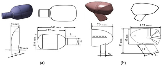
Figure 1.
Side-view mirror models used in the study: (a) Model 1, (b) Model 2.
The mirror arm dimensions of Model 1 and Model 2 are given in Table 1. While 3 levels were used for each dimension parameter, the yaw angle and the flow velocity were fixed at β = 0° and U = 30 m/s for all analyses. The Taguchi method is an experimental design and optimization method in which fractional factorial experimental plans are generally utilized. Taguchi orthogonal arrays used in experimental design contribute to efficiency by using minimum time and resources. Orthogonality is defined as matching the values of one parameter with the values of other parameters the same number of times. The experimental results obtained using the Taguchi experimental design method were evaluated by converting them to signal/noise (S/N) values. Taguchi has introduced different S/N calculations (terminologically, quality loss functions) for different targets in order to achieve the target in a way that reduces variation. An S/N value is calculated and analyzed in three different ways according to the target type of the quality variable: “smaller-the-better”, “larger-the-better”, and “nominal-the-best”. No matter which S/N type is used in the evaluation, a larger S/N value means a better experimental result. In this study, since the output variable is the drag coefficient (CD), the “smaller-the-better”-type S/N equation given in Equation (1) was employed.
where n stands for the number of experiments and yi for the values of the output variable. If a full factorial experiment plan is used to examine the 3 parameters for 3 different levels, it is necessary to conduct 33 = 27 experiments for each mirror model, and 54 experiments in total. However, L9 experiment plans generated for both models and the number of experiments were reduced to 1/3 (a total of 18) using a Taguchi L9 orthogonal array. The Taguchi L9 design effectively evaluated the effects of three parameters at three levels, but potential interactions between the parameters were not taken into account. Analyzing the interaction of parameters that could have a significant impact on aerodynamic performance is not the purpose of the current study, but it could be a valuable topic for future studies. Specific parameter levels were determined based on practical design ranges and manufacturability constraints for the side-mirrors, ensuring both aerodynamic suitability and applicability. The mean values, signal/noise (S/N) values, and variance analysis (ANOVA) were used to evaluate the effects of the parameters. In this study, the relationship between the aspect ratio, defined as the ratio of the width to the height (AR = W/H) and the drag coefficient was evaluated using the Taguchi experiment’s data by means of correlation analysis. In order to remove the effect of the third parameter (length), partial correlation was applied. In this study, Pearson’s correlation, which measures linear trends in quantitative data, and Spearman’s correlation, which measures linear and non-linear trends in ordinal data [19], were used.

Table 1.
Mirror arm dimensions of the models.
2.2. Numerical Study
In this study, side-view mirror models and solution domains were modeled using ANSYS SpaceClaim 2020R1. The body dimensions of the models were kept constant (same as the original dimensions), but the mirror arm dimensions were changed to obtain 3 levels for each. The dimensions of the solution domain were chosen considering the blockage effects. The analyses were made with side-view mirror models placed 400 mm ahead of the entrance, and 1000 × 1000 × 1250 mm solution domains. Based on the largest dimensions of each mirror arm, the blockage ratio for Model 1 and Model 2 were 2.4% and 2.2%, respectively. These values were less than the maximum 7.5% value given by Surry [20] for the blockage ratio. In addition, the computational domain was divided into 3 subdomains: inner, middle, and outer, in order to provide a graduated mesh structure. The inlet velocity and turbulent intensity of the air were determined as 30 m/s and 5%, respectively, and the outlet was considered as atmospheric environment. The top, bottom, and side walls of the flow domain and the mirror surfaces were considered no-slip smooth walls. A zero-pressure gradient was applied at the outlet of the solution area.
A graduated mesh structure with decreasing mesh density from the inner to the outer subdomain was formed in the flow domain, as shown in Figure 2. A hybrid mesh of tetrahedral and prismatic cells was generated to reduce the number of mesh elements. Prismatic cells were used at the domain boundaries and around the mirror, and the remaining volume was filled with tetrahedral cells. Approximately 90.2% of the total element number produced for each model contained tetrahedral elements and 9.8% contained prismatic elements. In order to detect the separations around the mirror model and in the wake region, the mesh density had been increased in these regions.
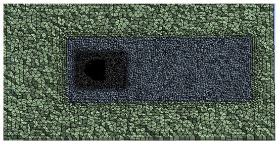
Figure 2.
Graduated mesh structure of the solution domain.
Grid Convergence Index (GCI) based on Richardson’s extrapolation was carried out for verification studies to ensure mesh independence, given by Equation (2):
where p is the order of the scheme, r is the grid refinement factor, and Fs is the factor of safety for error estimators. ε is the relative error used to compare the calculated values for two mesh structures. For both side-view mirror models, 3 different mesh element numbers were utilized as (1) fine, (2) medium, and (3) coarse. The refinement ratio was chosen as approximately 1.4 and the drag coefficient values (CD) were taken as the convergence criterion. Numbers of mesh elements and drag coefficients for Model 1 and Model 2 are given in Table 2. For both models, the ideal value of the asymptotic convergence criterion (ACC) of ACC ≈ 1 was reached. Based on the mesh sensitivity analyses and GCI values, fine grid was used in the analyses for both models.

Table 2.
Verification process: numbers of mesh elements and CD for Models 1 and 2.
A three-dimensional, steady, and incompressible turbulent flow around the side-view mirror was simulated employing a CFD-based ANSYS/FLUENT 2020R1. Conservation of mass and momentum are defined in Equations (3) and (4), respectively.
Here, ρ and P denote the density and static pressure of the fluid, respectively, while ui and uj define the fluid velocities in tensor form. is the turbulent viscosity and is defined as . The transport equations for turbulent kinetic energy (k) and dissipation rate (ε) are given in Equations (5) and (6).
In these equations, Г and Gk are defined as the turbulent kinetic energy arising from diffusion and the velocity gradient, respectively. The model constants are C1ε = 1.44, C2ε = 1.92, Cµ = 0.09, and R = 0, and the turbulent Prandtl numbers are σk = 1.0 and σε = 1.3, as recommended by Shih et al. [21]. The side-mirror aerodynamics includes complex flow structures such as flow separations, vortices, and transition flows. Because it provides more efficient solutions for both separated and free shear flows, the realizable k-ε turbulence model is used with the scalable wall function in this study. While the LES method provides very high accuracy, its efficiency is lower than that of the realizable k-ε turbulence model due to its high computational cost and time. Furthermore, unlike k-ω, SST offers higher numerical stability with lower grid requirements. It was seen that the k-ε model was the most optimal turbulence model in terms of CPU costs and time. Therefore, this model provides reliable predictions of the flows around the side-mirrors at a reasonable computational cost. In the analyses, second-order equations for turbulent kinetic energy and turbulent dissipation rate were selected and the SIMPLE solution algorithm was used.
The drag coefficient is calculated by Equation (7). In this equation, ρ is the density of the fluid, U is the free flow velocity, A is the area, and FD is the drag force.
The numerical modeling approach was validated by the study of Yu and Liu [1] and Kato et al. [10], who examined a standard mirror model numerically and experimentally, respectively. In the validation study, the geometric model and the flow conditions in the reference studies were adopted. The realizable k-ε turbulence model was used for a flow velocity of 30 m/s. The side-view mirror geometric model and the pressure coefficient variation are presented in Figure 3a and Figure 3b, respectively. The pressure coefficient values showed agreement with the values obtained in the reference numerical and experimental studies.
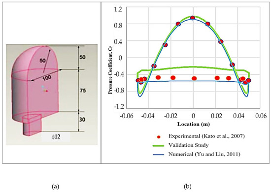
Figure 3.
Validation process: (a) Side-view mirror model, (b) pressure coefficient variation, Kato et al. [10], Yu and Liu [1].
Comparing the reference experimental results with the corresponding numerical values in the validation study, the validation metric was calculated as 0.74 for the whole mirror, and 0.82 for the front side where the flow strikes.
2.3. Experimental Study
The experiments were conducted using a 22 kW open-circuit wind tunnel designed for low-speed airflow. The airflow began in a diffuser with a 2:3 expansion ratio, then traversed through a straightening duct with screens, followed by a nozzle with a 2:1 contraction ratio and turbulence generators, and finally passed a 0.5 m long straightening duct. The tests were carried out within the test section, which initially measured 1 × 1 m2 in cross-section and 3 m in length. Plexiglass side walls were employed to ensure complete visibility of the flow area. The inlet of the test section achieved a maximum flow velocity of 35 m/s, with a turbulence intensity of 5%.
Two different side-view mirrors with the same size and shape as those used in the numerical analysis were used in the experiments. The side-view mirrors were placed at a distance of 0.4 m from the inlet. Figure 4 shows the schematic views of Model 1 and Model 2 side-view mirrors with pressure tapings of 0.5 mm diameter. The static pressure measurements on both mirror bodies were carried out using pressure taps drilled at 10 mm equal intervals on the H1 and H3 lines. In addition, those measurements were performed at 5 mm equal intervals on both mirror arms on the H2 and H3 lines. Short copper restrictors connected the pressure taps to pressure tubes with a diameter of 0.0015 m and a length of 0.5 m. The static pressures measured by a 16-channel pressure scanner system at a sampling frequency of 1000 Hz, with an uncertainty level of 0.05%. The scan duration was 360 s, resulting in an effective full-scale sampling period of approximately 1 h. A constant temperature hot-wire anemometer (CTA) and a single hot-wire probe were used for velocity measurements. The flow velocity U = 30 m/s and the yaw angle β = 0° were kept constant in all experiments.

Figure 4.
The schematic views of the side-view mirror with pressure taps: (a) Model 1, (b) Model 2.
The local pressure coefficient is calculated as follows:
where ρ is the air density, P is the static pressure measured at pressure tapings, U is the free stream velocity, and P0 is the static pressure of the free stream.
The overall uncertainty of the velocity and pressure measurements were estimated as ±2.3% and ±1.2%, respectively. The total uncertainty of the pressure and drag coefficients were also calculated as ±1.4% and ±1.5%, respectively, using the Kline and McClintock [22] uncertainty estimation method.
3. Results and Discussion
The Taguchi L9 experiment plan and the mean drag coefficient of whole mirror (body + arm) values for Model 1 and Model 2 are given in Table 3. For Model 1, the highest and lowest drag coefficient was obtained in T6 and T2 geometry, respectively. The results showed that as width and length increased, CD decreased and S/N value increased, while as height increased, CD increased and S/N value decreased. In addition, according to the slopes of the variations, it was determined that height was more effective on CD than other parameters. For Model 2, the highest and lowest CD were obtained in T1 and T9 geometry, respectively. The CD value decreased with increasing mirror arm width, but the S/N value increased. The increment in the mirror arm length and height increased the CD and decreased the S/N value. The most effective parameter on CD variation was found to be length, unlike for Model 1.

Table 3.
Experiment plan, CD and S/N values for Model 1 and Model 2.
The drag coefficients obtained from the analysis and the parameters were evaluated by variance analysis. In Table 4, the mathematical model reliability and the % contribution values of the parameters are presented for Model 1 and Model 2. According to the p values of Model 1, only the height was found to be significant (p < 0.05) in the CD variation, while all three parameters were significant in the variation in the drag coefficient flow over Model 2. In addition, the values of the determination coefficient for Model 1 (R2 ≈ 0.86) and Model 2 (R2 ≈ 0.90) showed that the mathematical model could largely explain the effects of the parameters on CD. The height was the most effective parameter among the examined parameters with 66.93% for Model 1, while the arm length was the most effective parameter for Model 2, and the contribution of length to the total change was 51.53%.

Table 4.
ANOVA table for CD (Model 1 and Model 2).
Figure 5 shows (a) velocity streamlines, (b) turbulent kinetic energies, and (c) turbulent intensities on zero total pressure iso-surfaces for the T6 and T9 geometries of Model 1. In order to determine the height effect, the flow characteristics of the geometries with the maximum (T6) and the minimum (T9) heights were compared, keeping arm length constant. The flow separation occurred around the outlet of the ellipse, where the velocity was maximum in T6 geometry, and a vortex pair formed behind the mirror arm. In the flow over T9 geometry, the flow remained on the surface for a long distance. The flow separation occurred close to the outlet of the model, and then the streamlines reattached in a short distance. In the rear side of the mirror arm, the maximum turbulent kinetic energy for T6 and T9 geometries was determined as 49.41 m2/s2 and 21.52 m2/s2, respectively. The presence of vortices in T6 geometry resulted in higher drag coefficients. The zero total pressure area of the T6 geometry was larger, especially behind the arm. In this wake region, the drag force increased while the kinetic energy decreased. It was also determined that the turbulent intensity, which causes pressure losses, increased.
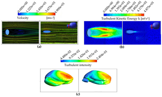
Figure 5.
T6 and T9 geometries for Model 1: (a) Velocity streamlines, (b) turbulent kinetic energies, (c) zero total pressure iso-surfaces and turbulent intensity distribution.
In Figure 6a–c, velocity streamlines, turbulent kinetic energies, and turbulent intensity distribution on zero total pressure iso-surfaces are demonstrated for T1 (maximum length) and T7 (minimum length) geometries of Model 2. The wake region of T1 geometry was longer than that of T7 geometry, and vortices were formed in this region in both geometries. The highest turbulent kinetic energy values behind the mirror arm were obtained as 89.38 m2/s2 and 51.23 m2/s2 in T1 and T7 geometries, respectively. The high turbulent kinetic energy region in the flow over T1 geometry was larger than that of T7. The mirror arm vicinity of the T1 geometry was exposed to the highest mean CD value, the zero total pressure regions expanded, and high turbulence densities were detected.
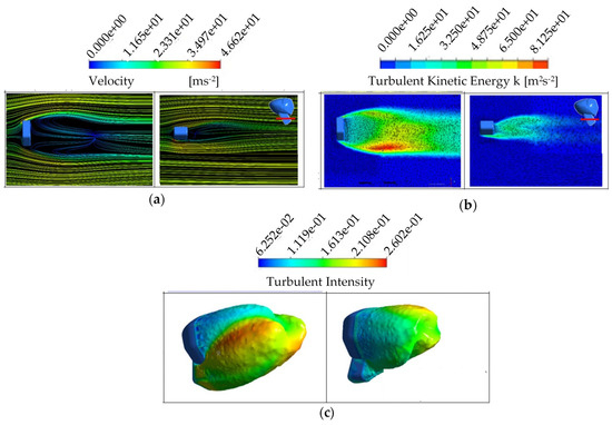
Figure 6.
T1 and T7 geometries for Model 2: (a) Velocity streamlines, (b) turbulent kinetic energies, (c) zero total pressure iso-surfaces and turbulent intensity distribution.
For Model 1 and Model 2, CD values increased with arm height, and decreased with an increase in arm width. CD values decreased as arm length increases for Model 1, unlike Model 2. This difference can be explained by the curvature of arm length for Model 1. For both models, the parameter with the lowest effect was determined as arm width. While the effects of all three parameters were significant on the drag coefficient for Model 2, only the arm height was significant for Model 1.
The variations in drag coefficient with respect to aspect ratio in the flow over Model 1 and Model 2 are given in Figure 7a and Figure 7b, respectively. Partial correlation was applied by subtracting the effect of length to determine only the effect of aspect ratio. For Model 1, Spearman correlation was employed because the data points in the scatter plot were non-linear. The correlation coefficient value of −0.850 indicated that there was a strong and negative correlation between the aspect ratio and the drag coefficient. It has been observed that the drag coefficient decreased as the aspect ratio increased, in agreement with the study of Meyer and Erland [23]. In addition, a quadratic regression curve fitting to represent the scatter plot was also performed. For Model 2 the Pearson correlation was used because of the linear data points in the scatter plot. The value of the correlation coefficient was obtained as −0.916. The drag coefficient decreased as the aspect ratio increased, similar to Model 1. A linear regression curve fitting to represent the scatter plot was also carried out.
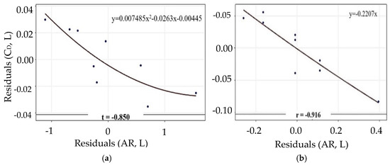
Figure 7.
Variation in drag coefficient with aspect ratio for (a) Model 1 and (b) Model 2.
The velocity streamlines the flow over T6 and T9 geometries of Model 1 are detailed in Figure 8a. The aspect ratios of the mirror with T6 and T9 geometries had a minimum and a maximum value of 0.66 and 3.33, respectively. The results showed that the high aspect ratio caused a streamlined geometry around the mirror arm and delayed the flow separations. The velocity streamlines for T4 and T9 geometries of Model 2 with same arm length are presented in Figure 8b. The T4 geometry had a minimum aspect ratio (0.23), while the T9 geometry had a maximum aspect ratio (0.79). Flow separation around the mirror arm with the higher aspect ratio of the T9 geometry occurred further compared to the T4 geometry.

Figure 8.
(a) Velocity streamlines for T6 and T9 of Model 1, and (b) for T4 and T9 of Model 2.
The numerical pressure coefficient distributions of T6 and T9 geometries of Model 1 are shown in Figure 9a–c for the H1 line, H2 line, and H3 line, respectively. Since there is no change in the mirror body, the CP values of the body on the H1 line were same in both geometries. The highest and lowest value of CP was found to be 1.03 and −0.722, respectively. The maximum and minimum values of the mirror arm on the H2 line were obtained as 0.919 and −1.95 for T6, and 0.805 and −0.857 for T9, while those of the body and arm on the H3 line were 1.07 and −0.57 for T6, and 1.04 and −0.72 for T9. The minimum values were obtained in a small region close to the upper and lower limits of the body and arm geometry on the H1 and H2 lines, respectively. The CP value of the wake side of the mirror body of both geometries was approximately −0.36 on the H1 line. The values on the wake side of the mirror arm of T6 geometry were found to be around −0.45 and −0.40 for the H2 and H3 lines, respectively, while those of T9 values were −0.10 for the H3 line, and there was no stable course for the H2 line. For all geometries, the maximum CP values occurred in the front of the mirror where the flow first struck, while the minimum values were obtained close to the boundaries of the geometry because of maximum velocity and flow separation.
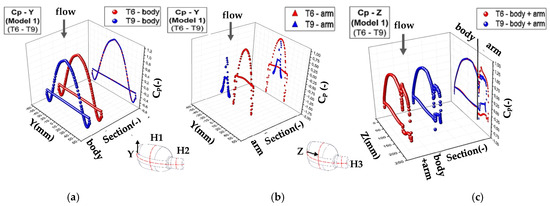
Figure 9.
The numerical pressure coefficient distributions of T6 and T9 geometries of Model 1: (a) H1 line, (b) H2 line, and (c) H3 line.
Figure 10a–c present the experimental CP distributions of the T6 and T9 geometries of Model 1 for the H1, H2, and H3 lines, respectively. The maximum values of CP on the H1 line were obtained at y = 0 as nearly 0.97, while those of minimum value were around −0.66 for both geometries. A symmetric distribution was observed on the H1 line around y = 0 for the static pressure, as stated Wang et al. [24]. The CP values of the mirror arm on the H2 line were obtained in the range of −1.91–0.90 for T6, and −0.83–0.79 for T9, respectively. The CP values of the body and arm on the H3 line were found between −0.52 and 1.02 for T6, and −0.36 and 0.99 for T9. For all geometries, the pressure coefficients took minimum values where the boundary layer separated. The mean drag coefficients of the T6 and T9 geometries based on pressure values were calculated as 0.434 and 0.381, respectively.
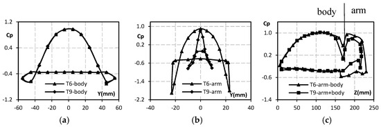
Figure 10.
The experimental pressure coefficient distributions of T6 and T9 geometries of Model 1: (a) H1 line, (b) H2 line, and (c) H3 line.
Figure 11a–c present the numerical pressure coefficient distributions of the T1 and T7 geometries of Model 2 for the H1 line, H2 line, and H3 line, respectively. The maximum CP values for the H1 line were determined as approximately 1.02 for both the T1 and T7 geometries. The minimum values were obtained close to the upper and lower limits of the mirror body and were about −1.0. The CP values of the wake side of the mirror body were −0.30 and −0.20 for the T1 and T2 geometries, respectively. The maximum CP values of the mirror arm on the H2 line for T1 geometry were equal to those of the T7 geometry value, while the minimum value of the T7 geometry was lower. The CP values on the wake side of the mirror arm of both geometries were around −0.30 for the H2 line and in the range of −0.2 to −0.3 for the H3 line. For Model 2 on the H3 line, the pressure coefficient profiles around the body and arm of the T1 and T7 geometries almost coincided. The maximum and minimum values were found to be 1.00 and −0.85, respectively, in both models.
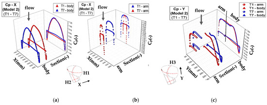
Figure 11.
The numerical pressure coefficient distributions of T1 and T7 geometries of Model 2: (a) H1 line, (b) H2 line, and (c) H3 line.
The experimental pressure coefficient distributions of the T1 and T7 geometries of Model 2 are presented in Figure 12a–c for the H1, H2, and H3 lines, respectively. The maximum CP values on the T1 geometry were determined as approximately 0.965, 0.981, and 0.995, while those on the T7 geometry were 0.995, 0.921, and 0.947 for the H1, H2 and H3 line, respectively. The lowest values were observed close to the mirror body limits to be about −1.01, −2.51, and −0.89 for the T1 geometry, and −0.94, −3.05, and −0.76 for the T7 geometry, respectively. The average drag coefficients for the T1 and T7 geometries were determined to be 0.408 and 0.251, respectively. The experimental CP curve of side-view mirrors on all lines of Model 1 and Model 2 showed similar trends with the numerical curves for both geometries. The experimental CP curves of Model 1 and Model 2 on all lines exhibited nearly identical behavior with the numerical curves for all geometries. The experimental CP values showed good agreement with the numerical values with a difference of ±2.01% for Model 1 and ±2.88% for Model 2. Moreover, the experimental mean CD values of Model 1 and Model 2 were about ±2.22% and ±2.91% lower than the numerical values, respectively.
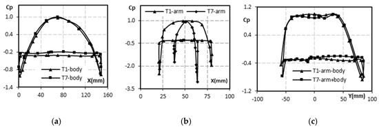
Figure 12.
The experimental pressure coefficient distributions of T1 and T7 geometries of Model 1: (a) H1 line, (b) H2 line, and (c) H3 line.
4. Conclusions
In this study, numerical and experimental aerodynamic analyses were carried out for two side-view mirror models with different geometries and mounting styles. Experiment plans were generated using fractional factorial Taguchi orthogonal arrays and the effects of the width, length, and height of the mirror arms on the drag coefficient of the side-view mirrors were investigated. In addition, the correlation analyses were performed between the drag coefficient and the aspect ratio. The flow visualization (streamlines, turbulent kinetic energy, zero total pressure regions, and turbulent intensity distribution) was performed, and pressure coefficient profiles were obtained. The results of this study can be used as a guide for aerodynamic optimization of the design of side-view mirrors in practical engineering applications. Thus, the results of this study helps automotive designers increase fuel efficiency, reduce vibration, and improve overall performance. The results obtained from the research can be summarized as follows:
- The mean drag coefficients of Model 1 and Model 2 were calculated to be between 0.359 and 0.444 and between 0.255 and 0.425, respectively, depending on the mirror arm dimensions.
- In both mirror models, mean CD values increased with arm height, while an increase in arm width reduced CD to a limited extent.
- The most effective parameters for Model 1 and Model 2 were arm height and arm length, respectively, while arm width was determined as the least effective parameter in both models.
- Arm height was the only parameter that was statistically significant on mean CD values in both mirror models. The arm width alone has little effect on mean CD values, while the aspect ratio was found to have a strong negative correlation with these values.
- High aspect ratios provided streamlined geometries around the mirror arm and delayed the flow separations.
- The variations in mirror arm dimensions caused significant changes in velocity streamlines, turbulent kinetic energy, zero total pressure regions, turbulent intensity distribution, and pressure coefficient profiles around the mirror geometries.
- In this study, the velocity was kept constant at 30 m/s. At these high velocity values, increasing the velocity is not expected to have a significant effect on CD values. However, the lower aspect ratio values result in slightly higher CD values.
- The numerical analysis results showed good agreement with the experimental values for all models and geometries.
- Future research could examine the effects of the yaw angle and higher velocities on side-view mirror aerodynamics. Conducting a factor analysis of the three-parameter interactions and examining the acoustic effects generated by different bracket geometries could also be beneficial.
Author Contributions
Conceptualization, O.Y. and M.V.E.; methodology, O.Y. and M.V.E.; software, O.Y. and M.V.E.; formal analysis, O.Y. and M.V.E.; investigation, O.Y. and M.V.E.; resources, O.Y. and M.V.E.; writing—original draft preparation, O.Y. and M.V.E.; writing—review and editing, O.Y. and M.V.E.; visualization, O.Y. and M.V.E.; project administration, O.Y. and M.V.E. All authors have read and agreed to the published version of the manuscript.
Funding
This research received no external funding.
Institutional Review Board Statement
Not applicable.
Informed Consent Statement
Not applicable.
Data Availability Statement
Data are contained within the article.
Conflicts of Interest
The authors declare no conflicts of interest.
References
- Yu, G.; Liu, D. Numerical analysis on the relationship between aerodynamic drag coefficient and 3d molding of rear view mirror. In CCIE 2011—Proceedings: 2011 IEEE 2nd International Conference on Computing, Control and Industrial Engineering; IEEE: New York, NY, USA, 2011; Volume 1, pp. 117–121. [Google Scholar]
- Khalighi, B.; Chen, K.H.; Johnson, J.P.; Snegirev, A.; Shinder, J.; Lupuleac, S. Computational and experimental investigation of the unsteady flow structures around automotive outside rear-view mirrors. Int. J. Automot. Technol. 2013, 14, 143–150. [Google Scholar] [CrossRef]
- Afgan, I.; Moulinec, C.; Laurence, D. Numerical simulation of generic side mirror of a car using large eddy simulation with polyhedral meshes. Int. J. Numer. Methods Fluids 2008, 56, 1107–1113. [Google Scholar] [CrossRef]
- Alam, F.; Jaitlee, R.; Watkins, S. Aerodynamic effects on an automotive rear side view mirror. In Proceedings of the 16th Australasian Fluid Mechanics Conference, Gold Coast, QLD, Australia, 3–7 December 2007; pp. 762–765. [Google Scholar]
- Jaitlee, R.; Alam, F.; Watkins, S. Pressure measurements on an automobile side rear view mirror. In Proceedings of the 15th Australasian Fluid Mechanics, Sydney, NSW, Australia, 13–17 December 2004; pp. 1–4. [Google Scholar]
- Su, M.; Yu, J.-D. A parallel large eddy simulation with unstructured meshes applied to turbulent flow around car side mirror. Comput. Fluids 2012, 55, 24–28. [Google Scholar] [CrossRef]
- Murukesavan, P.; Mu’Tasim, M.A.N.; Sahat, I.M. Computational analysis of an effect of aerodynamic pressure on the side view mirror geometry. IOP Conf. Ser. Mater. Sci. Eng. 2013, 50, 012039. [Google Scholar] [CrossRef]
- Ask, J.; Davidson, L. A numerical investigation of the flow past a generic side mirror and its impact on sound generation. J. Fluids Eng. Trans. ASME 2009, 131, 061102. [Google Scholar] [CrossRef]
- Kim, J.H.; Han, Y.O.; Lim, B.D. Experimental study of statistical and spectral characteristics of wake flow around the rear view side mirror of a passenger car. In Proceedings of the 5th European and African Conference on Wind Engineering, EACWE 5, Florence, Italy, 19–23 July 2009; pp. 491–494. [Google Scholar]
- Kato, C.; Murata, O.; Kokubo, A.; Ichinose, K.; Kijima, T.; Horinouchi, N.; Iida, A. Measurements of aeroacoustic noise and pressure fluctuation generated by a door-mirror model placed on a flat plate. J. Environ. Eng. 2007, 2, 278–292. [Google Scholar] [CrossRef]
- Thor, S.W.; Chippa, S.; Majage, A. Dynamic Analysis of Outside Rear View Mirror; SAE Technical Papers, 2015-26-0220; SAE International: Warrendale, PA, USA, 2015. [Google Scholar]
- Li, Q.; Yang, Z. Transient flow over generic rear view mirror using computational fluid dynamics. In Proceedings of the IEEE International Conference on Computer Science and Automation Engineering, Shanghai, China, 10–12 June 2011; pp. 742–746. [Google Scholar]
- Lin, X.; Wang, Y.; Chen, Z.; Dong, G.; Gu, Z. The flow and aerodynamic noise calculation of a generic side mirror. In Proceedings of the 11th International Conference on Computer-Aided Industrial Design and Conceptual Design, Yiwu, China, 17–19 November 2010; pp. 1278–1283. [Google Scholar]
- Yemenici, O. An experimental investigation of the flow over an automobile side rear view mirror. Int. J. Mech. Prod. Eng. 2022, 5, 52–54. [Google Scholar]
- San, Y.L.; Li, Y.M.; Xiao, S.H.; Zhang, C.Y.; Liu, Y.B. Parameter optimization and analysis of plastic separator based on EDEM-Fluent. Int. J. Simul. Model. 2024, 23, 622–633. [Google Scholar] [CrossRef]
- Witcher, K.; McAndrew, I.; Vishnevskaya, E. Aerodynamic analysis of low speed wing design using Taguchi L9 orthogonal array. MATEC Web Conf. 2018, 151, 04005. [Google Scholar] [CrossRef][Green Version]
- Wang, Z.; Wang, Y.; Zhuang, M. Improvement of the aerodynamic performance of vertical axis wind turbines with leading-edge serrations and helical blades using CFD and Taguchi method. Energy Convers. Manag. 2018, 177, 107–121. [Google Scholar] [CrossRef]
- Turan, M.K.; Erzan Topcu, E.; Karpat, F. Modelling and investigation of a driver seat suspension with negative stiffness structure. Int. J. Simul. Model. 2024, 23, 275–286. [Google Scholar] [CrossRef]
- Altman, N.; Krzywinski, M. Association, correlation and causation. Nat. Methods 2015, 12, 899–900. [Google Scholar] [CrossRef] [PubMed]
- Surry, D. Consequences of distortions in the flow including mismatching scales and intensities of turbulence. In Wind Tunnel Modelling for Civil Engineering Applications; Cambridge University Press: New York, NY, USA, 1982; pp. 137–185. [Google Scholar]
- Shih, T.-H.; Liou, W.W.; Shabbir, A.; Yang, Z.; Zhu, J. A new k–ε eddy viscosity model for high Reynolds number turbulent flows. Comput. Fluids 1995, 24, 227–238. [Google Scholar] [CrossRef]
- Kline, S.J.; McClintock, F.A. Describing uncertainties in single sample experiments. Mech. Eng. 1953, 75, 3–8. [Google Scholar]
- Meyer, R.W.; Erland, S. Induced drag in two dimensions in ideal fluids. J. Phys. Commun. 2019, 3, 115005. [Google Scholar] [CrossRef]
- Wang, Y.; Gu, Z.; Li, W. Evaluation of aerodynamic noise generation by a generic side mirror. World Acad. Sci. Eng. Technol. 2010, 61, 364–371. [Google Scholar]
Disclaimer/Publisher’s Note: The statements, opinions and data contained in all publications are solely those of the individual author(s) and contributor(s) and not of MDPI and/or the editor(s). MDPI and/or the editor(s) disclaim responsibility for any injury to people or property resulting from any ideas, methods, instructions or products referred to in the content. |
© 2025 by the authors. Licensee MDPI, Basel, Switzerland. This article is an open access article distributed under the terms and conditions of the Creative Commons Attribution (CC BY) license (https://creativecommons.org/licenses/by/4.0/).