A Novel Desired-State-Based Car-Following Model for Describing Asymmetric Acceleration and Deceleration Phenomena

Abstract

This paper addresses the modeling challenge of significant asymmetry between acceleration and deceleration processes in car-following behavior by proposing an Asymmetric Acceleration and Deceleration Car Following (AAD-CF) model. The model characterizes driving decisions using both desired speed and desired spacing, and incorporates an asymmetric correction factor to capture differences in acceleration and deceleration behavior. Based on real vehicle trajectory data from the I-80 dataset, the model was compared at the microscopic level against classical models such as Gipps in terms of trajectory fitting error. The results show that the AAD-CF model consistently achieves lower trajectory fitting errors across different simulation time-steps, with error reduction exceeding 10%. At the macroscopic traffic flow level, the model successfully reproduced three-phase traffic flow states—free flow, synchronized flow, and wide moving jams. By implementing both startup and emergency braking scenarios, it was further revealed that braking waves propagate approximately 40% faster than startup waves, demonstrating asymmetric wave propagation. This study provides quantitative evidence for understanding the intrinsic relationship between microscopic driving behavior and macroscopic traffic phenomena, and the proposed model can support traffic simulation systems and theoretical analysis.

1. Introduction

A deep understanding of microscopic car-following dynamics is vital for modeling and predicting complex traffic flow. As a fundamental tool for describing longitudinal vehicle interactions, car-following models are widely used in traffic planning, autonomous driving, and safety assessment [1,2].

A number of car-following models have been developed, such as the Gipps model [3], the optimal velocity model (OVM) [4], and intelligent driver model (IDM) [5] have formed the theoretical basis for car-following behavior. Building on these, many improved models introduce features like reaction delay [6], multi-leader effects [7], and velocity–spacing coupling [8,9] to enhance behavioral realism.

However, most classical car-following models are built on the implicit assumption that drivers’ responses to the stimuli of a leading vehicle are symmetric in acceleration and deceleration phases [10]. This implies that drivers react with equal intensity to sudden deceleration and acceleration of the leading vehicle. However, empirical studies consistently reveal an inherent asymmetry in risk perception, drivers are generally risk-averse and respond more sensitively and aggressively to deceleration stimuli, as these are directly related to safety. In contrast, responses to acceleration stimuli are typically more conservative and delayed, since missing an acceleration opportunity is far less critical than risking a rear-end collision [11]. This cognitive and behavioral asymmetry represents a fundamental feature that symmetric models fail to capture.

In the process of building a car-following model that considers the asymmetric characteristics of acceleration and deceleration, there are two key issues to be resolved. The first is discrimination between acceleration and deceleration states. This refers to the driver’s asymmetric response to acceleration and deceleration. The model requires a clear mechanism to determine whether the driver is in an acceleration decision mode or a deceleration decision mode. The second is the construction of an asymmetric response function, which involves how to reflect the driver’s differentiated reactions during acceleration and deceleration phases in the dynamic equations.

To address these challenges, this study introduces two hypotheses. H1: Asymmetry can be captured by distinguishing between acceleration and deceleration parameters. H2: Compared with symmetric models, incorporating acceleration–deceleration asymmetry can significantly reduce the fitting error of car-following trajectories.

Based on this analysis, we propose the Asymmetric Acceleration–Deceleration Car-Following Model (AAD-CF). The contributions of this model are twofold. First, it considers the coupling between speed and spacing when defining the desired state, making the desired state more consistent with drivers’ actual perception. Second, it introduces asymmetric correction factors in both the speed and spacing dimensions to adjust drivers’ response intensity under different states, thereby dynamically modeling asymmetric reactions in acceleration and deceleration.

The remainder of this paper is organized as follows: Section 2 reviews related work on car-following models. Section 3 introduces the AAD-CF model. Section 4 presents microscopic trajectory simulations and compares fitting errors with IDM, OVM, and Gipps. Section 5 extends the analysis to macroscopic traffic flow simulations. Section 6 concludes the study.

2. Related Work

2.1. Comparison with Mainstream Car-Following Models

From a modeling perspective, car-following models can generally be classified as rule-based models and data-driven models. Rule-based models rely on assumptions that reflect the characteristics of car-following behavior and describe driver behavior through explicit mathematical formulations. These models offer interpretability and theoretical insight into the mechanisms of car-following. In contrast, data-driven models extract general behavioral patterns directly from empirical data. Although they often achieve higher prediction accuracy, they offer limited capability in advancing our understanding of driver behavior [12].

Among rule-based models, three categories are commonly distinguished based on the underlying assumptions: desired distance models, desired velocity models, and desired state models [13].

In desired distance models, the Gipps model is a representative example [3,14]. It assumes that the spacing between the following vehicle and the leading vehicle must remain above a minimum safe distance, and the acceleration is calculated accordingly to avoid collisions, even under abrupt deceleration of the lead vehicle. Recent studies have focused on improving the safety and flexibility of the Gipps model. For instance, Shah et al. [3] proposed a collision-adjusted Gipps model to mitigate the risk of crashes in dense traffic. Samson [15] employed a Bayesian framework to estimate model parameters, enhancing the model’s predictive power and uncertainty quantification. However, their parameter rigidity limits their ability to reproduce complex traffic states, particularly synchronized flow, and they fail to capture asymmetric acceleration–deceleration behavior.

In the category of desired velocity models, classical examples include the Newell model [16], the optimal velocity model (OVM), the generalized force model (GFM) [17], and full velocity difference model (FVD) [18]. In OVM, the acceleration of a vehicle is determined by the difference between its current velocity and a desired optimal velocity, making the model structurally indirect but well-suited for theoretical analysis and nonlinear stability studies. Recent improvements include incorporating reaction delay and nonlinear sensitivity mechanisms. Abdelhalim et al. [4] introduced a time to collision-based safety mechanism and proposed a safe optimal velocity model, which enhanced the model’s applicability to real-world traffic scenarios. The desired speed models are simple and analytically tractable but often generate unrealistic oscillations in dense traffic, leading to numerical instability.

The intelligent driver model (IDM) is a typical example of a desired state model, as it jointly considers the desired velocity and space. Recent extensions to IDM have focused on parameter calibration and dynamical enhancements. For example, Zhang et al. [5] proposed the MA-IDM, which combines Bayesian inference and high-resolution trajectory data to improve the model’s ability to fit real driving behavior. Jiahao et al. [19] extended IDM from longitudinal to both longitudinal and lateral dimensions, enabling it to model complex driving scenarios.IDM remains one of the most influential models, with intuitive parameters and good stability, but its assumption of symmetric driver response reduces its realism and constrains its ability to reproduce three-phase traffic phenomena.

In summary, mainstream models have greatly advanced car-following theory, but share several limitations: (1) most assume symmetric acceleration–deceleration responses, ignoring empirically observed asymmetry; (2) they have limited ability to simultaneously capture microscopic behavioral heterogeneity and macroscopic traffic patterns; and (3) some models exhibit instability under high-density conditions. To overcome these issues, we propose an asymmetric model that explicitly distinguishes acceleration and braking responses. By incorporating asymmetric behavioral traits, the AAD-CF improves trajectory fitting accuracy and achieves higher consistency with observed traffic phenomena at the macroscopic level.

2.2. Relation to Kerner’s Three-Phase Traffic Theory

Kerner’s three-phase traffic theory (TPT) provides a novel framework for explaining complex nonlinear phenomena in traffic flow [20]. It divides traffic states into Free Flow (F), Synchronized Flow (S), and Wide Moving Jam (J), emphasizing that the F–S transition involves a multivalued region rather than being determined by a single fundamental diagram. This framework challenges the traditional “one-to-one flow–density relation” assumption, highlighting the multivaluedness of synchronized flow and the uncertainty of state transitions. Extensive empirical evidence supports TPT in describing self-organizing evolution of congestion [21].

Nevertheless, TPT faces limitations in modeling and application. It primarily emphasizes empirical generalizations and macroscopic descriptions while lacking rigorous microscopic behavioral mechanisms. Moreover, its simulation implementations often rely on cellular automata, which inadequately capture the continuity and asymmetry of driver responses in acceleration and braking.

In contrast, the AAD-CF model is grounded in drivers’ desired states and introduces asymmetric correction mechanisms for speed and spacing. At the microscopic level, it captures asymmetric acceleration–deceleration behavior. At the macroscopic level, it reproduces the transitions among F, S, and J states described by TPT. By starting from behavioral mechanisms, the AAD-CF inherits TPT’s strength in explaining macroscopic patterns while addressing its limitations in microscopic modeling. This provides a promising pathway for integrating driver behavior mechanisms with three-phase traffic simulations.

2.3. Relation to Asymmetric Acceleration–Deceleration Behavior

Several studies have explored asymmetric acceleration–deceleration behavior through empirical analysis and theoretical modeling [22]. On the empirical side, Siuhi et al. [10], based on the US-101 dataset, found that drivers tend to react more quickly and sensitively during deceleration. Huang et al. [23] analyzed the NGSIM dataset and confirmed that variables such as spacing, speed change rate, and response delay significantly differ between acceleration and deceleration phases.

3. Methods

In real traffic, drivers show clear asymmetry between acceleration and braking. This phenomenon reflects underlying differences in risk perception and decision-making psychology. To capture the trait, this study uses the desired car-following state as the decision basis and adds an asymmetric response mechanism to build a dynamically adaptive model. By adding correction factors in speed and spacing, the model adjusts sensitivity in acceleration and deceleration phases, enabling dynamic modeling of acceleration–deceleration asymmetry.

3.1. Desired Following State

The essence of acceleration deceleration asymmetry lies in the driver’s perception and response to the deviation between the desired car-following state and the actual car-following state. Driver behavior is not solely adjusted based on the instantaneous spacing or relative speed; rather, it is governed by the difference between the current state and the driver’s subjective expectations. This desired state serves as a behavioral threshold, determining whether the driver chooses to accelerate or decelerate under the given context, as well as the intensity of the response. This cognitive mechanism simultaneously accounts for both speed and spacing, and is a critical feature for accurately characterizing real-world car-following behavior. Therefore, this study introduces a speed–spacing coupling feature to reconstruct the computation of the desired car-following state.

Let $v_f(m/s)$ and $v_l(m/s)$ denote the speeds of following and leading vehicles, respectively. And $s\left(m\right)$ is the distance between two vehicles. And $s_m\left(m\right)$ denotes the minimum safe distance [14], as shown in Equation (1). Define the speed difference as $\Delta v=v_l-v_f$, and the gap deviation as $\Delta s=s-s_m$.

$$s_m={\displaystyle \frac{v_f^2}{2b_f}}+v_f*r_t+s_0+L_l-{\displaystyle \frac{v_l^2}{2b_l}}$$

(1)

where $b_f(m/s^2)$ represents the deceleration adopted by the following car, $b_l(m/s^2)$ represents the estimated maximum deceleration of the leading vehicle, $r_t\left(s\right)$ represents reaction time, $L_l$ is the length of the leading vehicle, and $s_0\left(m\right)$ is the parking distance.

Regarding the desired speed ($v_e$), previous studies have indicated that following vehicle’s desired speed typically tends to approach the speed of the leading vehicle [24]. Building upon this observation, this study introduces the coupled influence of both speed difference and spacing difference.

When both $\Delta v>0$ and $\Delta s>0$, the leading vehicle is faster or the spacing is relatively large, making it harder for following vehicle to close the gap, the desired speed should be increased. Conversely, when both values are negative, a potential collision risk is implied, and the desired speed should be reduced. Accordingly, the desired speed is defined, as shown in Equation (2). In Equation (2), parameter ${\eta }_s^1$ represents the time required by following driver to compensate for the spacing difference. Measured in seconds, it reflects the driver’s aggressiveness in closing the gap; a smaller ${\eta }_s^1$ indicates a more aggressive driving style. The parameter ${\lambda }_v^1$ denotes the weighting factor of speed difference in influencing the desired speed.

$$v_e=v_l+{\lambda }_v^1\Delta v+{\displaystyle \frac{\Delta s}{{\eta }_s^1}}$$

(2)

For the modeling of desired spacing ($s_e$ (m)), this paper draws on the minimum safe distance commonly used in the Gipps model and the IDM as a foundation. In addition, the model incorporates correction terms based on variation trends of speed difference and spacing difference. When $\Delta v>0$, the vehicle is faster and the gap is widening, and the desired spacing should be reduced accordingly. When $\Delta s>0$, meaning the current gap exceeds braking distance, it reflects the driver’s preference for a larger safety buffer, and desired spacing should be appropriately increased. The final expression for calculating desired spacing is given in Equation (3).

$$s_e=s_m+{\eta }_s^2\Delta s-{\lambda }_v^2\Delta v$$

(3)

where ${\lambda }_v^2\left(s\right)$ and ${\eta }_s^2$ are the parameters to be calibrated.

Once the desired speed and spacing are determined, driver’s behavioral adjustment can be evaluated from two dimensions: speed and spacing. The speed deviation is represented by $v_e-v_f$, and the spacing deviation is represented by $s-s_e$. Driver’s decision making is not based on a single variable but rather on the combined deviation from desired state. When actual speed is lower than desired speed, or actual spacing exceeds desired spacing, the driver tends to accelerate. Conversely, when actual speed is higher than desired speed, or spacing is smaller than desired spacing, driver tends to decelerate.

3.2. Asymmetric Correction Factors

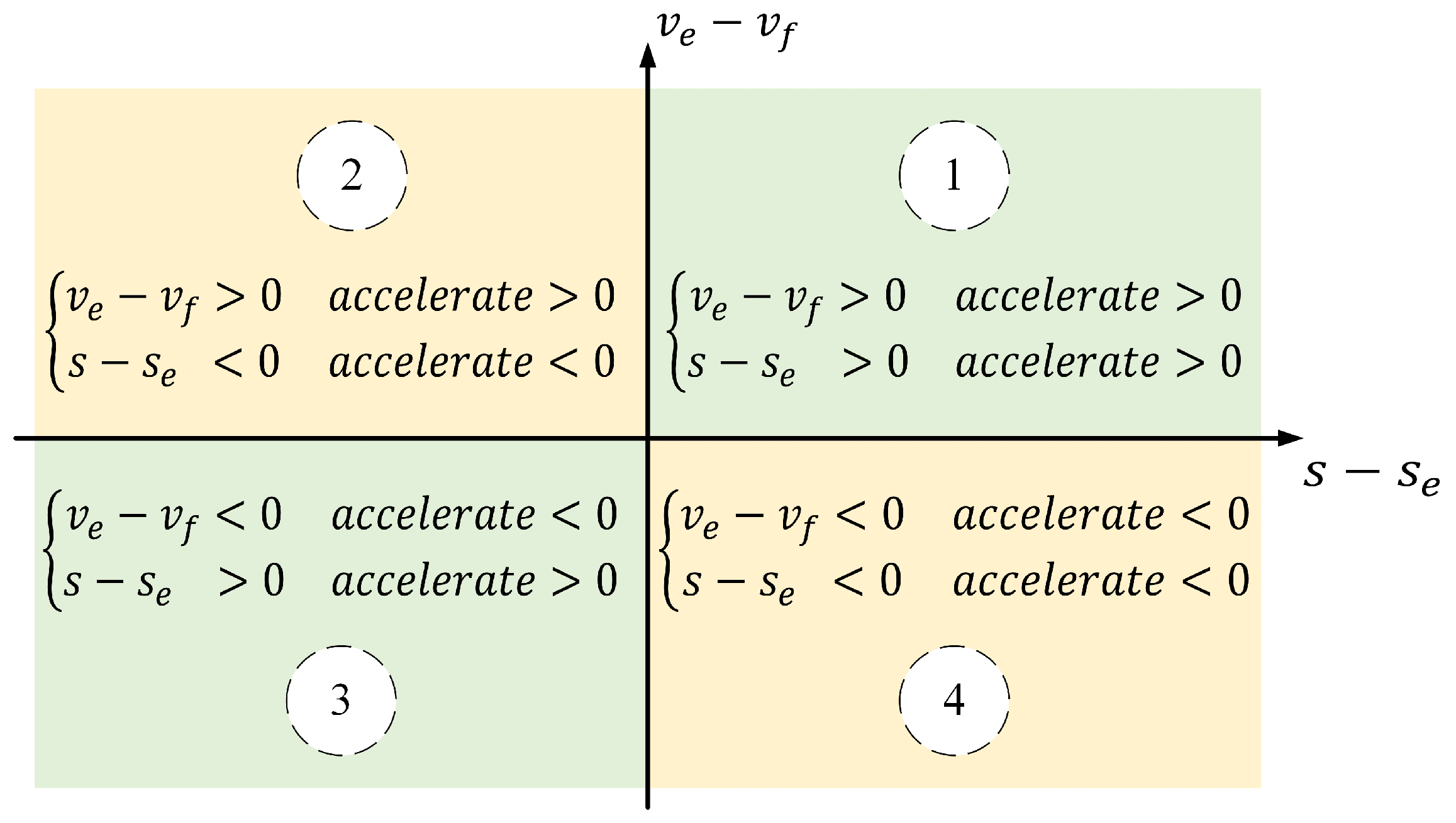
Based on the relationship between speed and spacing deviations, the car-following state is categorized into four typical scenarios, as illustrated in Figure 1. In the first and third quadrants, the deviations in speed and spacing are in the same direction, corresponding to cases of dual acceleration and dual deceleration, respectively. In these situations, the driver’s behavioral decision is relatively straightforward. However, in the second and fourth quadrants, speed and spacing deviations are in opposite directions, requiring the driver to balance between two factors in order to decide whether to accelerate or decelerate.

To more realistically capture this asymmetric response mechanism, this study introduces a dual asymmetric response adjustment mechanism, incorporating both a speed correction factor and a spacing correction factor into the model.

Specifically, this study employs asymmetric correction factors to distinguish between acceleration and deceleration behaviors. When the vehicle is in an acceleration state, the correction factor is constrained within the range $[0,1]$. When in a deceleration state, it is constrained within $[1,2]$. Thereby reflecting the driver’s typically stronger response in deceleration scenarios. To ensure smoothness and boundedness of correction factors, a sigmoid function is adopted for their formulation. The output is then scaled by a coefficient to normalize the result to the interval $[0,1]$. As a result, expressions for speed correction factor, $a_e^v$, and spacing correction factor, $a_e^s$, are defined as shown in Equation (4).

$$\left\{\begin{array}{c}{a}_e^v={\displaystyle \frac{1}{2}}\left({\displaystyle \frac{2}{1+ex{p}^{v_e-v_f}}}+{\displaystyle \frac{2}{1+ex{p}^{s_e-s}}}\right)\hfill \\ a_e^s={\displaystyle \frac{1}{2}}\left({\displaystyle \frac{2}{1+ex{p}^{v_f-v_e}}}+{\displaystyle \frac{2}{1+ex{p}^{s-s_e}}}\right)\hfill \end{array}\right.$$

(4)

3.3. AAD-CF

Based on the aforementioned mechanism, the proposed AAD-CF model is formulated as shown in Equation (5). Here, $k_v$ and $k_s$ represent the driver’s sensitivity to speed deviation and spacing deviation, respectively. The core model employs the hyperbolic tangent ($tanh$) function to represent the acceleration response, ensuring the model output is bounded within the interval $[-1,1]$. By incorporating the maximum acceleration, $a_{max}$, the actual vehicle acceleration value is obtained.

$$a={\displaystyle \frac{a_{max}}{2}}\left\{\mathit{tanh}\left[k_v{a}_e^v(v_e-v_f)\right]+\mathit{tanh}\left[k_s{a}_e^s(s-s_e)\right]\right\}$$

(5)

4. Microscopic Trajectory Simulation Results

To validate the accuracy and stability of the AAD-CF model, simulation errors of vehicle trajectories are compared with mainstream models such as Gipps, OVM, and IDM based on the NGSIM dataset [25]. In the simulation process, the time step ($\Delta \tau$ (s)) is set to 0.1, 0.5, 1, and 1.5, respectively. A smaller simulation error indicates higher model accuracy. A smaller simulation error indicates higher model accuracy, while a smaller standard deviation of the error and less variation across time steps reflect stronger model stability and universality.

4.1. Data

The data for simulation is based on I-80 dataset belonging to the NGSIM project, which has been recalculated and smoothed [26]. The car-following segments are extracted according to following criteria. Only cars are selected. The fields $FrameID$, $VehicleID$ and $LeaderID$ are used to match each follower-leader pair into a single row. Only segments with a car-following duration greater than 20 s are retained. Segments with a headway exceeding 100 m are excluded. A statistical summary of the selected car-following segments is provided in

Table 1. Statistics of car-following segments in I-80 dataset.

Number of car-following segments	Average following time (s)	Average driving distance (m)
1684	42.0148	283.7348
Average driving speed (m/s)	Average acceleration (m/s2)	Average net space (m)
6.9643	−0.0158	18.3205

.

4.2. Parameter Calibration

For each car-following segment, model parameters are calibrated using a genetic algorithm (GA). The GA settings are as follows: each generation consists of 100 chromosomes, and the algorithm iterates for 100 generations. The Root Mean Squared Error (RMSE), defined in Equation (6), is used to measure simulation error. A lower RMSE indicates a better fit and corresponds to a higher fitness of the chromosome.

The structures of Gipps, OVM, and IDMs are given in Equations (7)–(9), respectively. The parameters to be calibrated for each model, along with their corresponding value ranges, are listed in

Table 2. Parameters to be calibrated and range of value.

Gipps	Parameter	${\mathit{a}}_{\mathit{m}\mathit{a}\mathit{x}}$	${\mathit{b}}_{\mathit{f}}$	${\mathit{b}}_{\mathit{l}}$	${\mathit{s}}_0$	${\mathit{v}}_{\mathit{m}\mathit{a}\mathit{x}}$	${\mathit{r}}_{\mathit{t}}$
	Unit	m/s2	m/s2	m/s2	m	m/s	s
	Value range	[0,8]	[0,8]	[0,8]	9	[10, 40]	[0.5,3]
OVM	Parameter	$\alpha$	$V_1$	$V_2$	$C_1$	$C_2$
	Unit		m/s	m/s
	Value range	[0.5,4]	[0,30]	[0,30]	[0,4]	[0,4]
IDM	Parameter	$a_{max}$	$v_{max}$	$\delta$	$r_t$	$s_0$	$b_f$
	Unit	m/s2	m/s		s	m	m/s2
	Value range	[0,8]	[10,40]	[0,6]	[0.5,3]	[0,10]	[0,8]
AAD-CF	Parameter	$a_{max}$	$k_v$	$k_s$	$r_t$	$s_0$	$b_f$
	Unit	m/s2			s	m	m/s2
	Value range	[0,8]	[0,1]	[0,1]	[0.5,3]	[0,3]	[0,8]
	Parameter	$b_l$	${\lambda }_v^1$	${\lambda }_v^2$	${\eta }_s^1$	${\eta }_s^2$
	Unit	m/s2		s	s
	Value range	[1,8]	[1,20]	[0,3]	[0,3]	[0,3]

. The parameter bounds are set relatively wide to ensure that optimal parameter combination can be effectively identified during the optimization process.

$$RMS{E}_s=\sqrt{{\displaystyle \frac{1}{N}}\sum _{i=1}^N\sum _{t=1}^T{(y_i^t-{\widehat{y}}_i^t)}^2}$$

(6)

where $RMS{E}_s$ is the simulation error for calculating the vehicle position, N is the total number of following vehicles, and T represents the duration of following segment. $y_i^t$ and ${\widehat{y}}_i^t$ are the actual and simulated positions of the $i-th$ vehicle at time t, respectively.

$$\left\{\begin{array}{c}{v}_a=v_f+2.5a_{max}{r}_t(1-{\displaystyle \frac{v_f}{v_{max}}})\sqrt{0.025+{\displaystyle \frac{v_f}{v_{max}}}}\hfill \\ v_b=-b_f({\displaystyle \frac{r_t}{2}}+\theta )+\sqrt{b_f^2({\displaystyle \frac{r_t}{2}}+\theta )+b_f\left[2(s-s_0-l_l)-r_t{v}_f+{\displaystyle \frac{v_l^2}{b_l}}\right]}\hfill \\ v_f=Max(0,Min\{v_a,v_b\})\hfill \end{array}\right.$$

(7)

where $a_{max}$ is the maximum acceleration, $r_t$ is the reaction time, $v_{max}$ is the maximum driving speed, $b_f$ and $b_l$ are the maximum deceleration of following and leading vehicle, $s_0$ is parking distance, and $l_l$ is length of the leading vehicle.

$$\left\{\begin{array}{c}a=\alpha \{V\left(s\right)-v_f\}\hfill \\ V\left(s\right)=V_1+V_{2}tanh\left[C_1(s-l_l)-C_2\right]\hfill \end{array}\right.$$

(8)

where $V_1$, $V_2$, $C_1$, $C_2$ are parameters to be calibrated.

$$a_f=a_{max}\left[1-{\left({\displaystyle \frac{v_f}{v_{max}}}\right)}^{\delta }-\left({\displaystyle \frac{s_0+v_f{r}_t-\frac{v_f\Delta v}{2\sqrt{a_{max}{b}_f}}}{s-l_l}}\right)\right]$$

(9)

where $\delta$ is parameter to be calibrated.

4.3. Statistics and Analysis of Simulation Errors

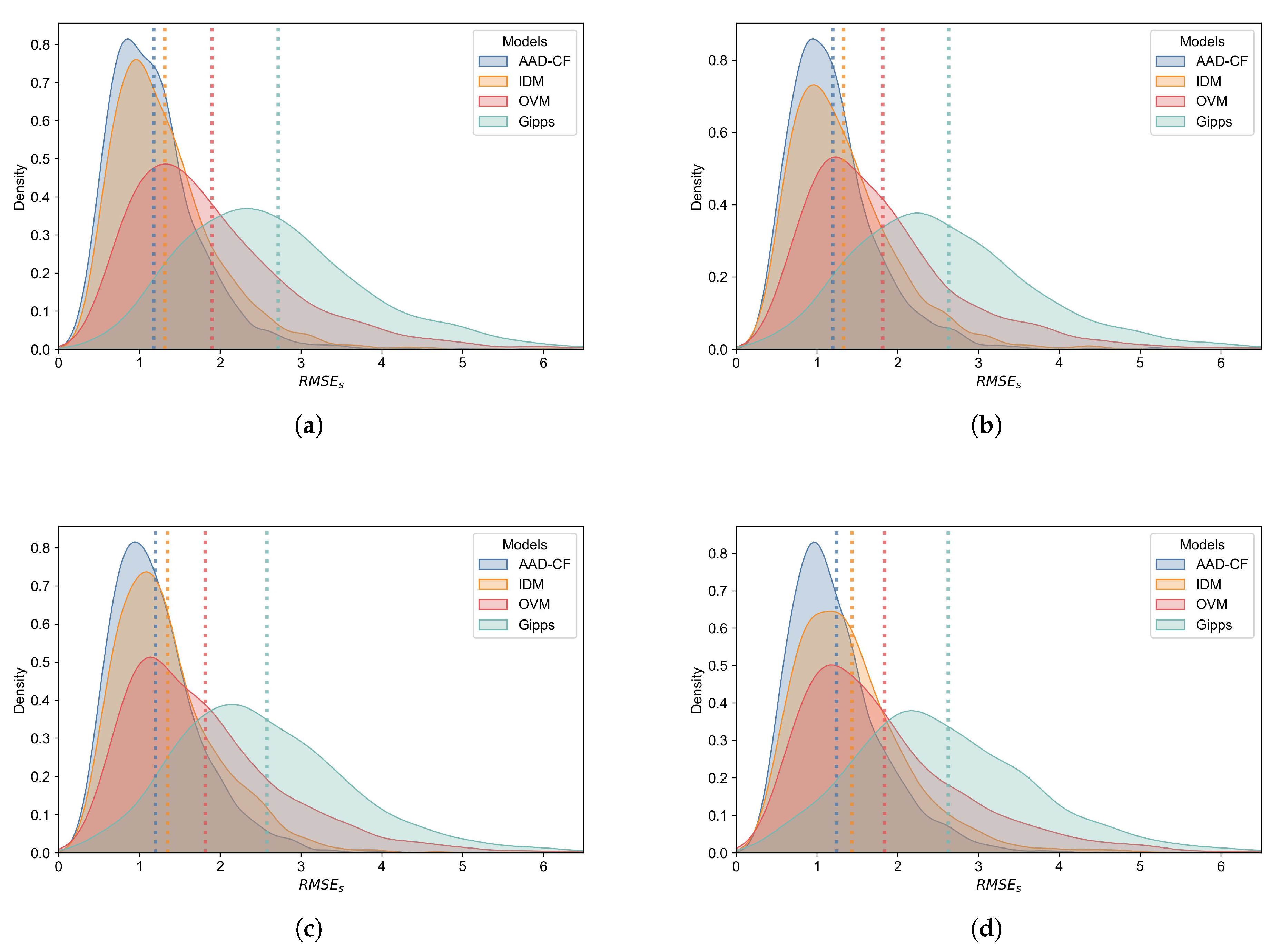
The distribution of simulation errors for each model is shown in Figure 2, where the vertical lines indicate the mean simulation error for each model.

The simulation results demonstrate that the AAD-CF model consistently exhibits the lowest simulation error across all tested time step sizes ($\Delta \tau$ = 0.1 s, 0.5, 1.0 s, 1.5 s). This indicates that the AAD-CF model achieves the highest simulation accuracy, exhibits better individual adaptability, and is more capable of capturing diverse driving behaviors.

The mean and standard deviation of the simulation errors are summarized in

Table 3. Comparison table of simulation error r$RMS{E}_s$.

$\mathbf{\Delta }\mathit{\tau }$ (s)		IDM	OVM	Gipps	AAD-CF
0.1	Mean value	1.3098	1.8984	2.7152	1.1745 (10.33%)
	Standard deviation	0.6550	1.0552	1.2714	0.5623
0.5	Mean value	1.3285	1.8151	2.6289	1.1935 (10.16%)
	Standard deviation	0.6654	1.0077	1.2239	0.5603
1.0	Mean value	1.3447	1.8144	2.5766	1.2001 (10.75%)
	Standard deviation	0.6653	1.0247	1.1852	0.5460
1.5	Mean value	1.4317	1.8353	2.6257	1.2409 (13.33%)
	Standard deviation	0.7326	1.0684	1.2089	0.5888

. A comparison of the mean simulation errors shows that, under time steps of 0.1 s, 0.5 s, 1.0 s, and 1.5 s, the AAD-CF model reduces the error by 10.33%, 10.16%, 10.75%, and 13.33%, respectively, compared to IDM. This indicates that as the simulation time step increases, the error of classical models rises significantly, while AAD-CF model maintains high stability. This also indicates that AAD-CF is not only suitable for task scenarios with fast simulation frequencies, but also maintains higher reliability in task scenarios with lower simulation frequencies.

Further comparison of the standard deviation from simulation errors reveals that the AAD-CF model consistently achieves the lowest standard deviation across all time steps. This result further demonstrates that the AAD-CF model outperforms other classical car-following models in terms of error stability and exhibits superior overall robustness.

4.4. Sensitivity Analysis of Parameters

To further investigate the influence of each parameter in the AAD-CF model on car-following behavior, a global sensitivity analysis is conducted using the Sobol variance-based method. The ranges of 11 parameters in AAD-CF model are listed in Table 2. A total of 24,000 parameter sets are generated in the parameter space using latin hypercube sampling. 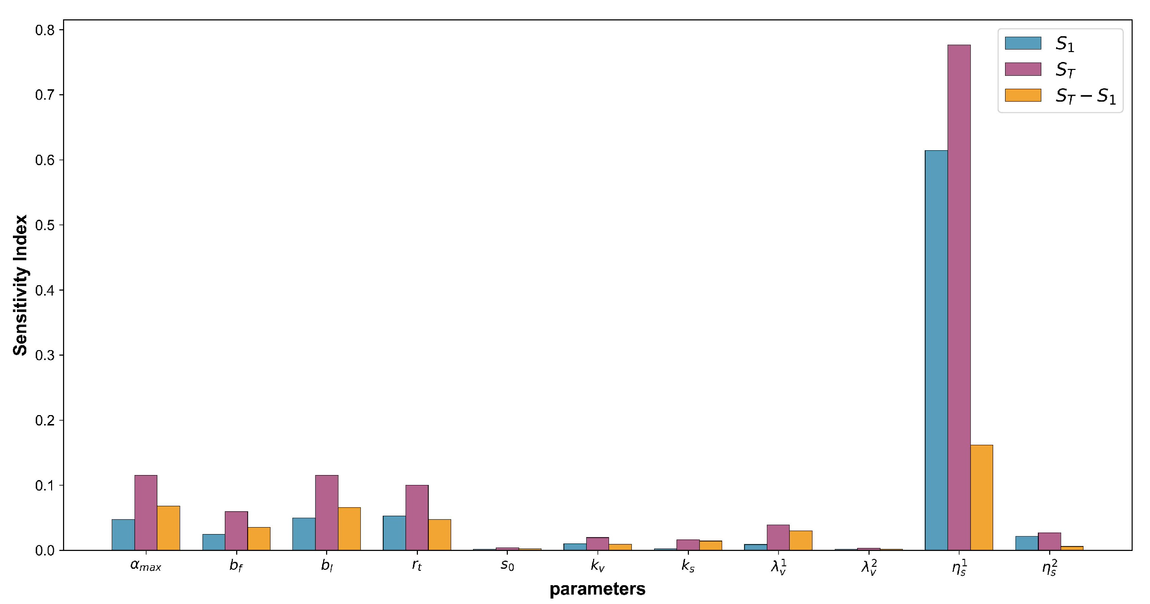For each parameter set, the trajectory fitting error ($RMS{E}_s$) is computed based on car-following segments from the I-80 dataset. The first-order and total-order Sobol indices are calculated and illustrated in Figure 3, where $S_1$ denotes the first-order index and $S_T$ denotes the total-order index.

As shown in Figure 3, the parameter ${\eta }_s^2$ exhibits a first-order Sobol index of 0.6145, which is significantly higher than that of all other parameters. This indicates that ${\eta }_s^2$ alone explains approximately 61% of the variance in AAD-CF model. Even minor fluctuations in this parameter can substantially affect the model outputs, suggesting that it should be prioritized during calibration. The variation of ${\eta }_s^2$ primarily influences the driver’s desired headway, highlighting that drivers tend to prioritize maintaining a safe distance over travel efficiency.

Additionally, parameters $a_{max}$, $b_f$, $b_l$, and $r_t$ show relatively high first-order indices, reflecting their roles in refining the dynamic characteristics of car-following behavior. Overall, parameter interactions are relatively weak, implying that the functions of model parameters are largely independent. This property is favorable for both practical calibration and interpretability in applications.

5. Macroscopic Traffic Flow Simulations

To validate the effectiveness of the proposed AAD-CF model in macroscopic traffic flow simulations, three representative scenarios are designed: (1) A vehicle platoon starting scenario, to observe the propagation of start waves. (2) An emergency braking scenario, to examine the propagation of braking waves and potential collisions. (3) A traffic evolution scenario based on the three-phase traffic theory, to test the model’s applicability under complex traffic conditions.

The parameters of AAD-CF model are set as follows: $a_{max}$ = 3 m/s², $l_l$ = 5.0 m, $b_f$ = 3 m/s², $b_l$ = 5 m/s², $r_t$ = 1 s, $s_0$ = 1 m, ${\lambda }_v^1$ = 4 s and the sensitivity parameters $k_v$, $k_s$ are set to 0.1, and parameters ${\lambda }_v^2$, ${\eta }_s^1$, ${\eta }_s^2$ are all set to 1.

5.1. Vehicle Platoon Starting Scenario

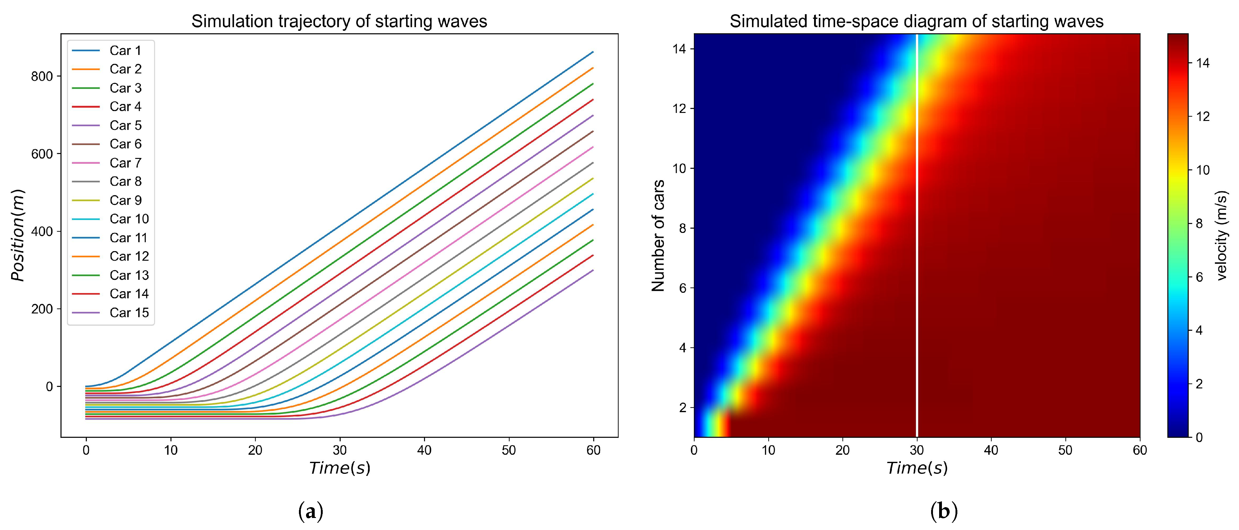
The simulation considered a platoon of 15 vehicles, each with a length of 5 m and an initial headway of 6 m. At the beginning, all vehicles were at rest, with both velocity and acceleration set to zero. After the simulation started, the leading vehicle accelerated at 3 (m/s²) until reaching 15 (m/s), after which it maintained a constant speed. The simulation step size was set to 0.1 s. The trajectories and speeds of all vehicles were recorded, and a space–time diagram was plotted (as Figure 4). The results indicate that the 15th vehicle started moving at approximately 30 s, suggesting that the start wave took around 30 s to propagate through the entire platoon.

5.2. Emergency Braking Scenario

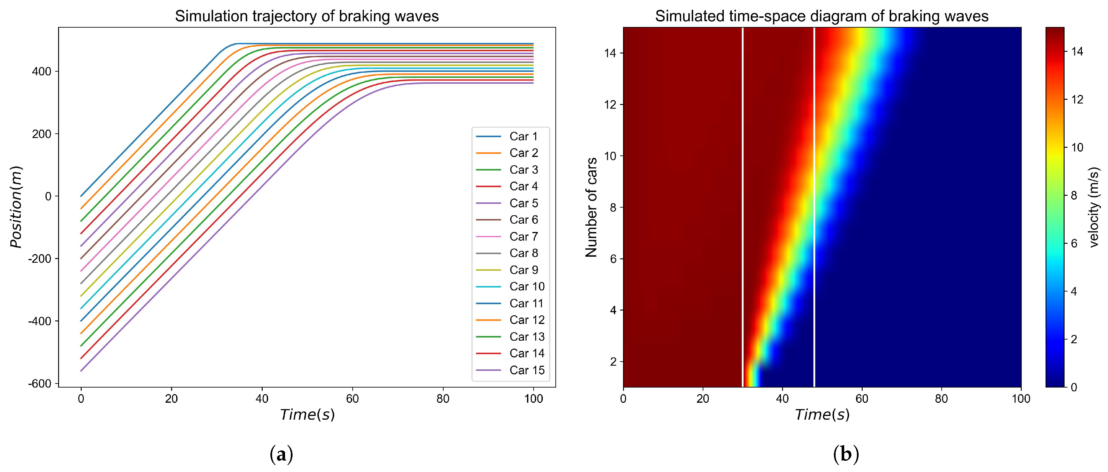
In this case, the platoon also consisted of 15 vehicles, each traveling initially at 15 (m/s) with an inter-vehicle spacing of 40 m. During the first 30 s, the leading vehicle maintained constant speed while the others followed. At t = 30 s, the leader applied an emergency brake with a deceleration of 3 (m/s²) until coming to a complete stop. The resulting vehicle trajectories and velocity profiles are shown in Figure 5. The results reveal that the braking wave propagated through the platoon in only 18 s, compared to 30 s for the start wave. This finding confirms the asymmetric nature of acceleration and deceleration behavior at the macroscopic level. Importantly, no collisions were observed in the trajectories, even under emergency braking.

5.3. Three-Phase Traffic Flow Scenario

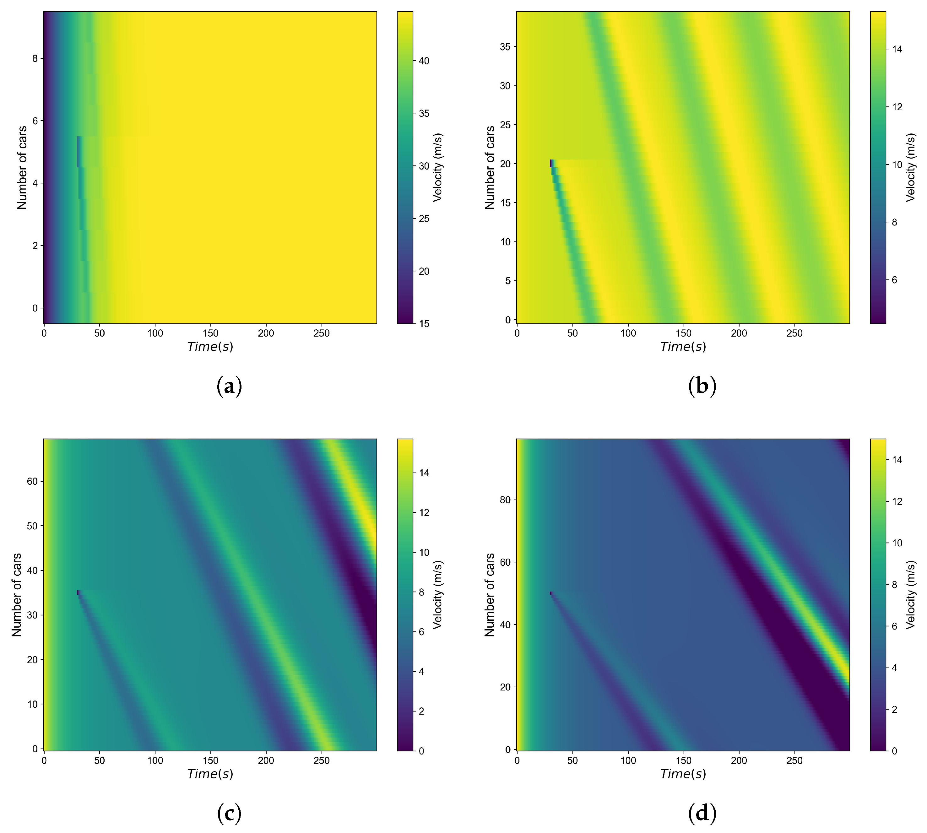
To avoid boundary effects on traffic evolution, the simulation environment was set as a single-lane ring road of length L = 1000 (m). By adjusting the number of vehicles N, different density levels were constructed to induce typical three-phase traffic states. Four cases were tested with $N=10,40,70$ and 100, representing sparse to high-density traffic. The simulation step size was $\Delta \tau$ = 0.1 (s), and the total simulation time was $T_s$ = 300 (s). Initially, vehicles were uniformly distributed with a speed of 15 (m/s). At t = 30 (s), one middle vehicle suddenly decelerated by 10 (m/s) to trigger a disturbance.

The results are presented in Figure 6, where the horizontal axis denotes time, the vertical axis denotes vehicle ID, and the color represents speed. The findings are as follows: For $N=10$, the initial disturbance dissipated, and the system remained in free flow. For $N=40$ and $N=70$, synchronized flow emerged, accompanied by local stop-and-go waves. For $N=100$, wide moving jams and large-scale synchronized flow were clearly observed.

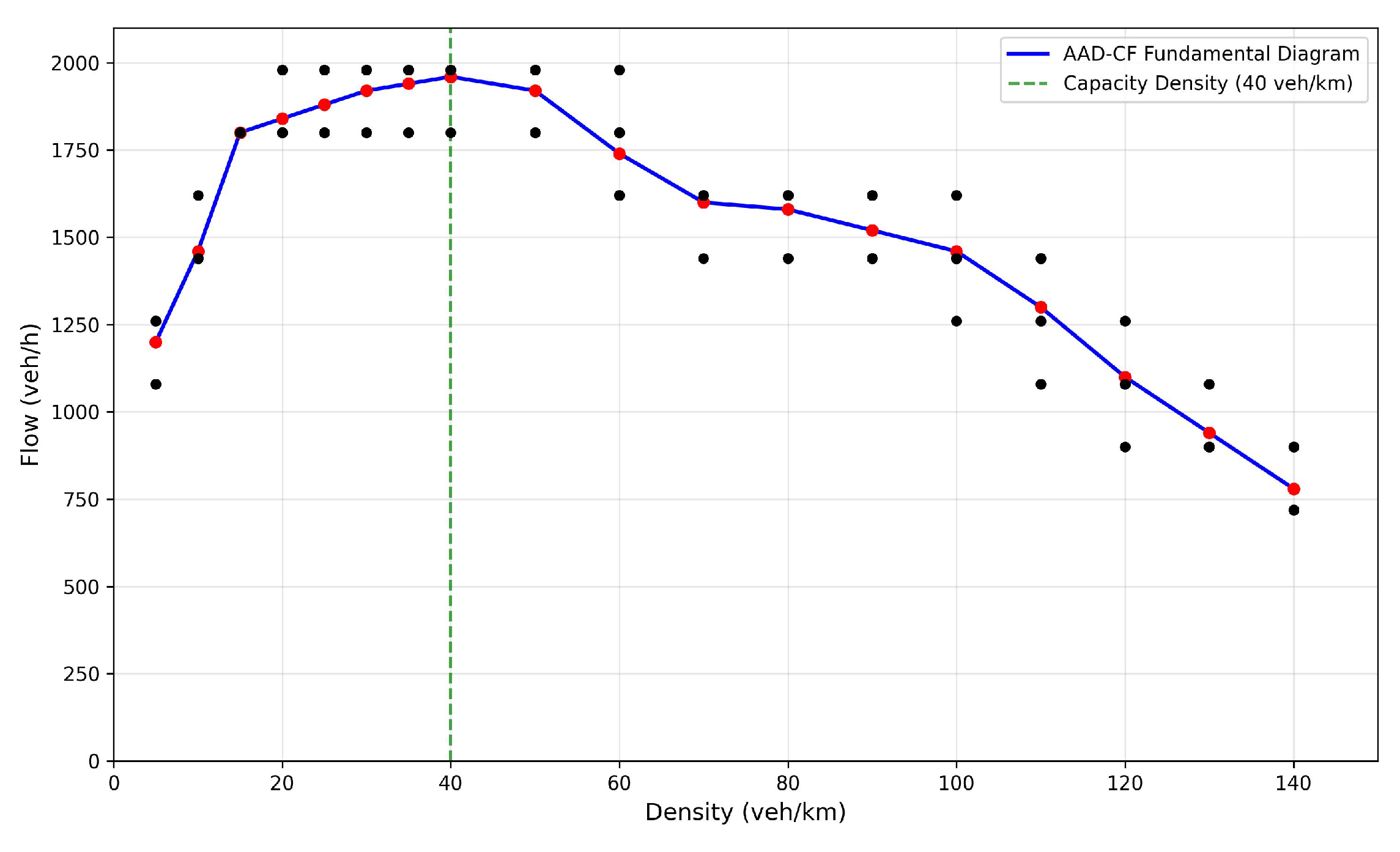
Furthermore, simulations were conducted with $N=5,10,15,20,25,30,35,40,50,60$. Traffic flow was collected at the 800 m section during t = 100–300 (s) using a 20 s time window. Each scenario yielded 10 flow measurements, whose averages were plotted as red dots to construct the flow–density relationship (Figure 7). Results show a vertically scattered distribution of flow at the same density, rather than a single curve, consistent with the three-phase traffic theory. The maximum flow, 1960 veh/h, occurred at a density of 40 veh/km.

These results demonstrate that the AAD-CF model maintains stability and adaptability under varying densities, particularly in sustaining synchronized flow at medium densities—an essential phenomenon that traditional two-phase models such as IDM fail to reproduce. The model’s advantage lies in the integration of asymmetric acceleration–deceleration behavior and a dual-tanh nonlinear adjustment mechanism, which significantly enhances its responsiveness and stability against disturbances.

In summary, combining microscopic trajectory fitting with macroscopic traffic flow simulations, the AAD-CF model not only achieves higher accuracy in reproducing individual driving behaviors but also shows superior capability in replicating three-phase traffic phenomena. This validates its applicability and advancement in modeling complex traffic systems.

6. Conclusions

This study focuses on the asymmetric phenomenon in acceleration and deceleration during car-following behavior and proposes an Asymmetric Acceleration and Deceleration Car-Following (AAD-CF) model. By establishing a dual-dimensional decision-making mechanism incorporating desired speed and spacing, and introducing an asymmetric correction factor, the model effectively captures differences in driving behavior. At the microscopic level, based on real-world trajectory data from the I-80 dataset, comparisons with benchmark models such as Gipps, IDM, and OVM show that AAD-CF model significantly reduces trajectory fitting errors across different simulation time steps (with an average RMSE reduction exceeding 10%), demonstrating higher simulation accuracy and robustness. At the macroscopic level, ring road simulations successfully reproduce three-phase traffic flow states and reveal an asymmetric characteristic where braking waves propagate approximately 40% faster than startup waves, validating the model’s effectiveness in bridging microscopic behavior and macroscopic phenomena.

The main contributions of this study lie in proposing an asymmetric correction factor with clear physical significance, providing a new method for quantifying differences in acceleration and deceleration behavior. Through multi-scenario validation, the model demonstrates advantages in both microscopic accuracy and macroscopic reproducibility, offering a new analytical tool for understanding the asymmetric propagation mechanisms of traffic waves. These results can provide model support for the development of traffic simulation systems and offer new perspectives for traffic flow theorists analyzing non-equilibrium traffic phenomena.

Future research will focus on introducing fuzzy control theory to extend desired state variables into fuzzy sets, establishing a fuzzy car-following model that accounts for drivers’ cognitive uncertainty. Additionally, lane-changing decision mechanisms will be integrated into multi-lane scenarios to enhance the model’s adaptability to various traffic conditions.

References

- Liu, C.; Liu, Z.; Chai, Y.; Liu, T. Review of Virtual Traffic Simulation and Its Applications. J. Adv. Transp. 2020, 1, 8237649. [Google Scholar] [CrossRef]
- Qi, X.; Ni, Y.; Xu, Y.; Tian, Y.; Wang, J.; Sun, J. Autonomous Vehicles’ Car-Following Drivability Evaluation Based on Driving Behavior Spectrum Reference Model. Transp. Res. Rec. J. Transp. Res. Board 2021, 2675, 129–141. [Google Scholar] [CrossRef]
- Shah, D.; Lee, C.; Kim, Y.H. Modified Gipps model: A collision-free car following model. J. Intell. Transp. Syst. 2023, 29, 18–31. [Google Scholar] [CrossRef]
- Awad, A.; Montasir, A. A Real-Time Safety-Based Optimal Velocity Model. Intell. Transp. Syst. 2022, 3, 165–175. [Google Scholar] [CrossRef]
- Zhang, C.; Sun, L. Bayesian Calibration of the Intelligent Driver Model. IEEE Trans. Intell. Transp. Syst. 2024, 25, 9308–9320. [Google Scholar] [CrossRef]
- Zheng, J.; Suzuki, K.; Fujita, M. Car-following behavior with instantaneous driver–vehicle reaction delay: A neural-network-based methodology. Transp. Res. Part C Emerg. Technol. 2013, 36, 339–351. [Google Scholar] [CrossRef]
- Cui, Z.; Wang, X.; Ci, Y.; Yang, C.; Yao, J. Modeling and analysis of car-following models incorporating multiple lead vehicles and acceleration information in heterogeneous traffic flow. Phys. A Stat. Mech. Its Appl. 2023, 630, 129259. [Google Scholar] [CrossRef]
- Ponnu, B.; Coifman, B. Speed-spacing dependency on relative speed from the adjacent lane: New insights for car following models. Transp. Res. Part B Methodol. 2015, 82, 74–90. [Google Scholar] [CrossRef]
- Ma, T.; Ahn, S. Comparisons of Speed-Spacing Relations under General Car following versus Lane Changing. Transp. Res. Rec. J. Transp. Res. Board 2008, 1, 138–147. [Google Scholar] [CrossRef]
- Siuhi, S.; Kaseko, M. Nonlinear acceleration and deceleration response behavior in stimulus-response car-following models. Adv. Transp. Stud. 2013, 31, 81–96. [Google Scholar] [CrossRef]
- Sun, J.; Zheng, Z.; Sun, J. Stability Evolution of Car-Following Models Considering Asymmetric Driving Behavior. Transp. Res. Rec. J. Transp. Res. Board 2023, 2677, 361–371. [Google Scholar] [CrossRef]
- Weng, J.; Zheng, Y.; Qu, X.; Yan, X. Development of a maximum likelihood regression tree-based model for predicting subway incident delay. Transp. Res. Part C Emerg. Technol. 2015, 57, 30–41. [Google Scholar] [CrossRef]
- Ren, X.; Chow, J.Y. A random-utility-consistent machine learning method to estimate agents’ joint activity scheduling choice from a ubiquitous data set. Transp. Res. Part B Methodol. 2022, 166, 396–418. [Google Scholar] [CrossRef]
- Gipps, P. A behavioural car-following model for computer simulation. Transp. Res. Part B Methodol. 1981, 15, 105–111. [Google Scholar] [CrossRef]
- Ting, S.; Lymburn, T.; Stemler, T.; Sun, Y.; Small, M. Parameter estimation for Gipps’ car following model in a Bayesian framework. Phys. A Stat. Mech. Its Appl. 2024, 639, 129671. [Google Scholar] [CrossRef]
- Newell, G.F. Operations Research. IEEE Open J. Intell. Transp. Syst. 1961, 9, 209–229. [Google Scholar] [CrossRef]
- Helbing, D.; Tilch, B. Generalized force model of traffic dynamics. Phys. Rev. E 1998, 58, 133–138. [Google Scholar] [CrossRef]
- Jiang, R.; Wu, Q.; Zhu, Z. Full velocity difference model for a car-following theory. Phys. Rev. E 2001, 64, 133–138. [Google Scholar] [CrossRef]
- Zhang, J.; Qi, H.; Zhang, Y. Two-Dimensional Intelligent Driver Model with Vehicular Dynamics. SAE Tech. Pap. 2022, 1, 7088. [Google Scholar] [CrossRef]
- Kerner, B.S. Three-phase traffic theory and highway capacity. Phys. A Stat. Mech. Its Appl. 2004, 333, 379–440. [Google Scholar] [CrossRef]
- Treiber, M.; Kesting, A.; Helbing, D. Three-phase traffic theory and two-phase models with a fundamental diagram in the light of empirical stylized facts. Transp. Res. Part B Methodol. 2010, 44, 983–1000. [Google Scholar] [CrossRef]
- Agarwal, A.; Rimal, A.; Ilunga, M. Non-linear Contact Analysis and Response Surface Optimization of Railway Wheel Using ANSYS. Math. Model. Eng. Probl. 2024, 11, 2039–2047. [Google Scholar] [CrossRef]
- Huang, X.; Sun, J.; Sun, J. Asymmetric driving behaviour analysis using field trajectories. WIT Trans. Built Environ. 2019, 186, 73–84. [Google Scholar] [CrossRef]
- Zhu, B.; Jiang, Y.; Zhao, J.; He, R.; Bian, N.; Deng, W. Typical-driving-style-oriented Personalized Adaptive Cruise Control design based on human driving data. Transp. Res. Part C Emerg. Technol. 2019, 100, 274–288. [Google Scholar] [CrossRef]
- Punzo, V.; Borzacchiello, M.T.; Ciuffo, B. On the assessment of vehicle trajectory data accuracy and application to the Next Generation SIMulation (NGSIM) program data. Transp. Res. Part C Emerg. Technol. 2011, 19, 1243–1262. [Google Scholar] [CrossRef]
- Montanino, M.; Punzo, V. Trajectory data reconstruction and simulation-based validation against macroscopic traffic patterns. Transp. Res. Part B Methodol. 2015, 80, 82–106. [Google Scholar] [CrossRef]