Automated Grading of Boiled Shrimp by Color Level Using Image Processing Techniques and Mask R-CNN with Feature Pyramid Networks

Featured Application

This study proposes an automated shrimp color grading system using image processing and deep learning; providing an objective and standardized method that enhances fairness and accuracy in shrimp quality assessment.

Abstract

Color grading of boiled shrimp is a critical factor influencing market price, yet the process is usually conducted visually by buyers such as middlemen and processing plants. This subjective practice raises concerns about accuracy, impartiality, and fairness, often resulting in disputes with farmers. To address this issue, this study proposes a standardized and automated grading approach based on image processing and artificial intelligence. The method requires only a photograph of boiled shrimp placed alongside a color grading ruler. The grading process involves two stages: segmentation of shrimp and ruler regions in the image, followed by color comparison. For segmentation, deep learning models based on Mask R-CNN with a Feature Pyramid Network backbone were employed. Four model configurations were tested, using ResNet and ResNeXt backbones with and without a Boundary Loss function. Results show that the ResNet + Boundary Loss model achieved the highest segmentation performance, with IoU scores of 91.2% for shrimp and 87.8% for the color ruler. In the grading step, color similarity was evaluated in the CIELAB color space by computing Euclidean distances in the L (lightness) and a (red–green) channels, which align closely with human perception of shrimp coloration. The system achieved grading accuracy comparable to human experts, with a mean absolute error of 1.2, demonstrating its potential to provide consistent, objective, and transparent shrimp quality assessment.

1. Introduction

The shrimp industry in Thailand currently faces challenges such as declining market prices due to internal and external factors. The domestic production of shrimp, including whiteleg shrimp (Litopenaeus vannamei) and black tiger shrimp (Penaeus monodon), has increased by 8.18% in 2023 compared to the previous year (Department of Fisheries 2023). Additionally, global shrimp production has surged, with significant contributions from countries like Ecuador, leading to an oversupply scenario. As a result, the industry must shift its focus toward enhancing product quality instead of product quantity to maintain profitability and stimulate consumption. One persistent issue hindering the improvement of shrimp quality in Thailand is the subjective and unfair color-based grading of boiled shrimp. Grading is typically performed visually by buyers, such as middlemen and processing plants, raising concerns about accuracy and impartiality. This lack of standardized grading often leads to disputes between buyers and farmers, as both parties have conflicting interests. Buyers may aim for lower grades to reduce costs, while sellers may expect higher grades to maximize revenue. The absence of a neutral color grading standard has demotivated farmers from improving the color quality of their shrimp.

The reddish-orange color on the surface of boiled shrimp is used as one of the quality indicators due to its acceptance by consumers, who prefer shrimp with vibrant colors [1]. Additionally, it serves as an indicator of shrimp health [2]. The orange color primarily originates from a carotenoid known as Astaxanthin (AST), a powerful antioxidant. This protein substance becomes visibly red when exposed to heat. AST is involved in various biological functions, including immune response, stress tolerance, and shrimp development. Consequently, boiled shrimp with a rich reddish hue is often more nutritionally valuable, particularly for their AST and pro-vitamin A content.

Factors that influence shrimp color include diet, environment, genetics, stress, pre-harvest handling, and storage processes. The pigments in shrimp, primarily AST, along with other carotenoids such as beta-carotene and lutein, are located in the exoskeleton and epidermis. Studies [3] indicate that supplementing shrimp diets with AST, either synthetic or natural sources such as Phaffia yeast, marigold flowers, and Haematococcus algae, significantly enhances immune responses. This improvement is evident through increased phagocytic activity, higher production of superoxide anions, and better resistance to Vibrio parahaemolyticus infections. Shrimp that receives AST supplements also exhibit a more intense color after cooking compared to those without supplementation [2].

Shrimp Grading Criteria in Thailand and other countries primarily consist of weight, freshness, and coloration. In Thailand, grades are often determined by weight in terms of the number of shrimps per kilogram (Count Per Kilogram or CPK) [4]. For example, medium-sized shrimp (M) correspond to 91–100 shrimp per kilogram. After weight-based grading, color grading is performed by comparing the shrimp’s color against reference color scales, such as ShrimpFan™ or SalmoFan™, using visual assessment [5]. The more intense the reddish-orange color, the higher and more valuable the grade. Color grades are identified by numbers or letters on the color reference, such as 20–34 or A1–A4. In traditional shrimp grading based on color in Thailand, graders must randomly select representative shrimps and visually compare their color with a reference color ruler. This process is challenging and prone to error because all colors fall within a similar tone range, making it difficult to accurately determine the closest matching color by eye. Human color perception is influenced by numerous factors, including background color and the illuminant’s color [6]. Moreover, if graders have a vested interest in the outcome, the reliability of the grading results is further reduced.

To let the computer vision has the same color differentiating perception like human’s eyes, The CIELAB color space (Lab) was invented [7]. It is designed to have a uniform color perception, meaning changes in color values correspond to equally perceptible changes to the human eye. Unlike RGB, where changes are non-uniform [8], CIELAB is more suitable for applications requiring accurate color differentiation for human perception.

To enable computer vision systems to approximate the perceptual characteristics of human color discrimination, the CIELAB color space was developed [7]. The fundamental objective of this color space is perceptual uniformity, meaning that numerical differences between colors correspond more closely to differences perceived by the human visual system [9]. This property distinguishes CIELAB from device-dependent models such as RGB, where variations in channel values do not scale uniformly with human perception, often leading to inconsistencies in color analysis [8]. The CIELAB model consists of three orthogonal axes: L*, representing lightness, and a* and b*, representing the green–red and blue–yellow opponent color dimensions, respectively. This design mirrors aspects of the human visual system’s opponent-process theory. Because of its perceptual uniformity, CIELAB has become a standard in fields where precise color measurement is required. CIELAB offers significant advantages over RGB by aligning computational color measurements with human visual assessment, ensuring both accuracy and interpretability.

Challenges in automated shrimp grading include overlapping issues such as morphological and color similarities among objects, which are often closely packed or overlapping (e.g., boiled shrimp and color reference scales in an image). These issues make segmenting and labeling objects in computer vision (defining which class each pixel belongs to and identifying the number for each object) more difficult. Instance segmentation, which is a deep learning method that integrates segmentation and object detection in a network, is a promising solution for those challenges since it uses a unified framework that allows the network to leverage shared features across tasks. Unlike separate networks that may suffer from fragmented learning, where segmentation focuses on pixel-level accuracy without instance differentiation, and labeling depends on post-processed outputs that might already include errors, instance segmentation jointly optimizes segmentation and detection, minimizing the propagation of intermediate errors. Shen et al. (2022) [10] demonstrated that a Mask R-CNN Feature Pyramid Networks (FPN) with a ResNet-50 as backbone effectively segmented grape bunches compared to other instance segmentation models. The Mask R-CNN model [11] extends Faster R-CNN by adding a branch for segmentation masks, enabling simultaneous object detection and segmentation. Key components include a backbone for feature extraction, a Region Proposal Network (RPN) for identifying regions of interest, ROI Align for reducing resizing losses, and a segmentation mask branch. Adding an FPN [12] to the backbone enhances the model’s ability to extract multi-scale features, particularly from images with objects of varying sizes.

To tackle fine-grained segmentations such as bicycle spokes, grape bunch, medical images, color grading bands, and shrimp legs, the boundary loss has been applied to emphasize precise boundary delineation by assigning different weights to the edges of foreground and background regions. This mechanism helps neural networks to better focus on areas where boundaries are thin, complex, or prone to ambiguity, improving the accuracy of segmentation in challenging scenarios. For instance, in the case of segmenting the left atrium in medical imaging [13], boundary loss ensures precise delineation of the atrium’s intricate structures, such as its thin walls and intersections with neighboring tissues. By assigning higher weights to critical boundary regions, the loss function guides the network to prioritize learning fine-grained details, effectively enhancing segmentation performance in tasks where accurate boundary detection is essential.

Efforts to develop automated shrimp grading methods have significantly increased in recent years, driven by two main factors: the demand for reducing manual labor in the seafood industry and the rapid advancement of computer vision, image processing, and artificial intelligence technologies [14]. Recently, Wang et al. (2023) [15] proposed a non-destructive system for assessing shrimp freshness using computer vision and artificial intelligence. In their system, shrimp are transported on a conveyor belt to capture images under predefined lighting and quality conditions. The system then grades shrimp freshness into four categories, with Grade 4 indicating substandard freshness. To build the classification model, the input data consisted of images of red shrimp alongside freshness levels determined by the total volatile basic nitrogen (TVB-N) measured at the time of imaging. Features were extracted using neural networks based on ResNet50 or Convolutional Neural Networks (CNNs), utilizing residual networks to mitigate the vanishing gradient problem. The network architecture was significantly enhanced with features such as dropout layers to encourage feature independence, the SiLU activation function combining the benefits of Sigmoid and ReLU, and replacing the Adam optimizer with Adagrad for better performance. The network’s final layer consisted of four neurons representing each freshness grade. Additionally, the system identified critical areas related to freshness through Grad-CAM, visualized as heatmaps where significant features appeared darker. The system achieved a classification accuracy of 98.29% on a test set of 1176 images.

Suárez et al. (2022) [16] introduced a shrimp grading method based on color, using photographs and artificial intelligence within CNN frameworks to automatically extract features from images. Their study used a database of side-view images of individual fresh L. vannamei, with the main goal of creating a smartphone-compatible application to classify shrimp into two grades. To meet the requirement for lightweight CNN architectures, they minimized the number of hidden layers, reducing the network’s depth and width while maintaining classification performance. They also implemented the Leaky ReLU activation function, which extends the possible value range from $0-\infty$ to $-\infty -\infty$, preserving output diversity and enhancing learning continuity in simpler networks. For color representation, HSV was chosen over RGB for its better differentiation and smaller size due to the separation of intensity from color information. The binary classifier was trained on a labeled dataset of 800 images annotated by experts and achieved an average classification accuracy of 97.7% on a test set of 300 images.

Poonnoy et al. (2014) [17] developed a computer vision system to automatically classify the sizes of boiled shrimp. Their approach utilized Relative Internal Distance (RID) as a morphological feature to quantify differences in shrimp shapes, which were automatically extracted from photographs. The process began with obtaining binary images of shrimp, identifying boundary lines on the top and bottom sides, and calculating a central axis between them. RID was defined as the ratio of shrimp length to the shortest distance between 62 predefined contour points along the top and bottom boundaries. This feature was input into a neural network with a single hidden layer of 15 nodes. The final layer classified the shrimp images, achieving an average accuracy of 99.8% for boiled L. vannamei.

In sum, most research on automated shrimp grading has focused on size classification, with limited studies exploring color-based grading. However, these works still remain insufficient for practical use due to incomplete automation in certain processes, excessive environmental constraints, and the limited number of grades, which do not align with the needs of shrimp trading in Thailand.

2. Materials and Methods

2.1. Data Collection

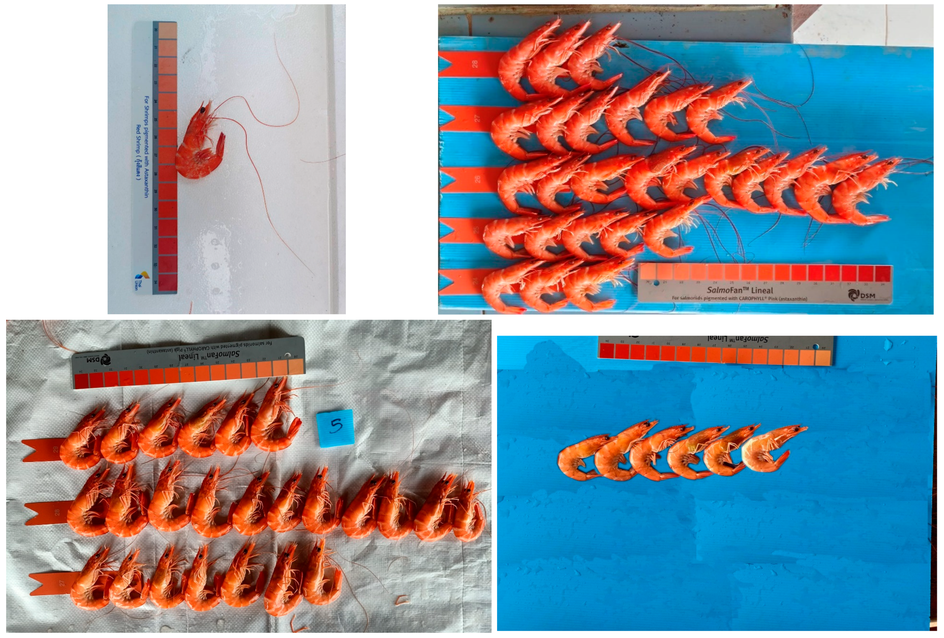
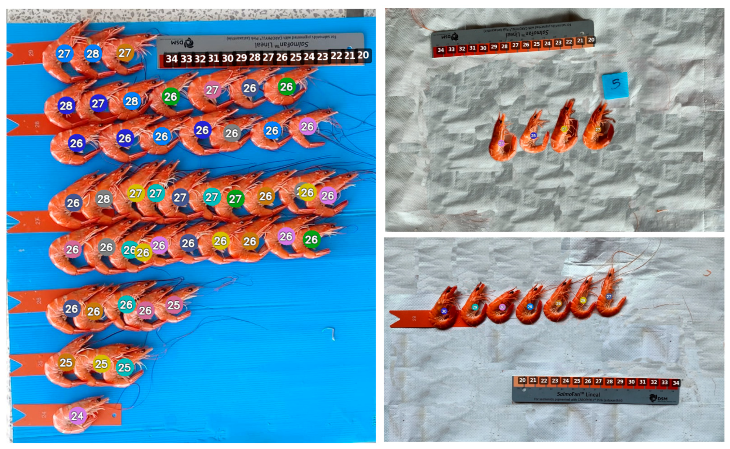
The photographs used as the dataset for this study were collected from two Thai provinces, Surat Thani and Nonthaburi. They consist of images of boiled L. vannamei taken during the grading process. Live shrimp were boiled in water at 100 °C for 15 min before being placed on a table alongside color grading rulers of Thai Union Hatchery Co., Ltd., Mueang Samut Sakhon, Thailand and SalmoFan™, Basel, Switzerland. Three experts independently assigned color grades to each specimen. Thereafter, images were acquired under ambient illumination of 80–120 lux, typical of indoor ceiling lighting, as measured with an STMicroelectronics VL53L0X light sensor, and photographs were captured using a smartphone-mounted digital camera (12.2 MP, 4032 × 3024 px) (as shown in Figure 1). The images were compressed using the Joint Photographic Experts Group (JPEG) format. The number of shrimp per image ranged from 1 to 52. This resulted in a dataset of 800 photographs of boiled L. vannamei, of which 200 were from Nonthaburi Province.

2.2. Dataset Augmentation

To enable artificial intelligence to handle input images with varying characteristics, including resolution, brightness, and angles, the collected dataset of boiled L. vannamei images was resized to 512 × 512 pixels and augmented using various image processing techniques as follows:

• Image Rotation:

The images were rotated by an angle $\theta$ (in degrees), where $\theta$ is randomly selected from the range $-30$ to $30$.

$$\left[{\displaystyle \genfrac{}{}{0pt}{}{x^{\prime }}{y^{\prime }}}\right]=\left[{\displaystyle \genfrac{}{}{0pt}{}{\mathit{cos}\theta -\mathit{sin}\theta }{\mathit{sin}\theta \mathit{cos}\theta }}\right]\left[{\displaystyle \genfrac{}{}{0pt}{}{x-x_c}{y-y_c}}\right]+\left[{\displaystyle \genfrac{}{}{0pt}{}{x_c}{y_c}}\right]$$

(1)

$x,y$ denoted pixel coordinates in the original image, $x^{\prime },y^{\prime }$ denoted pixel coordinates after rotation. $\theta =$ rotation angle in radians $={\displaystyle \frac{{\theta }_{deg}\pi }{180}}$, $x_c,y_c$ are center of rotation (in this research, the image center).

• Adding Gaussian Noise:

$$I^{\prime }\left(x,y\right)=I\left(x,y\right)+N(x,y)$$

(2)

Gaussian noise was added to simulate image imperfections. The pixel intensity values before and after noise addition are represented as $I\left(x,y\right)$ and $I^{\prime }(x,y)$, respectively.

$N\left(x,y\right)~N(0,{\sigma }^2)$ is the Gaussian noise function, and $\sigma$ is the noise level defined as:

$(\sim \mathrm{U}\mathrm{n}\mathrm{i}\mathrm{f}\mathrm{o}\mathrm{r}\mathrm{m}(0,\mathrm{m}\mathrm{a}\mathrm{x}\_\mathrm{n}\mathrm{o}\mathrm{i}\mathrm{s}\mathrm{e}\left)\right)\times 255$ ($\mathrm{m}\mathrm{a}\mathrm{x}\_\mathrm{n}\mathrm{o}\mathrm{i}\mathrm{s}\mathrm{e}$ = 0.05 for this research).

• Brightness Adjustment:

$$I^{″}\left(x,y\right)=I^{\prime }(x,y)\times \beta$$

(3)

The brightness of the images was adjusted by multiplying the pixel intensity with a brightness factor $\beta$, defined as: $\beta =\sim Uniform(\beta min,\beta max)$. For this research, $\beta min$ = 0.8, $\beta max$ = 1.2.

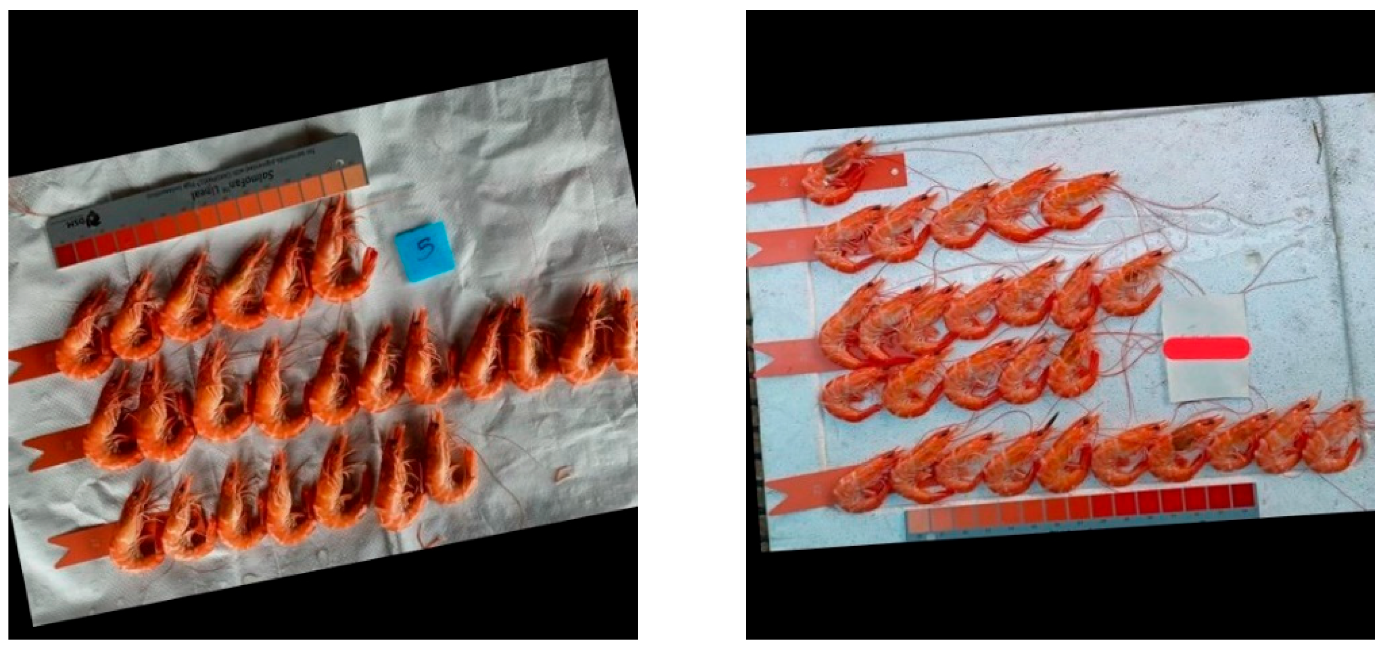
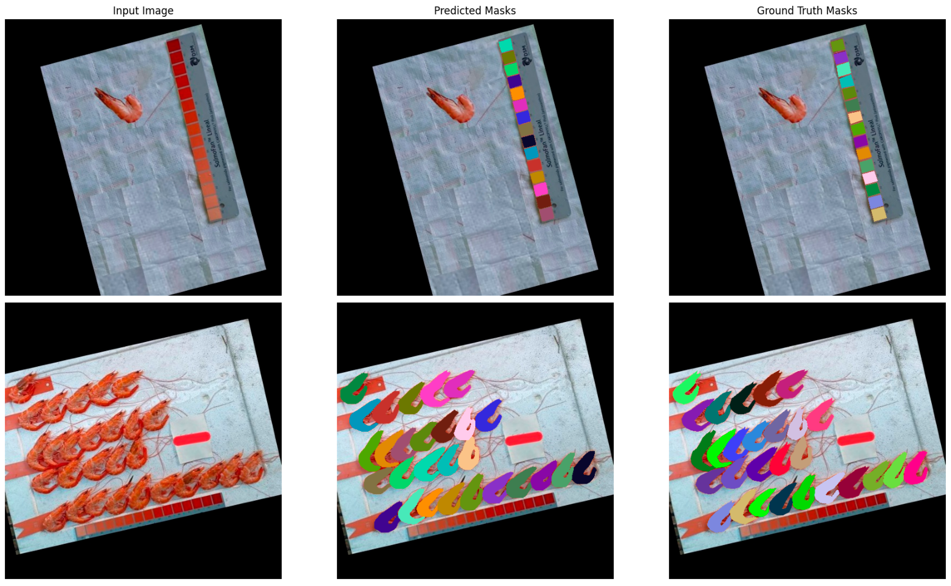
After augmentation, the dataset was increased threefold, resulting in a total of 2400 images. Examples of images in the dataset are shown in Figure 2.

2.3. Image Annotation Creation

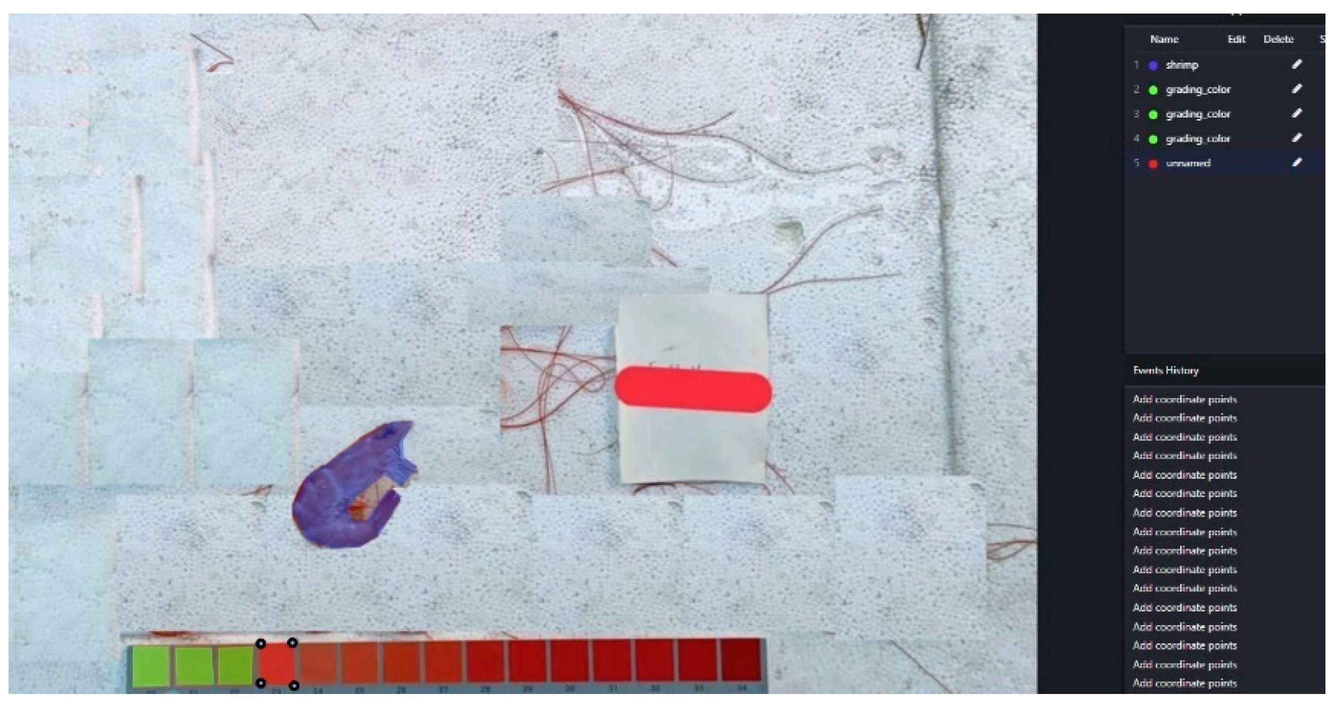
The process of creating image annotations, or ground truth, for segmentation tasks enables artificial intelligence to identify areas corresponding to boiled shrimp, color grading bands in the ruler, and the background. During this phase, the ground truth is manually labeled in the shape of polygons by humans using PixLab annotation generator (annotate.pixlab.io, accessed on 20 August 2025). Annotations must be generated for all original images (800 in total), as illustrated in Figure 3.

2.4. Deep Learning Networks for Instance Segmentation

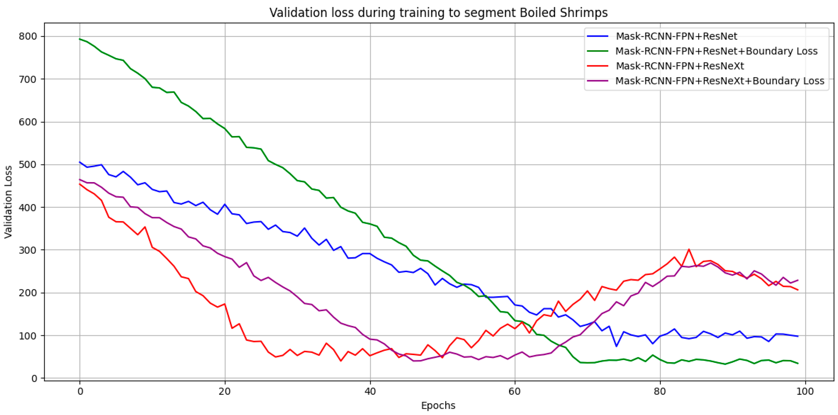
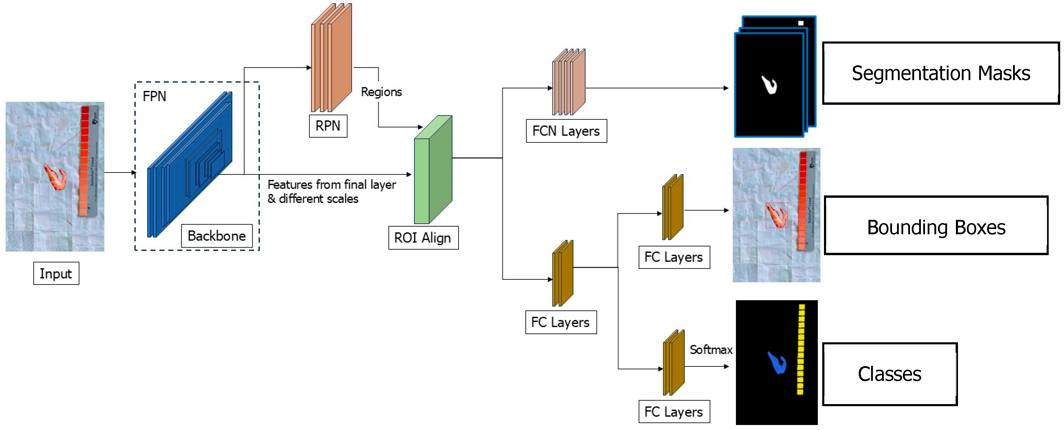
In this research, we utilized a state-of-the-art deep learning network architecture for instance segmentation, Mask-RCNN-FPN [11], with two different backbone networks, ResNeXt [18] and ResNet [19], to do both segmentation and detection of the shrimps and color grading bands in the image. This architecture consists of five parts, and can be seen in Figure 4. FC denotes Fully Connected and FCN denotes Fully Connected Network.

2.4.1. Backbone Network

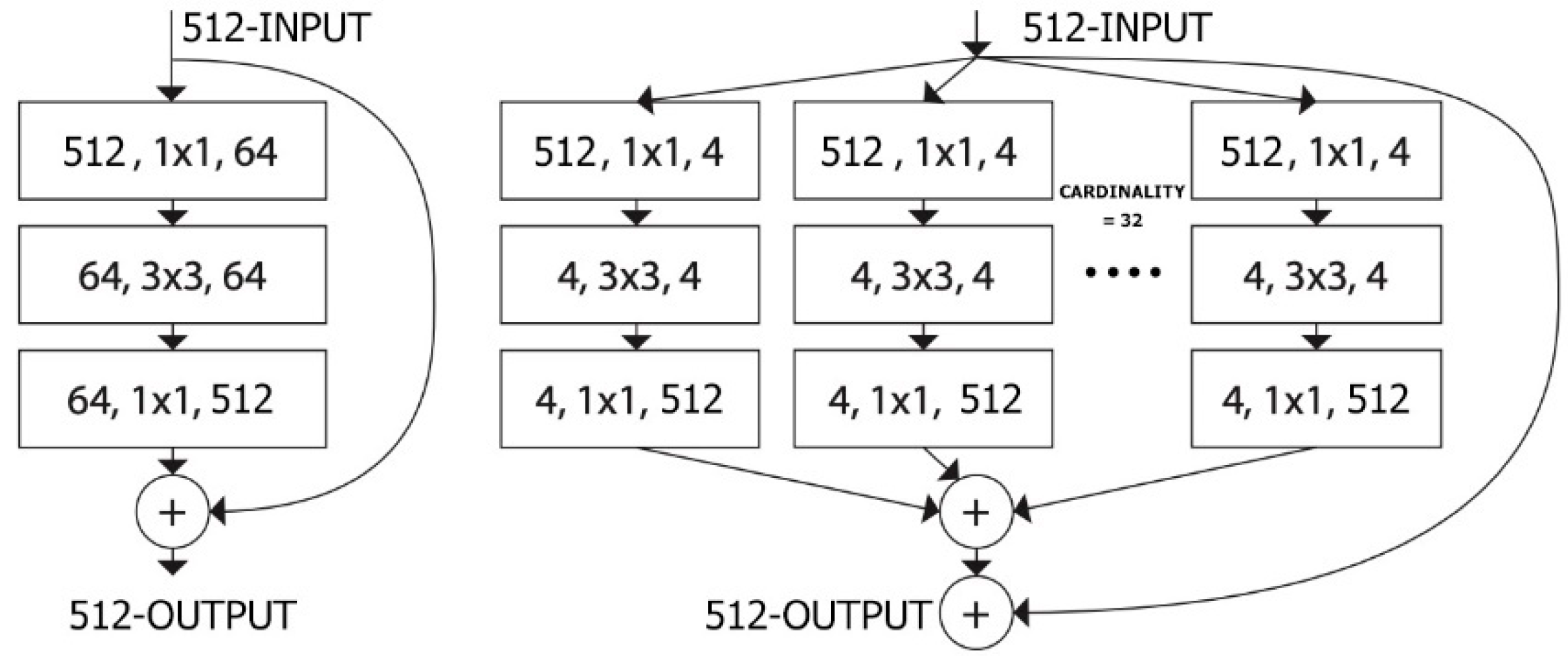
Backbone network serves as the feature extractor, responsible for transforming the input image into high-dimensional feature maps that capture essential information such as edges, textures, and object parts. In this research, either ResNet or ResNeXt is utilized as a backbone and enhanced with an FPN to handle objects of varying sizes by constructing a multi-scale feature representation. The FPN achieves this by combining feature maps from different levels of the backbone in a top-down manner, augmenting low-resolution, high-semantic features with high-resolution, low-semantic ones. This hierarchical representation ensures that both small and large objects are effectively captured. Both ResNet and ResNeXt architectures (as shown in Figure 5) are CNNs that utilize residual connections directly passing input information to subsequent layers to mitigate the vanishing gradient problem in complex learning scenarios. However, they differ in that ResNeXt introduces an additional dimension through the concept of cardinality, which involves adding groups of parallel convolutional layers. This design extracts more diverse features from the input data without significantly increasing computational overhead. This enhancement improves object segmentation performance, particularly for objects with similar shapes or colors, though it also carries an increased risk of overfitting. Hence, we need to test it both to find a better backbone for this challenging segmentation task.

The detailed structure of FPN can be shown as the Algorithm 1.

Algorithm 1. FeaturePyramidNetwork

(fpn): FeaturePyramidNetwork(  (inner_blocks): ModuleList(    (0): Conv2dNormActivation(      (0): Conv2d(256, 256, kernel_size=(1, 1), stride=(1, 1))    )    (1): Conv2dNormActivation(      (0): Conv2d(512, 256, kernel_size=(1, 1), stride=(1, 1))    )    (2): Conv2dNormActivation(      (0): Conv2d(1024, 256, kernel_size=(1, 1), stride=(1, 1))    )    (3): Conv2dNormActivation(      (0): Conv2d(2048, 256, kernel_size=(1, 1), stride=(1, 1))    )  )  (layer_blocks): ModuleList(    (0-3): 4 x Conv2dNormActivation(      (0): Conv2d(256, 256, kernel_size=(3, 3), stride=(1, 1), padding=(1, 1))    )  )  (extra_blocks): LastLevelMaxPool()   )

2.4.2. Region Proposal Network (RPN)

The RPN generates candidate regions of interest (ROIs) that are likely to contain objects. It operates on the feature maps produced by the backbone and slides over them with predefined anchor boxes of various scales and aspect ratios. For each anchor, the RPN predicts an objectness score (object or background) and regresses the anchor box coordinates to better fit the object. The ROIs are filtered using a non-maximum suppression (NMS) process to remove redundant proposals. The detailed structure of the RPN can be shown as the Algorithm 2.

Algorithm 2. RegionProposalNetwork

(RPN): RegionProposalNetwork(    (anchor_generator): AnchorGenerator()    (head): RPNHead(    (conv): Sequential(     (0): Conv2dNormActivation(       (0): Conv2d(256, 256, kernel_size=(3, 3), stride=(1, 1), padding=(1, 1))       (1): ReLU(inplace=True)     )    )    (cls_logits): Conv2d(256, 3, kernel_size=(1, 1), stride=(1, 1))    (bbox_pred): Conv2d(256, 12, kernel_size=(1, 1), stride=(1, 1))    )   )

2.4.3. Roi Align

Once the ROIs are identified, they are refined and resized using ROI Align to ensure that the feature maps align accurately with the proposed regions. Unlike traditional ROI Pooling, which rounds ROI boundaries to the nearest pixel, ROI Align uses bilinear interpolation to maintain spatial accuracy. This step ensures that the extracted features for each ROI are precise, which is crucial for the task where objects are prone to touch or overlap like shrimps on production line.

2.4.4. Classes and Bounding Box

The refined ROIs are passed through FC layers to predict class labels (for this research: shrimp, color grading band, background) and further refine the bounding box coordinates. The classifier assigns each ROI to a specific class, while the regression head adjusts the bounding box to better encompass the object. The detailed structure can be shown as the Algorithm 3, cls denoted classes and bbox denoted bounding box.

Algorithm 3. Classes and Bounding Box

(roi_heads): RoIHeads(  (box_roi_pool): MultiScaleRoIAlign(featmap_names=[‘0’, ‘1’, ‘2’, ‘3’], output_size=(7, 7), sampling_ratio=2)  (box_head): TwoMLPHead(    (fc6): Linear(in_features=12544, out_features=1024, bias=True)    (fc7): Linear(in_features=1024, out_features=1024, bias=True)  )  (box_predictor): FastRCNNPredictor(    (cls_score): Linear(in_features=1024, out_features=2, bias=True)    (bbox_pred): Linear(in_features=1024, out_features=8, bias=True)  ) )

2.4.5. Segmentation

The segmentation part is FCN that operates in parallel with the classification and bounding box regression heads. For each ROI, it predicts a binary mask at the pixel level, indicating the presence of the object within that ROI. Each class has its own dedicated mask, and only the mask corresponding to the predicted class is used. This process provides the instance segmentation capability of Mask R-CNN, allowing it to delineate individual objects with pixel-level accuracy. The detailed structure of segmentation part can be shown as the Algorithm 4.

Algorithm 4. Segmentation

(roi_heads): RoIHeads( (mask_roi_pool): MultiScaleRoIAlign(featmap_names=[‘0’, ‘1’, ‘2’, ‘3’], output_size=(14, 14), sampling_ratio=2)  (mask_head): MaskRCNNHeads(    (0): Conv2dNormActivation(     (0): Conv2d(256, 256, kernel_size=(3, 3), stride=(1, 1), padding=(1, 1))     (1): ReLU(inplace=True)    )    (1): Conv2dNormActivation(     (0): Conv2d(256, 256, kernel_size=(3, 3), stride=(1, 1), padding=(1, 1))     (1): ReLU(inplace=True)    )    (2): Conv2dNormActivation(     (0): Conv2d(256, 256, kernel_size=(3, 3), stride=(1, 1), padding=(1, 1))     (1): ReLU(inplace=True)    )    (3): Conv2dNormActivation(     (0): Conv2d(256, 256, kernel_size=(3, 3), stride=(1, 1), padding=(1, 1))     (1): ReLU(inplace=True)    )  )  (mask_predictor): MaskRCNNPredictor(    (conv5_mask): ConvTranspose2d(256, 256, kernel_size=(2, 2), stride=(2, 2))    (relu): ReLU(inplace=True)    (mask_fcn_logits): Conv2d(256, 2, kernel_size=(1, 1), stride=(1, 1))  ) )

2.5. Loss Functions

This research employs two loss functions: standard loss and boundary loss. These loss functions will be used independently to identify the better-performing approach and the most suitable network architecture for each. The standard loss function focuses on measuring the overlap or similarity between the predicted segmentation mask and the ground truth. It typically incorporates Cross-Entropy Loss, which is region-based and primarily evaluates pixel-wise classification accuracy but may not adequately emphasize boundary details. The standard loss can be computed as the following:

$$L_{std}=L_{cls}+L_{reg}+L_{mask}+L_{obj}$$

(4)

$L_{cls}$: Classification loss, $L_{reg}$: Bounding box regression loss, $L_{mask}$: Mask segmentation loss, $L_{obj}$: Object detection loss.

Boundary loss is calculated based on the distance of each pixel from the object’s boundary, with pixels closer to the boundary contributing more to the loss than those further away. This unequal weighting mechanism helps the network learn to define object boundaries with greater precision. In this research, segmentation errors near object boundaries have a significantly greater impact than errors in other areas, as the objects often have very close boundaries (as shown in Figure 1). If segmentation fails to separate the boundaries of individual objects, it can lead to detection errors, such as merging multiple color grades into one or assigning the wrong color grade to a shrimp. The boundary loss can be computed as the following:

$$L_{boundary}=\sum _i{d}_i·\left|p_i-g_i\right|$$

(5)

Let $d_i$ denoted the distance between pixel $i$ and the boundary in the distance map, and $p_i,g_i$ denoted the predicted value and the ground truth value at pixel $i$, respectively.

$$L_{total}=L_{std}+L_{boundary}$$

(6)

In summary, there would be 2 approaches, using $L_{std}$ alone and using $L_{total}$ which incorporates the boundary loss.

2.6. Optimizer and Regularization

In this research we use the Adam optimizer with an explicit L₂ regularization (weight decay) term to improve generalization and mitigate over-fitting. Concretely, at each update step, the loss is minimized.

$$L+{\displaystyle \frac{\mathsf{\lambda }}{2}}‖\theta ‖{\displaystyle \genfrac{}{}{0pt}{}{2}{2}}$$

(7)

where $L$ in this research is either $L_{total}$ or $L_{std}$, $\mathsf{\lambda }$ is the weight decay coefficient, set to ${10}^{-5}$, and $\mathsf{\lambda }$.

For Adam update rule, all trainable parameters, $\theta$, in the network are updated using a combination of the first moment estimate (mean of gradients) and the second moment estimate (variance of gradients). The update rule for each parameter at step $t$ is given as the following:

$${\theta }_{t+1}={\theta }_t-{\displaystyle \frac{\eta }{\sqrt{{\widehat{v}}_t+ϵ}}}{\widehat{m}}_t$$

(8)

where ${\widehat{m}}_t$ and ${\widehat{v}}_t$ denote the bias-corrected first and second moment estimates, respectively. $\eta$ is the learning rate (for this research, 0.001), and $ϵ$ is a small constant to prevent division by zero.

We incorporate L₂ regularization by adding a penalty term ${\displaystyle \frac{\lambda }{2}}‖{\theta ‖}_2^2$ to the loss, which yields an extra $\mathsf{\lambda }{\theta }_{t-1}$ term in the gradient. The resulting update becomes.

$${\theta }_t={\theta }_{t-1}-\eta \left({\displaystyle \frac{{\widehat{m}}_t}{\sqrt{{\widehat{v}}_t+ϵ}}}+\mathsf{\lambda }{\theta }_{t-1}\right)$$

(9)

2.7. Representative Color Identification and Distance Measurement for Boiled Shrimp Color Grading

This research focuses on classifying the colors of boiled shrimp to assign appropriate grades for buyers and shrimp farmers. We selected the CIELAB (Lab) color space (Müller et al., 2024) [7] due to its perceptual uniformity, closely resembling human color perception. The representative color of each boiled shrimp and each grading color band was calculated as the average color across all pixels. The representative color of a shrimp was then compared with the representative colors of all grading bands in the image by measuring the distance, identifying the color band closest to the shrimp as its grade.

$$\begin{array}{c}{L}_{diff}=\left|L_s-L_c\right|\hspace{1em}{a}_{diff}=\left|a_s-a_c\right|\\ dist=L_{diff}+a_{diff}\end{array}$$

(10)

Let $L_s,L_c$ denote the average lightness of the shrimp and the grading band.$a_s,a_c$ denote the average red-green chromatic values of the shrimp and the grading band, and $dist$ denotes the distance between colors in the CIELAB color space.

The distance calculation considers only two dimensions: lightness ($L$) and red-green chromaticity ($a$) while blue–yellow chromaticity ($b$) is excluded because it introduces noise from mis-segmented/background pixels and indoor lighting casts that are not informative for redness in this task. This design choice is consistent with prior redness quantification work that measures $a$ (and $\Delta a$) in CIELAB without using $b$. After comparing the shrimp’s representative color with all 15 grading bands in the image (Figure 6), the band with the smallest distance is selected as the shrimp’s color grade. The grade number (20–34) is then determined by the position of the identified band together with the intensity of the red color; if the first-ranked band has higher red intensity than the last-ranked band, the order is reversed. In our ablation, adding $b$ (i.e., using a 3D $Lab$ distance) reduced accuracy and increased variance across folds, so we retain the $La$ formulation for the remainder of this research.

2.8. Segmentation and Grading Performance Metrics

The performance of shrimp and color grading band segmentations is evaluated using the Intersection over Union (IoU) metric. IoU is particularly suited for this research because it addresses class imbalance, a significant challenge in this problem where the majority of the image consists of background pixels, and the regions of interest (shrimp and grading bands) occupy only a small fraction of the image. The predicted masks of shrimps and grading band from the segmentation part in the Mask-RCNN and the ground truth in the form of binary images were used to calculate the IoU as the following:

$$IoU=\left|{\displaystyle \frac{A\cap B}{A\cup B}}\right|$$

(11)

where $A$ denotes the predicted segmentation mask, and $B$ denotes the ground truth mask. This metric ensures a balanced evaluation by considering both false positives (over-segmentation) and false negatives (under-segmentation), making it robust for cases where one class (e.g., background) dominates the image.

In terms of color grading, we use the Mean Absolute Error (MAE) to define the difference between the predicted color grade and the color grade the experts provided visually. The range of possible grades is 20–34 (as shown in the ruler).

$$MAE={\displaystyle \frac{1}{n}}{\sum }_{i=1}^n\left|y_i-{\widehat{y}}_i\right|$$

(12)

$y_i$ denotes the grade provided by the experts, ${\widehat{y}}_i$ denotes the predicted grade, and $n$, the total number of shrimps.

3. Results

Segmentation Results

The dataset contained 2400 images. We first reserved 480 images (20%) as an untouched test set. The remaining 1920 images were used for model selection via 10-fold cross-validation: in each fold, approximately 1728 images were used for training and 192 for validation. Each fold was trained for up to 10 epochs, and within each fold the checkpoint with the lowest validation loss was retained as the best model. All models were trained to segment shrimp and the color-grading band separately to reduce error accumulation from learning multiple classes at once. The network received 512 × 512-pixel images and produced instance masks equal to the number of detected objects (see Figure 7).

Predicted and ground-truth masks were assigned different colors for visualization and were compared using Intersection-over-Union (IoU). The losses after 100 epochs are shown in Figure 8 and Figure 9.

The training losses indicate signs of overfitting for both Mask-RCNN-FPN + ResNeXt, with and without Boundary Loss, in the shrimp task, and for Mask-RCNN-FPN + ResNeXt in the color grading band task. These signs become apparent around epoch 37 for the color grading band task and epoch 25 for the shrimp task, as the loss begins to increase after an initial decline. As discussed in Section 2.4.1, the highly sophisticated architecture of ResNeXt could result in this behavior. Figure 10 was a result of using the weight from the last epoch of an overfitting model. As can be seen, many orange-red pixels were mistaken as color grading bands. Notably, Mask-RCNN-FPN + ResNeXt + Boundary Loss achieved the lowest loss for the color-grading-band task (3.19), followed by Mask-RCNN-FPN + ResNet + Boundary Loss (3.60). For the shrimp-segmentation task, Mask-RCNN-FPN + ResNet + Boundary Loss achieved the lowest loss (2.94), with Mask-RCNN-FPN + ResNeXt + Boundary Loss second (11.21).

In terms of validation loss, Mask-RCNN-FPN + ResNet + Boundary still remains the most promising model, achieving 16.5 for the color grading band task and 32.4 for the shrimp task. These results provide evidence that Boundary Loss enhances accuracy for fine-grained segmentation tasks. After training, once the networks have learned to detect shrimps, color grading bands, and generate masks, the best parameter set of each model based on validation loss will be evaluated on the testing set. The model with the highest IoU will then be selected.

From

Table 1. Performance of all models with their best parameter sets over 100 epochs for segmenting objects in images.

Models	IoU (%) Between Predicted Masks and Ground Truths
	Shrimp	Color Grading Band
Mask-RCNN-FPN + ResNet	90.0	84.1
Mask-RCNN-FPN + ResNet + Boundary loss	91.2	87.8
Mask-RCNN-FPN + ResNeXt	76.8	80.9
Mask-RCNN-FPN + ResNeXt + Boundary loss	88.4	86.4

, it can be seen that Boundary Loss improves IoU by approximately 2.4% for ResNet and 8.5% for ResNeXt. The best performance for both tasks is achieved by Mask-RCNN-FPN + ResNet + Boundary Loss, making it the sole model used for object segmentation and detection in this research. These results are proof that less sophisticated networks like ResNet can sometimes outperform more advanced architectures like ResNeXt due to their simplicity and better generalization. ResNeXt, with its highly sophisticated architecture and increased parameters, is more prone to overfitting, which hinders its performance on unseen data. On the other hand, ResNet’s simpler design can effectively capture essential patterns without overfitting, making it a more robust choice.

Subsequently, 800 photographs of shrimp, each shrimp assigned a color grade by experts, are segmented to determine the representative CIELAB colors. The segmented color grading band with the closest $L$ and $a$ channel values to the shrimp is assigned as the color grade for that shrimp. The mean absolute error (MAE) between the expert-assigned grades and the automated color grading is 1.2. The result of the automated color grading was shown in Figure 11.

This automated shrimp color-grading system can produce 15 color grades and requires only the inclusion of a grading ruler in the photo. Photos can be captured under normal indoor building lighting; no controlled conditions are necessary. The approach is practical for buyers and sellers: grading can be performed objectively using just a mobile phone and the ruler. Agreement with expert judgment is close (MAE = 1.2); for example, if an expert assigns grade 27, the system typically predicts within ±1 (e.g., 26 or 28).

4. Conclusions

This research presents a new approach to automating the color grading of boiled shrimp using image processing and Mask-RCNN with Feature Pyramid Networks. By combining advanced segmentation techniques with the CIELAB color space for representative color identification, the proposed method achieves precise segmentation and color grading comparable to expert judgments, with a mean absolute error (MAE) of 1.2. Notably, the use of Boundary Loss enhances segmentation accuracy, achieving an IoU of 91.2% for shrimp and 87.8% for color grading bands. Among the tested models, Mask-RCNN-FPN + ResNet + Boundary Loss emerged as the most robust and reliable architecture for segmenting both shrimp and color grading bands.

Unlike prior methods that require static environmental conditions and provide limited color grades, this research offers a more practical solution capable of delivering 15 color grades (equivalent to the current Thai shrimp color grading) with minimal additional requirements, only a grading ruler and a mobile phone. This advancement ensures fairness and precision in shrimp grading, enabling buyers and sellers to evaluate shrimp quality more impartially and efficiently. The findings underscore the potential of combining deep learning and image processing to address challenges in seafood grading, paving the way for further applications in the food industry. Future work may focus on developing a new approach that eliminates the need for a grading ruler, using only photographs of shrimp while maintaining accuracy.

We have deployed our boiled shrimp color grading system as a LINE chatbot, accessible by scanning the following QR code.