Abstract
This article presents a comparison between a classical PID controller and a fractional-order PID (FOPID) controller for a gyroscope with Cardan suspension (3 DOF). A gyroscope dynamics model accounting for gyroscopic couplings and viscous damping is adopted, while the FOPID controller is implemented in discrete form using the Grünwald–Letnikov (GL) operator, which reduces smoothly to the classical PID when λ = μ = 1. The effectiveness of both strategies is assessed in a moving-target tracking task using the IAE (tracking accuracy) and ISC (control effort) indices. MATLAB/Simulink R2025a simulations (ode4, Δt = 2 × 10⁻⁴ s) show that, under cross-axis couplings of the gyroscope suspension, FOPID yields smaller tracking errors and smoother control signals than PID. The results indicate the usefulness of fractional-order controllers in gyroscope control systems and provide a basis for further experimental studies.
1. Introduction
The problem of gyroscope motion—a rotating, symmetric rigid body—belongs to the key topics of classical theoretical mechanics. Its significance follows from the numerous applications of gyroscopes across scientific disciplines and engineering practice. The mathematical foundations describing gyroscope dynamics were formulated in the 18th century by L. Euler and subsequently developed by Lagrange, D’Alembert, and Laplace. Practical implementation is owed to Foucault, who constructed a device with a rapidly rotating axially symmetric body mounted in a Cardan joint. With the development of industry came advances in theoretical models of the gyroscope and progress in their technical applications.
At present, the issues of gyroscopic motion continue to attract the interest of many researchers. Scarborough [1] analyzes gyroscopic phenomena from the perspective of kinetic energy behavior and changes in the angular momentum of a rotating rotor. In turn, publications [2,3,4,5,6,7] contain an analysis of the dynamics of gyroscopes placed on vibrating bases, accounting for both linear and nonlinear damping and for external disturbances. To control chaotic behavior and to synchronize two gyroscopes, a range of control methods has been employed, including adaptive algorithms [2], active control [3], fuzzy logic [4], sliding-mode control [5], as well as fuzzy sliding-mode and adaptive sliding-mode control [6,7].
In modern industry, MEMS and optical gyroscopes play a dominant role, mainly used as angular-velocity sensors. Nevertheless, classical mechatronic gyroscopes are still used, e.g., in aviation and navigation systems, as drives in target-tracking coordinators for guided missiles, in spacecraft control systems, and in autonomous space-scanning systems [8]. When set into rotary motion, the mechatronic gyroscope rotor maintains the orientation of its axis, exhibiting only slight precession. This property makes gyroscopes indispensable components of control and navigation devices.
Today, research focuses on modern control methods for Cardan-suspension gyroscopes. The authors of [9] proposed using multiple gyroscopes as vibration dampers in wind- and earthquake-loaded towers. In [10], four controllers were examined for a scan-and-track gyroscope: a classical PD with optimal parameters, fuzzy PD and PID, and an adaptive fuzzy controller. Article [11] presents a control architecture combining backstepping with a nonlinear disturbance observer for a double-gimbal control-moment gyro, in the presence of various disturbances. In [12], model-predictive control (MPC) laws were developed for a DGSPCMG (double-gimbal scissored-pair control-moment gyro), with gimbal angle and rate limits. Publication [13] addressed singularity avoidance in a four-SGCMG cluster, proposing an innovative solution—adding a stepper motor to rotate the entire cluster—and comparing it with a VSCMG-based approach.
Currently, to achieve reliable performance, fractional-order controllers are widely used by many researchers [14,15]. The fractional-order PID (FOPID) controller was introduced by Podlubny, I [16]. The foundations for using fractional-order controllers were presented in [17]; tuning rules for FOPID appear, among others, in [18,19], while application examples can be found in [20,21].
The authors of the present study, in article [22], presented an analytical solution to the system of equations of motion of a gyroscope suspended on a Cardan joint, together with the initial conditions adopted for computation. This enabled closed-form relations describing the time evolution of the gyroscope-axis tilt and deviation angles. The resulting expressions were compared with numerical results obtained using the conventional fourth-order Runge–Kutta method. The proposed solution is accurate and universal, independent of the control moments.
Extending the state of the art, we present the use of a fractional-order PID controller to control a gyroscope with a gimbal suspension, often employed as a drive in guidance/target-tracking systems. A fractional PID is an extension of the classical controller; it is less sensitive to changes in both the plant parameters and the controller itself. Moreover, a fractional controller can readily achieve the iso-damping property [14].
This article is organized as follows: first, we present the structures of the classical PID and the fractional-order PID controllers, along with the mathematical model of a gyroscope with Cardan suspension. Next, a comparison of numerical results for both controllers is given. Finally, the last section contains conclusions and directions for future research.
2. Gyroscope Control
2.1. Model of the Research Object
For the study, a gyroscope with a gimbal suspension, shown in Figure 1, was adopted. It consists of an axisymmetric rotor that is set into rotational motion about its axis of symmetry (the so-called high-speed rotation axis) and a joint enabling transverse angular motions of this axis.
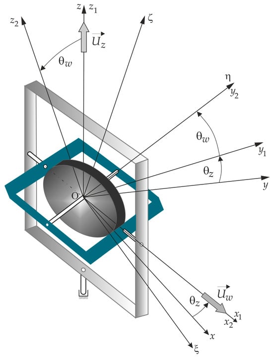
Figure 1.
Diagram of the gyroscope.
The equations of motion for a controlled gyroscope system, mounted on a movable base, were derived using Lagrange equations of the second kind. The most general form of these equations is presented in [8,10]. For further consideration, we assume that the base is stationary, the rotor’s center of mass coincides with the center of rotation, and we neglect the inertia of the frames.
Then the mathematical model of the movement of the gyroscope is as follows:
After linearizing the above equations, we have:
where
—the tilt and deviation angles of the gyroscope axis in space;
—the longitudinal and transverse moments of inertia of the gyroscope rotor, respectively;
—gyroscope’s own rotation speed;
—the friction coefficients in the suspension bearings;
—the control moments.
The functional diagram of the control of a gyroscope is shown in Figure 2.
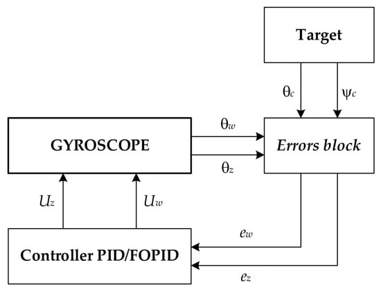
Figure 2.
The functional diagram of gyroscope control.
The task of the gyroscope is to track a detected moving target. The angles determine the position of the target, while the angles determine the actual position of the gyroscope axis. The target position angles are set signals in the gyroscope control system. In the Errors block, control errors are determined as the differences between the setpoint signal, i.e., angles , and the actual signal, i.e., angles . The determined control errors are sent to the PID/FOPID controller, which generates control signals applied to the gyroscope frames.
2.2. Controllers
For the gyroscope control process, two controllers were designed:
- the classical proportional–integral–derivative (PID) controller;
- the fractional-order proportional–integral–derivative (FOPID) controller.
PID controllers are very popular due to their structural simplicity and good performance, including a low percentage overshoot and a short settling time for slow processes [14].
In turn, the fractional-order PID controller demonstrates superior effectiveness compared with the classical PID controller, especially in the case of strongly nonlinear systems. Its main advantages are [14]:
- for higher-order systems it ensures better performance;
- it can easily achieve the iso-damping property;
- it is more robust and stable;
- it can control systems with nonlinearities more effectively.
- Classical PID controller
The control law for the classical PID controller is expressed as:
where
—the control errors given by: , ;
—the angles defining the target position in space;
The coefficients of the PID controller and were selected optimally using the fmincon function in the MATLAB environment [23]. The fmincon function is used to find the minimum of a given function (in this case, the costfun function) taking into account constraints. The following syntax of this function was used:
where
costfun—cost function to minimize.
x0—starting vector for optimization.
[] [] [] []—no linear constraints A, b, Aeq, beq.
lb, ub—lower and upper limits for the components of vector x.
[]—no nonlinear constraints (nonlcon).
options—optimization algorithm options (method, tolerances, iteration limits).
The structure of the PID controller is shown in Figure 3.
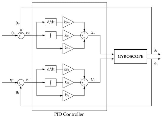
Figure 3.
The structure of the classical PID controller.
- Fractional-Order PID Controller [24]
The FOPID (Fractional-Order PID) controller is an extension of the classical PID controller, in which integration and differentiation are performed in fractional orders. By introducing the additional parameters of the integration order (λ) and the differentiation order (μ), it becomes possible to adjust the dynamic characteristics of the system more precisely. This type of controller makes it possible to achieve higher control quality and greater disturbance rejection compared with the classical PID, particularly in systems with complex or nonlinear dynamics.
where
—order integration ;
—order differentiation .
The structure shown in Figure 4 illustrates the implementation of the fractional-order PID controller (FOPID) in the control system of the two angular components and of the gyroscope axis position. The system consists (similarly to the classical controller presented above) of two independent control loops—the upper one for the variable and the lower one for the variable . At the input of each loop there is a summing junction that determines the control error identically as in the PID controller.
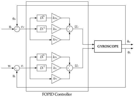
Figure 4.
The structure of the FOPID controller.
The error signal is then directed in parallel to three branches corresponding to the fractional-order differentiating element , the fractional-order integrating element and the proportional element.
- The differentiating branch implements the operator , followed by the gain .
- The integrating branch implements the operator , followed by the gain .
- The proportional branch implements only the gain .
The signals from the three branches are summed in the summing junction, forming the control signals and , respectively. These signals are then applied to the controlled object—the gyroscope system—which generates the outputs and . The output values are fed back to the input summators, thus closing the feedback loops.
According to the definition, fractional calculus constitutes a generalization of integration and differentiation operations to the case of an operator of non-integer order , where a and t denote the limits of the operator’s action, and α specifies the fractional order of this operation.
where it is usually assumed that , although it may also be a complex number.
In fractional-order operator calculus, there are several theoretically equivalent definitions of derivatives and integrals, including those of Riemann–Liouville, Caputo, and Grünwald–Letnikov [16,17].
The Grünwald–Letnikov definition is a direct discrete counterpart of the fractional-order differential definition, in which the operator is expressed as a finite weighted sum of the signal values from the current and past sampling instants:
where denotes the integer part of the argument, and is the generalized Newton coefficient. A discrete form of this operator, more convenient for numerical calculations, is often used in the form:
where the coefficients can be determined recursively:
This approach is particularly advantageous in numerical implementations of FOPID controllers, as it enables:
- Easy implementation—the coefficients are determined by a simple recursion, and the computations at each step reduce to multiplications and additions.
- Natural inclusion of signal memory—the operator requires only the storage of a buffer of finite length, which makes it possible to regulate the trade-off between accuracy and computational complexity.
- Universality—the same algorithm can be used both for integrals (), and derivatives (), and it also easily yields the classical case ().
- Easy transition from FOPID to PID—for and the operator reduces to the standard rectangular derivative and integral, which enables a full comparison of PID and FOPID within the same computer algorithm.
For these reasons, in the presented FOPID controller algorithm, the implementation in the Grünwald–Letnikov (GL) form was chosen, although alternative definitions (e.g., Caputo) are also mathematically correct. The key factors here were: ensuring minimal computational effort in simulations with a very small time step (), easy integration with the PID code without changing the structure of the computational loop, and the possibility of accurately reproducing the classical PID by setting the parameters .
The introduction of fractional-order integration and differentiation operators enables more precise shaping of system dynamics than in the case of the classical PID, allowing for better tuning of the transient response and damping properties over a wide frequency range. As a result, the FOPID controller is characterized by greater flexibility in adapting to systems with complex dynamics.
2.3. Control Performance
The assessment of control quality in a closed-loop system can be carried out using typical performance indices, e.g., settling time, steady-state error, Integral of Absolute Error, Integral of Squared Error, Integral of the Time-weighted Squared Error, Integral of Control.
The following quality indices were adopted:
- Quality index IAE (Integral of Absolute Error):
- Quality index ISC (Integral of Control):
An additional index:
- The mechanical energy described by Equation (13), i.e., the total work performed by the control moments in both gyroscope axes during the simulation time,
These indices enable a quantitative evaluation of the effectiveness of the control system under various dynamic conditions. The IAE is particularly useful in the analysis of systems where minimizing deviations from the reference value over the entire duration of the process is of crucial importance. The value of this index increases with the length of the error duration interval as well as with the error amplitude, which allows for a quick comparison of the control quality achieved by different control algorithms.
In turn, the ISC index reflects the level of the control signal energy delivered to the plant, which is important from the standpoint of energy efficiency and hardware limitations. Low ISC values indicate smoother controller action and reduced load on the actuators, which can contribute to extending their service life. Considering both indices simultaneously allows for a comprehensive evaluation of both the control accuracy and the cost of its implementation in terms of control energy consumption. This approach is particularly important in mechatronic systems, where high control precision must be reconciled with the power and speed limitations of the components.
3. Simulation Studies
In order to evaluate the performance of the designed PID and FOPID controllers, a series of simulation studies was conducted on the dynamics of the controlled gyroscope, described by Equations (3), for four scenarios.
Each scenario is based on the mathematical model of the plant, i.e., two equations of motion with strong gyroscopic couplings and viscous damping , integrated using the fourth-order Runge–Kutta (RK4) method, with the parameters: , , , . In the same formulation, feed-forward terms also appear: , , where the cross-axis couplings are several tens of times larger than the local damping and dominate the system dynamics.
The simulations were carried out in the Matlab/Simulink environment, using the ode4 integration procedure, with a fixed integration step of .
3.1. Simulation Results
- Scenario 1
In this scenario, the target’s set position angles (forming reference trajectory) change according to , , where , , corresponding to constant acceleration in the -channel and constant velocity in the -channel. Differentiating, we obtain: , and , , which directly enter the feed-forward compensation terms , . In practice, this means increasing moment demand in the and a constant moment in the , where in the the dominant component is , and in the —it is . Due to the coupling term— the growing acts like a “counter-torque” in the , which requires appropriately larger to maintain a small tracking error. From the stability perspective, the smooth spectrum of the reference signal does not excite high-frequency modes, which reduces sensitivity to the implementation of fractional operators. It is worth emphasizing implementation consistency: the plant loop exactly realizes the above equations with couplings and viscous damping, while the references are generated directly from the given formulas.
For a specified target angular velocity—, the tuning frequency , was applied, due to the slow tracking of the monotonic trend of trajectory changes without excessive differentiation of the object motion. The frequency was determined separately in each scenario so that the control loop bandwidth was matched to the bandwidth of the reference signals and the maneuver dynamics.
The figures below present the obtained time histories of the tilt () and deviation () angles of the gyroscope axis for the fractional-order PID (FOPID) controller.
In Figure 5a it can be observed that the response coincides with the reference trajectory over the entire horizon, without overshoot or delay. In the tilt channel, the curvature increases with time (increasing acceleration), yet no degradation of tracking accuracy is visible. In the deviation channel, the growth is linear and consistent, which indicates a well-tuned proportional–derivative component in both controllers. The residual error (Figure 5b) remains at the level of about 10−3 rad and is constant. It can be concluded that, in this configuration, the system correctly compensates cross-axis couplings and damping, ensuring accurate reproduction of the trajectory in both axes.
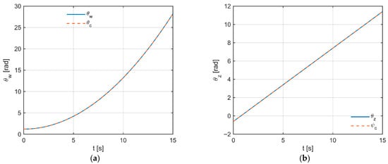
Figure 5.
Trajectories of tilt and deviation angles: (a) and ; (b) and . Solid line—response, dashed line—reference trajectory.
In Figure 6a, the control moments do not reach their limiting values: in the tilt channel they are nearly constant (~25 Nm) with minor correction, while in the deviation channel they decrease linearly to about −160 Nm, reflecting coupling compensation. The tilt error (Figure 6b) decreases linearly to about −1.2 × 10⁻³ rad, while the deviation error remains at about −0.2 × 10⁻³ rad. The absence of oscillations and saturation indicates stable gain tuning and effective feed-forward action.
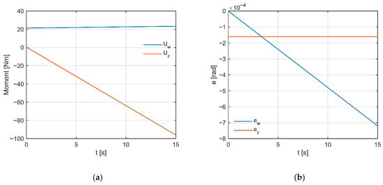
Figure 6.
(a) Control moment in the tilt and deviation channels. (b) Angular error in both channels.
The trajectory in the angle plane of the system (Figure 7a) almost perfectly coincides with the reference path; the absence of loops and deviations indicates negligible delay and effective coupling compensation. The trajectory is monotonic and smooth, confirming stable operation of the controllers (PID/FOPID) throughout the entire range of motion. In Figure 7b, the cumulative IAE error increases smoothly, which is the result of a constant, very small tracking error. The absence of breaks in the IAE curve indicates that neither saturation nor oscillations occur.
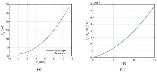
Figure 7.
(a) Path in the angle plane: system (Gyroscope) vs. reference (Reference). (b) Cumulative error over time (IAE).
- Scenario 2
In Scenario 2, the reference trajectory describes a smooth, low-frequency oscillation of tilt and a slow drift of the target deviation: and . The derivatives are: and , while , . Thus, the feed-forward terms periodically compensate inertia and damping , while in the dominant component is (constant). Due to the gyroscopic coupling , the instantaneous maximum of translates into an additional term in the -channel, which forces symmetric tuning of both loops. The profile is “light”: , , , hence very low frequencies dominate and the controller can operate with a small gain D without the risk of noise amplification. From a qualitative perspective, the IAE is a good measure of the “smoothness” of sinusoidal tracking—the integral of the error magnitude increases mainly at tunings that lag the phase relative to . From the plant dynamics perspective, this scenario verifies the ability to track quasi-stationary motion of the control signal (ISC). This results from the fact that derivative and fractional terms are not strongly excited. For this reason, in the simulation program the chosen tuning frequencies were somewhat higher than in Scenario 1 (here ), to minimize phase lag while maintaining moderate control energy.
In Figure 8a, in the tilt channel the response faithfully reproduces the sinusoidal trajectory: the extrema occur at the same instants of time, with no visible delay or waveform distortion. In Figure 8b, in the deviation channel the response to the linear ramp coincides with the reference point by point; the observed error has the form of a constant, very small bias (on the order of 10−3 rad). In both cases the signals are smooth, with no signs of saturation or oscillations, which indicates properly selected gains and effective compensation of cross-axis couplings.
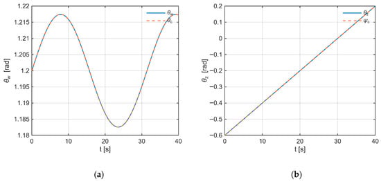
Figure 8.
Trajectories of tilt and deviation angles: (a) and ; (b) and . Solid line—response, dashed line—reference trajectory.
The control moment (Figure 9a) remains nearly constant (~0.53 Nm) with a slight drift, while varies smoothly in a sinusoidal manner within about ±0.1 Nm; both signals are smooth and show no signs of saturation. Figure 9b shows the errors: oscillates symmetrically around zero at the level of single microradians (≈±1 µrad), and has a constant, small steady-state value of about −4 µrad. The absence of a growing trend and the lack of oscillations indicate stable operation and correct compensation of cross-axis couplings.
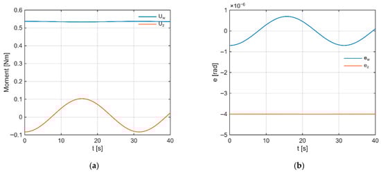
Figure 9.
(a) Control moment in the tilt and deviation channels. (b) Angular error in both channels.
Analyzing Figure 10a, it can be stated that the “Gyroscope” and “Reference” curves overlap almost perfectly; the absence of loops in the parametric plot indicates negligible phase delay and no hysteresis. The trajectory of the angles is smooth, and the transitions through extrema do not introduce noticeable deviations. In Figure 10b, the cumulative IAE error increases almost linearly to about 1.8 × 10⁻⁴, which indicates a constant, microradian-level error without episodes of abrupt changes. A slight change in slope halfway through the plot correlates with the change in trajectory curvature (Figure 10a), but does not affect stability.
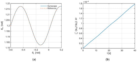
Figure 10.
(a) Path in the angle plane: system (Gyroscope) vs. reference (Reference). (b) Cumulative error over time (IAE).
- Scenario 3
In the third scenario, describing a spiral descent, the commanded motion is defined by the following relations: , with , and drift . The corresponding derivatives are: , , , . Thus, the feed-forward term compensates the periodic inertia and the coupling with , while —compensates the periodic inertia and the coupling with .
The adopted parameter values are: , , , , . These values cause the -channel to be about three times “faster” than the -channel, which reduces the influence of the coupling term—since faster oscillations of generate larger disturbances in the -equation. This requires more aggressive tuning () and a stronger role of the branch D (or fractional ) in order to reduce phase error. From the standpoint of indicators, IAE increases primarily due to phase mismatches, while ISC reflects the cost of changing the coupling direction at two distinct frequencies. This profile is also a good robustness test against saturation, since the component can momentarily amplify and thus the required compensating moment.
Figure 11a presents the tilt angle, where the response coincides with the trajectory composed of two periodic components, and the effect of the linear component is visible as a slow drift.
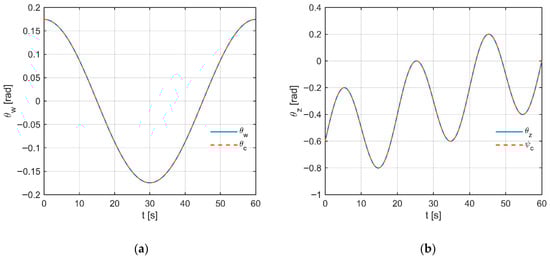
Figure 11.
Trajectories of tilt and deviation angles: (a) and ; (b) and . Solid line—response, dashed line—reference trajectory.
For the deviation (Figure 11b), a clearly varying amplitude can be observed, which confirms the superposition of two frequencies, while the mean value changes in accordance with the linear term. Both curves remain smooth and free from overshoot. Such a set of components generates, in the plane, a spiral-shaped trajectory.
The dominant control amplitude occurs in the tilt channel (Figure 12a) (≈±3 Nm, quasi-sinusoidal), while in the deviation channel the range is clearly smaller (≈±0.5 Nm) and slowly modulated. In Figure 12b, the tilt error oscillates around zero with an amplitude on the order of 10−5 rad, whereas in the deviation channel it has a larger amplitude. No saturation or fast oscillations are observed; the frequency content of the errors corresponds to the excitation (two periodic components plus a linear component—linear trend). Thus, it can be concluded that the system maintains tracking accuracy at the microradian level with moderate values of control moments.
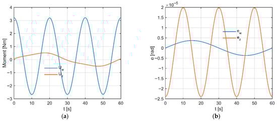
Figure 12.
(a) Control moment in the tilt and deviation channels. (b) Angular error in both channels.
The trajectory in the plane (Figure 13a) forms a series of closed loops of varying size—a typical beating effect resulting from the superposition of two periodic components. The “Gyroscope” and “Reference” curves practically coincide, which indicates negligible delay and no hysteresis. In Figure 13b, a monotonic increase of the IAE with superimposed modulation of the beating period (frequency difference) can be observed. The slope is nearly constant, and local variations correspond to phases of larger motion amplitude. The absence of breaks confirms the lack of saturation and forced oscillations.
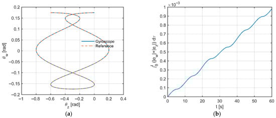
Figure 13.
(a) Path in the angle plane: system (Gyroscope) vs. reference (Reference). (b) Cumulative error over time (IAE).
- Scenario 4
The fourth scenario presents an obstacle-avoidance maneuver using a reference for the deviation angle, constructed from two minimum-jerk segments separated by a pause:
, where and , , .
In the implementation: , , , . The function has zero first and second derivatives at the endpoints, which ensures a smooth start and stop without jumps in reference velocity or acceleration. From these definitions, the derivatives used in the compensation follow: with and and and, in the simulation algorithm, and .
For the tilt angle, a proportional term with respect to the deviation rate is generated: , in the simulation algorithm. To avoid discontinuities under tilt limitation, a smooth saturator is applied: with . This choice guarantees —class continuity of the reference itself and allows one to compute its derivatives without jumps: and the second derivative over time , obtained via the chain rule (in the algorithm, the relations and the derivative of were used). Thanks to this, even when reaches the limiting zone, both and , remain smooth.
Thus defined, enter the feed-forward terms according to the coupled-axis model: in the channel, inertia and damping are compensated together with the gyroscopic coupling from term ; in the channel, analogous compensation is applied . The pause between the acceleration and deceleration phases prevents overlapping of the segments and maintains maneuver symmetry. The adopted values , limit the maximum control demands, while—thanks to the complete derivatives—the feed-forward takes over the majority of the dynamics. This reduces IAE and the moment peaks compared to a hard limiter. The entire formulation remains fully consistent with the coupled-axis model structure used in the previous scenarios.
Figure 14a shows the tilt induced by gyroscopic coupling. Two short-lived deflections of opposite signs occur here, strictly synchronized with the instants of jerk changes (Figure 14b), after which the signal returns to zero. In both channels, there are no overshoots or oscillations, which indicates properly tuned gains and effective coupling compensation.
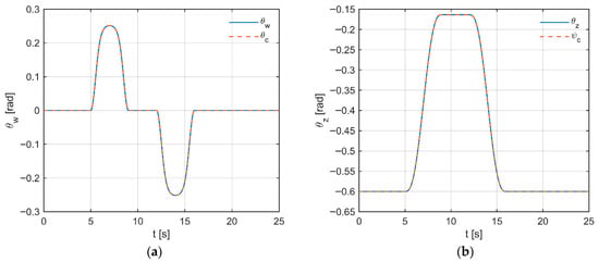
Figure 14.
Trajectories of tilt and deviation angles: (a) and ; (b) and . Solid line—response, dashed line—reference trajectory.
In Figure 14b, the response in the deviation axis faithfully reproduces the minimum-jerk reference profile: the rise and fall are smooth (C2 continuity), the steady segment is stable, and the error remains negligible and trend-free. It can therefore be concluded that the maneuver with jerk-limited reference is executed stably and with high accuracy in both axes.
In Figure 15a, short, smooth moment pulses are shown, synchronized with the beginning and end of the minimum-jerk segments in the deviation axis. The amplitude in deviation is larger (≈±8 Nm), while in the tilt channel compensating pulses appear (≈±6 Nm), resulting from gyroscopic couplings. The waveform shape (without sharp corners) is consistent with jerk limitation and indicates the absence of saturation.
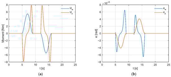
Figure 15.
(a) Control moment in the tilt and deviation channels. (b) Angular error in both channels.
Analyzing Figure 15b, one can observe transient error variations on the order of 10−5 rad, concentrated around the switching instants, which quickly decay to zero and show no significant trend. The absence of oscillations confirms proper damping and the effectiveness of the feed-forward term in compensating the couplings.
The parametric trajectory (Figure 16a) practically coincides with the reference trajectory, and the differences are below the resolution of the plot. The outline has a quasi-rectangular shape with smooth corners, consistent with the minimum-jerk profile with a constant segment. The absence of hysteresis indicates negligible phase lag. The IAE (Figure 16b) is piecewise linear, with steep increases occurring only in two transient phases, while in the constant segment the derivative of IAE ≈ 0. No peaks or ripples are present, suggesting operation without saturation and with proper damping.
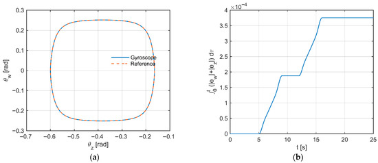
Figure 16.
(a) Path in the angle plane: system (Gyroscope) vs. reference (Reference). (b) Cumulative error over time (IAE).
In all four scenarios, the reference trajectories () are explicitly differentiable (except for the saturation points in the S-curve), which makes it possible to directly build feed-forward compensation based on the first and second derivatives over time, as well as the model parameters. In each scenario, the dominant challenge is the cross-coupling term , which, for the parameters used, exceeds the local viscous damping by several tens of times (≈54×), shaping the system dynamics. Therefore, the or branch has a real impact on reducing phase error. The performance indices are consistent: , —where IAE evaluates tracking accuracy and ISC measures control cost. In Scenarios 1–3, IAE increases mainly due to phase delays, and in Scenario 4 additionally due to saturation. The main modeling challenges result from selecting and controller parameters so as to handle references with different bandwidths and strong couplings, while ensuring proper implementation of fractional operators (Oustaloup + Tustin with pre-warping to or discrete Grünwald–Letnikov with memory horizon ), which requires attention to reproducing both modulus and phase, as well as saturation handling and anti-windup in Scenario 4. From a mathematical standpoint, all scenarios can be expressed in a unified state-space form: with , and reference given as (). In the quality loop we analyze , together with IAE and ISC as defined above.
3.2. Comparative Analysis of PID vs. FOPID
In this subsection, a comparative analysis of two types of control—PID and FOPID—is presented, based on the simulation results. The parameters resulting from the tuning of the controllers are summarized in Table 1, while the control performance indices and their values are given in Table 2.

Table 1.
Controller gains.
Table 2.
Tracking and control performance indices.
For Scenarios 1–3, the indices of the integral control cost and mechanical energy were practically indistinguishable between PID and FOPID (e.g., Sc.2: IAE = 0, ISC = 11.632 Nm2·s, Emech = 8.119 × 10⁻³ J; Sc.3: IAE ≈ 10−6, ISC = 269.916 Nm2·s, Emech = 0.188 J), and the RMS (Root Mean Square) values and peaks of the control moments coincided within the resolution limits of the data recording.
This implies that the main “carrier” of the control energy is the feed-forward component resulting from the plant model, while the feedback—regardless of the use of fractional-order integration and differentiation—only suppresses small residual tracking errors. This behavior is consistent with the RK4 implementation and derivative filtering (PID: Tf = 1; FOPID: discrete GL), which limit high-frequency gain and “equalize” the energy expenditure between the strategies.
A significant difference appeared only in the S-curve (minimum-jerk) profile, which generates a more demanding error spectrum in the mid-frequency range. In this case, FOPID achieved ~32.6% lower IAE (3.1 × 10⁻⁵ vs. 4.6 × 10⁻⁵) with practically identical control cost (ISC: 248.0538 vs. 248.057 Nm2·s; Δ ≈ 0.0013%) and mechanical energy (0.172671 vs. 0.172673 J). We associate the improvement in tracking quality with the additional degrees of freedom in FOPID—the orders λ, μ—which make it possible to achieve a “distributed” shaping of the phase shift in the frequency band where the minimum-jerk profile imposes the greatest demands.
The optima obtained in this scenario (for example: , and , ) confirm that a slight departure from order 1 makes it possible to reduce IAE without increasing energy expenditure and without raising the RMS/peaks of the control moments—which is desirable in applications with actuator limitations. It should be emphasized that the PID controller, under the same derivative filter configuration () and identical feed-forward, approaches the FOPID optimum in terms of ISC and Emech, but does not achieve the same IAE reduction. This indicates a “phase advantage” resulting from fractional-order differentiation.
For completeness: in Scenario 1, the differences between the controllers are within recording precision (e.g., ISC = 53 299.8437 Nm2·s and Emech = 37.351 J for both), which further supports the thesis of the dominant role of feed-forward in smooth trajectories. Similarly, in Scenarios 2 and 3, we obtain practically perfect convergence of PID and FOPID both in IAE and in RMS/peaks of the control signals.
4. Summary
A comparative analysis of the classical PID and the FOPID controllers for a 3-DOF gyroscope with gyroscopic couplings, using a complete model solved with the RK4 method and discrete GL/Oustaloup operators, confirmed comparable stability and performance of both control strategies. In scenarios with smooth references (ramp, low-frequency sinusoid, spiral descent), the IAE, ISC, and mechanical energy metrics proved to be practically indistinguishable, which indicates that the control cost was dominated by the feed-forward term derived from the plant model and compensating for inertia, damping, and cross-axis couplings.
The difference in quality became evident in the minimum-jerk profile: FOPID reduced IAE by ~33% compared with PID, with practically identical ISC and Emech, which we attribute to better phase-shift shaping in the excitation band of this maneuver. Additional degrees of freedom in FOPID (integration order λ and differentiation order μ) enabled fine-tuning of the characteristics without increasing RMS or peak moments, as confirmed by the values selected in this study, .
Under strong couplings both strategies maintained small errors thanks to explicit feed-forward compensation, derivative filtering, and anti-windup in the feedback loop. From an implementation perspective, the FOPID in the Grünwald–Letnikov form is computationally lightweight (finite-length buffer) and reduces to the classical PID for , which simplifies joint tuning and comparison.
In summary, for smooth trajectories and properly designed feed-forward, the classical PID is sufficient, whereas in tasks with constrained jerk or stricter requirements in the mid-frequency band, the FOPID provides a tangible improvement in tracking accuracy without additionally burdening the control actuators, which justifies further experimental validation and robustness testing.
Author Contributions
Conceptualization, I.K.; methodology, I.K. and S.B.; software, I.K. and S.B.; validation, I.K. and S.B.; formal analysis, I.K. and S.B.; investigation, I.K. and S.B.; resources, I.K. and S.B.; data curation, I.K.; writing—original draft preparation, I.K. and S.B.; writing—review and editing, I.K. and S.B.; visualization, I.K. and S.B.; supervision, I.K. and S.B. All authors have read and agreed to the published version of the manuscript.
Funding
This research received no external funding.
Data Availability Statement
No data was used for the research described in the article.
Conflicts of Interest
The authors declare no conflicts of interest.
References
- Scarborough, J.B. The Gyroscope Theory And Applications; Creative Media Partners, LLC: Sacramento, CA, USA, 2022; ISBN 9781015443938. [Google Scholar]
- Ge, Z.-M.; Lee, J.-K. Chaos synchronization and parameter identification for gyroscope system. Appl. Math. Comput. 2005, 163, 667–682. [Google Scholar] [CrossRef]
- Lei, Y.; Xu, W.; Zheng, H. Synchronization of two chaotic nonlinear gyros using active control. Phys. Lett. A 2005, 343, 153–158. [Google Scholar] [CrossRef]
- Sargolzaei, M.; Yaghoobi, M.; Yazdi, R.A.G. Modeling and synchronization of chaotic gyroscopes using TS fuzzy approach. Adv. Electron. Electr. Eng. 2013, 3, 339–346. [Google Scholar]
- Yau, H.-T. Generalized projective chaos synchronization of gyroscope systems subjected to dead-zone nonlinear inputs. Phys. Lett. A 2008, 372, 2380–2385. [Google Scholar] [CrossRef]
- Yau, H.-T. Chaos synchronization of two uncertain chaotic nonlinear gyros using fuzzy sliding mode control. Mech. Syst. Signal Process. 2008, 22, 408–418. [Google Scholar] [CrossRef]
- Roopaei, M.; Zolghadri Jahromi, M.; John, R.; Lin, T.-C. Unknown nonlinear chaotic gyros synchronization using adaptive fuzzy sliding mode control with unknown dead-zone input. Commun. Nonlinear Sci. Numer. Simul. 2010, 15, 2536–2545. [Google Scholar] [CrossRef]
- Awrejcewicz, J.; Koruba, Z. Classical Mechanics; Springer: New York, NY, USA, 2012; ISBN 978-1-4614-3977-6. [Google Scholar]
- He, H.; Xie, X.; Wang, W. Vibration Control of Tower Structure with Multiple Cardan Gyroscopes. Shock Vib. 2017, 2017, 3548360. [Google Scholar] [CrossRef]
- Krzysztofik, I.; Takosoglu, J.; Koruba, Z. Selected methods of control of the scanning and tracking gyroscope system mounted on a combat vehicle. Annu. Rev. Control 2017, 44, 173–182. [Google Scholar] [CrossRef]
- Lungu, M. Control of double gimbal control moment gyro systems using the backstepping control method and a nonlinear disturbance observer. Acta Astronaut. 2021, 180, 639–649. [Google Scholar] [CrossRef]
- Kojima, H.; Nakamura, R.; Keshtkar, S. Model predictive steering control law for double gimbal scissored-pair control moment gyros. Acta Astronaut. 2021, 183, 273–285. [Google Scholar] [CrossRef]
- Papakonstantinou, C.; Lappas, V.; Kostopoulos, V. A Gimballed Control Moment Gyroscope Cluster Design for Spacecraft Attitude Control. Aerospace 2021, 8, 273. [Google Scholar] [CrossRef]
- Shah, P.; Agashe, S. Review of fractional PID controller. Mechatronics 2016, 38, 29–41. [Google Scholar] [CrossRef]
- Edet, E.; Katebi, R. On Fractional-Order PID Controllers. IFAC-PapersOnLine 2018, 51, 739–744. [Google Scholar] [CrossRef]
- Podlubny, I. Fractional-Order Systems and Fractional-Order Controllers; Institute of Experimental Physics Slovak Academy of Sciences: Kosice, Slovakia, 1994. [Google Scholar]
- Monje, C.A.; Chen, Y.; Vinagre, B.M.; Xue, D.; Feliu-Batlle, V. Fractional-Order Systems and Controls: Fundamentals and Applications; Springer Science & Business Media: Berlin/Heidelberg, Germany, 2010. [Google Scholar]
- Valerio, D.; Costa, J. Tuning rules for fractional PID controllers. In Proceedings of the 2nd IFAC Workshop on Fractional Differentiation and Its Applications, Porto, Portugal, 19–21 July 2006; pp. 1–6. [Google Scholar]
- Padula, S.; Visioli, A. Tuning rules for optimal PID and fractional-order PID controllers. J. Process Control 2011, 21, 69–81. [Google Scholar] [CrossRef]
- Oprzędkiewicz, K.; Podsiadło, M. The Fractional Order PID Control of the Forced Air Heating System. Pomiary Autom. Robot. 2019, 1, 5–10. [Google Scholar] [CrossRef]
- Petras, I. Fractional—Order feedback control of a DC motor. J. Electr. Eng. 2009, 60, 117–128. [Google Scholar]
- Krzysztofik, I.; Blasiak, S. Analytical Solutions of the 3-DOF Gyroscope Model. Electronics 2024, 13, 1843. [Google Scholar] [CrossRef]
- Tewari, A. Modern Control Design with MATLAB and Simulink; John Wiley & Sons: Hoboken, NJ, USA, 2002. [Google Scholar]
- Tepljakov, A.; Petlenkov, E.; Belikov, J.; Finajev, J. Fractional-order controller de- sign and digital implementation using fomcon toolbox for MATLAB. In Proceedings of the 2013 IEEE Conference on Computer Aided Control System Design (CACSD), Hyderabad, India, 28–30 August 2013; pp. 340–345. [Google Scholar] [CrossRef]
Disclaimer/Publisher’s Note: The statements, opinions and data contained in all publications are solely those of the individual author(s) and contributor(s) and not of MDPI and/or the editor(s). MDPI and/or the editor(s) disclaim responsibility for any injury to people or property resulting from any ideas, methods, instructions or products referred to in the content. |
© 2025 by the authors. Licensee MDPI, Basel, Switzerland. This article is an open access article distributed under the terms and conditions of the Creative Commons Attribution (CC BY) license (https://creativecommons.org/licenses/by/4.0/).