Article

Graph-DEM: A Graph Neural Network Model for Proxy and Acceleration Discrete Element Method

1
SKLSDE and BDBC Lab, Beihang University, Beijing 100191, China
2
School of Transportation Science and Engineering, Beihang University, Beijing 100191, China
3
Faculty of Architecture, Civil and Transportation Engineering, Beijing University of Technology, Beijing 100124, China
*
Authors to whom correspondence should be addressed.
Appl. Sci. 2025, 15(19), 10432; https://doi.org/10.3390/app151910432
Submission received: 9 September 2025 / Revised: 19 September 2025 / Accepted: 21 September 2025 / Published: 26 September 2025

Abstract

The discrete element method (DEM) is widely employed in various fields for analyzing rock and soil movement. However, the traditional DEM involves a large number of calculations, which leads to reduced computational efficiency. Deep-learning presents a promising solution to this issue by utilizing neural networks to approximate DEM calculations. Moreover, the consistency between the arrangement of discrete particles and the structure presented in graph neural networks further reinforces the validity of this approach. In this study, we propose a novel model called Graph-DEM based on graph neural networks, which significantly enhances the speed of DEM calculations. Meanwhile, our model demonstrates the capability of adaptive learning across various constitutive relationships. To evaluate the model’s performance, we measure particle-trajectory prediction accuracy on three scenario datasets (dynamic, static, and principle experiments) and on two public datasets. In addition, the computational efficiency of the Graph-DEM model are compared against the traditional DEM. The experimental results demonstrate the superiority of the model in terms of accuracy, universality, and computational efficiency.

1. Introduction

Geotechnical materials appear to be relatively continuous at the macroscopic level, but at the microscopic level, they are composed of a structural system of particles, pores, and cracks. The discreteness and heterogeneity of geotechnical materials make it difficult to analyze them using conventional mechanics methods based on continuous media. The discrete element method (DEM) [1] is based on Newton’s laws of motion and calculates the interaction relationships between particles to analyze the force and motion trends of the particles, thus analyzing the changes in geotechnical structures. Due to its capacity to simulate the interaction of microscopic particles and consider discontinuous behavior, the DEM has been widely applied in various fields such as geology and geotechnics following years of development. Particularly in engineering scenarios involving materials such as sand and ballast, the DEM has emerged as an indispensable tool.
However, with the scaling and complexity of the models and the application requirements of specific scenarios, the low computational efficiency of the discrete element method have become a disadvantage. In recent years, with the advancement of hardware computational capabilities, Chun Liu at Nanjing University developed large-scale three-dimensional DEM software, namely, MatDEM v2.02 [2] (http://matdem.com/, accessed on 20 September 2025), for soil and rock mechanics. This software employs an innovative contact search algorithm and GPU matrix computation method, which greatly enhances its computational efficiency. Nevertheless, despite these improvements, the DEM still requires a considerable amount of time to solve large-scale and multi-physics coupled problems. The pursuit of advanced techniques to optimize computational efficiency is an extremely pressing matter.
Recently, deep learning methodologies have rapidly developed, giving rise to diverse approaches such as RNNs [3], CNNs [4], GNNs [5,6], and transformers [7], which have permeated our daily lives. With the advent of the data era, the use of deep learning methods to address challenges and limitations in various disciplines has become a trend, owing to their ability to extract potential patterns from massive quantities of data. In the field of geotechnical engineering, deep learning methods have been applied in landslide prediction [8], geotechnical reliability analysis [9], and intelligence-assisted driving of tunneling machines [10], to name but a few. Moreover, compared to traditional discrete element models, such as linear contact models [1], deep learning methods can simplify and compress the complex calculation process of particle displacement into a learnable parameter matrix, thereby enhancing computational efficiency.
Among these deep learning methods, RNNs are particularly well suited for processing sequential data such as natural language text, audio, and time-series data. CNNs are better suited for extracting features in a local region and are particularly useful for processing two-dimensional data such as images and videos. The transformer architecture utilizes self-attention mechanisms to capture dependencies between elements in a sequence and is particularly well suited for processing long sequential data. Compared to them, graph neural networks (GNNs) model the nodes and edges of a graph structure and learn from their interrelationships. GNNs are particularly advantageous in processing unstructured graph data such as social networks [11] and chemical molecular structures [12]. Due to the fact that the discrete element method abstracts soil or rock masses into unstructured particles, using GNN models to replace the discrete element method is undoubtedly the most natural and suitable choice.
We demonstrate the potential consistency between the discrete element method and GNNs through a set of figures. Figure 1a displays the distribution of particle positions. In order to calculate the displacement of particles, the linear-elasticity contact model represents interacting particles by computing the normal and tangential forces between particles. The normal force is calculated through a “repulsion–attraction” spring force and the tangential force is also obtained through breakable elastic springs along the tangential direction, as shown in Figure 1b. From a macroscopic perspective, the “particle–spring” topology bears a striking resemblance to the “node–edge” structure depicted in the diagram, as shown in Figure 1c. When considering the system from a microscopic perspective, the displacement of particles is influenced by the springs, and the interaction between particles is transmitted through the springs, aligning with the concept of graph neural networks that propagate node influence through edges.
Based on this potential similarity, we present a novel graph neural network model, Graph-DEM, which is inspired by discrete element computation methods. Graph-DEM leverages a graph structure to represent the geotechnical particle structure and learns the interaction relationships between particles by correlating and computing adjacent particles. This enables our model to accurately predict the displacement of particles. We evaluate Graph-DEM on three scenarios and demonstrate its consistency with the ground-truth values. Moreover, our model enhances the computational efficiency of geotechnical particle trajectory calculation by replacing complex numerical calculations with learnable neural network fitting. This enhancement in computational efficiency significantly increases the feasibility of applying discrete element-like computation methods in practical engineering applications.
In addition, since multi-layer neural networks containing activation functions can theoretically fit any functional relationship [13,14], substituting the physical numerical calculation with a learnable parameter matrix enables our model to adaptively learn various constitutive relationships, including linear elasticity, elastic plasticity, superelasticity, etc. Moreover, this approach not only can simulate contact relationships within two- or three-dimensional spaces but also obviates the need to select appropriate constitutive relationships and parameters for different computational instances.
This paper makes the following contributions:
  • We propose a graph neural network model, namely, Graph-DEM (The code and data can be found at https://github.com/LIPO714/Graph-DEM, accessed on 20 September 2025), which can predict the trajectories of geotechnical particles. It exploits the unique topological structure of graphs and learnable neural networks to approximate the physical computation in the discrete element method.
  • We construct three experimental datasets with different constitutive relations that reflect dynamic experiments, static experiments, and principle experiments, respectively. We validate the prediction performance of our model on these three datasets.
  • We demonstrate the model’s accuracy by evaluating both the overall motion trends of geotechnical structures and the particle-trajectory predictions on the three constructed datasets, and we further assess its competitiveness on two public benchmarks. Additionally, we demonstrate and discuss the universality of our proposed framework for different constitutive equations through accurate predictions in different cases.
  • We compare the computational efficiency of our model with conventional DEMs and show its advantage in this aspect.
The outline of this paper is as follows: Section 2 reviews the development status and research foundation of the discrete element method and graph neural network. Section 3 presents the necessary formal definitions, including the formalization of the studied problem, and the formalization of the graph. Section 4 introduces Graph-DEM’s structure and implementation in detail. Section 5 presents the experiments, including detailed information on our three datasets, the model input, training process, and evaluation process. The complete process of deep learning is explained in Section 5.4. Section 6 presents the evaluation results of the model and discusses the accuracy of predicted particle positions and the computational efficiency of the model.

2. Related Work

This section provides a brief overview of the development and current bottlenecks of discrete element methods (DEMs), as well as the advancement represented by graph neural networks (GNNs) and the feasibility of applying deep learning to physics simulations.

2.1. Discrete Element Method

In 1971, Cundall proposed the discrete element method (DEM) for rock mechanics, and in 1979, Cundall and Strack further extended the DEM to soil mechanics, establishing a more comprehensive soft-particle model and methodology [1]. The discrete element method boasts significant advantages in addressing issues such as particle permeability, stability of particle accumulation structures, and deformation properties [15], finding extensive applications in slope engineering, excavation engineering, and tunnel engineering.
The discrete element method seeks to investigate the macroscopic properties of particle systems by numerically simulating interparticle interactions. It decomposes the particulate matter system into separate discrete elements, where each element interacts with others via a simplified mechanical model. Contrary to the traditional finite element method, the discrete element method permits relative motion between units without necessarily adhering to displacement continuity and deformation coordination conditions. By integrating the discrete element method with other numerical approaches, multiscale [16] and multiphysical field [17,18] coupled simulation techniques have emerged, facilitating more precise modeling of complex particle system behavior.
Liu Chun from Nanjing University pioneered the development of the large-scale, three-dimensional geotechnical discrete element software MatDEM v2.02, employing cutting-edge contact search algorithms and GPU matrix computation methods to significantly enhance computational efficiency. This advancement enabled the first-ever dynamic simulation of millions of units and energy conservation simulation [2] on a single computer. The computational efficiency and unit count of MatDEM surpasses that of the commercial software PFC by a factor of 30. Nevertheless, the discrete element method still demands substantial time to tackle large-scale, multiphysical field coupling problems. In order to overcome these drawbacks, researchers are delving into multiscale and multiphysical field coupling computational methodologies [19], aiming to enhance the calculation speed of the discrete element method. Factors such as the model’s scale and complexity exert considerable influence on calculation speed, with particle contacts and collisions exerting an even greater impact. As a result, the exploration of these advanced methodologies is crucial for addressing the inherent challenges associated with the discrete element method, ultimately improving its efficiency and applicability in large-scale, complex problem-solving contexts.

2.2. Graph Neural Network

In recent years, with the rapid development of neural networks and deep learning, people have used various deep neural network structures to mine the potential rules in huge data and hidden useful information. In view of their low cost and high reliability, deep learning methods have gradually replaced manual methods in many fields, such as some classic networks like recurrent neural networks (RNNs) [3], convolutional neural networks (CNNs) [4], etc. Compared with their proven efficiency in capturing hidden patterns in Euclidean data, more and more applications show that graph structures are more suitable for representing non-Euclidean data. Therefore, making neural networks adapt to graph structures has become an intriguing research topic.
Unlike regular data (e.g., images), graphs can represent irregular data with their unique topological structure. A graph consists of a certain number of nodes, which are connected by some edges. Furthermore, complex graphs can carry richer information on nodes and edges. Graphs can be classified based on various criteria: directionality (directed or undirected), homogeneity (homogeneous or heterogeneous [20]), dynamics (dynamic [21] or static), and specific (hypergraphs). Generally, the graph structure design also affects the information contained in the graph, which may change according to the research problem.
Graphs can capture complex and dynamic relationships among data, but they pose challenges for traditional neural networks that rely on operations such as convolution. To address this, F. Scarselli et al. introduced graph neural networks (GNNs) [5,6] in 2008, which can learn from hidden information in graphs by propagating messages across nodes and edges. Later, Thomas N. Kipf and Max Welling proposed graph convolutional networks (GCNs) [11], which generalize convolution-like operations to graph structures. Inspired by self-attention [7] mechanisms, Petar Veličković et al. proposed graph attention networks (GATs) [22], which assign different weights to the messages from neighboring nodes based on their relevance. The applications of GNNs span across node-level [23], edge-level [24,25], and graph-level tasks. In recent years, GNNs and their variants [11,22,26] have been widely adopted and developed in various domains such as transportation [23,27,28], biochemical [25,29], knowledge graph [30], recommendation systems [31,32], etc.
Physical simulation [33] is a major research area in both physics and graphics. By leveraging deep learning techniques and computer graphics, computers can emulate some intricate and fascinating physical phenomena, such as fluid dynamics [34,35,36], bread tearing [37], towel wringing [38], surface tension [39], etc.
For physics-based particle trajectory simulation, prior studies have explored diverse modeling paradigms across fluids and solids: regression forests coupled with the Navier–Stokes equations for fluid particles [40]; dynamic particle-interaction graphs in DPI-NET for fluid and solid particles [41]; graph-convolutional operators over particle graphs [42]; and the general Graph Network-based Simulator (GNS) for multi-physics particle simulation, with constrained and hierarchical variants such as C-GNS and HGNS [43,44,45]. In parallel, the GNN literature has converged on two physics-informed directions: (i) models that inject conservation laws (e.g., LNN/LGNN), which, however, are of limited applicability in dissipative solid/DEM regimes [46,47]; and (ii) symmetry-preserving equivariant architectures (e.g., EGNN/GMN/ESTAG), which predominantly target microscopic systems [48,49,50]. For gravity-dominated macroscopic granular media, SGNN and Solid-GN preserve horizontal-flip symmetry by introducing a gravity-direction vector or a lightweight symmetric interaction encoding, respectively [51,52]. Despite these advances, practical deployment often imposes additional structural restrictions (such as fixed mapped-filter matrices and convolutional calculations) and enforces physical constraints (e.g., strict conservation laws) that do not faithfully reflect real-world granular dynamics, ultimately limiting flexibility, scalability, and accuracy for engineering-grade DEMs.
Motivated by these gaps, we propose Graph-DEM, a GNN-based proxy framework for discrete-element systems that maps particles to nodes and contacts to edges and learns interparticle interactions via message passing. Across multiple scenarios, Graph-DEM achieves substantial speed-ups while maintaining competitive accuracy, thereby providing a practical surrogate for physics-based granular simulation that better accommodates complex, real-world conditions.

3. Preliminaries

This section provides further evidence of the potential similarity and consistency between graph neural networks (GNNs) and discrete element methods (DEMs), demonstrating the rationality of employing GNNs to model the discrete element process. Subsequently, this section provides the necessary formal definitions, including the formalization of the studied problem and the graph.

3.1. Model Consistency

As introduced in Section 1, the discrete element method with a linear contact model shares similarities and consistencies with GNNs in terms of macroscopic structure, design details, and model concepts. These similarities form the basis for the correct and effective prediction of particle displacement by our model.
As shown in Figure 1, the structure of “particle–spring” and “node–edge” is identical. Furthermore, we elaborate on the conceptual consistency between the two approaches. Graph neural networks utilize edge to propagate node features and properties, enabling information exchange among particles. For every pair of nodes connected by an edge, interaction between the nodes typically relies on the information features of the two nodes, such as their types, as well as edge properties, such as edge weight. In the linear contact model, the displacement of particles is influenced by normal and tangential spring forces between the particles. The computation of these spring forces is also jointly affected by particle features, such as physical properties, and spring features, such as the distance between the particles. Both methods rely on computations based on nodes and edges.
Overall, the graph structure serves as a powerful tool for capturing and analyzing the complex relationships and interactions between discrete elements in a system, thereby enabling a deeper understanding of system behavior. Based on this similarity, we designed our model. However, before delving into the specifics of the model, it is imperative that we provide some necessary clarifications and definitions.

3.2. Problem Formalization

The information set corresponding to a physical system comprising N particles at timestamp t R + is denoted as X t = { x 1 t , , x i t , , x N t } . Naturally, we represent the historical information sequence of this system spanning the previous K time steps as X t K + 1 : t = X t K + 1 , , X t 1 , X t , where 1 K t .
In this context, x i t = { p i t , T i , f i } signifies the information vector pertaining to the ith particle at time t, encompassing the particle’s position p i t , particle type T i , and physical property parameters f i .
The simulation process frequently employs a multitude of particle physical property parameters to delineate the nature of particles. In our model, the particle type T i is utilized for a broad differentiation of the physical attribute disparities among particles. Moreover, for certain physical property parameters, the model facilitates direct input of these parameters f i to establish relationships between physical properties and the forces acting upon particles as well as their displacements. However, it is noteworthy that f i is discretionary.
In addition, we denote the velocity of the ith particle at time t as p ˙ i t and the acceleration as p ¨ i t . Their computation can be described by:
p ˙ i t = p i t p i t 1 p ¨ i t = p ˙ i t p ˙ i t 1 .
Based on the aforementioned definition, we can review and elucidate the computation process of the classical discrete element method (e.g., linear contact model) as follows:
P ^ t + 1 = D E M X t .
By providing the entirety of the current timestamp’s information, X t , the discrete element method (DEM) computes the positions of particles at the subsequent timestamp, denoted as P ^ t + 1 = p ^ 1 t + 1 , , p ^ i t + 1 , , p ^ N t + 1 . This iterative process is employed to simulate the trajectories of the particles.
Our goal is to learn the GraphDEM as follows:
P ¨ t + 1 = G r a p h D E M ( X t K + 1 : t ) ,
where we predict the acceleration of particles at the subsequent time step, P ¨ t + 1 , by employing the historical information sequence of the system, X t K + 1 : t , as input. Subsequently, based on Equation (1), we can compute the positions of all particles, P t + 1 .
In contrast to employing direct physical laws and formulas, as in the discrete element method, our model is constructed using a collection of trainable parameters. These parameters aim to conform to and approximate the underlying physical laws and formulas. To elaborate further, our model, due to its distinctive topological structure, has the capability to discern the influence exerted by neighboring particles on one another. It establishes a mapping relationship that connects the historical particle information and properties with future particle trajectories.
To extend the trajectory prediction beyond merely forecasting particle positions at a future time step, we proceed to construct the information for the t + 1 timestamp. At this juncture, we define x t + 1 = { p i t + 1 , T i , f i } and subsequently create a new historical information sequence denoted as X t K + 2 : t + 1 = X t K + 2 , , X t , X t + 1 . By employing Equation (3), we can then derive P t + 2 . This iterative process can be repeated, enabling us to predict the future trajectory of particles.

3.3. Directed Graph

Building upon the discussion in Section 3.1 regarding the importance of structural similarity, we adopt a graph-based framework to capture the historical information within the current discrete element system. In this context, we present a formal definition of the graph structure employed in this paper.
Consider a graph denoted G = ( V , E ) , comprising a node set V = v 1 , v 2 , , v N consisting of N nodes and an edge set E , where each v i V signifies a node within this graph. Furthermore, each node in V corresponds to a discrete particle within the system, while each edge in E signifies a physical connection existing between two adjacent elements. We propose to embed a “particle–spring” structure into a “node–edge” graph structure, where each particle is represented as a node and each spring as an edge, allowing for a unified representation of both the geometrical and topological information in the system.
In particular, in order to differentiate the interaction relationships between adjacent particles, we design the edges to be directional, thereby distinguishing the target nodes of these interactions. In practical terms, E R M × 2 with M edges consists of sender-node set S R M and receiver-node set R R M . Among them, e i j = ( v i , v j ) denotes a node pair, as well as the directed edge or interaction from node v i to node v j , where v i , v j V , e i j E , v i S and v j R . Generally, we call node v i the sender node of edge e m and node v j the receiver node. Additionally, since the interaction between particles is mutual, if e i j E , then an edge e j i = ( v j , v i ) will also in E .
To emphasize, the construction of edges in the graph is based on the distance between particles at the current time step, and the graph structure is updated at every time step to ensure real-time relationships between particles. Please refer to Section 4.2.2 for the specific process of constructing edges.

4. Graph-DEM

In this section, we dive into the elaboration of the proposed novel model structure. With the model structure presented below and the learnable parameter matrix, our model can fit the complex discrete element calculation process between particle pairs. Therefore, our model can grasp the particle motion law.

4.1. Overview

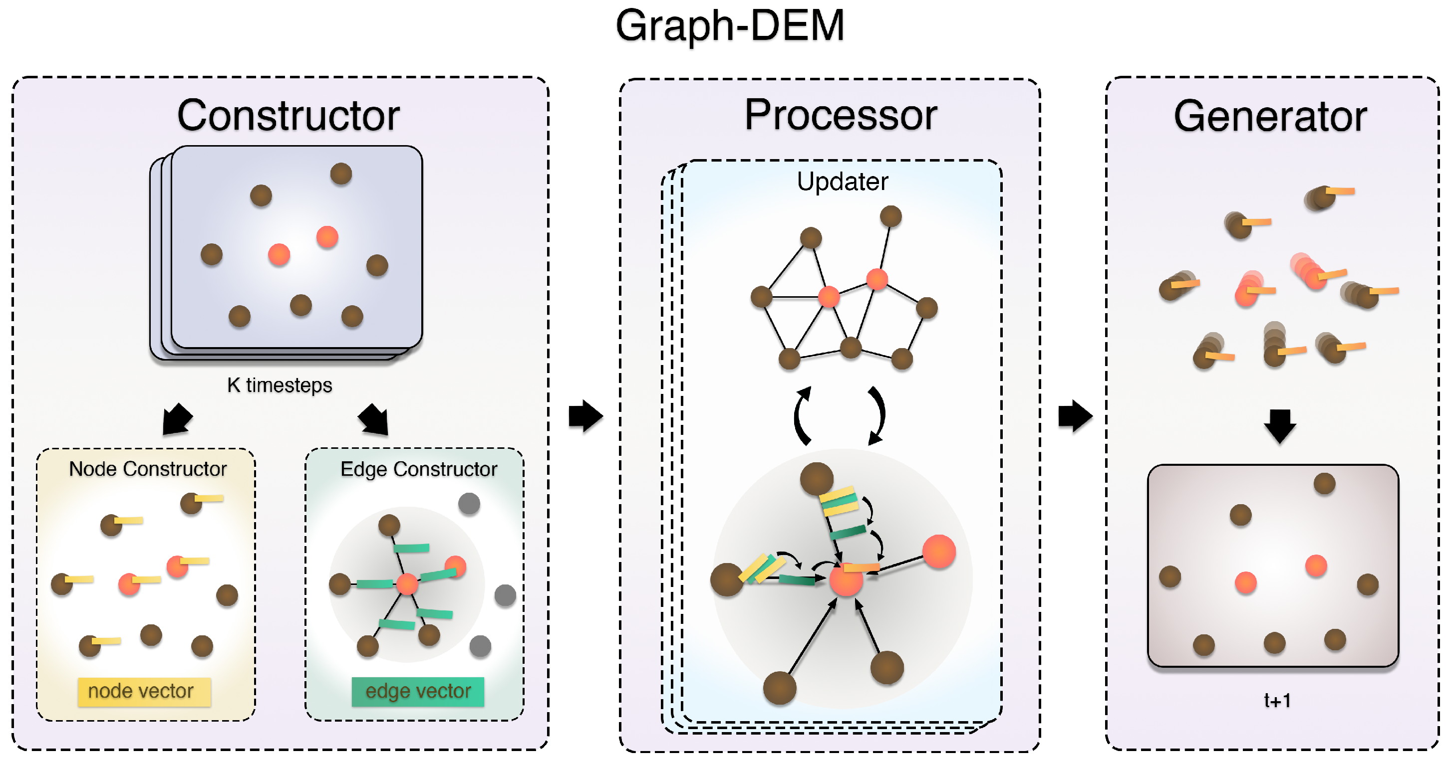
As presented in Figure 2, Graph-DEM mainly contains three core components.
Constructor. The constructor is responsible for mining and extracting the features in the system history information sequence X t K + 1 : t , transforming and embedding them into graph G 0 = ( V 0 , E 0 ) . More specifically, the constructor consists of a node constructor and an edge constructor, which are responsible for embedding information into the node feature vector set, V 0 , and edge feature vector set, E 0 , respectively. As shown in Figure 2, the node constructor puts yellow tags (node feature vectors) on each node, and the edge constructor puts green tags (edge feature vectors) on each edge. With the nodes embedded by particles and the edges constructed between nodes, discrete data are transformed into a tightly linked whole.
Processor. The role of the processor is to fit the physical law and the calculation process of discrete elements. It achieves this by simulating the influence of each neighboring particle on a given particle, using the edge connections as a basis. Subsequently, it consolidates these effects, as shown in the lower part of the updater in Figure 2. This operation is executed through an iterative process involving the updating of the node feature vector set, denoted as V 0 , and the edge feature vector set, denoted as E 0 , via Q rounds of message passing [12] (Updater). In essence, the goal is for these updated node vectors to contain the potential motion trends of the particles.
Generator. By analyzing the particle motion trends encapsulated within the node feature vector, the generator can make predictions regarding the particle’s acceleration, P ¨ t + 1 . Following this prediction, the calculation of particle positions becomes a straightforward task.
The process of constructor–processor–generator is then repeated, allowing for the sequential prediction of particle positions at each subsequent time step. This iterative procedure effectively generates the trajectory of particle motion.
Below, we provide comprehensive details for each component of the model.

4.2. Constructor Details

To optimize the accuracy of particle trajectory prediction, the constructor aims to extract a maximum amount of relevant information from the sequence of historical system data and embed it into the graph G 0 = ( V 0 , E 0 ) in a sensible manner. This process enables the graph to provide an effective representation of the system, facilitating the accurate prediction of particle trajectories. The resulting representation produced by the constructor is referred to as the node feature vector set V 0 , where v i 0 V 0 , and the edge feature vector set E 0 , where e i j 0 E 0 .
Our objective is for v i to contain a wealth of information related to particle positions and properties. Simultaneously, we aim for e i j 0 to precisely reflect the relationships between particles and encompass a comprehensive set of relationship features.
For the convenience of description and avoid ambiguity, we denote v i as the ith particle, bold v i as the node feature vector of this particle, e i j as the edge from particle v i to v j , and bold e m as its edge feature vector.

4.2.1. Node Constructor

Indeed, it is natural to consider that each particle corresponds to an individual node within the graph. The learnable computation of converting the particle information into its node feature vector v i 0 can be described by:
v i 0 = MLP ( p ˙ i t K + 2 : t , ε ( T i ) , f i , B i t ) ,
where p ˙ i t K + 2 : t is the particle velocity from time step t K + 2 to t, which can be generated by Equation (1). Therein, ε ( · ) denotes an embedding function designed to map particle types into a high-dimensional (set at 16 dimensions here) vector space, aiming to enrich the features of particle type T i and thereby assist the model in learning. The calculation of ε ( T i ) proceeds as follows:
ε ( T i ) = W T i , : ε ,
with a learnable parameter matrix W ε R Γ × 16 , Γ denotes the number of particle types, and W T i , : ε R 16 is the T i th vector of W ε . Moreover, to account for the influence of boundaries, we take into consideration the distance between particles and the boundary, denoted as B i t . The calculation process can be elucidated as follows, using two-dimensional coordinates as an illustrative example:
B i t = { min ( x i t b l , R ) R , min ( b r x i t , R ) R , min ( y i t b b , R ) R , min ( b u y i t , R ) R }
where p i t = ( x i t , y i t ) represents the position of the particle, and b l , b r , b b , and b u denote the coordinates of the left, right, lower, and upper boundaries, respectively. The hyperparameter R is utilized to control the radius of particle influence. Moreover, we normalize particle velocity to mitigate the detrimental impact of singular sample data.
For these input particle-related features, we concatenate them into a unified representation and feed them into a multi-layer perceptron (MLP). An MLP is a foundational neural network architecture renowned for its ability to flexibly, accurately, and efficiently represent particle information and characteristics. The specific structure of the MLP is elucidated below.
It is important to note that the input particle information can be tailored to meet the requirements of downstream tasks. For more details, please refer to Section 5.

4.2.2. Edge Constructor

The edge constructor is presented in two processes.
Establish particle pair relationship. The construction of edges is determined by the hyperparameter R, drawing inspiration from the contact determination process employed in the discrete element method. To elaborate further, an edge ( v i , v j ) is established when d i s t a n c e ( p i t , p j t ) < R , where d i s t a n c e ( p i t , p j t ) = p j t p i t , and d i s t a n c e ( p i t , p j t ) denotes the Euclidean distance between v i and v j . Furthermore, owing to the fact that d i s t a n c e ( p j t , p i t ) can also be less than R, a reverse edge ( v j , v i ) is stored within E . Notably, we also account for self-edges, where the sender and receiver of an edge are the same node.
Edge feature construction. Given that particle interactions are influenced by distance, we incorporate distance-related information into the edge features e i j 0 . This process can be delineated as follows:
e i j 0 = MLP ( d i s t a n c e ( p i t , p j t ) R , d i s t a n c e ( p i t , p j t ) R ) ,
where d i s t a n c e ( p i t , p j t ) is a vector that records the distances between particles in each dimension. The generation process of e i j 0 is also carried out using an MLP structure.

4.3. Processor Details

Our processor consists of Q updaters, where Q is a hyperparameter. We denote the qth updater as u q . The update process can be succinctly described as follows:
G q = u q ( G q 1 ) ,
where G q = ( V q , E q ) , and G 0 represents the output of the C o n s t r u c t o r . Now, let us delve into the structure of u q and explore the specific details of the update process.
The effect of a neighbor particle on the center particle is transmitted through edges, as the purple area shown in Figure 3. We believe that this effect is related to the edge feature and particle features. For a pre-constructed edge e i j , we simulate the effect of the neighbor particle v i on the center particle v j through the following updating process:
e i j q = MLP ( v i q , e i j q , v j q ) .
Furthermore, we synthesize effects of all neighboring particles on the central particle v j by v ζ N j e ζ j q , where N j is the set of all neighboring particle of v j .
Subsequently, we proceed to simulate the results of these effects acting on particle v j , as the orange area shown in Figure 3. In essence, this entails integrating the synthesized effects into the node feature vectors, v j q . This computation can be articulated as follows:
v j q = MLP ( v j q , v ζ N j e ζ j q ) .
After these two steps, our model fit the potential effect into v j q . The last step of the updater is to update e i j q and v j q by:
e i j q + 1 = e i j q   + e i j q , v j q + 1 = v j q   + v j q ,
where e i j q E q and v j q V q .

4.4. Generator Details

After the complex calculation of the operator, the node feature vector v j Q should contain potential motion trend of the jth particle. The generator aims to mine this potential feature. At the same time, the edge feature vector set e i j Q should have completed its mission, so it does not participate in the prediction calculation process of the generator. The process of predicting the acceleration of the jth particle can be described by:
p ¨ j t + 1 = MLP ( v j Q ) ,
where the generation process is implemented by an MLP. Finally, the particle position p t + 1 can be easily calculated.

4.5. Structure of MLPs

In our model, all multi-layer perceptron (MLP) structures referenced adhere to a classical architecture featuring three layers, each consisting of 128 neurons. ReLU [53] activation functions are employed between each layer, where R e L U ( · ) = max ( 0 , · ) . Furthermore, to enhance the model’s generalization capability, layer normalization [54] is applied at the end of the MLP. The architecture of the MLP is shown in Figure 4. For input vector I R k i , the calculation of M L P ( · ) is given as follows:
H 1 = ReLU ( W 1 I + b 1 ) , H 2 = ReLU ( W 2 H 1 + b 2 ) , H 3 = W 3 H 2 + b 3 , O = LayerNorm ( H 3 ) .
Here, H 1 , H 2 , and H 3 denote the output results of the three hidden layers, respectively. O R k o represents the final output vector. It is worth noting that W 1 R 128 × k i , W 2 R 128 × 128 , and W 3 R k o × 128 represent the weight matrices of the three hidden layers, respectively, and b 1 R 128 , b 2 R 128 , and b 3 R k o correspond to the bias vector.
The dimensions of the input layer, k i , and the dimensions of the output layer, k o , are determined based on the model. For example, for the MLP in the node constructor, I = p ˙ i t K + 2 : t , ε ( T i ) , f i , B i t and O = v i 0 . Here, k i is the dimension of p ˙ i t K + 2 : t , ε ( T i ) , f i , B i t , while k o is the length of the embedded node feature vector, v i 0 .
Differently, the MLP in G e n e r a t o r does not contain a layer normalization, which means that O = H 3 .

5. Experiment

This section expounds on the datasets and evaluation metrics utilized for validating the effectiveness of the model and provides a detailed account of the experimental setup. The setup includes the configuration of model parameters, the details of data input, as well as the training and evaluation processes. Notably, Section 5.4.3 delves into the principles of optimizing model parameters to aid readers in gaining a deeper understanding of the workings of deep learning.

5.1. Datasets

In order to verify the universality of the model, we generated three datasets with different constitutive relations: Meteorite Impact, Slide, and Direct Shear. They were used to verify the performance of our model in the dynamics, statics, and principle problems, respectively. All of them were generated by the discrete element simulation software MatDEM v2.02. We developed a script program to drive MatDEM to generate multiple sets of data for training. For a horizontal comparison with existing GNN methods, we further evaluated our method on two small-scale public benchmarks (Slide-SameR and Slide-Small) [52]. Below, we introduce them one by one.
  • Meteorite Impact
    The Meteorite Impact dataset describes the process of a meteorite colliding with the surface of the Earth, typically depicted using an impact dynamics model.
    The Meteorite Impact dataset simulates meteorite impacts over 50 time steps within a 500   m × 300   m domain. The interval between two steps was 0.0004 s. By modifying the angle and velocity of the meteorite, we simulated a total of 961 impacts. Including meteorite and ground particles, there were about 5000 particles in total. We recorded the two-dimensional position of particles in multiple steps and the particle types.
  • Slide
    The Slide dataset describes the displacement process of the soil and rock mass on a hillside due to gravitational forces, typically characterized using elastoplastic constitutive relationships, and the Mohr–Coulomb model as the strength criterion.
    The Slide contains 1000 landslide sequences, each spanning 20 time steps within a 100   m × 80   m domain. The interval between two steps was 0.001 s. There were three soil layers and two kinds of soil particles with different properties. The middle layer was filled with soil particles that are more prone to sliding, which is a contributing factor to landslides. By modifying the distribution area of the three soil layers, we generated 1000 landslides. An average of 700 particles participated in each simulation. We recorded the two-dimensional particle trajectories and the particle types.
  • Direct Shear
    The Direct Shear experiment simulates the deformation process of soil and rock mass under shear stress, characterized by elastoplastic constitutive relationships. Additionally, the Mohr–Coulomb model was employed as the strength criterion.
  • The Direct Shear dataset describes 400 direct shear processes in 200 time steps within a 0.096   m × 0.096   m × 0.030   m domain. The interval between two steps was 0.000006 s. Unlike the other two datasets, the Directed Shear dataset adjusted the Young’s modulus of soil particles for 20 time steps. For each type of soil, we recorded 20 time steps of the direct shear process with different moving distances. The purpose of modifying soil particle properties was to verify that the model had the ability to perceive material properties. Therefore, in addition to three-dimensional positions and particle types, particle physical properties needed to be recorded.
  • Slide-SameR and Slide-Small
    These public benchmarks capture small-scale landslide scenarios with trajectories of approximately 40 particles over 20 time steps. In Slide-SameR, all particles share the same radius, whereas Slide-Small uses heterogeneous radii. Further details are provided in [52]. Note: To avoid confusion with our newly constructed Slide dataset, we refer to the dataset named “Slide” in [52] as Slide-Small.
The aforementioned cases describe distinct engineering application scenarios, each possessing unique granular material properties, and consequently, exhibiting different constitutive relationships. These variations pose challenges for our model in accurately simulating these processes.
Details of these datasets are summarized in Table 1. For the dataset generation, we used a GPU (NVIDIA GeForce RTX 3090, NVIDIA, Santa Clara, CA, USA) to accelerate and calculate the time.

5.2. Performance Measure

We next describe how we evaluated model performance from three perspectives: (i) Accuracy: For the three constructed datasets, we selected scenario-specific, physically meaningful metrics that captured the key aspects of particle motion; for the public benchmarks, we followed prior works [43,52] and report MSE for comparability. (ii) Generality: We demonstrated universality by validating accuracy across three distinct constitutive settings (Meteorite Impact, Slide, Direct Shear). (iii) Efficiency: We compared wall-clock runtime of Graph-DEM against the conventional DEM under the same hardware/software setup.
For each metric, we report the mean over all test samples. To ensure fairness, both predicted and reference (DEM) trajectories were evaluated using the same script with identical post-processing. We now elaborate on the specific evaluation methods and metrics for each experiment.
Mean Squared Error (MSE). We adopted a rollout-averaged mean squared error that measured the per time step, per particle prediction quality. Let N be the number of particles, T the rollout length, and p ˜ i t , p ^ i t R D ( D { 2 , 3 } ) is the predicted and ground truth of particle i at time t. The dimension-agnostic definition is:
MSE = 1 T N t = 1 T i = 1 N p ˜ i t p ^ i t 2 2 ,
which automatically applies to both D = 2 and D = 3 . For dataset-level reporting, we averaged the per-sequence MSE over all test samples. This metric was used for public-benchmark comparison and in our ablation studies for a comprehensive, system-level evaluation.
Dynamics Problem. In the meteorite–ground impact experiment, we mainly focused on the evaluation of the shape and impact range of the crater as follows:
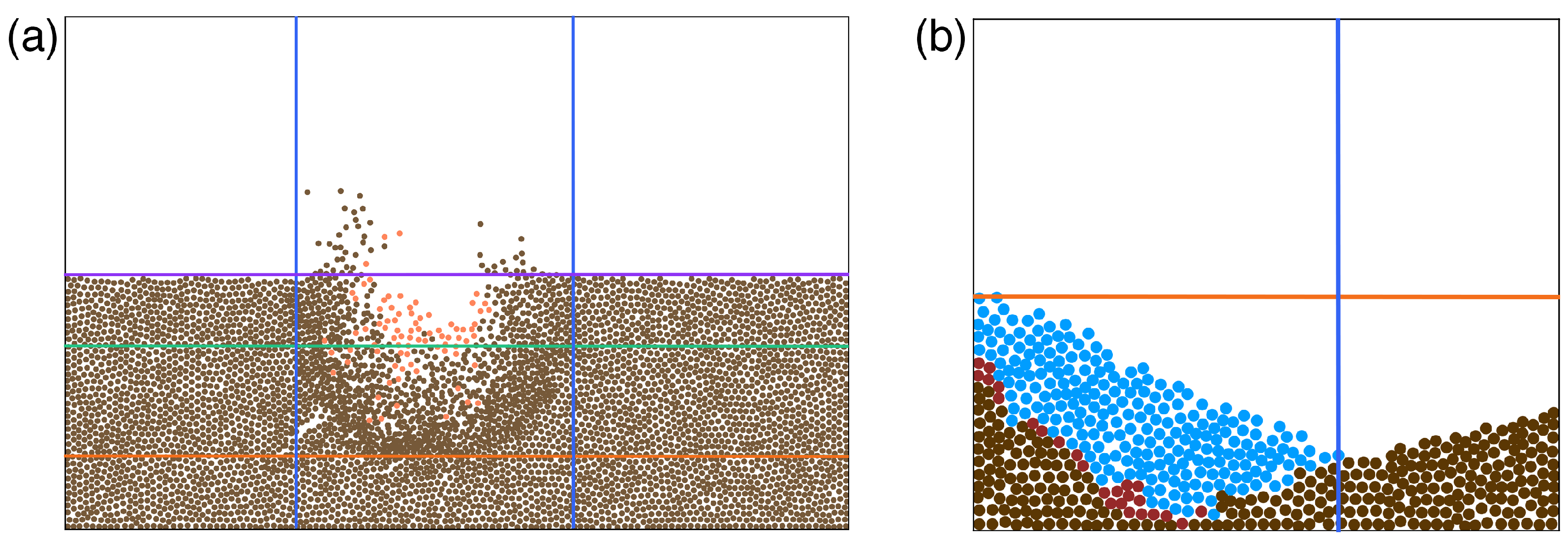
  • Imp Dep: impact depth. As the orange line in Figure 5a, the impact depth is the deepest depth caused by the meteorite impact. We measured this depth by statistical particle density.
  • Cra Dep: crater depth. As an auxiliary indicator for assessing impact depth, the crater depth refers to the vertical measurement of the crater. This measurement was determined by observing changes in the terrain, as illustrated by the green line in Figure 5a.
  • Imp R(L/R): impact range (left/right). As marked by the blue line in Figure 5a, the impact range represents the impact on the left and right sides in the horizontal direction caused by the impact. We measured them by judging the position change of particles.
  • Sp Num(L/R): number of splashed particles (left/right). We categorize particles situated above the ground as splashed particles. The purple line demarcated in Figure 5a signifies the ground level. Subsequently, we conducted a tally of the splashed particles on both the left and right sides.
  • Max Ht(L/R): max height of splash (left/right). The maximum height of splashed particles.
  • Mean Ht(L/R): mean height of splash (left/right). The average height of splashed particles.
Statics Problem. In this paper, we define the landslide body as the portion of soil or rock mass that is in the process of descending down the slope. It is represented as a cohesive mass of sliding particles, exemplified by the blue particles depicted in Figure 5b. The landslide tongue refers to a protruding, tongue-shaped formation that emerges at the leading edge of the landslide mass. Our primary emphasis lay in the evaluation of the shape characteristics of the landslide body, and we employed the following evaluation metrics for this purpose:
  • Slide Num: number of landslide body.
  • Max Ht: max height of landslide body. The height of the highest particle in the landslide body, as the orange line marked in Figure 5b.
  • Mean Ht: mean height of landslide body. The average height of the particles in the landslide body.
  • Tongue Dis: distance of landslide tongue. This indicator reflects the longest distance that the landslide tongue can reach, as the blue line marked in Figure 5b.
  • Dis: accuracy of landslide body. In order to further reflect the difference between the predicted particle position of the landslide body, denoted as P s , and the actual position, denoted as P s ^ , we calculated the Euclidean distance between the two:
    D ( P s ^ , P s ) = p i ^ P s ^ , p i P s ( x i ^ x i ) 2 + ( y i ^ y i ) 2 ,
    where p i ^ = ( x i ^ , y i ^ ) and p i = ( x i , y i ) .
Figure 5. (a): Moment of meteorite impact. (b): Onset of landslide. The lines with different colors indicate the measurement positions of different evaluation metrics.
Applsci 15 10432 g005
Principle Problem. The key point of the Direct Shear experiment was the position change of particles above and below the failure surface. We counted two items of data to reflect the accuracy of the model’s prediction of local (failure surface) and global (all) particle positions as follows:
  • Distance to Failure Surface (Above/Below): We calculated the Euclidean distance between the predicted particle position 5 mm above or below the failure surface, denoted as P f , and the actual position, denoted as P f ^ :
    D ( P f ^ , P f ) = p i ^ P f ^ , p i P f ( x i ^ x i ) 2 + ( y i ^ y i ) 2 + ( z i ^ z i ) 2 ,
    where p i ^ = ( x i ^ , y i ^ , z i ^ ) , and p i = ( x i , y i , z i ) .
  • Distance of All Particles: The calculation was the same as the above, except that the Euclidean distance of all particles was calculated.
Accuracy. In order to provide a visual representation of the accuracy of the predicted values for the evaluation metrics involved in the three experiments mentioned above, we calculated the accuracy of the metric, M , using the following formula:
A c c ( M ) = 1 | T | τ ϵ T ( 1 | M τ M τ ^ | M τ ) × 100 % ,
where T denotes a collection of time steps, and M τ and M τ ^ represent the evaluation metric derived from predictive values and ground truth, respectively, at time step τ .
Computational Efficiency. To assess the computational efficiency of Graph-DEM compared to the conventional discrete element method, we conducted measurements of the mean prediction time for our model and MatDEM, each executed on identical hardware components, including a NVIDIA GeForce RTX 3090 GPU, Intel Xeon 5218 CPU (Intel, Santa Clara, CA, USA), and 256 GB of memory.

5.3. Baselines

For a comprehensive assessment, we compared against (i) the conventional DEM (MatDEM) and (ii) recent DL/GNN-based particle simulators. On our three newly constructed datasets, we performed detailed comparisons with MatDEM to analyze advantages and limitations in terms of accuracy, generality, and efficiency. As an additional complement, on two public datasets, we followed prior benchmark protocols [52] and compared Graph-DEM with recent learning-based simulators, including the general models GNS [43] and MLP, conservation-law–based methods NNPhD [55] and LGNN [47], and equivariant approaches EGNN [48], GMN [49], ESTAG [50], and SGNN [51].

5.4. Experimental Setup

This section elaborates on the experimental setup in detail, including supplementary details of model implementation, data input and output, model parameter training process, experimental evaluation process, and relevant settings.

5.4.1. Model Implementation

The number of updater, Q, in P r o c e s s o r was set to 10. Additionally, the length of the node feature vector v i and edge feature vector e m was set to 128.
During the edge construction process, in order to quickly calculate the Euclidean distance between particles, we used the KD-Tree neighborhood algorithm [56]. For the three new constructed datasets, the hyperparameter R was set to 10 m, 10 m, 0.015 m in turn; for the public datasets, Slide-SameR and Slide-Small, R was set to 20 m.
Most hyperparameters followed prior work [43,52]; the remaining key settings were selected via parameter sensitivity analysis (see Appendix A). The implementation of the whole model was carried out using Pytorch 1.8.1 and Python 3.6.8.

5.4.2. Input and Output Details

We supplied our model with the particle positions P i t K + 1 : t and particle types T i . Specifically, for the Direct Shear and Slide-Small datasets, we additionally furnished the model with extra features f i (the Young’s modulus of soil particles, and the heterogeneous radii of slide particles) describing particle properties, as delineated in Table 1. These inputs were utilized in the construction of the node feature vector v i 0 and the edge feature vector e i j 0 .
Before feeding the network, interparticle relative distances were normalized by the contact radius (see Equation (7)); particle velocities and accelerations were standardized via z-scoring using the mean and standard deviation.
It should be noted that our input also included a mask, which assisted us in identifying particles of interest. As for the particles that were filtered out, such as the boundary particles responsible for ensuring particles did not escape the boundaries, and the particles constituting the shear box, their positional information was not a concern during the prediction phase since their positions could be readily obtained.
Overall, as specified in Equation (3), our model mapped particle attributes and recent trajectory states, X t K + 1 : t , to the next-step acceleration P ¨ t + 1 . Then, using Equation (1), we integrated this acceleration to obtain the velocity and position at time t + 1 , and by iterating this update (rollout) we predicted future trajectories. See Section 3.2 for details of this procedure.

5.4.3. Training

To accomplish the training of our model, we optimized the learnable parameter matrices within the model. Before describing the training process, it is imperative to first elucidate the procedure of parameter optimization.
Our model contained about 1.6 million parameters, through which we hoped to fit the laws of physics. Initially, these parameters were assigned random values. With training, they were gradually updated. For one prediction during the training phase, we denoted P ¨ as the predicted particle acceleration and P ¨ ^ as the truth of the particle acceleration. Then, we computed the L 2 loss on P ¨ , which can be described as:
L o s s ( P ¨ ^ , P ¨ ) = i = 1 N p ¨ ^ i p ¨ i 2 ,
where L o s s ( P ¨ ^ , P ¨ ) shows the difference between the predicted result and the truth. Since the parameters contain gradient information, the optimizer can optimize the parameters by gradient descent, which is the process of back-propagation [57].
For all experiments, we optimized model parameters with Adam [58] using a learning rate of 1 × 10 4 . Each simulation involved thousands of particles (Table 1), yielding large particle–contact graphs; accordingly, we trained on a single NVIDIA RTX 3090 (32 GB) with a batch size of 1. Training ran for 200 epochs with early stopping (patience = 30 ), and we monitored the validation loss and report the checkpoint that attained the best validation performance.
In order to carry out the optimization, the input data needed to include the truth P ¨ ^ . Therefore, a sample ( X t K + 1 : t , P ¨ ^ t + 1 ) contained a historical information sequence with the length of K and the truth in the next time step. For both the training and evaluation phases, the length of K was set to six.
We partitioned each dataset into three parts, with a ratio of 7:2:1 for training set, validation set, and test set, respectively. Among these, the training set was used to optimize parameters, the validation set was used to evaluate the performance of the current model in training to save the optimal set of parameters, and the test set was used to evaluate the model. Concretely, the splits were Meteorite Impact—672/192/97, Slide—700/199/101, Direct Shear—294/83/43, Slide-SameR—700/199/101, and Slide-Small—700/199/101.
Having comprehended the optimization procedure, let us now delve into the training process. For each training sample, we injected a small random-walk noise, N ( 0 , σ v 2 ) with σ v = 3 × 10 4 , into the input data to enhance robustness to noise and small state errors (accumulated error). Subsequently, the model generated prediction outcomes, and the loss function was computed to optimize the model parameters. This iterative process was reiterated until convergence, at which point the model was no longer amenable to further optimization. For the three datasets, we saved the optimal set of parameters for the next evaluation.

5.4.4. Evaluation

We used the samples in the test set to evaluate the performance of the model. Unlike the emphasis on the accuracy of one-step prediction in the training, the evaluation process paid more attention to predicting the complete trajectory of particles. Therefore, a sample ( X 1 : K , P ^ K : ) in the evaluation was composed of a historical information sequence starting from the first time step X 1 : K and a future particle trajectory P ^ K : . As mentioned in Section 3.2, our model does not predict the complete trajectory at once but predicts the particle position of each next time step through a cyclic update.
We loaded the previously saved optimal parameters for the evaluation. It is important to note that these parameters remained unchanged and unaltered during this process; they were solely employed for prediction purposes.

6. Results and Discussion

To demonstrate the versatility of Graph-DEM across various geotechnical problems and the capacity to adapt to different constitutive relationships, we present the results of three experiments conducted. Additionally, we provide an analysis of the computational time required to achieve these results and compare the prediction time of our model with the simulation time of conventional methods to explain the computational efficiency of our model.

6.1. Dynamics Problem

We evaluated the performance of Graph-DEM on the Meteorite Impact dataset by analyzing its overall effectiveness. Figure 6 demonstrates the predicted positions of particles by the model, highlighting the impact at various time steps, specifically, 1, 5, 10, 15, 20, and 30. Overall, the model performed well in accurately predicting and reconstructing the impact of the meteorite on the ground, ground deformation caused by the impact, and the effect of meteorite debris on the surrounding particles.
Moreover, to provide a quantitative analysis of the model’s performance, we measured the evaluation metrics outlined in Table 2. The results show that our predicted particle trajectories were almost identical to the actual trajectories. Through this evaluation, we aimed to gain further insights into the effectiveness of our model.
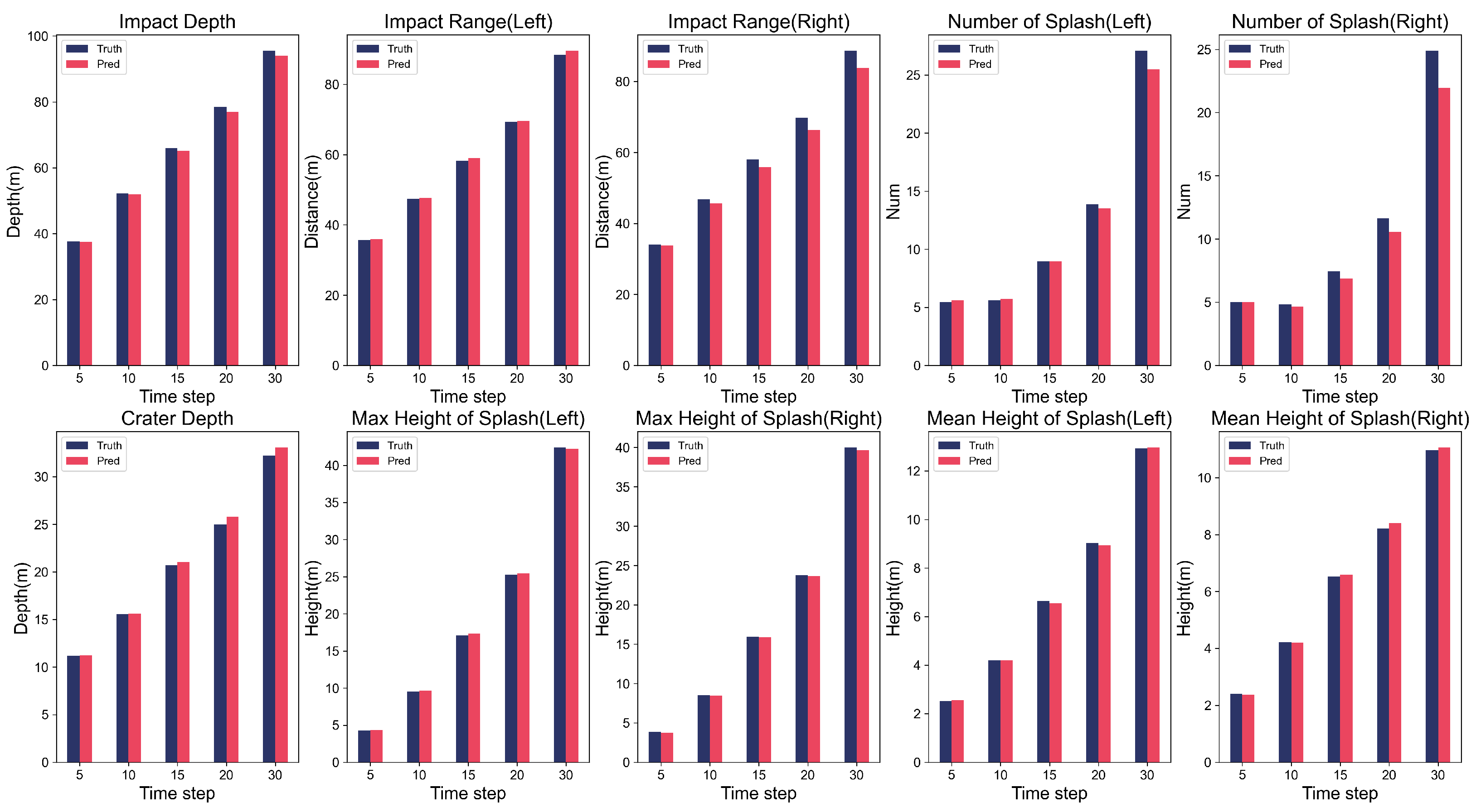
To make the contrast clearer, we also provide a data visualization in Figure 7. From the histograms, the deviation between the predicted value and the ground truth (MatDEM reference) for each metric at each future moment was small. At the same time, the change trend in various metrics was in line with physical expectations. As time progresses, the depth and range of the impact crater increased, and the number and height of splash particles also increased. However, compared with the classical DEM, since our surrogate simulation approximated particle–particle collisions at each step, some error accumulation over longer rollouts was observed; nevertheless, the overall accuracy remained above 93%.
As a supplement, we also simulated the process of meteorite impact with different velocities and directions and verified the speed sensitivity of the model. The results are shown in Figure 8. The craters formed by the impact have different shapes, which are well reflected by our model. This result also fully reflects the progressiveness nature of the model.
From the perspective of visual observation and data comparison, our model is accurate in predicting the impact process of a meteorite.

6.2. Statics Problem

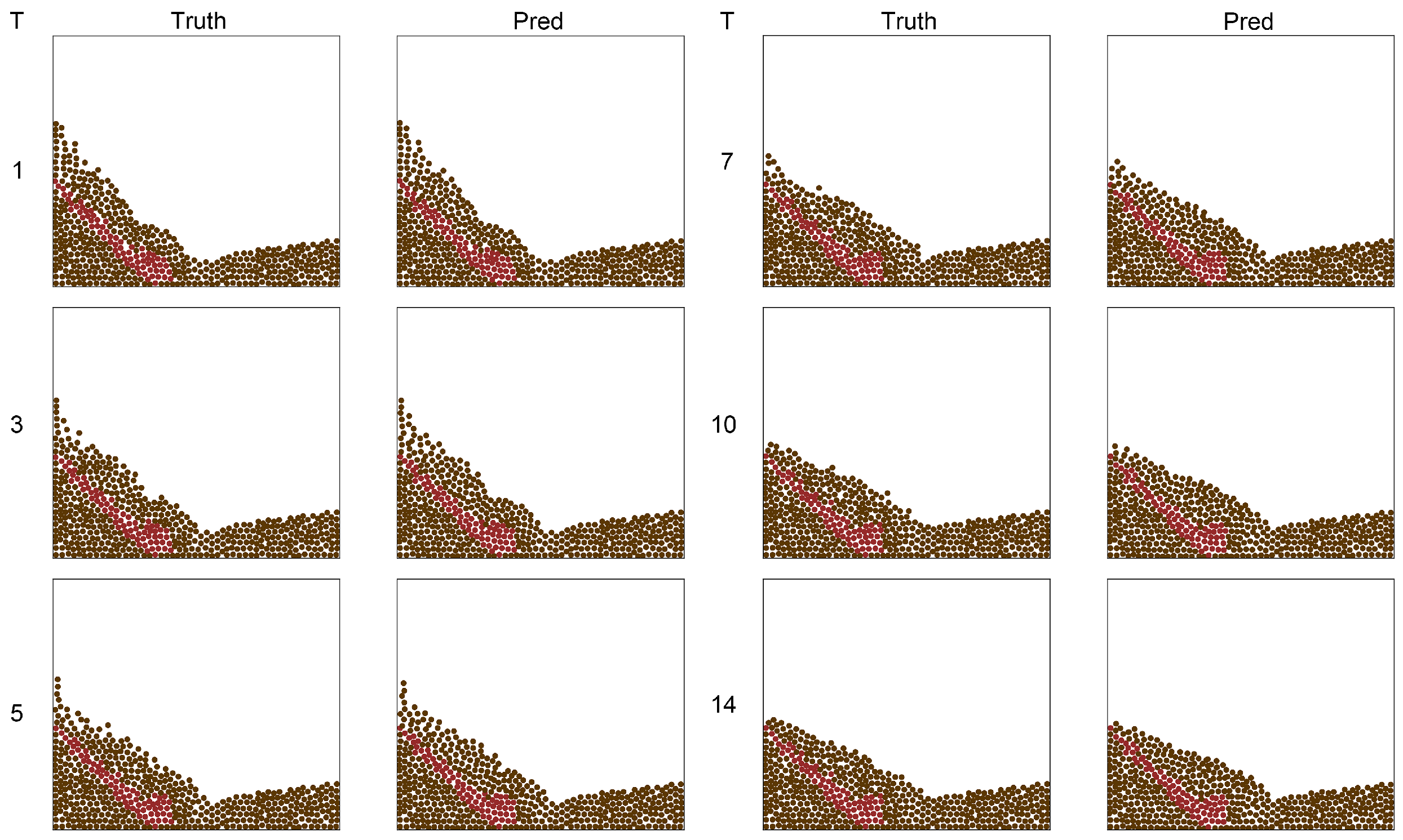
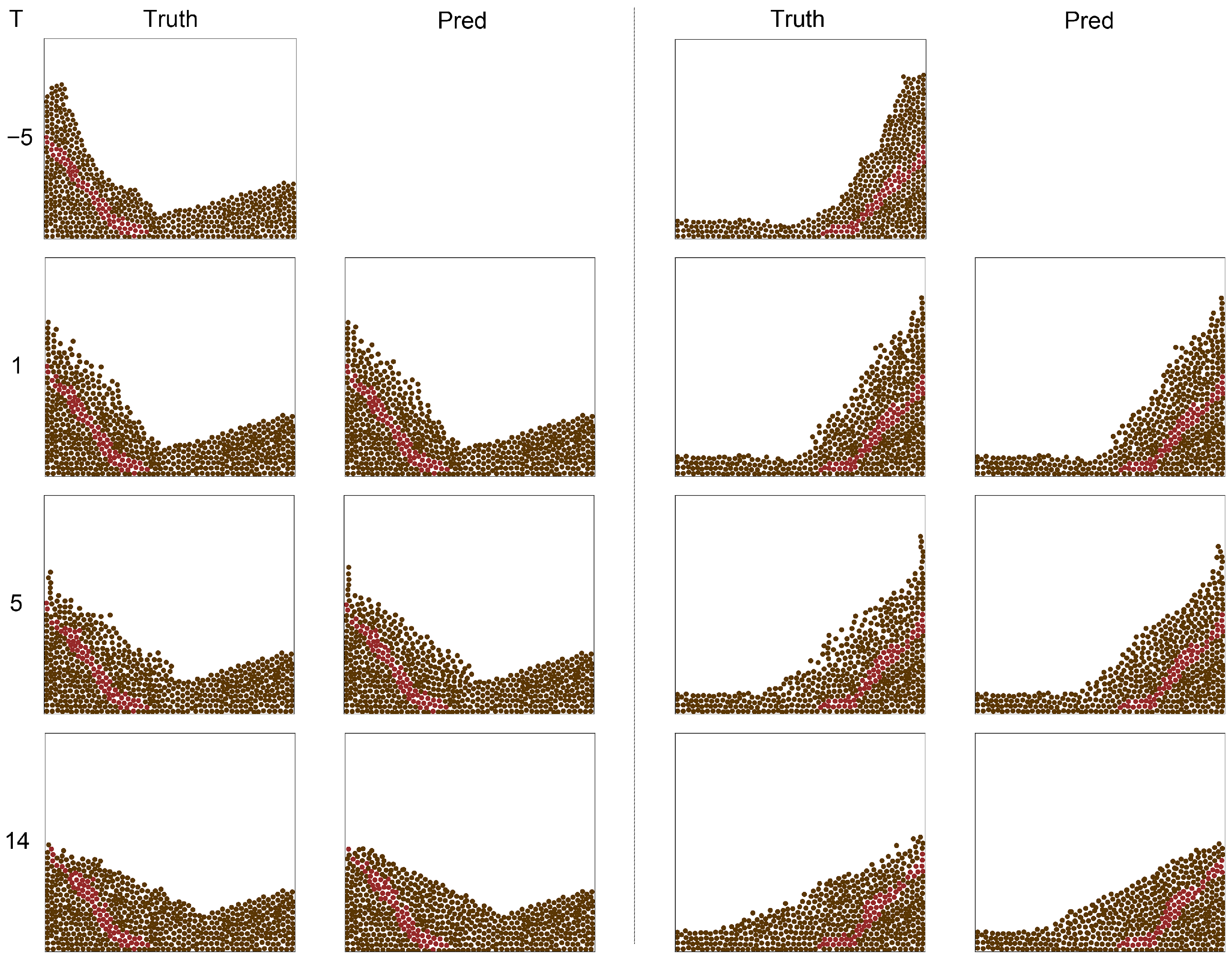
We utilized six historical time steps to forecast the future motion trajectory of particles in the Slide dataset. A sample’s entire motion trajectory, as illustrated in Figure 9, was presented by our model.
As a landslide develops and descends down the mountain, the landslide body gradually expands and the landslide tongue progressively elongates. Our model captured the overall trend and direction of the landslide accurately.
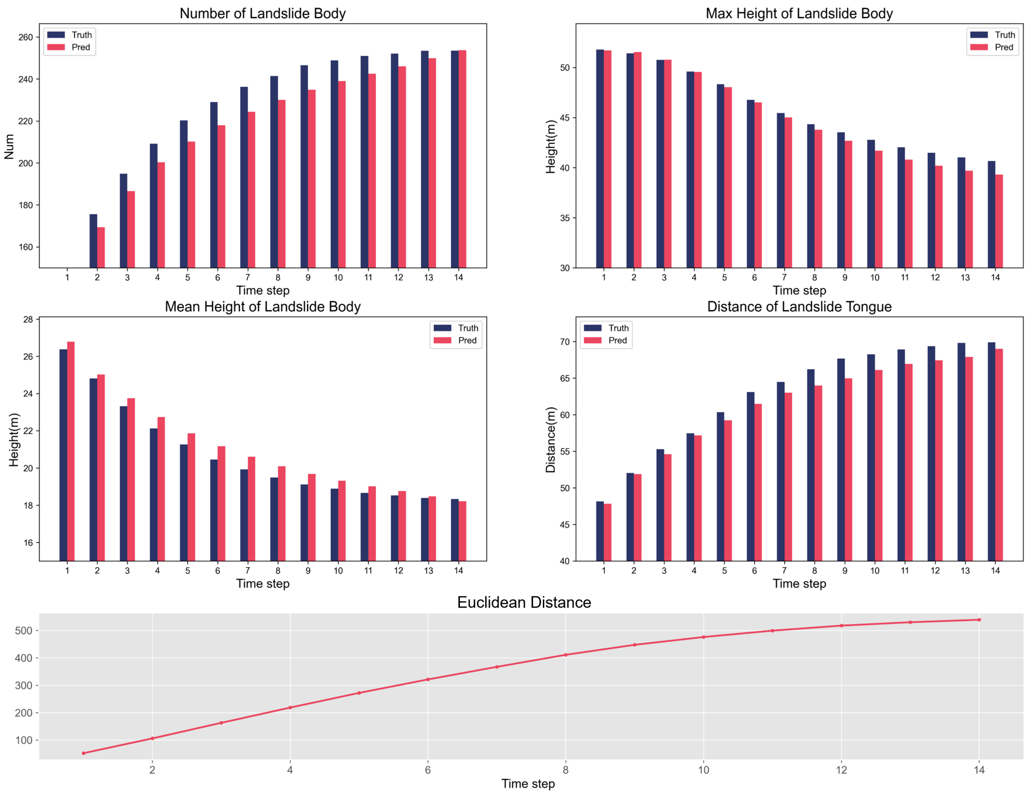
To evaluate the performance of our model, we employed various evaluation metrics and recorded the results in Table 3. Additionally, the measured results are graphically depicted in Figure 10 for better visualization.
Over time, the quantity of particles within the landslide steadily increased, concomitant with a decrease in the height of the landslide body and an extension of the landslide tongue. Overall, the evaluation metrics of predicted and true values were very close at all time steps. As time went on, the value of the Euclidean distance increased, indicating a reduction in the accuracy of particle position prediction within the model, as a result of accumulated errors. Compared with classical DEM, although our model’s predictions for the intermediate time steps could be slightly deficient and subject to error accumulation, its predictions of landslide features at the final time step were still relatively accurate. We believe this is due to the relative stability of the system in the later stages of the landslide, which facilitated the model’s understanding of landslide characteristics.
The set of figures (Figure 11) illustrates the predictive outcomes of the model on landslides of varying topographical features and soil stratification, highlighting the model’s compatibility with diverse scenarios.

6.3. Principle Problem

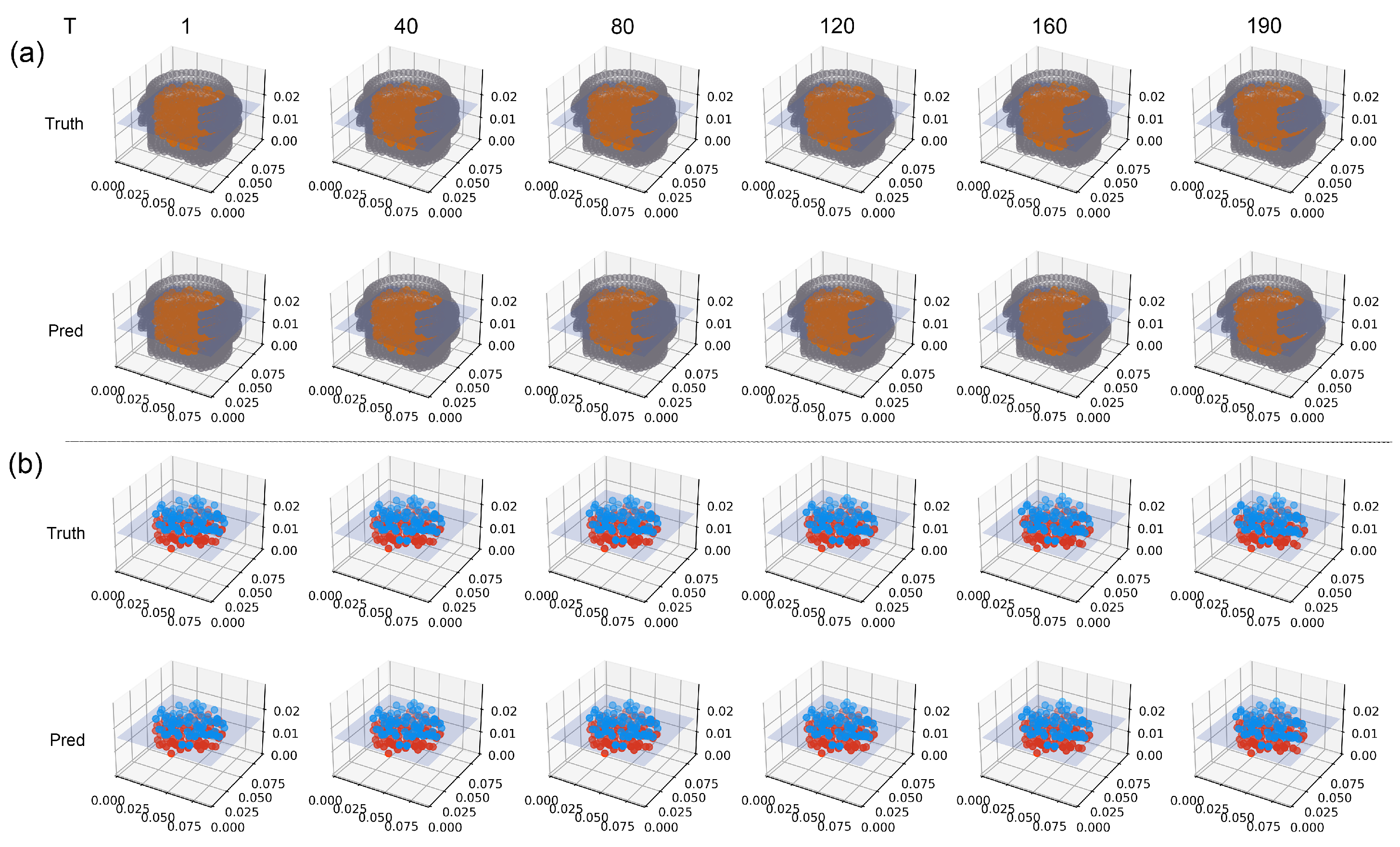
Next, we present the model’s prediction results for the Direct Shear test process. To illustrate the entire process of direct shearing, we selected schematic diagrams of the direct shearing process from different angles at the following time steps: 0, 40, 80, 120, 160, and 190. Figure 12 shows the particle trajectories of the 30% planed surface with the direct shear box, and the particle trajectories 5 mm above and below the failure surface. For clarity, we use blue particles to represent the particles above the failure surface and red particles to represent those below it. The light blue plane represents the failure surface. To further demonstrate the failure surface shape caused by direct shearing from multiple perspectives, we also provide a plan view and a top view as supplements in Figure 13.
In contrast to the other two datasets, particle displacements during direct shear were negligible. The most noticeable displacements occurred near the failure surface, for example, among particles above it, as seen from a frontal perspective. We can also examine particle spatial distributions from an overhead perspective and evaluate model predictions based on frontal features.
By visually observing the position and distribution of particles, we see that the model prediction was relatively accurate. In particular, the prediction of the shape and position of particles above and below the failure surface was close to the actual value. At the same time, no particle crossing occurred. As the direct shear box moved, the failure surface underwent relative displacement. The particles above and below it moved to the right with the direct shear box. In this process, they pulled each other and changed their relative positions, forming a mutual interlocking pattern.
To evaluate the accuracy of the model, we calculated the Euclidean distance between the predicted value and the actual value and recorded the results in Table 4. The Euclidean distance increased over time due to error accumulation. The particles below the failure surface had a larger error than those above it because of the movement of the direct shear box on the lower side.
We included the physical properties of particles in the input of the model. To test the model sensitivity to particle properties, we input particles with two different physical properties to the model and show the actual and predicted positions of the particles at the future 190th time step in Figure 14a,b. Since the difference in particle positions was not obvious, we calculated the mean values of particle positions in the x-direction and marked them on Figure 14a,b. The mean value of particle positions in (a) was smaller than that in (b) for both actual and predicted positions. To further compare the difference, we overlaid the two particle distributions and show them in Figure 14c, where (b) is on top and marked in gray. We can observe that the red part that is not covered by gray is exactly the difference between the two particle distributions. Both actual and predicted values show that (a) has a smaller mean value in the x-direction than (b). This consistent difference between actual and predicted values demonstrates the model sensitivity to particle property information. It also indicates the potential of the model for predicting complex and diverse particle trajectories.
By adjusting the input information, we can obtain a more general and feature-sensitive model that can be applied to different scenarios. However, this requires constructing a larger dataset to train the model.

6.4. Universality Across Different Constitutive Relations

The datasets corresponding to the aforementioned three experiments exhibit distinct constitutive relationships. Across these scenarios, our model demonstrated the capability to acquire relatively precise particle motion patterns and overarching motion trends. This underscores the adaptability inherent in our model framework to effectively learn diverse constitutive relationships.
This aptitude to accommodate various constitutive equations obviates the need for selecting appropriate constitutive relations and determining their parameters for individual cases. By furnishing accurate particle unit positions, such as those observed in real landslide processes, our model can directly learn, adjust, and assimilate the motion patterns between particles, by passing the conventional steps of constitutive equation selection and parameter determination.
Generalization to unseen scenarios. Other scenes typically obey the same local interaction principle: particles colliding with their nearest neighbors. Graph-DEM makes this locality explicit by constructing a particle–contact graph and learning the collision-driven state update via neural message passing. Because this pipeline (graph construction + message-passing update) is scenario-agnostic and unchanged across tasks, the model adapts rapidly to new scenes without redesigning the architecture or loss. Additionally, for particles with additional physical properties, we encode these attributes in the node features (and, when available, in edge features) or attach a discrete-type indicator to distinguish heterogeneous materials and constitutive behaviors.
Applicability to real-world data. When real systems are recorded as particle identities and trajectories, Graph-DEM can be applied directly with no architectural modifications, since it fits observed interparticle motions rather than hand-crafted constitutive laws. The strong results on DEM benchmarks—which closely approximate physical interactions—indicate that the same model is naturally transferable to real granular datasets of the same format.

6.5. Computational Efficiency

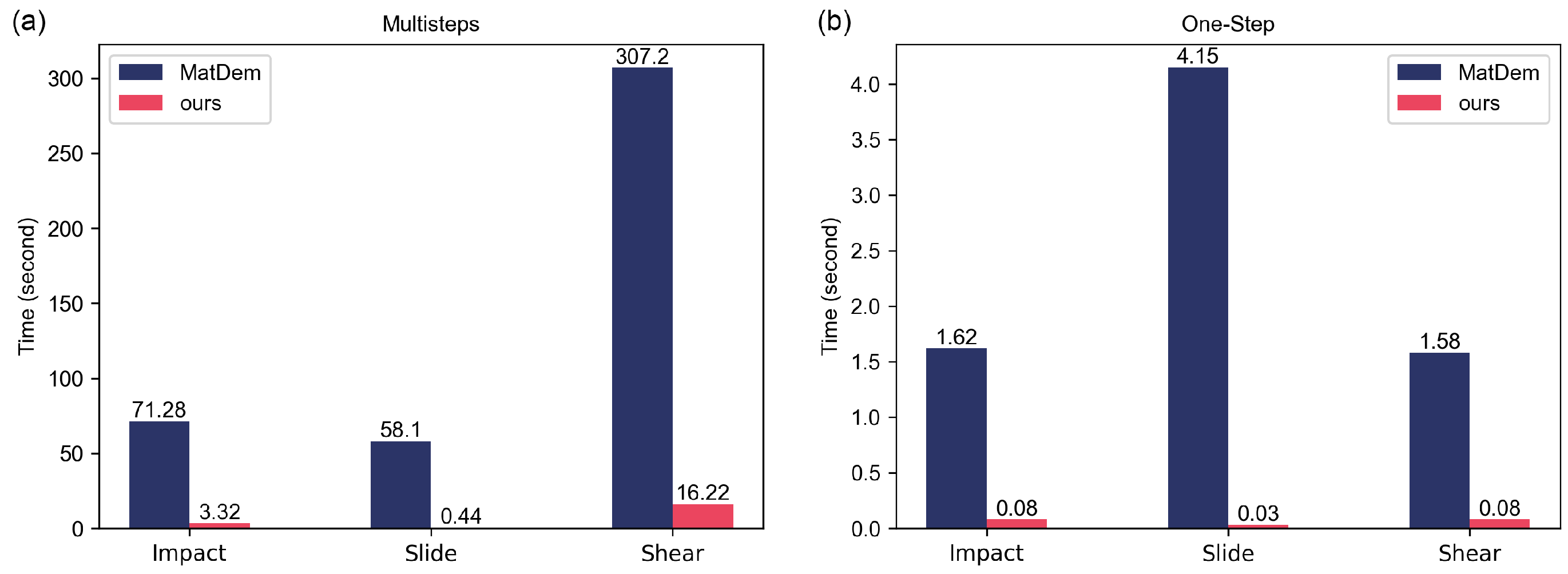
After showcasing the accuracy of our model and the universality of the framework across various scenarios, we proceed to compare the prediction time of Graph-DEM and MatDEM for the complete trajectories of particles in each dataset. Figure 15a shows the comparison for 44 time steps for the Meteorite Impact dataset, 14 time steps for landslide prediction, and 194 time steps for direct shear prediction. Figure 15b shows the time comparison when calculating one step. Both multiple steps and one step show a significant increase in computational efficiency (up to 90%), with a remarkable 99% improvement observed on the landslide simulation, which illustrates the advantages of our model in terms of prediction speed and computational efficiency.
We also report the time cost of model training in Table 5. For a single prediction task, the traditional discrete element method has a time advantage. However, our model has more generality and a time advantage for repeated prediction tasks.

6.6. Further Comparisons and Discussion

To further substantiate the advantages of our approach, we compared Graph-DEM with both conventional DEM and GNN-based particle dynamics methods in detail.

6.6.1. Comparison with Conventional DEM

Relative to the conventional DEM, our method offers the following advantages:
  • Efficiency. As a learned surrogate, Graph-DEM delivers substantial wall-clock speedups by replacing costly contact search and force integration with parallel neural inference.
  • Generality. The framework is agnostic to specific scenarios and can proxy multiple granular phenomena under a unified graph formulation.
  • Accuracy. Against DEM references (ground truth), Graph-DEM attains an accuracy above 93% on multiple metrics across datasets.
These benefits stem from directly learning the state-to-state mapping of particle interactions via message passing on a particle–contact graph (nodes as particles, edges as contacts), thereby avoiding the complex and often inefficient mathematical computations required by the classical DEM.
Limitations. The surrogate nature of Graph-DEM also entails trade-offs. First, because it bypasses strict analytical derivations, small approximation errors are inevitable and can accumulate over long rollouts; thus, predictions cannot be 100% exact. Second, scalability is currently bounded by GPU memory: on a single 24 GB GPU, practical graphs typically contain on the order of 2 × 10 4 particles. While larger memories or multi-GPU setups can raise this ceiling, real-world or ultra-large systems may require spatial decomposition (subgraph batching/tiling) to simulate trajectories in parts and then compose the results.

6.6.2. Comparison with Related DL-Based Methods

To further validate Graph-DEM, we compared it with related deep-learning (including GNN-based) simulators on the two public datasets Slide-SameR and Slide-Small; MSE results are summarized in Table 6, where numbers follow the benchmark in [52], and the best scores are bolded. The main observations are as follows:
(i) First-tier performance. Graph-DEM attained first-tier results against all baselines. We attribute this to its flexible, editable framework, which adapts quickly across scenarios—for example, by encoding the non-uniform radii of Slide-Small as node features—thereby outperforming general-purpose simulators such as GNS.
(ii) Limits of additional constraints. Methods enforcing conservation laws or strict equivariance (e.g., LGNN, EGNN) often underperform here, as real granular systems are dissipative and exhibit gravity-induced asymmetry that violates these assumptions. In contrast, Graph-DEM imposes no such constraints; instead, it learns collision-driven state updates via message passing on the particle–contact graph from observed pre-/post-collision states, enabling robust adaptation across scenarios.
Limitations. Graph-DEM is a simple, general framework; its adaptability to highly specialized structures or particle properties warrants further study. In this study, our goal was to assess the efficiency and generality of GNN-based surrogates for DEMs. Improving accuracy via stronger physics priors (e.g., embedded mechanics or data-driven physical constraints) is left as future work.

7. Conclusions

This paper presented Graph-DEM, which uses graph neural networks instead of traditional discrete element computation for physics particle trajectory simulation. Our model consists of three components: a constructor that builds a graph structure and characterizes particle attributes and relations, a processor that fits the interaction patterns between particles, and a generator that predicts potential motion trends.
To demonstrate the effectiveness, universality, and efficiency of the model, we conducted three representative experiments: meteorite impact simulation, landslide simulation, and direct shear experiment simulation. In the first two experiments, all performance metrics achieved an accuracy of over 93%, with most falling between 96% and 100%. As a supplementary evaluation, we utilized the Euclidean distance to assess the accuracy of predicted particle positions. Furthermore, the three representative experiments encompassed different constitutive relations, encompassing both two-dimensional and three-dimensional data, thereby reflecting the universality of our model and its adaptability to different constitutive equations. Crucially, based on this acceptable prediction accuracy, the computational efficiency of the model was improved by at least 90%, with a remarkable 99% improvement observed on the landslide simulation.
In the near future, this model can be a key method for optimizing the computational efficiency of discrete elements. Moreover, due to the structural advantages of the model, it has scalability and flexibility to handle complex scenarios in the future. Such scenarios include but are not limited to particle attribute complexity, particle radius complexity, and particle type complexity.
Nonetheless, research into using neural networks to replace traditional numerical calculations is still in its infancy. From the data side, studying how to represent real rock and soil bodies into discrete particles and converting them into coordinates as input will help to better simulate real physics; from the model side, how to use limited resources to simulate a larger number of particles will also be the main direction of research.

Author Contributions

Methodology, B.L., K.C., and J.Y.; software, B.L.; data curation, B.L. and K.L.; writing—original draft preparation, B.L.; writing—review and editing, J.Y., J.F., and X.C.; funding acquisition, B.D. All authors have read and agreed to the published version of the manuscript.

Funding

This work was supported by the National Key R&D Program of China under Grant 2023YFB2603605, the National Natural Science Foundation of China under Grant No. U2469205, the Fundamental Research Funds for the Central Universities of China under Grant No. JKF-20240769, and the Beijing Nova Program under Grant No. 20230484353.

Institutional Review Board Statement

Not applicable.

Informed Consent Statement

Not applicable.

Data Availability Statement

All data and codes that support the findings of this study will be available and made public if this paper is accepted.

Conflicts of Interest

The authors declare no conflicts of interest.

Appendix A. Hyperparameter Sensitivity Analysis

To choose appropriate hyperparameters, we followed prior work [43,52] to define plausible search ranges on our data and then conducted a grid search within those ranges. We report three key settings—message-passing iterations (Q), contact radius (R), and node/edge vector length (hidden size)—with summary full-rollout MSE results for the three datasets in Table A1. Other hyperparameters were kept at values commonly used in the literature [43,52].
Message-passing iterations ( Q ). Q controls how deeply a node aggregates collision information from its neighbors. We evaluated Q { 5 , 10 , 15 } . With too few iterations, a center node cannot sufficiently integrate multiple neighbor interactions; with too many, the added computation provides diminishing returns and increases overhead. We therefore selected Q = 10 , which yielded the best overall trade-off.
Contact radius ( R ). R determines the ε -ball neighborhood used to create edges. If R is too small, graphs become sparsely connected (or even edge-free), preventing effective collision modeling; if R is too large, many non-colliding pairs are linked, wasting computation. Guided by particle radii and empirical tests, we adopted R = 10   m (Meteorite Impact), R = 10   m (Slide), and R = 0.015   m (Direct Shear).
Vector length (hidden size). The hidden size governs the model’s expressive capacity. We tested { 64 , 128 , 256 } . While 256 can be slightly better on some datasets, it increases runtime and memory. Balancing accuracy and efficiency, we set both node and edge feature dimensions to 128.
Table A1. Hyperparameter sensitivity analysis (MSE ↓).
Meteorite ImpactSlideDirect Shear ( × 10 8 )
Q=57.732=53.887=511.851
=106.931=102.305=107.419
=157.193=152.806=157.712
R=135.028=128.365=0.001858.752
=87.506=82.839=0.0110.138
=106.931=102.305=0.0157.419
=127.012=122.337=0.027.808
Vector Length=648.082=643.068=648.730
=1286.931=1282.305=1287.419
=2566.807=2562.358=2567.862

References

  1. Cundall, P.A.; Strack, O.D. A discrete numerical model for granular assemblies. Geotechnique 1979, 29, 47–65. [Google Scholar] [CrossRef]
  2. Liu, C. Matrix Discrete Element Analysis of Geological and Geotechnical Engineering; Springer: Berlin/Heidelberg, Germany, 2021. [Google Scholar] [CrossRef]
  3. Elman, J.L. Finding structure in time. Cogn. Sci. 1990, 14, 179–211. [Google Scholar] [CrossRef]
  4. Krizhevsky, A.; Sutskever, I.; Hinton, G.E. Imagenet classification with deep convolutional neural networks. Commun. ACM 2017, 60, 84–90. [Google Scholar] [CrossRef]
  5. Scarselli, F.; Gori, M.; Tsoi, A.C.; Hagenbuchner, M.; Monfardini, G. The graph neural network model. IEEE Trans. Neural Netw. 2008, 20, 61–80. [Google Scholar] [CrossRef] [PubMed]
  6. Bruna, J.; Zaremba, W.; Szlam, A.; LeCun, Y. Spectral networks and locally connected networks on graphs. arXiv 2013, arXiv:1312.6203. [Google Scholar] [CrossRef]
  7. Vaswani, A.; Shazeer, N.; Parmar, N.; Uszkoreit, J.; Jones, L.; Gomez, A.N.; Kaiser, Ł.; Polosukhin, I. Attention is all you need. In Advances in Neural Information Processing Systems; Curran Associates Inc.: Red Hook, NY, USA, 2017; Volume 30. [Google Scholar]
  8. Zhang, W.; Li, H.; Tang, L.; Gu, X.; Wang, L.; Wang, L. Displacement prediction of Jiuxianping landslide using gated recurrent unit (GRU) networks. Acta Geotech. 2022, 17, 1367–1382. [Google Scholar] [CrossRef]
  9. Wang, Z.Z.; Goh, S.H. A maximum entropy method using fractional moments and deep learning for geotechnical reliability analysis. Acta Geotech. 2022, 17, 1147–1166. [Google Scholar] [CrossRef]
  10. Guo, D.; Li, J.; Jiang, S.H.; Li, X.; Chen, Z. Intelligent assistant driving method for tunnel boring machine based on big data. Acta Geotech. 2022, 17, 1019–1030. [Google Scholar] [CrossRef]
  11. Kipf, T.N.; Welling, M. Semi-supervised classification with graph convolutional networks. arXiv 2016, arXiv:1609.02907. [Google Scholar] [CrossRef]
  12. Gilmer, J.; Schoenholz, S.S.; Riley, P.F.; Vinyals, O.; Dahl, G.E. Neural message passing for quantum chemistry. In Proceedings of the International Conference on Machine Learning, Sydney, Australia, 6–11 August 2017; pp. 1263–1272. [Google Scholar]
  13. Hornik, K.; Stinchcombe, M.; White, H. Multilayer feedforward networks are universal approximators. Neural Netw. 1989, 2, 359–366. [Google Scholar] [CrossRef]
  14. LeCun, Y.; Bengio, Y.; Hinton, G. Deep learning. Nature 2015, 521, 436–444. [Google Scholar] [CrossRef] [PubMed]
  15. Utili, S.; Nova, R. DEM analysis of bonded granular geomaterials. Int. J. Numer. Anal. Methods Geomech. 2008, 32, 1997–2031. [Google Scholar] [CrossRef]
  16. Krzaczek, M.; Nitka, M.; Tejchman, J. Modelling of Hydraulic Fracturing in Rocks in Non-isothermal Conditions Using Coupled DEM/CFD Approach with Two-Phase Fluid Flow Model. In Multiscale Processes of Instability, Deformation and Fracturing in Geomaterials, Proceedings of the 12th International Workshop on Bifurcation and Degradation in Geomechanics; Springer: Cham, Switzerland, 2022; pp. 114–126. [Google Scholar] [CrossRef]
  17. El Shamy, U.; Abdelhamid, Y. Modeling granular soils liquefaction using coupled lattice Boltzmann method and discrete element method. Soil Dyn. Earthq. Eng. 2014, 67, 119–132. [Google Scholar] [CrossRef]
  18. Cai, M.; Kaiser, P.; Morioka, H.; Minami, M.; Maejima, T.; Tasaka, Y.; Kurose, H. FLAC/PFC coupled numerical simulation of AE in large-scale underground excavations. Int. J. Rock Mech. Min. Sci. 2007, 44, 550–564. [Google Scholar] [CrossRef]
  19. O’Sullivan, C. Particulate Discrete Element Modelling: A Geomechanics Perspective; CRC Press: Boca Raton, FL, USA, 2011. [Google Scholar]
  20. Wang, X.; Ji, H.; Shi, C.; Wang, B.; Ye, Y.; Cui, P.; Yu, P.S. Heterogeneous graph attention network. In Proceedings of the World Wide Web Conference, San Francisco, CA, USA, 13–17 May 2019; pp. 2022–2032. [Google Scholar] [CrossRef]
  21. Qu, L.; Zhu, H.; Duan, Q.; Shi, Y. Continuous-time link prediction via temporal dependent graph neural network. In Proceedings of the Web Conference 2020, Taipei, Taiwan, 20–24 April 2020; pp. 3026–3032. [Google Scholar] [CrossRef]
  22. Velickovic, P.; Cucurull, G.; Casanova, A.; Romero, A.; Lio, P.; Bengio, Y. Graph attention networks. arXiv 2017, arXiv:1710.10903. [Google Scholar] [CrossRef]
  23. Wu, Z.; Pan, S.; Long, G.; Jiang, J.; Chang, X.; Zhang, C. Connecting the dots: Multivariate time series forecasting with graph neural networks. In Proceedings of the 26th ACM SIGKDD International Conference on Knowledge Discovery & Data Mining, Virtual Event, 6–10 July 2020; pp. 753–763. [Google Scholar] [CrossRef]
  24. Zhang, M.; Chen, Y. Link prediction based on graph neural networks. In Advances in Neural Information Processing Systems; Curran Associates Inc.: Red Hook, NY, USA, 2018; Volume 31. [Google Scholar]
  25. Nasiri, E.; Berahmand, K.; Rostami, M.; Dabiri, M. A novel link prediction algorithm for protein-protein interaction networks by attributed graph embedding. Comput. Biol. Med. 2021, 137, 104772. [Google Scholar] [CrossRef]
  26. Zhou, J.; Cui, G.; Hu, S.; Zhang, Z.; Yang, C.; Liu, Z.; Wang, L.; Li, C.; Sun, M. Graph neural networks: A review of methods and applications. AI Open 2020, 1, 57–81. [Google Scholar] [CrossRef]
  27. Li, Y.; Yu, R.; Shahabi, C.; Liu, Y. Diffusion convolutional recurrent neural network: Data-driven traffic forecasting. arXiv 2017, arXiv:1707.01926. [Google Scholar] [CrossRef]
  28. Yu, B.; Yin, H.; Zhu, Z. Spatio-temporal graph convolutional networks: A deep learning framework for traffic forecasting. arXiv 2017, arXiv:1709.04875. [Google Scholar] [CrossRef]
  29. Duvenaud, D.K.; Maclaurin, D.; Iparraguirre, J.; Bombarell, R.; Hirzel, T.; Aspuru-Guzik, A.; Adams, R.P. Convolutional networks on graphs for learning molecular fingerprints. In Advances in Neural Information Processing Systems; MIT Press: Cambridge, MA, USA, 2015; Volume 28. [Google Scholar]
  30. Schlichtkrull, M.; Kipf, T.N.; Bloem, P.; Van Den Berg, R.; Titov, I.; Welling, M. Modeling relational data with graph convolutional networks. In The Semantic Web: 15th International Conference, ESWC 2018, Heraklion, Crete, Greece, 3–7 June 2018; Proceedings 15; Springer: Cham, Switzerland, 2018; pp. 593–607. [Google Scholar]
  31. Ying, R.; He, R.; Chen, K.; Eksombatchai, P.; Hamilton, W.L.; Leskovec, J. Graph convolutional neural networks for web-scale recommender systems. In Proceedings of the 24th ACM SIGKDD International Conference on Knowledge Discovery & Data Mining, London, UK, 19–23 August 2018; pp. 974–983. [Google Scholar] [CrossRef]
  32. He, X.; Deng, K.; Wang, X.; Li, Y.; Zhang, Y.; Wang, M. Lightgcn: Simplifying and powering graph convolution network for recommendation. In Proceedings of the 43rd International ACM SIGIR Conference on Research and Development in Information Retrieval, Virtual Event, 25–30 July 2020; pp. 639–648. [Google Scholar] [CrossRef]
  33. Grzeszczuk, R.; Terzopoulos, D.; Hinton, G. Neuroanimator: Fast neural network emulation and control of physics-based models. In Proceedings of the 25th Annual Conference on Computer Graphics and Interactive Techniques, Orlando, FL, USA, 19–24 July 1998; pp. 9–20. [Google Scholar] [CrossRef]
  34. Chern, A.; Knöppel, F.; Pinkall, U.; Schröder, P. Inside fluids: Clebsch maps for visualization and processing. ACM Trans. Graph. (TOG) 2017, 36, 142. [Google Scholar] [CrossRef]
  35. Wu, K.; Truong, N.; Yuksel, C.; Hoetzlein, R. Fast fluid simulations with sparse volumes on the GPU. Comput. Graph. Forum 2018, 37, 157–167. [Google Scholar] [CrossRef]
  36. Skrivan, T.; Soderstrom, A.; Johansson, J.; Sprenger, C.; Museth, K.; Wojtan, C. Wave curves: Simulating lagrangian water waves on dynamically deforming surfaces. ACM Trans. Graph. (TOG) 2020, 39, 65. [Google Scholar] [CrossRef]
  37. Wolper, J.; Fang, Y.; Li, M.; Lu, J.; Gao, M.; Jiang, C. CD-MPM: Continuum damage material point methods for dynamic fracture animation. ACM Trans. Graph. (TOG) 2019, 38, 119. [Google Scholar] [CrossRef]
  38. Fei, Y.; Batty, C.; Grinspun, E.; Zheng, C. A multi-scale model for simulating liquid-fabric interactions. ACM Trans. Graph. (TOG) 2018, 37, 51. [Google Scholar] [CrossRef]
  39. Ruan, L.; Liu, J.; Zhu, B.; Sueda, S.; Wang, B.; Chen, B. Solid-fluid interaction with surface-tension-dominant contact. ACM Trans. Graph. (TOG) 2021, 40, 120. [Google Scholar] [CrossRef]
  40. Ladickỳ, L.; Jeong, S.; Solenthaler, B.; Pollefeys, M.; Gross, M. Data-driven fluid simulations using regression forests. ACM Trans. Graph. (TOG) 2015, 34, 199. [Google Scholar] [CrossRef]
  41. Li, Y.; Wu, J.; Tedrake, R.; Tenenbaum, J.B.; Torralba, A. Learning particle dynamics for manipulating rigid bodies, deformable objects, and fluids. arXiv 2018, arXiv:1810.01566. [Google Scholar] [CrossRef]
  42. Ummenhofer, B.; Prantl, L.; Thuerey, N.; Koltun, V. Lagrangian fluid simulation with continuous convolutions. In Proceedings of the International Conference on Learning Representations, Addis Ababa, Ethiopia, 26–30 April 2020; Available online: https://openreview.net/forum?id=B1lDoJSYDH (accessed on 20 September 2025).
  43. Sanchez-Gonzalez, A.; Godwin, J.; Pfaff, T.; Ying, R.; Leskovec, J.; Battaglia, P. Learning to simulate complex physics with graph networks. In Proceedings of the International Conference on Machine Learning, Virtual, 13–18 July 2020; pp. 8459–8468. [Google Scholar]
  44. Rubanova, Y.; Sanchez-Gonzalez, A.; Pfaff, T.; Battaglia, P. Constraint-based graph network simulator. arXiv 2021, arXiv:2112.09161. [Google Scholar] [CrossRef]
  45. Wu, T.; Wang, Q.; Zhang, Y.; Ying, R.; Cao, K.; Sosic, R.; Jalali, R.; Hamam, H.; Maucec, M.; Leskovec, J. Learning large-scale subsurface simulations with a hybrid graph network simulator. In Proceedings of the 28th ACM SIGKDD Conference on Knowledge Discovery and Data Mining, Washington, DC, USA, 14–18 August 2022; pp. 4184–4194. [Google Scholar] [CrossRef]
  46. Cranmer, M.; Greydanus, S.; Hoyer, S.; Battaglia, P.; Spergel, D.; Ho, S. Lagrangian neural networks. arXiv 2020, arXiv:2003.04630. [Google Scholar]
  47. Bhattoo, R.; Ranu, S.; Krishnan, N. Learning articulated rigid body dynamics with lagrangian graph neural network. In Advances in Neural Information Processing Systems; Curran Associates Inc.: Red Hook, NY, USA, 2022; Volume 35, pp. 29789–29800. [Google Scholar]
  48. Satorras, V.G.; Hoogeboom, E.; Welling, M. E(n) equivariant graph neural networks. In Proceedings of the International Conference on Machine Learning, Virtual, 18–24 July 2021; pp. 9323–9332. [Google Scholar]
  49. Huang, W.; Han, J.; Rong, Y.; Xu, T.; Sun, F.; Huang, J. Equivariant graph mechanics networks with constraints. arXiv 2022, arXiv:2203.06442. [Google Scholar] [CrossRef]
  50. Wu, L.; Hou, Z.; Yuan, J.; Rong, Y.; Huang, W. Equivariant spatio-temporal attentive graph networks to simulate physical dynamics. In Advances in Neural Information Processing Systems; Curran Associates Inc.: Red Hook, NY, USA, 2023; Volume 36, pp. 45360–45380. [Google Scholar]
  51. Han, J.; Huang, W.; Ma, H.; Li, J.; Tenenbaum, J.; Gan, C. Learning physical dynamics with subequivariant graph neural networks. In Advances in Neural Information Processing Systems; Curran Associates Inc.: Red Hook, NY, USA, 2022; Volume 35, pp. 26256–26268. [Google Scholar]
  52. Li, B.; Du, B.; Ye, J.; Huang, J.; Sun, L.; Feng, J. Learning solid dynamics with graph neural network. Inf. Sci. 2024, 676, 120791. [Google Scholar] [CrossRef]
  53. Glorot, X.; Bengio, Y. Understanding the difficulty of training deep feedforward neural networks. In Proceedings of the Thirteenth International Conference on Artificial Intelligence and Statistics, Sardinia, Italy, 13–15 May 2010; pp. 249–256. Available online: http://proceedings.mlr.press/v9/glorot10a (accessed on 20 September 2025).
  54. Ba, J.L.; Kiros, J.R.; Hinton, G.E. Layer normalization. arXiv 2016, arXiv:1607.06450. [Google Scholar] [CrossRef]
  55. Liu, Z.; Wang, B.; Meng, Q.; Chen, W.; Tegmark, M.; Liu, T.Y. Machine-learning nonconservative dynamics for new-physics detection. Phys. Rev. E 2021, 104, 055302. [Google Scholar] [CrossRef] [PubMed]
  56. Arya, S.; Mount, D.M.; Netanyahu, N.S.; Silverman, R.; Wu, A.Y. An optimal algorithm for approximate nearest neighbor searching fixed dimensions. J. ACM (JACM) 1998, 45, 891–923. [Google Scholar] [CrossRef]
  57. Rumelhart, D.E.; Hinton, G.E.; Williams, R.J. Learning representations by back-propagating errors. Nature 1986, 323, 533–536. [Google Scholar] [CrossRef]
  58. Kingma, D.P.; Ba, J. Adam: A method for stochastic optimization. arXiv 2014, arXiv:1412.6980. [Google Scholar] [CrossRef]
Figure 1. Topological structure similarity between a graph and the discrete element method. (a) The distribution of particle positions. (b) The “particle-spring” topology in the linear contact model. (c) The topological structure of graph neural networks.
Applsci 15 10432 g001
Figure 2. The architecture of Graph-DEM. In order to facilitate understanding, we use yellow tags to represent node feature vectors and green tags to represent edge feature vectors. Data flow between different components is completed through these tags. Nodes with different colors represent different particle types.
Applsci 15 10432 g002
Figure 3. Architecture of the updater. The update process of edge feature vectors is shown in the purple area. We select the edge feature vector e i j q and the two node feature vectors corresponding to this edge, v i q and v j q , to participate in the calculation and obtain the updated edge feature vector e i j q hoping to simulate the effect of the neighboring particle v i on the central particle v j . On the other hand, the update process for the node feature vectors is executed in the orange area. Here, we synthesize the effects of neighboring particles and convert them into the node feature vectors, v j q + 1 .
Applsci 15 10432 g003
Figure 4. Architecture of the MLP. For input vector I R k i , it passes through three linear layers with 128 neurons, including a ReLU activation function between the linear layers, and passes through LayerNorm before the output. In the end, I is projected onto a k o -dimensional vector space.
Applsci 15 10432 g004
Figure 6. Prediction of the meteorite impact process. The orange particles represent the meteorite, and the brown particles represent the ground. The true and predicted positions of the particles at future time steps 1, 5, 10, 15, 20, and 30 are shown.
Applsci 15 10432 g006
Figure 7. Evaluation metrics visualization of the Meteorite Impact dataset: comparison of truth value and predicted value under different time steps.
Applsci 15 10432 g007
Figure 8. Different shapes of impact craters formed by three meteorites with different directions and velocities. The true and predicted positions of the particles at start time step (−5) and future time steps 1, 15, and 40 are shown.
Applsci 15 10432 g008
Figure 9. Landslide process. The red particles indicate those that are likely to slide, while the brown particles indicate those that are stable. The figure also compares the actual particle positions with the predicted particle positions from our model at 1, 3, 5, 7, 10, and 14 future time steps.
Applsci 15 10432 g009
Figure 10. Evaluation metrics visualization of the Slide dataset: comparison of truth value and predicted value under different time steps and the change trend in the Euclidean distance.
Applsci 15 10432 g010
Figure 11. Landslide dynamics under varying topographic and soil stratification. The true and predicted positions of the particles at start time step (−5) and future time steps 1, 5, and 14 are shown.
Applsci 15 10432 g011
Figure 12. Particle dynamics at time steps 1, 40, 80, 120, 160, and 190. (a) Direct shear box displacement. (b) Particle displacement along both sides of the failure surface, where blue represents particles above the failure surface, and red represents particles below it.
Applsci 15 10432 g012
Figure 13. Particle dynamics from multiple perspectives at time steps 1, 40, 80, 120, 160, and 190. (a) Particle displacement above the failure surface from frontal perspectives. (b) Particle displacement below the failure surface from frontal perspectives. (c) Particle displacement above the failure surface from overhead perspectives. (d) Particle displacement below the failure surface from overhead perspectives.
Applsci 15 10432 g013
Figure 14. The particle positions of two different physical properties under a fracture surface. (a,b) show the actual and predicted positions of the particles with two physical properties at the 190th time step, respectively. The mean values of the particle positions in the x-direction are indicated. (c) shows the overlay of (a,b), where (b) is on top. To clearly demonstrate this difference, (b) is displayed in gray.
Applsci 15 10432 g014
Figure 15. Calculation efficiency comparison. (a) compares the time to predict the future complete trajectory of particles. (b) compares the time to predict one step.
Applsci 15 10432 g015
Table 1. Dataset details.
Meteorite ImpactSlideDirect ShearSlide-SameRSlide-Small
Data num9611000 ( 20 × 20 ) 10001000
Type num ( Γ )22222
Nodes500070030004040
Time steps50202002020
Position ( p )
Type ( T )
Property ( f )
Dimension22322
Generation time (s)77,84183,000126,680
Note: ✓/✗ denote whether the dataset includes the respective information or not.
Table 2. Performance of our model on the Meteorite Impact dataset.
TImp DepImp R(L)Imp R(R)Sp Num(L)Sp Num(R)
TruthPredTruthPredTruthPredTruthPredTruthPred
537.6337.5235.6935.9234.0733.785.465.605.015.01
1052.2752.0247.3947.7146.7545.665.605.734.844.68
1565.9365.1158.2759.0057.9955.808.948.957.456.89
2078.5177.0669.3169.4969.7566.3613.8613.5211.6510.57
3095.5894.0088.3289.6288.7083.7227.0925.4724.9121.96
Acc98.90%99.14%96.51%97.31%93.61%
TCra DepMax Ht(L)Max Ht(R)Mean Ht(L)Mean Ht(R)
TruthPredTruthPredTruthPredTruthPredTruthPred
511.2011.244.284.333.843.782.522.562.412.37
1015.5415.629.529.638.498.484.214.214.204.21
1520.6921.0417.1217.3515.9415.916.636.556.536.59
2024.9925.7825.2325.4723.7723.699.038.938.218.41
3032.2133.0842.4242.2540.0139.6512.9212.9710.9711.06
Acc98.31%99.00%99.38%99.14%98.79%
Note: Measured values of 10 evaluation metrics at time steps 5, 10, 15, 20, and 30. All values are rounded to two decimal places.
Table 3. Performance of our model on the Slide dataset.
TSlide NumMax HtMean HtTongue DisDis
TruthPredTruthPredTruthPredTruthPredDistance
1144.82138.5551.8051.7026.3826.7948.1547.8252.27
2175.59169.3651.4151.5424.8125.0352.0351.89106.24
3194.90186.6050.7650.7723.3223.7555.2954.61163.04
4209.18200.2849.6049.5422.1322.7457.4857.17218.68
5220.28210.2348.3448.0321.2621.8760.3659.23272.13
6229.03217.9746.7646.5120.4621.1763.0961.47321.32
7236.29224.4345.4545.0219.9220.6164.5063.02367.23
8241.49230.0244.3443.7819.4920.0966.2264.01411.16
9246.58234.8643.5342.6919.1219.6867.6764.99447.61
10248.91238.9842.7841.7018.8819.3268.2666.12476.01
11250.99242.5042.0340.8118.6619.0168.9166.95499.26
12252.13246.1141.4940.2018.5218.7669.3767.45517.60
13253.46249.8741.0239.6918.3918.4869.8267.90529.95
14253.52253.7540.6739.3218.3318.2269.9069.00538.93
Acc96.32%98.50%97.90%97.89%
Note: Measured values of five evaluation metrics from future time steps 1 to 14. All values are rounded to two decimal places.
Table 4. Particle position accuracy (Euclidean distance) of the Shear dataset.
TFailure SurfaceAboveBelowAll
10 4.72 × 10 3 1.77 × 10 3 2.95 × 10 3 8.58 × 10 3
20 8.95 × 10 3 3.23 × 10 3 5.72 × 10 3 1.63 × 10 2
30 1.27 × 10 2 4.57 × 10 3 8.12 × 10 3 2.35 × 10 2
40 1.58 × 10 2 5.95 × 10 3 9.88 × 10 3 2.94 × 10 2
50 1.88 × 10 2 7.31 × 10 3 1.15 × 10 2 3.48 × 10 2
60 2.18 × 10 2 8.57 × 10 3 1.32 × 10 2 4.00 × 10 2
70 2.47 × 10 2 9.74 × 10 3 1.49 × 10 2 4.53 × 10 2
80 2.74 × 10 2 1.09 × 10 2 1.66 × 10 2 5.04 × 10 2
90 3.00 × 10 2 1.19 × 10 2 1.80 × 10 2 5.53 × 10 2
100 3.23 × 10 2 1.31 × 10 2 1.92 × 10 2 5.97 × 10 2
110 3.47 × 10 2 1.42 × 10 2 2.04 × 10 2 6.39 × 10 2
120 3.75 × 10 2 1.55 × 10 2 2.20 × 10 2 6.82 × 10 2
130 4.07 × 10 2 1.70 × 10 2 2.38 × 10 2 7.29 × 10 2
140 4.43 × 10 2 1.85 × 10 2 2.59 × 10 2 7.78 × 10 2
150 4.79 × 10 2 1.99 × 10 2 2.80 × 10 2 8.27 × 10 2
160 5.13 × 10 2 2.13 × 10 2 3.01 × 10 2 8.75 × 10 2
170 5.43 × 10 2 2.24 × 10 2 3.19 × 10 2 9.20 × 10 2
180 5.70 × 10 2 2.37 × 10 2 3.33 × 10 2 9.62 × 10 2
190 5.97 × 10 2 2.51 × 10 2 3.46 × 10 2 1.00 × 10 1
Note: The four columns represent particles above and below the failure surface, particles above the failure surface, particles below the failure surface, and all particles.
Table 5. Prediction time comparison and time cost.
TimeMeteorite ImpactSlideDirect Shear
OursMatDEMOursMatDEMOursMatDEM
Multiple steps (s)3.3271.280.4458.1016.22307.20
One step (s)0.081.620.034.150.081.58
Generation (s)77,841-83,000-126,680-
Training (days)3-0.5-8.5-
Note: Multiple steps: Time to predict the future complete trajectory of particles. One step: Time to predict one step. Generation: Time to generate dataset. Training: Time to train the model.
Table 6. Public benchmark results on Slide-SameR and Slide-Small (MSE ↓).
Slide-SameRSlide-Small
GNS35.78947.166
MLP169.72148.04
LGNN471.69505.63
NNPhD40.03751.338
EGNN81.492119.36
GMN120.52138.11
ESTAG96.126124.02
SGNN39.44052.478
Graph-DEM35.721 46.198
Disclaimer/Publisher’s Note: The statements, opinions and data contained in all publications are solely those of the individual author(s) and contributor(s) and not of MDPI and/or the editor(s). MDPI and/or the editor(s) disclaim responsibility for any injury to people or property resulting from any ideas, methods, instructions or products referred to in the content.