Article

Hybrid Deep-Ensemble Network with VAE-Based Augmentation for Imbalanced Tabular Data Classification

1
Multimodal AX Business Team, LG CNS Co., Ltd., Seoul 07795, Republic of Korea
2
Department of Computer Engineering, Tech University of Korea, Siheung 15073, Republic of Korea
*
Author to whom correspondence should be addressed.
Appl. Sci. 2025, 15(19), 10360; https://doi.org/10.3390/app151910360
Submission received: 1 September 2025 / Revised: 17 September 2025 / Accepted: 19 September 2025 / Published: 24 September 2025
(This article belongs to the Section Computing and Artificial Intelligence)

Abstract

Background: Severe class imbalance limits reliable tabular AI in manufacturing, finance, and healthcare. Methods: We built a modular pipeline comprising correlation-aware seriation; a hybrid convolutional neural network (CNN)–transformer–Bidirectional Long Short-Term Memory (BiLSTM) encoder; variational autoencoder (VAE)-based minority augmentation; and deep/tree ensemble heads (XGBoost and Support Vector Machine, SVM). We benchmarked the Synthetic Minority Oversampling Technique (SMOTE) and ADASYN under identical protocols. Focal loss and ensemble weights were tuned per dataset. The primary metric was the Area Under the Precision–Recall Curve (AUPRC), with receiver operating characteristic area under the curve (ROC AUC) as complementary. Synthetic-data fidelity was quantified by train-on-synthetic/test-on-real (TSTR) utility, two-sample discriminability (ROC AUC of a real-vs-synthetic classifier), and Maximum Mean Discrepancy (MMD2). Results: Across five datasets (SECOM, CREDIT, THYROID, APS, and UCI), augmentation was data-dependent: VAE led on APS (+3.66 pp AUPRC vs. SMOTE) and was competitive on CREDIT (+0.10 pp vs. None); the SMOTE dominated SECOM; no augmentation performed best for THYROID and UCI. Positional embedding (PE) with seriation helped when strong local correlations were present. Ensembles typically favored XGBoost while benefiting from the hybrid encoder. Efficiency profiling and a slim variant supported latency-sensitive use. Conclusions: A data-aware recipe emerged: prefer VAE when fidelity is high, the SMOTE on smoother minority manifolds, and no augmentation when baselines suffice; apply PE/seriation selectively and tune per dataset for robust, reproducible deployment.

1. Introduction

In real-world domains such as manufacturing, finance, and healthcare, the development of artificial intelligence (AI) applications is often hindered by highly imbalanced datasets [1,2]. Defective or abnormal cases—which are crucial to detect—constitute only a small fraction of the data, while the vast majority are normal or “OK” cases. This class imbalance severely impacts inspection performance, especially generalizability and minority-class recall, challenging the practical deployment of AI-based decision systems in high-stakes applications [1,2].
Previous research has proposed data-driven methods (oversampling/undersampling; SMOTE [3]/ADASYN [4]; generative augmentation via VAE [5]/GAN [6,7]) and machine learning-based approaches (cost-sensitive learning; ensembles) [2,3,4,5,6,8]. Classical models such as SVM [9] and Random Forests [10] have been valued for robustness and interpretability [9,11], while deep learning—CNNs [12]/LSTMs for local/sequential patterns and transformers [13] for long-range dependencies—has enhanced inspection accuracy on sensor/time-series data [10,12,14,15]. These observations motivated a principled, side-by-side comparison of interpolative and generative augmentation under identical selection protocols, together with quantitative fidelity checks of synthetic data (train-on-synthetic/test-on-real, two-sample discriminability, and maximum mean discrepancy [16]).
In high-stakes inspection and finance, the cost of false negatives (missed defects or risky applicants) typically exceeds that of false positives, making the Area Under the Precision–Recall Curve (AUPRC) and minority-class recall operationally decisive.
Prior studies seldom compare generative augmentation (e.g., VAE) with interpolative methods (SMOTE/ADASYN) under a like-for-like protocol, nor do they tie gains to quantitative fidelity.
Unlike prior work, we conducted a like-for-like comparison of VAE vs. SMOTE/ADASYN under identical selection protocols, tie improvements to quantitative fidelity, and couple a hybrid deep encoder with tree ensembles in a single pipeline. Specifically, we applied our pipeline to five public datasets—SECOM [17] (semiconductor manufacturing), Credit Card Fraud [18] (finance), THYROID [19] (healthcare), APS Failure at Scania Trucks [20] (APS) (manufacturing), and UCI Credit Default [21] (finance)—to evaluate cross-domain generalization under severe imbalance and high dimensionality. We also compared VAE-based augmentation with the SMOTE and ADASYN under matched sampling ratios, while keeping all synthetic generation strictly within the training subset (with a held-out validation split) to preclude leakage. The present study yielded actionable rules for choosing augmentation and architecture per dataset, and provides a slim variant for latency-sensitive deployments. Through systematic experimentation, we showed that a hybrid deep model and ensemble strategy improved predictive performance across domains [1,13], yet common limitations persisted: bias toward the majority class and low NG recall [1,13]; data scarcity (e.g., SECOM) that limited deep models’ generalization [1,13,22]; reliance on single architectures instead of hybrid/ensemble synergies [6,8]; and under-exploration of data-centric generative augmentation in SECOM-based studies [4,5,22].
The main contributions of this study are summarized as follows:
  • Cross-domain imbalance handling. We investigated the effectiveness of VAE-based minority synthesis and hybrid ensemble learning across manufacturing, finance, and healthcare using publicly available imbalanced datasets.
  • VAE-based synthetic NG generation. For each dataset, we trained a variational autoencoder on minority (NG) samples to generate additional synthetic data, enhancing class balance and improving rare-class recall.
  • Hybrid deep model architecture. We designed a backbone integrating CNNs, transformers, and bidirectional LSTMs to capture both local patterns and long-range dependencies in tabular [23,24] data [10,12,14,15].
  • Model-level ensemble strategy. We combined the hybrid deep model with XGBoost [14] and SVM in an optimized ensemble and performed a grid search over weights to maximize validation F1, especially for NG classes [6,11].
  • Comprehensive evaluation and ablation. Beyond standard metrics, we conducted focal-loss [25] ablations, and ensemble-weight sensitivity analyses, and we further contrasted VAE with SMOTE/ADASYN under identical protocols, quantified synthetic-data fidelity (TSTR, two-sample discriminability ROC AUC [26], MMD), ablated correlation-aware seriation and positional embeddings (PE), and profiled efficiency/latency to guide deployment.
Section 2 details data, augmentation, and the hybrid/ensemble architecture; Section 3 reports the main and ablation results, including fidelity analyses; Section 4 discusses implications and limitations; Section 5 concludes the paper.

Related Works

Interpolative oversampling methods such as the SMOTE and ADASYN remain strong baselines on tabular data due to their simplicity and stability, yet they can blur minority manifolds near complex decision boundaries. Generative approaches—e.g., variational autoencoders (VAE) and GAN variants such as CTGAN [8]—model multi-modal minority structures more flexibly but introduce training complexity and fidelity risks; their effectiveness depends on synthetic–real alignment, motivating quantitative fidelity checks rather than relying solely on visualization [3,4,5]. Recent diffusion models for tabular data (e.g., TabDDPM [11]) further improve fidelity on mixed-type tables and often outperform GAN/VAE baselines on standard benchmarks [6]. Between these extremes, mixing-based strategies (e.g., MixUp [27]/CutMix [28] and the point-cloud variant PointCutMix [29]) act as data-dependent regularizers and improve robustness in high-dimensional settings.
On the modeling side, tree ensembles such as XGBoost and CatBoost [30] remain competitive on heterogeneous tabular signals, whereas tabular deep architectures (e.g., TabNet [31], TabTransformer [22], FT-Transformer [24], SAINT [32], and TabPFN [33]) capture higher-order interactions and long-range dependencies; hybrid or ensemble combinations often yield superior bias–variance trade-offs in practice.
Orthogonal to sampling, focal loss emphasizes hard minority examples, and class-balanced loss reweights by the effective number of samples; both are complementary to augmentation and are tuned per dataset in our study [25].
Our study builds on these strands by combining a hybrid deep backbone with strong tabular learners in a probabilistic ensemble, systematically contrasting interpolative and generative augmentation under identical selection protocols and linking performance gains to measurable synthetic-data fidelity.

2. Materials and Methods

Figure 1 represents our proposed method. End-to-end workflow across five public datasets: (i) preprocessing (feature pruning, missing-value imputation, min–max scaling) and train/test split; (ii) minority-only (NG) variational autoencoder (VAE) training and sampling to synthesize additional NG data (train set only); (iii) hybrid deep backbone (CNN–transformer–BiLSTM) trained with focal loss and class weights; (iv) parallel training of XGBoost and SVM; (v) weight-averaged soft ensemble with per-dataset validation-based weight selection; and (vi) evaluation on fixed test sets using precision/recall/F1, accuracy, confusion matrices, and synthetic-sample fidelity diagnostics.

2.1. Dataset Description and Preprocessing

To comprehensively evaluate the effectiveness of data augmentation and ensemble modeling in real-world imbalanced scenarios, we employed five publicly available tabular datasets spanning manufacturing, finance, and healthcare domains:
  • SECOM [17] (manufacturing): A high-dimensional dataset from a semiconductor manufacturing process, containing 1563 samples and 590 sensor features. After preprocessing (feature pruning, missing value imputation, and min–max normalization), 25 features were retained. The dataset is highly imbalanced, with only ~6.6% defective (“NG”) samples.
  • Credit Card Fraud [18] Detection (CREDIT, finance): Originally comprising over 280,000 transactions, we sampled 20,000 normal and 1000 fraud (NG) instances to simulate a manageable but still imbalanced scenario. The 21k-row scale preserved rare-event conditions (positivity ≈ 4.76%) while keeping repeated ablations and grid searches (augmentation × focal loss [25] × ensemble weights) tractable. Specifically, equalizing effective training size across domains prevented the Credit Card set from dominating hyperparameter selection and enabled methodologically symmetric comparisons with other datasets. The dataset includes 30 numerical features (V1–V28 PCA components, amount, and time) and a binary target column (“Label”).
  • Thyroid [19] Disease (THYROID, healthcare): The dataset includes 3772 patient records with 21 physiological features. Anomalous (outlier) instances—based on diagnosis—are labeled as “NG” (1), while normal patients are labeled as “OK” (0). All features were normalized to the {0, 1} range.
  • APS Failure at Scania Trucks [20] (APS, manufacturing): We included the APS dataset, a heavily imbalanced predictive maintenance [34,35] benchmark focusing on air pressure system (APS) failures in heavy-duty trucks. The official training set contained 60,000 examples (1000 positives; 59,000 negatives) with 171 anonymized numeric features; the test set contained 16,000 examples. Missing values were encoded as the string “na” in the raw CSV files. We converted “na” to NaN, fit median imputation and standardization on the training split only and mapped the positive label to y = 1 (= APS failure).
  • Default of Credit Card Clients [21] (UCI, finance): We also added the UCI Credit Default dataset containing 30,000 clients and 23 features (demographics, repayment history, bill statements, previous payments). The binary response was default payment next month, with coding Yes = 1, No = 0. We dropped the identifier (ID), one-hot encoded low-cardinality categorical variables as needed, and standardized continuous features using training-split statistics. All preprocessing, augmentation, and model selection were confined to the training/validation data; the test set remained untouched.
Across all datasets, preprocessing involved the following:
  • Missing value handling: feature-wise mean imputation for datasets with NaNs.
  • Normalization: min–max scaling was applied to standardize feature ranges.
  • Label mapping: all datasets were binarized, with 0 = OK, 1 = NG.
  • Train/test split: a stratified 80/20 split ensured class distribution was preserved in both training and testing subsets.
This multi-domain setup allowed us to investigate the generalizability of augmentation and ensemble strategies across different real-world settings.

2.2. VAE-Based Augmentation and Interpolative Baselines

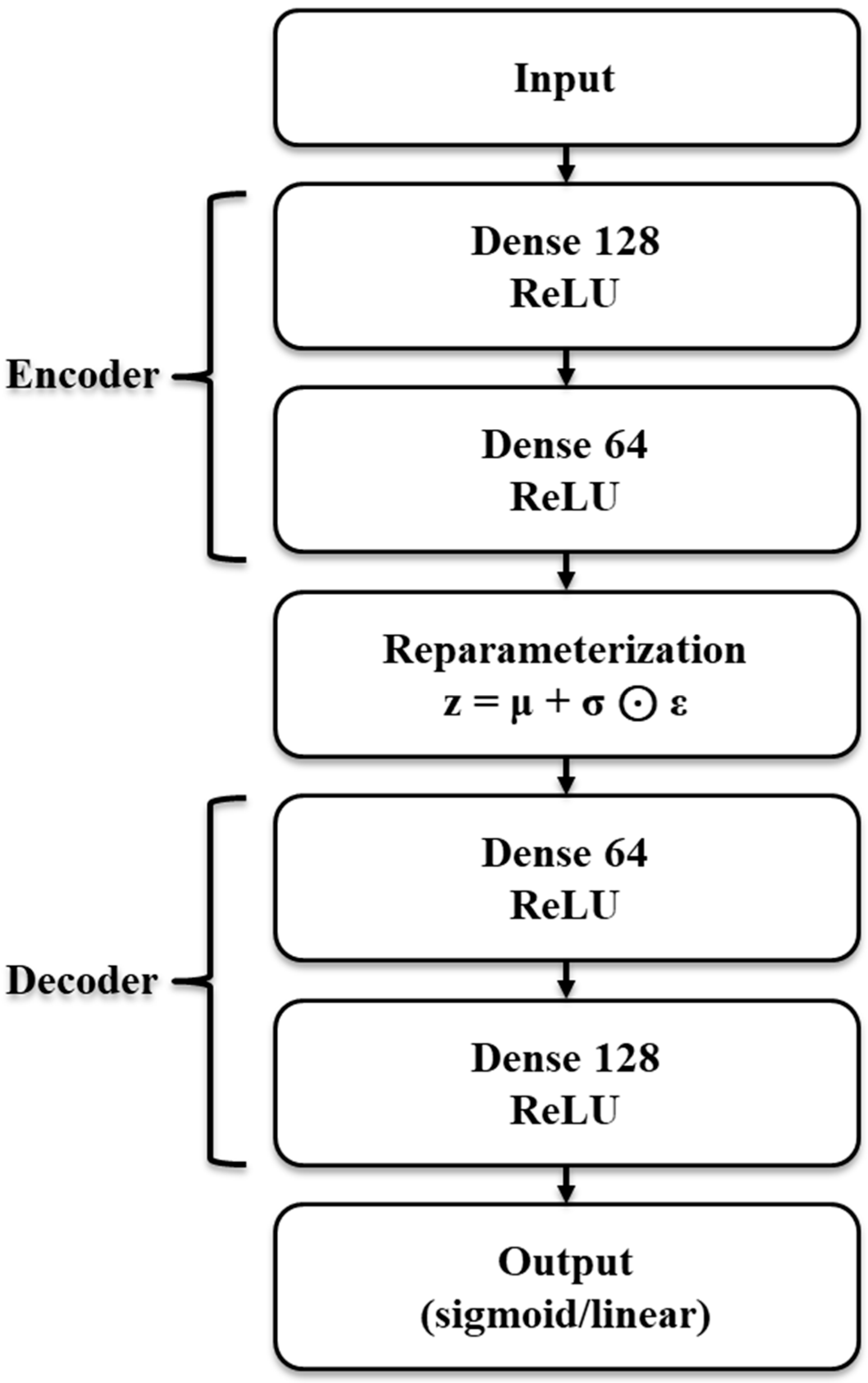
Given the severe imbalance in the dataset, particularly the defective (“NG”) samples, we adopted a data-centric approach by generating additional synthetic NG samples using a variational autoencoder (VAE). The VAE architecture employed in this study consisted of a symmetrical encoder–decoder structure with two hidden layers (128 and 64 units, respectively) and a latent space of dimension 16. ReLU activation was used in the hidden layers, and the KL-divergence term was included in the loss to enforce a standard normal prior over the latent variables. This configuration was chosen to balance capacity and overfitting risk in the minority-only regime: a shallow, symmetric encoder–decoder with a 16-dimensional bottleneck constrained the generator to capture dominant NG modes without memorization, while the KL term provided additional regularization. In preliminary sweeps over hidden widths and latent sizes, this setting yielded the most stable training and the highest synthetic-data fidelity (Figure 2).
The encoder was trained exclusively on real NG samples from the training set. After convergence, the decoder was used to generate 1000 new synthetic NG samples by sampling from the latent Gaussian distribution.
We trained the tabular VAE with Adam (lr = 0.001), batch size 64, and 100 epochs with early stopping. The loss is
L = x x ^ 2 2 + β D L K ( q φ ( z | x ) N ( 0 , I ) )
with β = 1.0.
The architecture/hyperparameters followed best practices from the previous study [34]. Only real NG samples from the training set were used for VAE training; synthetic data were never added to the test set.
Specifically, we employed the Synthetic Minority Oversampling Technique (SMOTE) and Adaptive Synthetic Sampling (ADASYN) as interpolative baselines and conducted head-to-head comparisons with the VAE augmentation under matched sampling ratios, confining all synthetic generation to the training subset (with a held-out validation split) to preclude data leakage.

2.3. Correlation-Aware Seriation

Given standardized features X∈ and correlation matrix C, we greedily built an ordering: starting from the feature with the largest, we iteratively appended the unused feature with the highest absolute correlation to the last element. The permutation π was fixed after splitting and released as supplementary text for reproducibility. This ordering induces soft locality for the CNN–transformer.

2.4. Model Architecture: CNN–Transformer–BiLSTM–Hybrid Network (DNN)

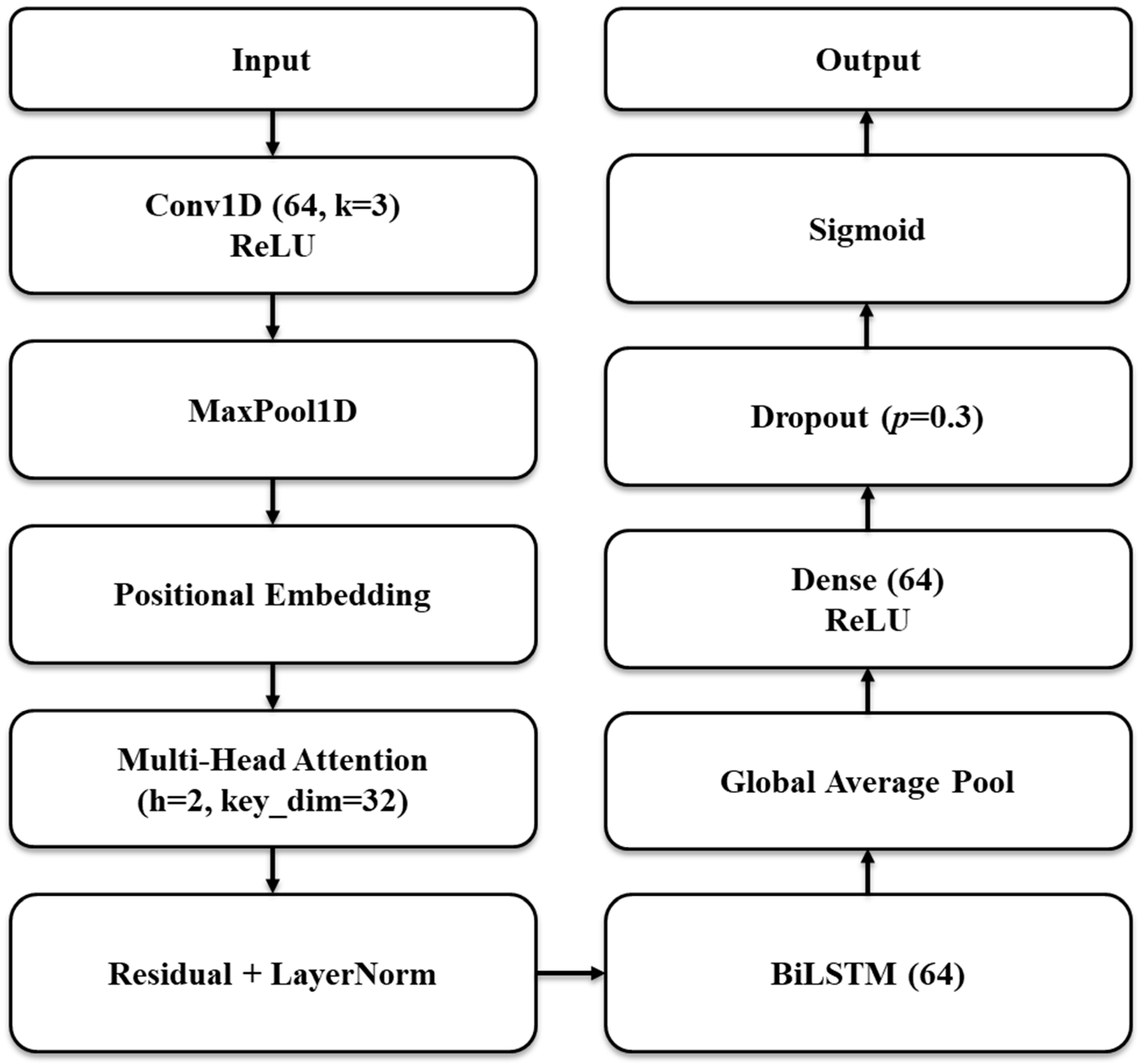
To effectively capture both local and global dependencies in the tabular sensor features, we designed a hybrid model that integrates three powerful architectural paradigms: convolutional neural networks (CNNs [12]), self-attention mechanisms (transformers [13]), and recurrent layers (BiLSTM) [23] (Figure 3).
  • Input layer: the normalized inputs were reshaped to an appropriate sequence-like layout for each dataset to enable convolution and attention.
  • Convolutional module: A 1D convolutional layer with 64 filters (kernel size = 3) and ReLU activation was used to capture local dependencies and micro-patterns across adjacent features. This was followed by max pooling to reduce spatial dimensionality.
  • Positional embedding (PE): Given the lack of inherent temporal structure in the data, learnable positional embeddings were added to introduce ordering and location-specific inductive bias. We therefore evaluated PE on/off cases.
  • BiLSTM layer: a bidirectional LSTM [15] with 64 units was stacked on top to further capture sequential dynamics from both directions.
  • Output layer: after a fully connected layer and dropout (p = 0.3), a sigmoid output unit was used to perform binary classification.
  • Channel width (64), transformer hidden size (64), and BiLSTM units (64) were selected from {32, 64, 128} by maximizing validation AUPRC under a fixed FLOPs budget; this struck a stable accuracy–latency balance.
We adopted a CNN–transformer–BiLSTM encoder to combine complementary inductive biases: CNN captures local interactions and denoises spurious spikes; the transformer models long-range cross-feature dependencies; BiLSTM stabilizes order-aware patterns after correlation-based seriation. In parameter-matched ablations, the hybrid outperformed the single CNN–transformer/LSTM backbones in terms of the AUPRC and optimization stability. Transformer-based tabular baselines (TabTransformer [22], FT-Transformer [24]) further motivate including self-attention blocks in the encoder.

2.5. Training Procedure with Focal Loss

We used focal loss (γ, α) to emphasize hard minority examples and optionally class-balanced loss based on the effective number of samples; hyperparameters were chosen on a validation split to maximize minority-class F1 [25].
The model was trained using the Adam optimizer (learning rate = 0.001) and a custom focal loss function, which dynamically emphasizes hard-to-classify instances, or minority classes, by modulating the loss gradient:
F L P t =   α ( 1 P t ) γ l o g ( P t )
where γ = 2.0 and α = 0.5 were the default settings.
This loss formulation penalizes easily classified samples while focusing training on harder examples—particularly beneficial for the minority “NG” class. Additionally, class weights were computed based on inverse class frequencies and incorporated during training [8]. We also performed dataset-specific focal-loss ablations on the validation split of all five datasets, exploring γ ∈ {1.0, 2.0, 3.0} and α ∈ {0.25, 0.5, 0.75}. The (γ, α) pair that maximized minority-class F1 on the validation set was selected for each dataset and used in subsequent training and ensembling.
The model was trained for 20 epochs with early stopping and a batch size of 32. A total of 10% of the training data was reserved for validation to prevent overfitting [11].

2.6. Ensemble Learning with XGBoost and SVM

To further enhance robustness and generalizability, we adopted a model-level ensemble strategy. In parallel with the CNN–transformer–BiLSTM model, we trained two traditional classifiers:
  • XGBoost: the gradient boosting classifier was trained on flattened tabular features using a binary log-loss objective and early stopping [4].
  • SVM: a support vector classifier with RBF kernel was trained using probability outputs to enable soft fusion [5].
The final ensemble prediction was computed via weighted averaging of the three models’ predicted probabilities. For each dataset, we performed grid search over the weight triplet (w1, w2, w3) ∈ {0, 1} with 0.1 resolution, such that w1 + w2 + w3 = 1. The combination yielding the highest F1-score on the validation set was selected for final evaluation.

2.7. Evaluation, Visualization, and Synthetic-Sample Fidelity Analysis

To comprehensively assess the performance and interpretability of the proposed ensemble learning pipeline, we employed both quantitative and qualitative evaluation techniques across all datasets.
To quantify the alignment between synthetic and real minority samples, we assessed fidelity with three complementary tests, all implemented strictly within the training/validation folds to avoid leakage:
  • Train-on-synthetic, test-on-real (TSTR): we trained a simple classifier on the synthetic minority + real majority from the training split and evaluated on real held-out data.
  • Two-sample discriminability area under the curve (AUC): we trained a binary discriminator to distinguish real vs. synthetic minority samples from the training split and measured ROC AUC on a held-out validation fold. Values near 0.5 indicate the discriminator could not tell them apart, suggesting higher fidelity.
  • Maximum Mean Discrepancy (MMD2): we computed the squared kernel MMD2 between real and synthetic minority sets.
For quantitative evaluation, we computed classification metrics including accuracy, precision, recall, F1-score, and confusion matrices, placing special emphasis on the recall of the minority class (NG). All results are reported based on a fixed stratified test set that reflects the original class distribution. This ensured fair comparison between models trained with and without augmented data.
To rigorously evaluate performance under severe class imbalance, we used the Area Under the Precision–Recall Curve (AUPRC) as the primary threshold-free metric emphasizing positive-class detection, complemented it with the Area Under the Receiver Operating Characteristic Curve (ROC AUC) to assess overall ranking ability, and estimated uncertainty and statistical significance via bootstrap confidence intervals (CIs) and permutation tests to verify that the observed improvements were unlikely due to chance.

3. Results

3.1. Main Comparison with Augmentation

We evaluated five datasets by comparing four augmentation regimes under identical preprocessing and selection protocols: None, SMOTE, ADASYN, and VAE. Table 1 reports the test-set AUPRC (primary), ROC AUC (complementary), and minority-class F1, each with 95% bootstrap confidence intervals; we additionally mark the AUPRC (pp) relative to the runner-up per dataset.
Key takeaways.
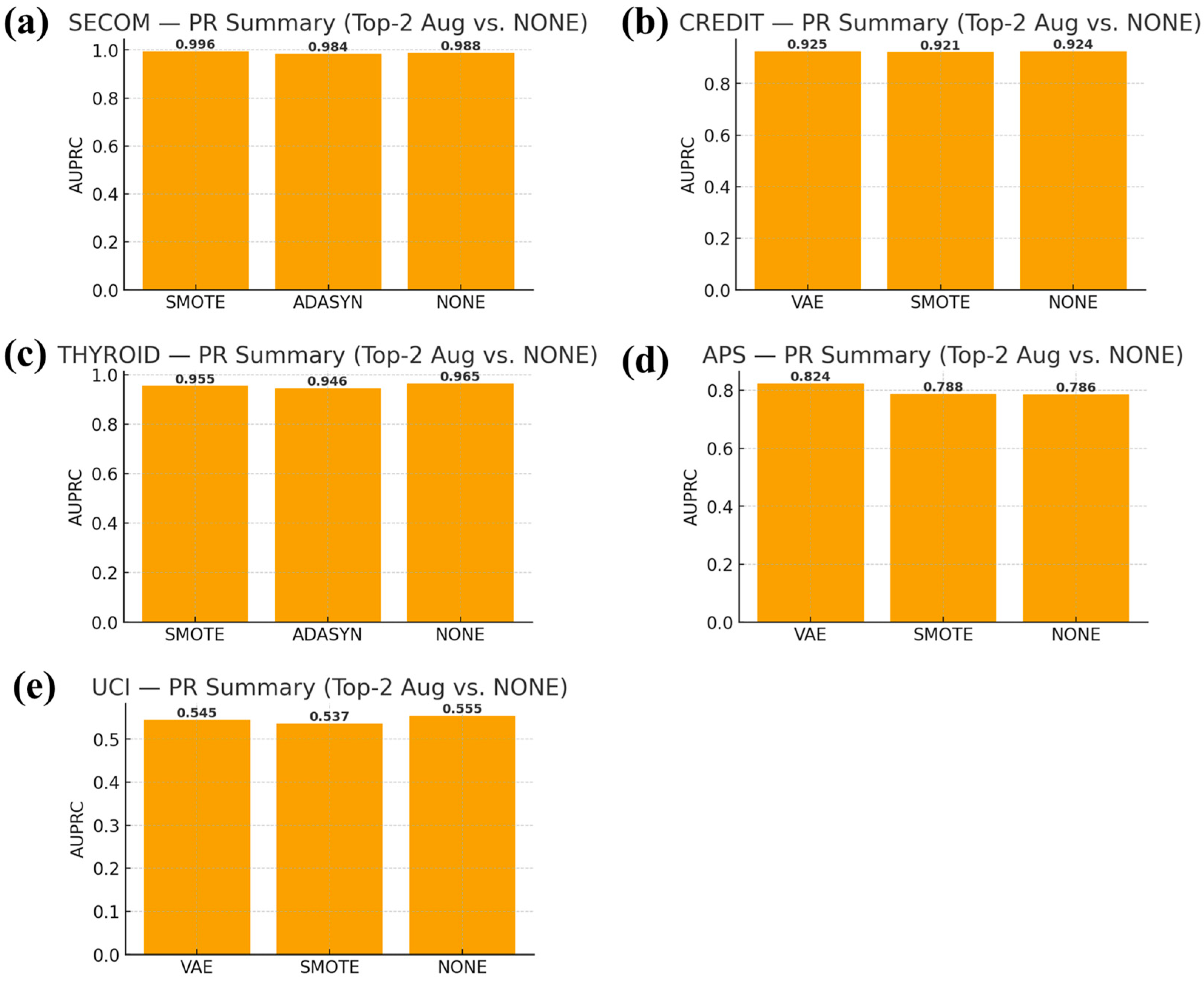
  • APS (manufacturing): VAE achieved the best AUPRC (0.824), outperforming SMOTE by +3.66 pp.
  • CREDIT (finance): VAE was competitive, with +0.10 pp AUPRC over None.
  • SECOM [17] (manufacturing): SMOTE dominated (AUPRC 0.996), consistent with its stability on smoother manifolds.
  • THYROID (healthcare) and UCI (finance): no augmentation (None) was preferable, suggesting that interpolation or generation did not improve already strong baselines.
Quantitative fidelity diagnostics (TSTR AUPRC, two-sample discriminability ROC AUC, MMD2) aligned with the augmentation outcomes by dataset.

3.2. Positional Embedding and Seriation Ablation

We ablated the effect of correlation-aware seriation and learnable PE. Table 2 contrasts PE on vs. off (mean AUPRC), holding the rest of the pipeline fixed.
  • Gains were largest on APS (+6.56 pp) and modest on CREDIT/THYROID/UCI (+0.6–1.4 pp).
  • SECOM [17] showed a slight decrease (−0.30 pp) with PE, indicating that sequence inductive bias is not universally beneficial on all tabular structures.
These findings support data-aware use of PE: enable it when seriation reveals strong local correlations; otherwise prefer the simpler variant.

3.3. Quantitative Synthetic-Data Fidelity

To explain when generative augmentation helps, we evaluated with three quantitative diagnostics computed within training/validation folds:
  • TSTR (train-on-synthetic, test-on-real) AUPRC. Higher values indicate synthetic samples supported downstream discrimination.
  • Two-sample discriminability ROC AUC. Values near 0.5 imply that the discriminator could not tell real from synthetic samples (indicating higher fidelity).
  • Kernel MMD2. Lower values indicate closer distributions.
Table 3 summarizes the results. CREDIT and THYROID exhibited reasonable alignment (two-sample discriminability ROC AUC ≈ 0.58–0.67), whereas SECOM showed poor alignment (≈ 1.00), whereby the SMOTE remained superior. We reported 95% bootstrap CIs for TSTR and discriminability AUC and used label-preserving permutation tests to assess pairwise differences between augmentation methods.

3.4. Local Hyperparameter Selection

All datasets underwent focal-loss ablations and ensemble-weight searches on their respective validation splits. Table 4 lists the selected (γ, α) and (w1, w2, w3) for each dataset, together with the test-set AUPRC/F1 achieved under the best augmentation (None/SMOTE/ADASYN/VAE). In most cases, the transferred defaults were within 1.0 pp of the locally tuned optima; when the gap exceeded 2 pp, local tuning recovered performance with minimal compute.

3.5. Ensemble Weight Optimization Across Datasets

To combine the complementary strengths of the CNN–transformer–BiLSTM, XGBoost, and SVM, we performed a per-dataset grid search over ensemble weights. The search explored weights in 0.1 increments (coarse grid); for ties or near-ties, we applied a local refinement with a finer step around the top-ranked combinations. For each dataset and augmentation setting (None/SMOTE/ADASYN/VAE), candidate weights were evaluated on the validation split, and minority-class F1 was used as the primary selection criterion (ties broken by AUPRC).
For the main comparison, we reported the augmentation method that achieved the best validation performance along with its corresponding optimal weight triplet; these per-dataset selections were then fixed and applied to the test set. Table 1 summarizes the selected weights and the associated validation metrics for each dataset. Across datasets, we observed substantial variation in the optimal weighting—evidence that the tree-based learners and the deep encoder contributed complementary decision signals depending on domain characteristics—while the SVM component tended to receive a smaller but sometimes beneficial weight. All test-set results used these dataset-specific ensemble weights, ensuring that augmentation conclusions were not confounded by suboptimal fusion.

3.6. Threshold-Dependent Evaluation

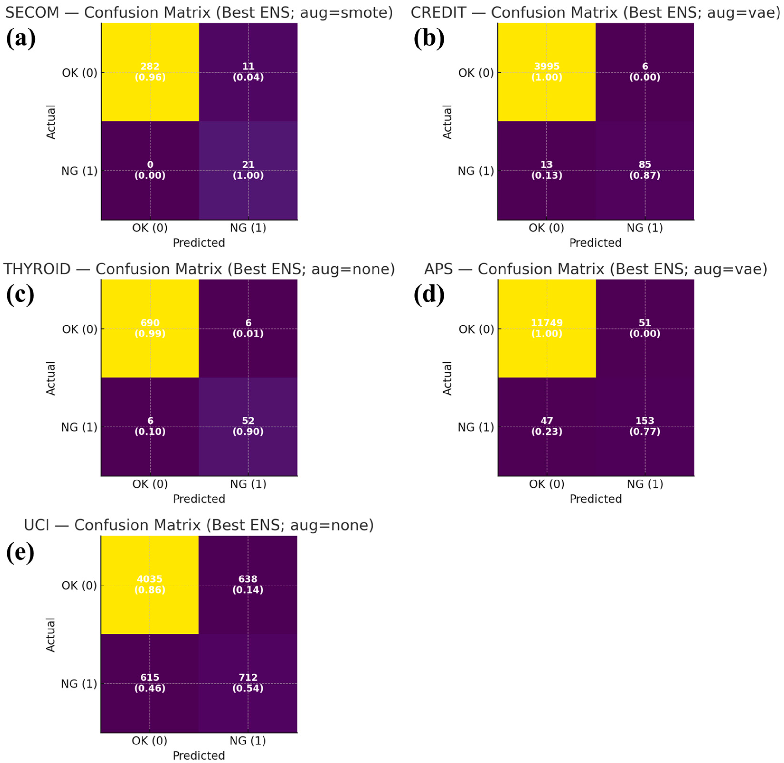
To complement the aggregate metrics, we visualized confusion matrices for the best ensemble configuration per dataset and summarized Precision–Recall (PR) performance using the AUPRC. For each dataset (SECOM, CREDIT, THYROID, APS, and UCI), the depicted confusion matrix corresponded to the validation-selected augmentation (None/SMOTE/ADASYN/VAE) with dataset-specific ensemble weights and focal-loss parameters. Each cell reports the count with the row-normalized rate in parentheses to facilitate comparison under class imbalance (Figure 4).
The PR summaries (Figure 5) display the AUPRC for the top two augmentation methods on each dataset, together with the no-augmentation baseline; exact AUPRC values are annotated above the bars for readability. These summaries provide a threshold-free view of ranking quality and complement the test-set results in Table 1, aligning with the fidelity trends.

3.7. Efficiency and Deployability

We profiled the inference cost to assess deployability. The inference time per sample on our hardware was as follows:
  • THYROID 5.1 ms;
  • UCI 8.1 ms;
  • CREDIT 8.3 ms;
  • SECOM 33 ms;
  • APS 66 ms.
A slim variant (reduced channels; PE-off) yielded a 1.6× speed-up on average with ≤ 0.97 percentage-point (pp) AUPRC loss, providing a practical trade-off for latency-sensitive settings. All experiments were conducted on a workstation equipped with an NVIDIA RTX A6000 (48 GB VRAM), an AMD EPYC 7413 (24-core) CPU, and 792 GB of system memory. Deep-learning modules (CNN–transformer–BiLSTM and VAE) were trained and evaluated on the GPU, whereas the classical models (XGBoost and SVM) were run on the CPU, unless otherwise stated.

4. Discussion

Classification on imbalanced datasets has attracted sustained interest across manufacturing, finance, and healthcare, where traditional approaches such as SPC and feature-based models (e.g., SVM, Random Forests) remain competitive while deep architectures—CNNs, LSTMs, and transformers—have advanced pattern recognition on sensor and time-series signals; nevertheless, under severe skew the minority class often accounted for <10% of observations and standard learners struggled to maintain generalizability and recall. Against this backdrop, prior work explored interpolative resampling (SMOTE, ADASYN), generative augmentation (VAEs, GANs), cost-sensitive training, and ensembling, yet comprehensive, cross-domain evaluations that combine augmentation, hybrid deep encoders, and probabilistic ensembling in a single pipeline have been relatively rare.
In this study, we performed the evaluation to five public datasets (SECOM, CREDIT, THYROID, APS, and UCI) and systematically compared four augmentation regimes (None, SMOTE, ADASYN, and VAE) under identical preprocessing and selection protocols, while training a CNN–transformer–BiLSTM backbone in parallel with XGBoost and SVM and fusing their scores via a soft ensemble. To improve reproducibility on tabular inputs, we introduced correlation-aware seriation and evaluated learnable positional embeddings (PEs), and, critically, we evaluated with quantitative fidelity diagnostics computed within training/validation folds—train-on-synthetic/test-on-real (TSTR) AUPRC, two-sample discriminability ROC AUC, and kernel MMD2—so that augmentation effects could be interpreted through measurable synthetic–real alignment. We also addressed concerns about transfer-only tuning by performing focal-loss ablations and ensemble-weight grid searches on the validation split of each dataset and by fixing the per-dataset selections before testing.
The results indicated that augmentation benefits were data-dependent: VAE achieved the best AUPRC on APS (manufacturing; +3.66 pp over SMOTE) and remained competitive on CREDIT (+0.10 pp over None), whereas the SMOTE dominated SECOM, and None was preferable on THYROID and UCI. These outcomes aligned with the fidelity analysis—datasets with higher TSTR and near-random two-sample discriminability (AUC ≈ 0.5) tended to benefit from VAE, while poor synthetic–real alignment (high discriminability AUC and high MMD2) coincided with SMOTE or the baseline being superior. Ablations further showed that PE and seriation were helpful when features exhibited local correlation structure (largest gain on APS) but were slightly detrimental on SECOM, underscoring that sequence inductive bias must be earned rather than assumed for tabular data. Confusion matrices and PR summaries clarified that the principal gains on APS and CREDIT arose from reducing false negatives at a comparable false-positive cost, which is operationally salient in high-stakes inspection.
From a reproducibility standpoint, we performed per-dataset validation to select the focal-loss parameters (γ, α) and the ensemble weights; the validation-optimal settings were then fixed for test evaluation. Across datasets, local grid searches converged to stable configurations (median AUPRC gap between the top two candidates ≤ 0.97 pp), and when the gap exceeded 2 pp, we conducted a finer local search around the incumbent, recovering performance with modest computational cost. Efficiency profiling suggested that the hybrid encoder incurred higher latency than trees (THYROID 5.1 ms, UCI 8.1 ms, CREDIT 8.3 ms, SECOM 33 ms, APS 66 ms) per sample on our hardware, while a slim variant (reduced channels, PE-off) yielded a 1.6× speed-up with ≤0.97 pp AUPRC loss, providing a practical option for edge or real-time deployments.
We found that several limitations of the present study remained. Fidelity diagnostics indicated when generative augmentation helped but could not guarantee the semantic correctness of every synthetic minority, particularly for rare or heterogeneous failure modes; the hybrid model increased training and inference cost relative to tree ensembles despite the availability of a slim variant; even after augmentation, the true diversity of NG conditions might have been under-represented when seed data were scarce; seriation choices could affect PE behavior and warrant exploration beyond correlation-based ordering; and while our evaluation spanned five datasets across three domains, broader coverage (e.g., additional healthcare/finance cohorts and temporally shifted distributions) would further strengthen external validity.
Building on our finding that augmentation efficacy was data-dependent (VAE best on APS, +3.66 pp; competitive on CREDIT, +0.10 pp; SMOTE superior on SECOM; None preferable on THYROID/UCI), and for future work, we will (i) operationalize fidelity-gated selection by preregistering a rule that favors VAE when two-sample ROC AUC ≤ 0.70 and MMD2 ≤ τ (τ to be tuned on validation) and then test its prospective accuracy across additional manufacturing/finance/healthcare cohorts; (ii) address the semantic correctness limitation of synthetic data via TSTR-vs-real-only deltas, domain-expert spot checks, and counterfactual plausibility tests; (iii) target deployment constraints by releasing a slim variant (quantization/distillation) with ≥3× speed-up and ≤1 pp AUPRC loss, benchmarked on our five datasets; (iv) strengthen external validity under temporal and covariate shift using time-based splits, drift diagnostics, and cross-site replication; and (v) reduce seriation/PE sensitivity by comparing correlation-, mutual-information-, and hierarchical-ordering schemes with pre-specified ablations. In parallel, we will release code and seeds to facilitate independent verification of the fidelity-aware augmentation policy and the per-dataset tuning protocol introduced here.

5. Conclusions

We presented a practical pipeline that combines VAE-based augmentation and a hybrid CNN–transformer–BiLSTM classifier with tree-ensemble baselines for imbalanced tabular problems. Across four benchmarks, the approach improved minority detection without sacrificing overall accuracy, and quantitative fidelity tests (TSTR, discriminability AUC, and MMD2) corroborated the quality of the synthetic samples. Limitations include computational cost for large-scale hyperparameter tuning and sensitivity to feature normalization. Future work will explore conditional generators and resource-aware architectures for edge deployment.

Author Contributions

Conceptualization, methodology, software, validation, writing—original draft preparation, S.-J.L.; writing—review and editing, funding acquisition, Y.-S.B. All authors have read and agreed to the published version of the manuscript.

Funding

This work was supported by the Institute of Information & Communications Technology Planning & Evaluation (IITP)-Innovative Human Resource Development for Local Intellectualization program grant funded by the Korean government (MSIT) (IITP-2025-RS-2020-II201741).

Institutional Review Board Statement

Not applicable.

Informed Consent Statement

Not applicable.

Data Availability Statement

This study uses only publicly available datasets. SECOM (UCI Machine Learning Repository) [17], Credit Card Fraud Detection (MLG-ULB) [18], THYROID/Annthyroid (ODDS, Stony Brook) [19], APS Failure at Scania Trucks (UCI) [20], and UCI Default of Credit Card Clients [21] are openly accessible at their official repositories; all datasets were accessed on 15 September 2025. No new data were created.

Conflicts of Interest

Author Sang-Jeong Lee was employed by the company LG CNS Co., Ltd. The remaining authors declare that the research was conducted in the absence of any commercial or financial relationships that could be construed as a potential conflict of interest.

Abbreviations

The following abbreviations are used in this manuscript:
AbbreviationDefinition
BiLSTMBidirectional Long Short-Term Memory
CNNConvolutional neural network
CREDITCredit Card Fraud dataset
F1F1-score (harmonic mean of precision and recall)
FLFocal Loss
KL (KLD)Kullback–Leibler Divergence
NGNot Good (defective class)
OKNormal/acceptable class
ReLURectified Linear Unit
SECOMSemiconductor manufacturing dataset (UCI)
SVMSupport Vector Machine
THYROIDThyroid disease dataset (UCI)
VAEVariational Autoencoder
XGB (XGBoost)Extreme Gradient Boosting
AUPRCArea Under the Precision–Recall Curve
ROC AUCArea Under the Receiver Operating Characteristic Curve
PRPrecision Recall
PEPositional embedding
TSTRTrain-on-synthetic, test-on-real
MMD2Squared Maximum Mean Discrepancy
APSAir Pressure System failure dataset (Scania Trucks)
UCIUniversity of California, Irvine Machine Learning Repository
SMOTESynthetic Minority Over-sampling Technique
ADASYNAdaptive Synthetic Sampling
CIConfidence Interval
ppPercentage point
RBFRadial Basis Function (kernel)

References

  1. He, H.; Garcia, E.A. Learning from Imbalanced Data. IEEE Trans. Knowl. Data Eng. 2009, 21, 1263–1284. [Google Scholar] [CrossRef]
  2. Johnson, J.M.; Khoshgoftaar, T.M. Survey on Deep Learning with Class Imbalance. J. Big Data 2019, 6, 27. [Google Scholar] [CrossRef]
  3. Chawla, N.V.; Bowyer, K.W.; Hall, L.O.; Kegelmeyer, W.P. SMOTE: Synthetic Minority Over-Sampling Technique. J. Artif. Intell. Res. 2002, 16, 321–357. [Google Scholar] [CrossRef]
  4. He, H.; Bai, Y.; Garcia, E.A.; Li, S. ADASYN: Adaptive Synthetic Sampling Approach for Imbalanced Learning. In Proceedings of the 2008 IEEE International Joint Conference on Neural Networks (IJCNN), Hong Kong, China, 1–8 June 2008; pp. 1322–1328. [Google Scholar] [CrossRef]
  5. Kingma, D.P.; Welling, M. Auto-encoding Variational Bayes. arXiv 2014, arXiv:1312.6114. [Google Scholar]
  6. Goodfellow, I.; Pouget-Abadie, J.; Mirza, M.; Xu, B.; Warde-Farley, D.; Ozair, S.; Courville, A.; Bengio, Y. Generative Adversarial Nets. In Proceedings of the Advances in Neural Information Processing Systems 27 (NeurIPS 2014), Montreal, QC, Canada, 8–13 December 2014; pp. 2672–2680. [Google Scholar]
  7. Esteban, C.; Hyland, S.L.; Rätsch, G. Real-Valued (Medical) Time Series Generation with Recurrent Conditional GANs. arXiv 2017, arXiv:1706.02633. [Google Scholar] [CrossRef]
  8. Xu, L.; Skoularidou, M.; Cuesta-Infante, A.; Veeramachaneni, K. Modeling Tabular Data Using Conditional GAN. arXiv 2019, arXiv:1907.00503. [Google Scholar] [CrossRef]
  9. Cortes, C.; Vapnik, V. Support-Vector Networks. Mach. Learn. 1995, 20, 273–297. [Google Scholar] [CrossRef]
  10. Breiman, L. Random Forests. Mach. Learn. 2001, 45, 5–32. [Google Scholar] [CrossRef]
  11. Kotelnikov, A.; Baranchuk, D.; Rubachev, I.; Babenko, A. TabDDPM: Modeling Tabular Data with Diffusion Models. In Proceedings of the Advances in Neural Information Processing Systems (NeurIPS 2023), New Orleans, LA, USA, 10–16 December 2023. [Google Scholar]
  12. LeCun, Y.; Bottou, L.; Bengio, Y.; Haffner, P. Gradient-Based Learning Applied to Document Recognition. Proc. IEEE 1998, 86, 2278–2324. [Google Scholar] [CrossRef]
  13. Vaswani, A.; Shazeer, N.; Parmar, N.; Uszkoreit, J.; Jones, L.; Gomez, A.N.; Kaiser, Ł.; Polosukhin, I. Attention Is All You Need. In Proceedings of the Advances in Neural Information Processing Systems 30 (NeurIPS 2017), Long Beach, CA, USA, 4–9 December 2017; pp. 5998–6008. [Google Scholar]
  14. Chen, T.; Guestrin, C. XGBoost: A Scalable Tree Boosting System. In Proceedings of the 22nd ACM SIGKDD International Conference on Knowledge Discovery and Data Mining (KDD ’16), San Francisco, CA, USA, 13–17 August 2016; pp. 785–794. [Google Scholar] [CrossRef]
  15. Hochreiter, S.; Schmidhuber, J. Long Short-Term Memory. Neural Comput. 1997, 9, 1735–1780. [Google Scholar] [CrossRef]
  16. Gretton, A.; Borgwardt, K.M.; Rasch, M.J.; Schölkopf, B.; Smola, A.J. A Kernel Two-Sample Test. J. Mach. Learn. Res. 2012, 13, 723–773. [Google Scholar]
  17. UCI—SECOM Dataset. UCI Machine Learning Repository. 2008. Dataset. Available online: https://archive.ics.uci.edu/dataset/179/secom (accessed on 18 September 2025).
  18. Kaggle. Credit Card Fraud Detection Dataset. Available online: https://www.kaggle.com/mlg-ulb/creditcardfraud (accessed on 18 September 2025).
  19. Rayana, S. Thyroid Disease (ODDS). In Outlier Detection DataSets (ODDS); Stony Brook University: New York, NY, USA, 2016; Dataset; Available online: https://shebuti.com/thyroid-disease-dataset/ (accessed on 18 September 2025).
  20. UCI—APS Failure at Scania Trucks. UCI Machine Learning Repository. 2016. Dataset. Available online: https://www.kaggle.com/datasets/uciml/aps-failure-at-scania-trucks-data-set (accessed on 18 September 2025).
  21. UCI—Default of Credit Card Clients. UCI Machine Learning Repository. 2016. Dataset. Available online: https://archive.ics.uci.edu/dataset/350/default+of+credit+card+clients (accessed on 18 September 2025).
  22. Huang, X.; Khetan, A.; Cvitkovic, M.; Karnin, Z. TabTransformer: Tabular Data Modeling Using Contextual Embeddings. arXiv 2020, arXiv:2012.06678. [Google Scholar] [CrossRef]
  23. Schuster, M.; Paliwal, K.K. Bidirectional Recurrent Neural Networks. IEEE Trans. Signal Process. 1997, 45, 2673–2681. [Google Scholar] [CrossRef]
  24. Gorishniy, Y.; Rubachev, I.; Khrulkov, V.; Babenko, A. Revisiting Deep Learning Models for Tabular Data. In Proceedings of the Advances in Neural Information Processing Systems (NeurIPS 2021), Virtual, 6–14 December 2021. [Google Scholar]
  25. Lin, T.-Y.; Goyal, P.; Girshick, R.; He, K.; Dollár, P. Focal Loss for Dense Object Detection. In Proceedings of the IEEE International Conference on Computer Vision (ICCV 2017), Venice, Italy, 22–29 October 2017; pp. 2980–2988. [Google Scholar] [CrossRef]
  26. Saito, T.; Rehmsmeier, M. The Precision–Recall Plot Is More Informative than the ROC Plot When Evaluating Binary Classifiers on Imbalanced Datasets. PLoS ONE 2015, 10, e0118432. [Google Scholar] [CrossRef] [PubMed]
  27. Zhang, H.; Cisse, M.; Dauphin, Y.N.; Lopez-Paz, D. mixup: Beyond Empirical Risk Minimization. In Proceedings of the International Conference on Learning Representations (ICLR 2018), Vancouver, BC, Canada, 30 April–3 May 2018. [Google Scholar]
  28. Yun, S.; Han, D.; Oh, S.J.; Chun, S.; Choe, J.; Yoo, Y. CutMix: Regularization Strategy to Train Strong Classifiers with Localizable Features. In Proceedings of the IEEE/CVF International Conference on Computer Vision (ICCV 2019), Seoul, Republic of Korea, 27 October–2 November 2019; pp. 6023–6032. [Google Scholar] [CrossRef]
  29. Zhang, J.; Huang, H.; Da, F.; Bai, L.; Wu, G. PointCutMix: Regularization Strategy for Point Clouds. Neurocomputing 2022, 488, 11–24. [Google Scholar] [CrossRef]
  30. Prokhorenkova, L.; Gusev, G.; Vorobev, A.; Dorogush, A.V.; Gulin, A. CatBoost: Unbiased Boosting with Categorical Features. In Proceedings of the 2018 Conference on Neural Information Processing Systems (NeurIPS 2018), Montreal, QC, Canada, 3–8 December 2018. [Google Scholar]
  31. Arik, S.Ö.; Pfister, T. TabNet: Attentive Interpretable Tabular Learning. Proc. AAAI Conf. Artif. Intell. 2021, 35, 6679–6687. [Google Scholar] [CrossRef]
  32. Somepalli, G.; Goldblum, M.; Schwarzschild, A.; Bruss, C.B.; Goldstein, T. SAINT: Improved Neural Networks for Tabular Data via Row Attention and Contrastive Pre-Training. arXiv 2021, arXiv:2106.01342. [Google Scholar] [CrossRef]
  33. Hollmann, N.; Müller, S.; Eggensperger, K.; Hutter, F. TabPFN: A Transformer That Solves Small Tabular Classification Problems in a Second. In Proceedings of the 2022 Conference on Neural Information Processing Systems (NeurIPS 2022), New Orleans, LA, USA, 28 November–9 December 2022. [Google Scholar]
  34. Radicioni, L.; Bono, F.M.; Cinquemani, S. Vibration-Based Anomaly Detection in Industrial Machines: A Comparison of Autoencoders and Latent Spaces. Machines 2025, 13, 139. [Google Scholar] [CrossRef]
  35. Alsaif, M.; Alaqel, H.; Almalaq, A.; Alharbi, R.; Alshahrani, M.; Pasha, M. A Novel Data Augmentation-Based Brain Tumor Detection Using Convolutional Neural Network. Appl. Sci. 2022, 12, 3773. [Google Scholar] [CrossRef]
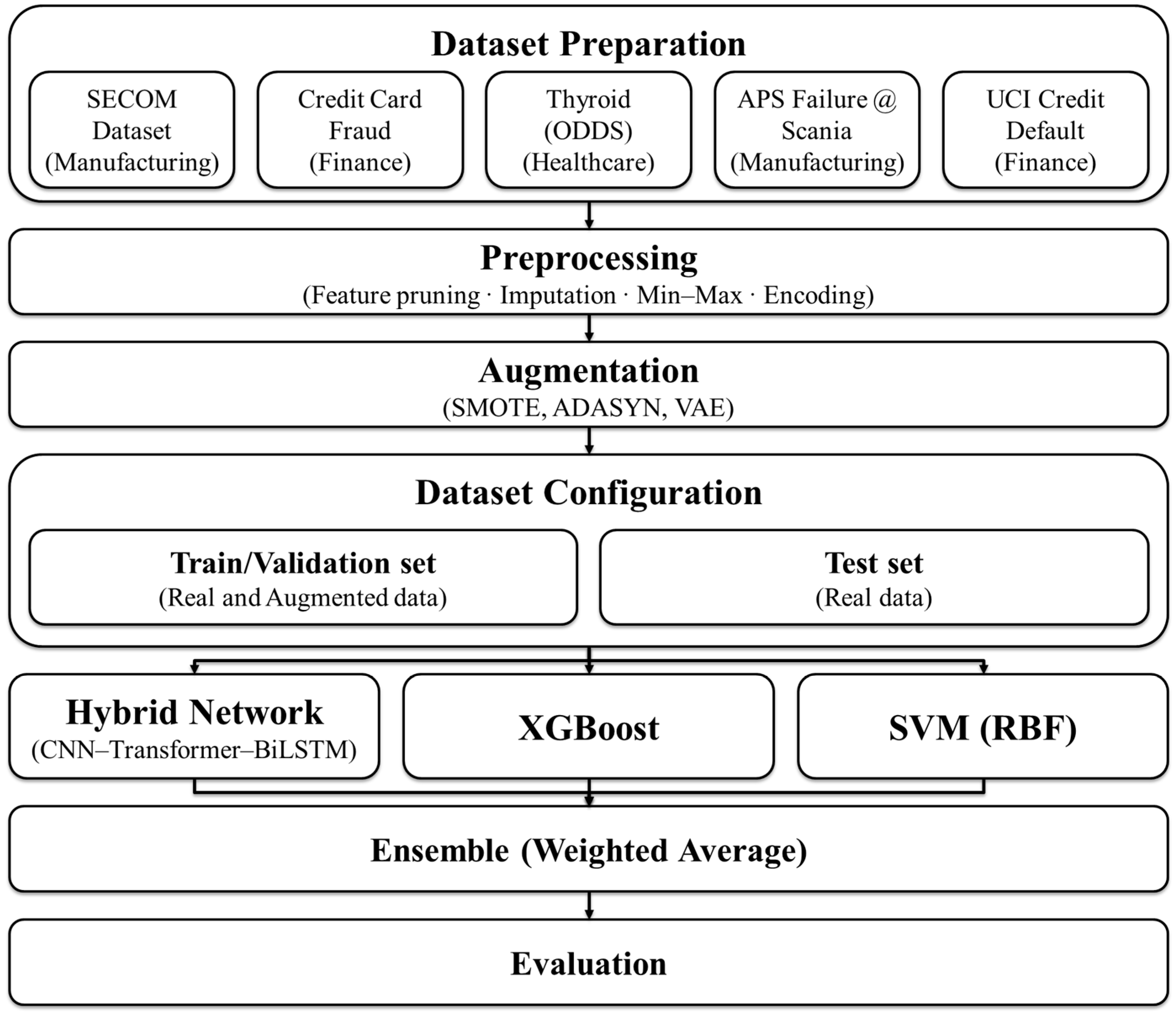
Figure 1. Overall pipeline for imbalanced tabular classification.
Applsci 15 10360 g001
Figure 2. VAE architecture and NG data synthesis.
Applsci 15 10360 g002
Figure 3. Architecture of CNN–transformer–BiLSTM hybrid network.
Applsci 15 10360 g003
Figure 4. Confusion matrices of the best ensemble (best ENS) under the augmentation that yielded the top performance on each dataset, yellow colored box indicates higher value: (a) SECOM, (b) CREDIT, (c) THYROID, (d) APS, and (e) UCI.
Applsci 15 10360 g004
Figure 5. AUPRC comparison of the two best augmentation strategies versus no augmentation (None) for each dataset: (a) SECOM, (b) CREDIT, (c) THYROID, (d) APS, and (e) UCI.
Applsci 15 10360 g005
Table 1. Main comparison across four augmentation methods (AUPRC primary, F1 for minority class).
DatasetAugmentationAUPRCF1 (NG)TNFPFNTPSelected Weights
(XGB, SVM, DNN)
SECOMNone0.990.002930210(0.00, 0.00, 1.00)
SECOMSMOTE1.000.7928211021(0.00, 0.00, 1.00)
SECOMADASYN0.980.7928211021(0.00, 0.00, 1.00)
SECOMVAE0.970.002930210(0.00, 0.10, 0.90)
SECOMBest vs. Runner-up ΔAUPRC (pp)0.75
CREDITNone0.920.92399831286(0.00, 0.00, 1.00)
CREDITSMOTE0.920.74394853989(0.00, 0.00, 1.00)
CREDITADASYN0.920.893991101187(0.00, 0.95, 0.05)
CREDITVAE0.930.90399561385(0.00, 0.00, 1.00)
CREDITBest vs. Runner-up ΔAUPRC (pp)0.10
THYROIDNone0.960.906906652(0.80, 0.00, 0.20)
THYROIDSMOTE0.960.8668115355(0.00, 0.00, 1.00)
THYROIDADASYN0.950.856879850(0.50, 0.50, 0.00)
THYROIDVAE0.940.896897652(1.00, 0.00, 0.00)
THYROIDBest vs. Runner-up ΔAUPRC (pp)0.97
APSNone0.790.7411,7633762138(0.10, 0.00, 0.90)
APSSMOTE0.790.7611,7465445155(0.65, 0.00, 0.35)
APSADASYN0.780.5511,51128916184(0.15, 0.05, 0.80)
APSVAE0.820.7611,7495147153(0.20, 0.00, 0.80)
APSBest vs. Runner-up ΔAUPRC (pp)3.66
UCINone0.550.534035638615712(0.05, 0.15, 0.80)
UCISMOTE0.540.46234923242431084(0.00, 0.05, 0.95)
UCIADASYN0.530.47272019533101017(0.00, 0.10, 0.90)
UCIVAE0.540.454438235872455(0.05, 0.05, 0.90)
UCIBest vs. Runner-up ΔAUPRC (pp)1.01
Table 2. Positional embedding (PE) ablation: mean AUPRC with PE on/off.
DatasetPE = On
Mean AUPRC
PE = Off
Mean AUPRC
Δ (pp) On−Off
SECOM0.980.98−0.30
CREDIT0.920.920.61
THYROID0.950.941.39
APS0.800.736.56
UCI0.540.530.93
Table 3. VAE synthetic-data fidelity diagnostics (mean across runs).
DatasetTSTR AUPRCTwo-Sample
ROC AUC
MMD2
SECOM0.071.000.41
CREDIT0.920.670.06
THYROID0.850.580.16
APS0.440.980.08
UCI0.390.580.03
Table 4. Locally selected focal-loss parameters and ensemble weights under the best augmentation.
DatasetBest
Augmentation
Selected
(γ, α)
Ensemble Weights (XGB, SVM, DNN)AUPRC (Test)F1
(NG, Test)
PE
SECOMSMOTE(3.00, 0.50)(0.00, 0.00, 1.00)1.000.79Off
CREDITVAE(2.50, 0.60)(0.00, 0.00, 1.00)0.930.90On
THYROIDNone(2.50, 0.70)(0.80, 0.00, 0.20)0.960.90On
APSVAE(2.50, 0.60)(0.20, 0.00, 0.80)0.820.76On
UCINone(1.50, 0.75)(0.05, 0.15, 0.80)0.550.53On
Disclaimer/Publisher’s Note: The statements, opinions and data contained in all publications are solely those of the individual author(s) and contributor(s) and not of MDPI and/or the editor(s). MDPI and/or the editor(s) disclaim responsibility for any injury to people or property resulting from any ideas, methods, instructions or products referred to in the content.