Article

Validity Evaluation of Wind Turbine Monitoring Data by Correlative Coupling Relationship

1
School Energy and Mechanical Engineering, Shanghai University of Electric Power, Shanghai 200090, China
2
Shanghai Key Laboratory of Materials Protection and Advanced Materials in Electric Power, Shanghai 200090, China
3
Shanghai Non-Carbon Energy Conversion and Utilization Institute, Shanghai 200240, China
4
Engineering Research Center of Offshore Wind Technology Ministry of Education, Shanghai University of Electric Power, Shanghai 200090, China
*
Authors to whom correspondence should be addressed.
Appl. Sci. 2025, 15(19), 10320; https://doi.org/10.3390/app151910320
Submission received: 22 August 2025 / Revised: 18 September 2025 / Accepted: 19 September 2025 / Published: 23 September 2025

Abstract

In addressing the potential anomalies in wind turbine monitoring data, it is essential to note that a single data source cannot independently ascertain the validity of data. This paper proposes a correlation coupling judgment algorithm designed to evaluate the validity of wind turbine monitoring data. By quantitatively analyzing the degree of correlation between various sensor data using the Pearson correlation coefficient, this study reveals that data characteristics significantly influence the correlation coefficient. The analysis also examines the effects of filtering, signal phase differences, and interference signals on correlation. The results indicate that effective data preprocessing, can dramatically enhance correlation, while phase shifts and noise interference significantly degrade it. Identifying and mitigating these interfering signals is thus established as a crucial prerequisite for defining reliable correlation criteria. Therefore, this study demonstrates that effective data preprocessing is a necessary step for any correlation-based validity assessment framework.

1. Introduction

In the macro context of global efforts to address climate change and energy transition, the shift from traditional fossil fuel dominance to renewable energy has become inevitable [1,2,3,4]. Wind power has emerged as a significant force in the renewable energy sector due to its abundant resources and environmental friendliness [5,6]. Currently, the installed capacity of wind power is experiencing rapid growth worldwide, and large-scale wind turbines are continuously deployed. Hence, their role in the energy supply system is becoming increasingly prominent [7,8]. However, the operating environment of wind turbines is extremely complex [9] since the interaction of various meteorological factors together with their own mechanical and electrical characteristics are closely coupled [10]. External conditions, such as the intermittency of wind speed, variability of wind direction, and fluctuations in temperature and pressure, can lead to dynamic variations in the operating parameters of wind turbines, including output power, rotational speed, and blade stress. To ensure the efficient and stable operation of wind turbines, it is essential to conduct real-time monitoring of their operational status and evaluate the validity of the data to promptly implement effective maintenance and management measures [9,11]. Therein, in-depth analysis of the monitoring data can detect the underlying patterns and characteristics, which can provide robust support for the optimized operation, fault diagnosis, and performance evaluation of wind turbines [12].
Due to the potential anomalies that may arise during data collection, a single data source cannot independently determine the validity of the data. However, inherent logical relationships often exist among various parameters. Consequently, the validity of data can be assessed based on other parameters that exhibit strong correlations with them [13]. Obviously, an appropriate correlation analysis method is crucial for evaluating the validation of wind turbine monitoring data. However, traditional methods exhibit certain limitations when addressing multivariate data with complex correlation relationships. Currently, mainstream correlation analysis methods include Spearman’s rank correlation analysis, gray relational analysis, and Pearson correlation analysis, among others. Notably, Spearman’s rank correlation analysis is not constrained by the distribution of variables and is well suited for non-normally distributed data, effectively addressing non-linear monotonic relationships [14]. Gray relational analysis requires a limited amount of data and is particularly suitable for scenarios with insufficient data and ambiguous information [15]. While the aforementioned methods offer valuable insights, their application to wind turbine monitoring data presents specific challenges. Spearman’s rank correlation analysis, though robust to non-normality, may overlook precise linear relationships critical for operational parameters [16]. Gray relational analysis introduces subjectivity in parameter selection, which is undesirable for automated, real-time validity assessment systems required in wind farm operations [17]. The operating parameters of wind turbines often exhibit strong linear or approximately linear correlations under stable conditions. This inherent characteristic makes the Pearson correlation coefficient, with its computational efficiency and precise quantification of linear relationships, a highly suitable candidate [18,19]. However, direct application of Pearson correlation is susceptible to data quality issues such as noise and phase shifts. Therefore, this study does not merely apply Pearson correlation but proposes a comprehensive correlative coupling judgment framework that integrates robust data preprocessing to mitigate these vulnerabilities. Our approach is specifically designed to enhance the reliability of Pearson correlation in the noisy, real-world environment of wind turbine operation, addressing a gap in the direct application of existing correlation methods.
To address the challenge of validating wind turbine monitoring data amidst complex environmental interferences, this work proposes a correlative coupling framework grounded in Pearson correlation analysis. The primary enhancement offered by our framework, compared to directly applying existing correlation methods, is its capacity to proactively address the data imperfections inherent in wind turbine systems. We quantitatively investigate the impacts of filtering, phase shift, and noise interference on correlations. Therein, acceleration, temperature, and load data from operational wind turbines are selected to study the effect of those factors on correlation coefficients. Our approach establishes robust criteria for assessing data validity. This work enhances the reliability of anomaly detection in wind energy systems.

2. Theoretical

2.1. Chaos Theory

Wind turbines operate within complex environments, where their monitoring data are influenced by various factors, including wind speed, wind direction, temperature, and air pressure. Consequently, these data exhibit intricate fluctuation characteristics [20]. While these data may appear random, they actually possess chaotic properties.
Chaos theory bridges the traditionally independent and contradictory concepts of determinism and randomness, and considers that the seemingly random and irregular phenomena imply deterministic laws. It asserts that the evolution of any component within a system is influenced by the other interacting components, which indicates that the development of any component encompasses information about related components [21]. Consequently, when evaluating the validity of monitoring data for various parameters of wind turbines, it is feasible to assess the validity of a specific parameter based on its strong correlation with other parameters.

2.2. Data Preprocessing

Typically, the collected time-series monitoring data exhibit variability and cannot be directly utilized for analysis. Consequently, it is essential to structure the data into a format that meets analytical requirements. Prior to performing correlation analysis on the monitoring data, the corresponding preprocessing is imperative for the following calculations. The dataset must be organized and examined with the following aspects:
(1)
Check the data volume, data types, number of data variables, and sample size;
(2)
Analyze the relationships between variables to confirm if there is any correlation;
(3)
Observe the amount of missing data and determine how to handle it.
All data in this study were obtained from wind turbines in Guangxi. The turbines are installed along mountain ridges, with a rated power of 2.1 MW, a total height of 90 m, and a rotor diameter of 315 m. Each blade has a length of 65.91 m and weighs 14,630 kg.
Data were collected from 02:00 to 03:00 on 7 January 2024, including parameters such as acceleration, temperature, and load. The accelerometer sensors had a sampling frequency of 100 Hz, yielding 360,268 data points; the temperature sensors sampled at 1 Hz, providing 3603 data points; and the load sensors operated at 50 Hz, resulting in 180,134 data points. This 1 h dataset, recorded during a period of stable wind turbine operation, provides a substantial number of data points for analysis and serves as a representative case study to demonstrate the principle and sensitivity of our method. The proposed algorithm is designed for continuous monitoring and can be applied to data streams of any duration. The sensors are distributed and arranged at various locations. For clarity in the following discussions, corresponding labels are provided to denote the difference parameters, as illustrated in Table 1. Initially, the sampling frequencies of the monitoring data are synchronized to yield datasets with uniform sample sizes. The specific methods employed are as follows: the acceleration data are averaged every 20 data points, the load data every 10 data points, and the temperature data are interpolated using the Piecewise Cubic Hermite Interpolating Polynomial (PCHIP) [22] method, recording five data points per second. This approach effectively retains the essential characteristics of the data and avoids excessive simplification that could lead to information loss, which minimizes the errors introduced by interpolation. Taking the data from the acceleration sensor as a case study, Figure 1 illustrates the curves before and after the time synchronization process.
Due to the varying dimensions of data collected from different sensors, direct comparison is not feasible. Consequently, it is essential to render the data dimensionless by normalizing the method [23]. This work utilizes Z -Score standardization to normalize the monitoring data, transforming data from various sensors into a standard normal distribution with a mean of 0 and a standard deviation of 1. This process eliminates dimensional discrepancies while preserving the relative distribution characteristics of the data [24]. The definition of Z -Score standardization is presented in Equation (1):
Z = x μ σ
where Z denotes the calculated standard score, x is the original data points to be calculated, μ is the mean of the dataset, and σ is the standard deviation of the dataset.
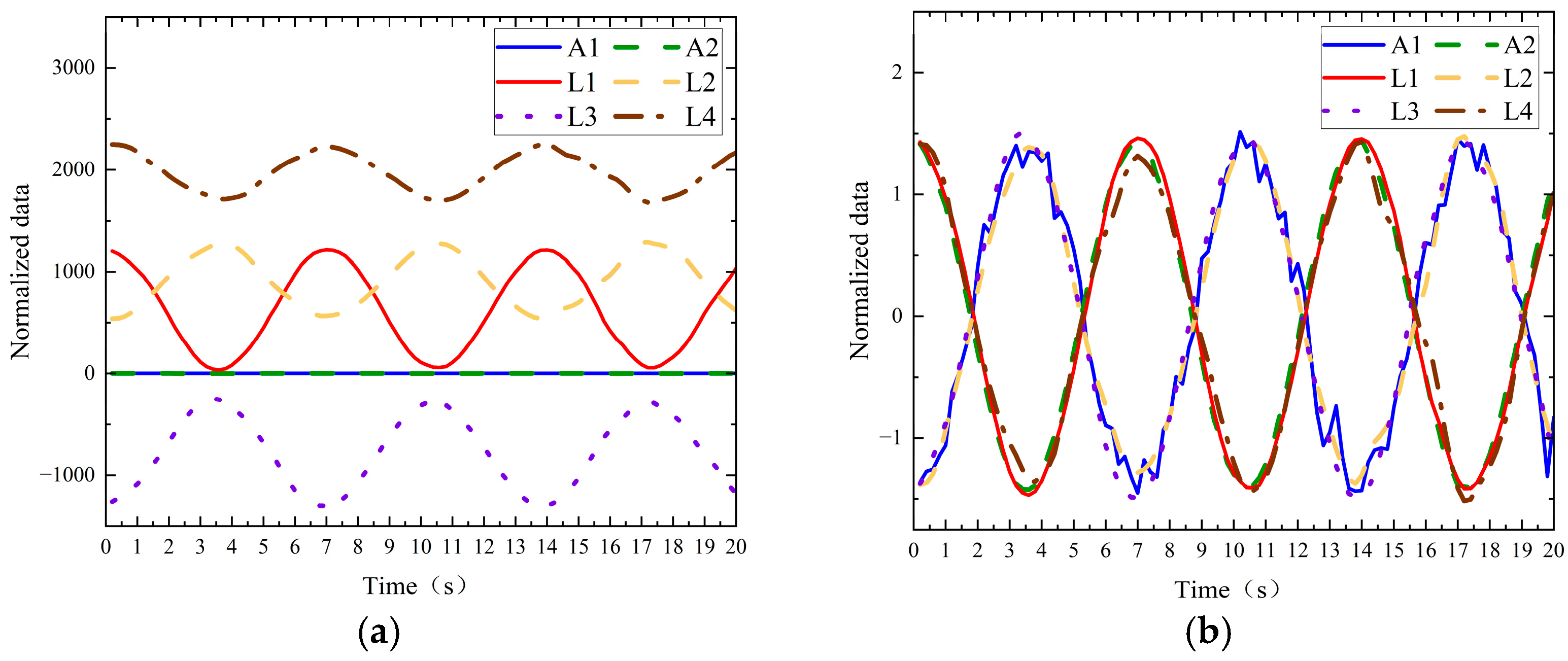
We select the acceleration sensor and the load sensor as examples. Figure 2 illustrates the curves before and after data normalization. The raw data are transformed into an effective dataset suitable for subsequent analytical tasks.

2.3. Data Correlation Processing

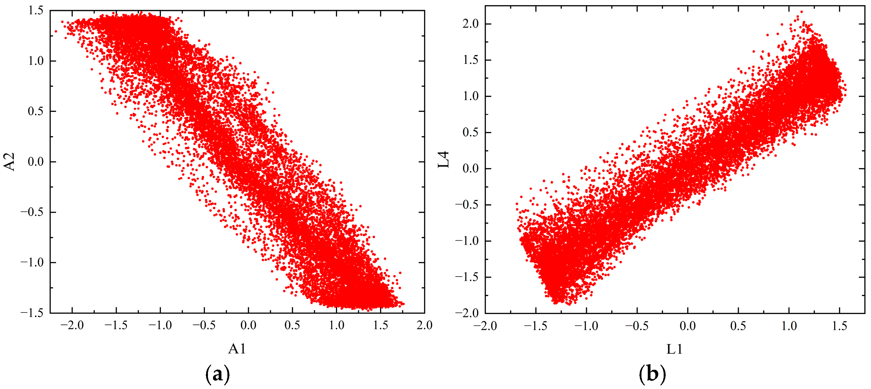
The prerequisite for employing Pearson correlation is the assumption of a linear relationship between variables. Prior to analysis, the linearity of the relationship between key parameters was preliminarily assessed through visual inspection of scatter plots. In this work, we analyze the accelerometer data and the load data as an example. The scatter distribution of 18,000 data points for A1 and A2, L1 and L4 is presented in Figure 3. The results confirmed a strong linear trend in the normalized data under normal operating conditions. Although wind turbine systems can exhibit nonlinear behaviors under faulty or extreme conditions, the primary focus of this study is on validity assessment under normal operation, where linear assumptions hold.
The correlation analysis presented in this paper utilizes the Pearson correlation coefficient that quantifies the strength and direction of the linear relationship between two variables. This coefficient is derived from the covariance and standard deviation of the variables, thereby offering an intuitive representation of their correlation degree. The formal definition of the Pearson correlation coefficient is provided in Equation (2):
P C C = i = 1 n x i x ¯ y i y ¯ Σ i = 1 n x i ˙ x ¯ 2 Σ i = 1 n y i y ¯ 2
where X = { x 1 , x 2 …, x n } and Y = { y 1 , y 2 …, y n } denotes two time series, and x ¯ = 1 n i = 1 n x i , y ¯ = 1 n i = 1 n y i . Here, the magnitude of PCC is from −1 to 1. Therein, 0 indicates no association between the two variables, while −1 and +1 represent strong negative and positive correlations, respectively [25].

3. Results and Discussion

3.1. Correlation Characteristics of Wind Turbine Monitoring Data

Figure 4 illustrates the acceleration, temperature, and load data curves for a wind turbine blade operating under normal conditions over a 20 s interval. It is evident that the fluctuation ranges of the acceleration and load curves are approximately −1.5 to 1.5, indicating that the original data fluctuations for both acceleration and load are roughly 1.5 times the standard deviation. The curves display periodic fluctuations with a period of approximately 7 s and stable amplitudes. The temperature amplitudes change between −3 and 3 with a characterization of significant fluctuations and a lack of obvious periodic variations, which suggests an absence of clear regularity. The normalized curves of A1, L2, and L3 nearly overlap, which can also be found for the curves of A2, L1, and L4. Notably, the phase of the normalized curves for A1, L2, and L3 differs by 180° relative to A2, L1, and L4. This indicates a significant correlation among A1, A2, L1, L2, L3, and L4, which somewhat results from the installation positions of the sensors. Two fiber optic acceleration sensors are positioned at one-third of the blade length on both sides of the blade, while four fiber optic load sensors are located at the blade root, evenly distributed along the circumference with an angular separation of 90° between adjacent sensors. This configuration forms a bridge measurement array to assess the load on the blade, resulting in a phase difference in the sensor monitoring data curves.
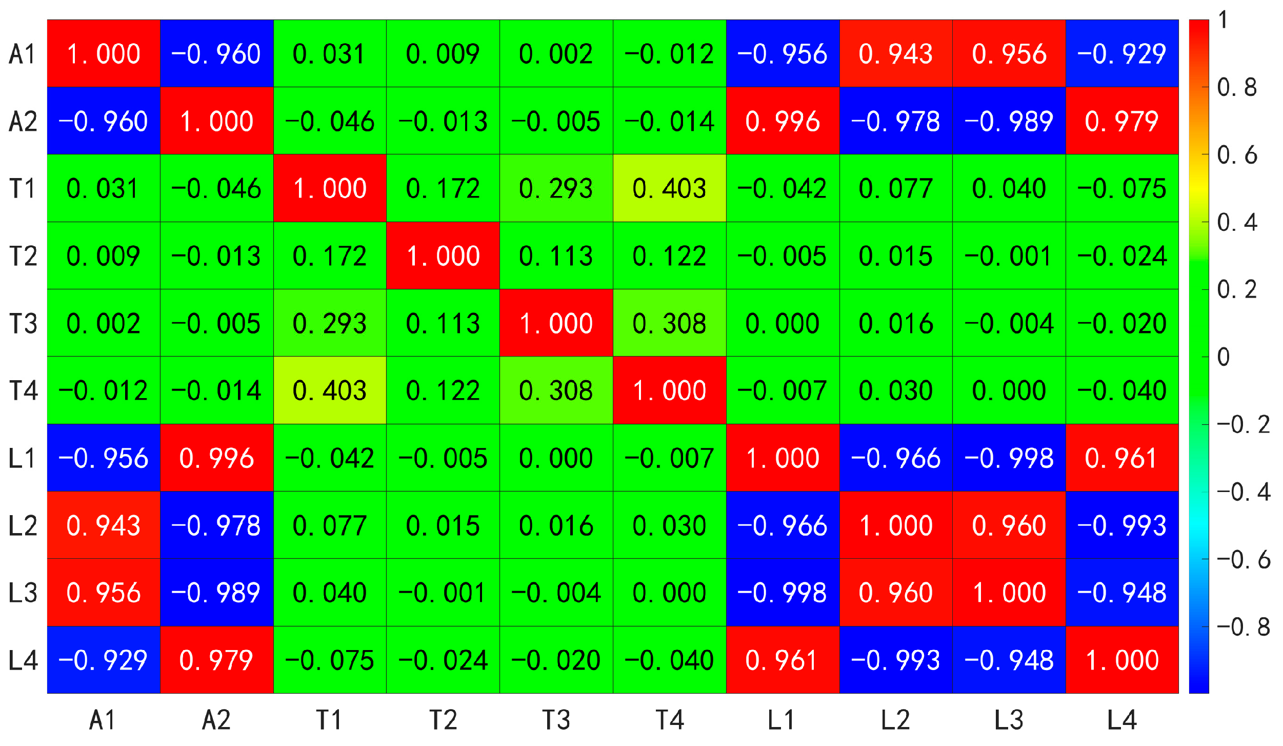
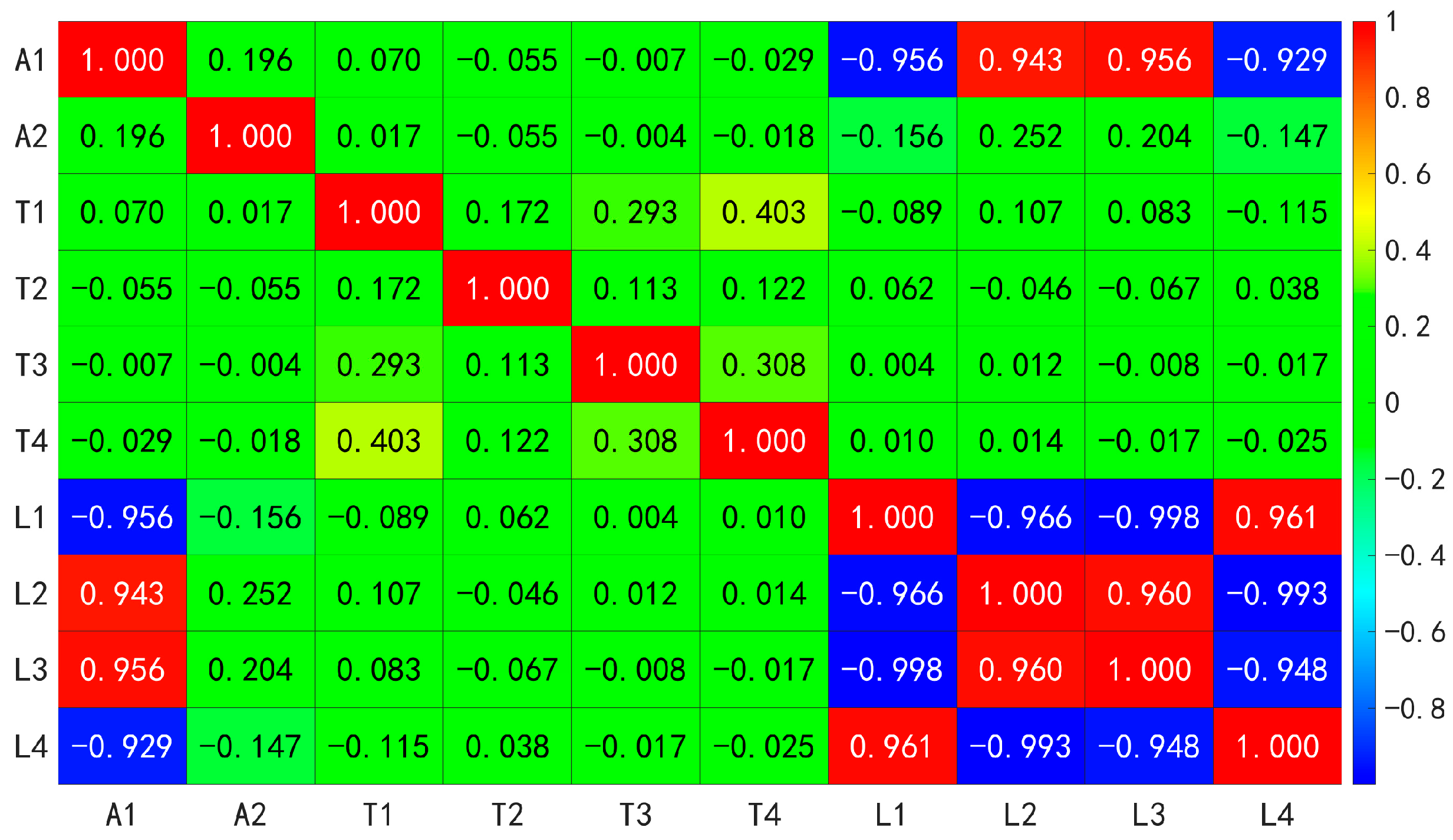
Figure 5 illustrates a heatmap of Pearson correlation coefficients among various parameters monitored over a 1 h period. Notably, positive linear correlations exist between A1 and L2, A1 and L3, A2 and L1, A2 and L4, L1 and L4, and L2 and L3, with correlation coefficients ranging from 0.943 to 0.996. This suggests that the fluctuation trends of these variables are nearly synchronized. When one variable increases, the others tend to increase as well, and conversely, when one variable decreases, the others tend to decrease. Additionally, significant negative linear correlations are observed between A1 and A2, A1 and L1, A1 and L4, A2 and L2, A2 and L3, L1 and L2, L1 and L3, L2 and L4, and L3 and L4, with correlation coefficients ranging from −0.929 to −0.998. This indicates that the fluctuation trends of these variables are largely oppositional. These findings are entirely consistent with the results in Figure 4. Given the strong correlations among the parameters, any abnormal value in a specific parameter will alter the correlation with other parameters. Thus, the validity of the data can be assessed based on the degree of association between the parameters. However, the correlation coefficients between T1, T2, T3, T4, and the other parameters range from −0.115 to 0.403, which indicates no significant correlation. Consequently, their validity cannot be determined based on the degree of association.

3.2. Impact of Filtering on the Correlation of Wind Turbine Monitoring Data

In this work, the temperature sensor measures the ambient temperature surrounding it for the purpose of error compensation in other sensors. Ideally, a strong correlation should exist between the temperatures. However, as illustrated in Figure 4, the temperature exhibits significant and irregular fluctuations. Furthermore, Figure 5 demonstrates that the correlation between these temperatures is weak. Obviously, it is different from the realistic case, which suggests that the temperature signal may be influenced by interference. Hence, it is possible to highlight the need for signal filtering prior to conducting correlation analysis.
Here, we process the data signal by a Butterworth low-pass filter [26] to reduce the effect of noise on the correlation coefficient. Figure 6 shows the temperature data curve with and without filtering. It is evident that the temperature curve prior to filtering displays significant high-frequency noise. After applying the filter, the curve becomes smooth, the high-frequency noise is eliminated, and the overall trend of the curve is clarified.
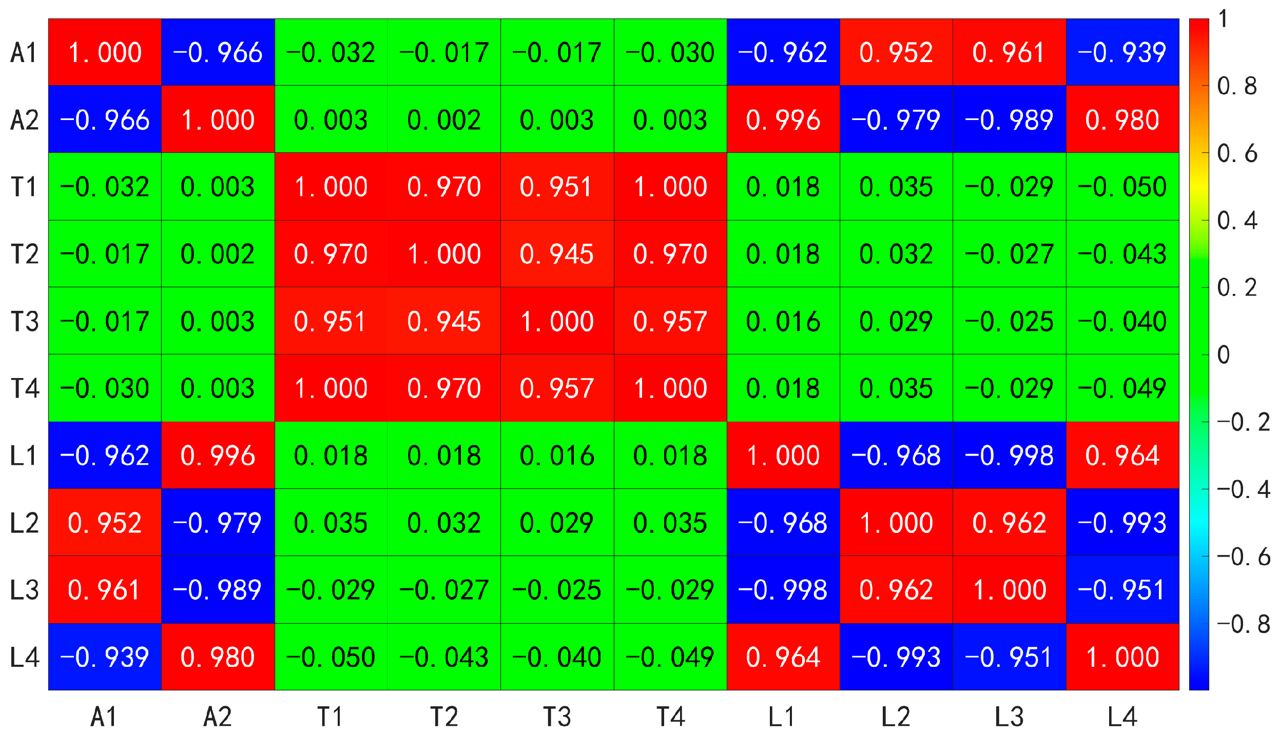
Figure 7 shows the Pearson correlation coefficient heatmap of the low-pass filtered data. The correlation coefficients among T1, T2, T3, and T4 shift from a range of 0.172 to 0.403 to a range of 0.951 to 1. This transition reflects a change from a weak to a strong correlation, which is consistent with the actual conditions observed. The results suggest that the temperature data are significantly influenced by high-frequency noise, and without appropriate filtering, the genuine correlation between the temperature datasets remains obscured, leading to a misleading impression of weak correlation. This finding underscores a substantial correlation between the temperatures, allowing for the assessment of temperature data validity based on the degree of association.
To quantitatively evaluate the enhancement effect of filtering processing on data correlation, we conducted a statistical analysis on five sets of temperature monitoring data, comparing the average PCC values of temperature sensors before and after filtering. The results are presented in Table 2. It can be observed that all PCC values after filtering exhibit a significant improvement, with an increase ranging from 35.09% to 311.06%. Moreover, the filtered data demonstrate strong correlations. This further validates the effectiveness of the filtering process in restoring the genuine correlations among the data.

3.3. Impact of Signal Phase Difference on Correlation

Here, A2 data of the wind turbine during normal operation are phase-shifted by 90°. The comparison between the original A2 data and the phase-shifted data is shown in Figure 8. The phase-shifted data are integrated with other normal data to create a comprehensive dataset. The corresponding Pearson correlation coefficient heatmap is calculated, as shown in Figure 9. It can be found that the peaks, troughs, and overall shape of the A2 data curve exhibited minimal changes, indicating that the amplitude of the data remained constant. However, Figure 9 reveals that the absolute values of the correlation coefficients between A2 and A1, L1, L2, L3, and L4 shift from a strong correlation range of 0.960 to 0.996 to a weak correlation range of 0.147 to 0.252. This indicates that the A2 data became unreliable, which contradicts the actual results. Consequently, it is imperative to adjust the phase of periodic data prior to conducting correlation analysis to avoid misjudgments.

3.4. Impact of Interference Signals on the Correlation of Monitoring Data in Wind Turbines

As previously mentioned, noise, as an interfering signal, significantly impacts the correlation with temperature. Normally, interfering signals are essentially random or non-systematic fluctuations. When an interfering signal is superimposed on an original signal, it dilutes or blurs the true associative patterns between variables, even if a strong inherent correlation exists. The presence of interfering signals causes data points to scatter more widely [27,28]. Consequently, the absolute value of the calculated correlation coefficient is lower than the true correlation coefficient. In extreme cases, strong correlations may be completely obscured by interfering signals, leading to misjudgment of uncorrelated data or weak correlation. This work will analyze the impact of two typical interfering signals of Gaussian noise and white noise on correlation.

3.4.1. Gaussian Noise Interference

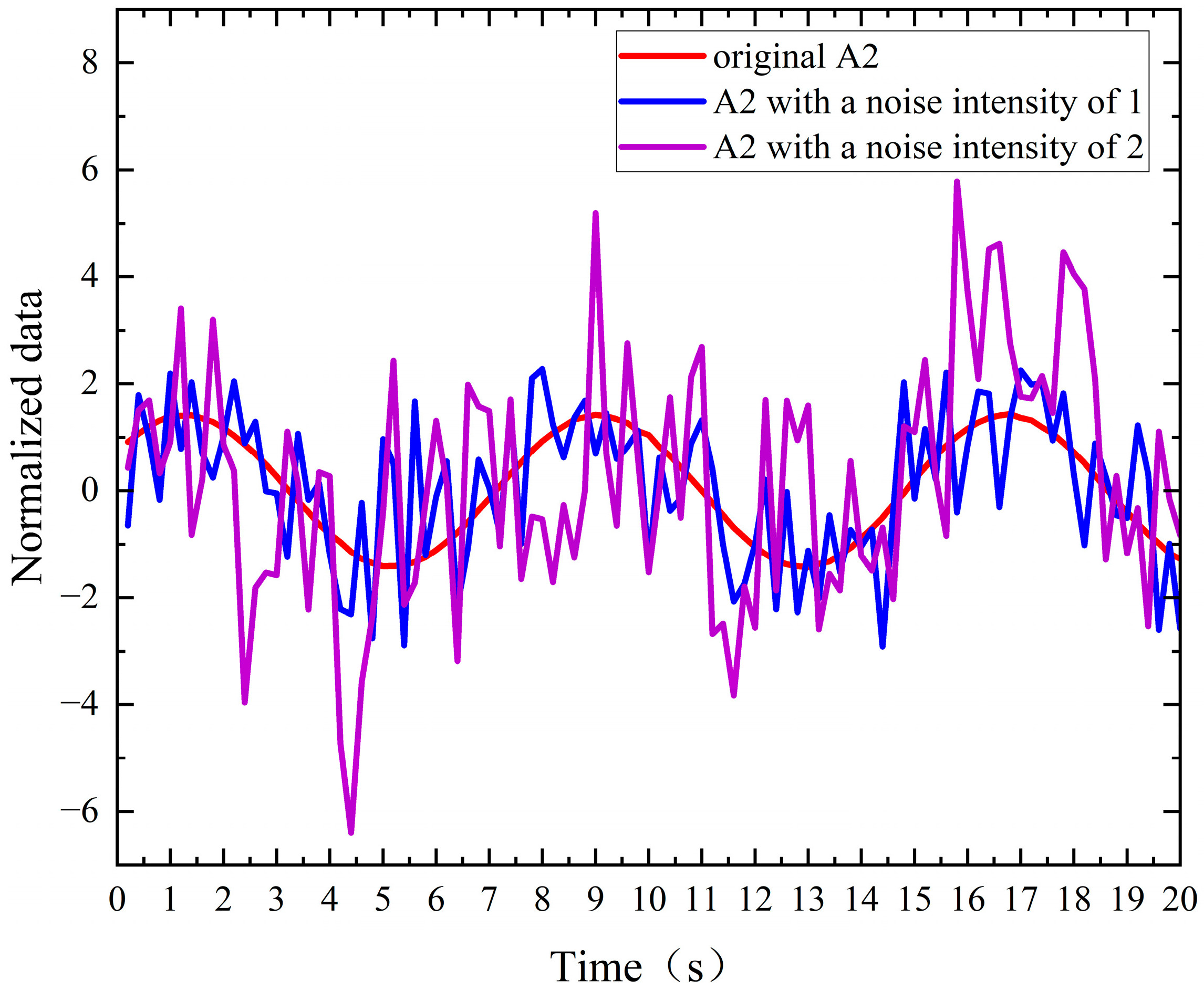
In many natural phenomena and signal processing applications, the most frequently encountered noise is a Gaussian distribution, commonly referred to as Gaussian noise [29,30,31]. During the normal operation of the wind turbine, Gaussian noises with intensity levels 1 and 2 are introduced into the A2 monitoring data. The comparison curves between the original data and the data affected by Gaussian noise are presented in Figure 10. The noise data are integrated with other normal data to form a comprehensive dataset, and the corresponding Pearson correlation coefficient heatmap is calculated, as shown in Figure 11. When the A2 data were subjected to Gaussian noise of intensity 1, the absolute values of the correlation coefficient between A2 and other parameters decrease from 0.960–0.996 to 0.679–0.699, representing a reduction of approximately 29.55%. When the A2 data are disturbed by Gaussian noise of intensity 2, the absolute value of the correlation coefficient between A2 and other originally strongly correlated parameters decreased from 0.960–0.996 to 0.430–0.444, indicating a reduction of approximately 55.32%. This suggests that as the noise intensity increases, the degree of correlation between A2 and other parameters diminishes progressively. It can be concluded that the introduction of higher intensity Gaussian noise renders the A2 data unreliable.
From a practical application perspective, the ability to identify Gaussian noise can effectively prevent misjudgment of correlations. When A2 is influenced by Gaussian noise with a certain intensity, its Pearson correlation coefficient with other strongly correlated parameters decreases in a predictable manner.
Let the original data be x and y , the formula for the original Pearson correlation coefficient can be abbreviated as ρ = cov x , y σ x σ y . By adding Gaussian noise n with a mean of 0 and a variance of σ n 2 to x , we obtain x = x + n , then the variance of x is σ x 2 = σ x 2 + σ n 2 , while the covariance remains essentially unchanged, i.e., c o v x , y = c o v x , y , so the Pearson correlation coefficient after adding Gaussian noise is: ρ = cov x , y σ x 2 + σ n 2 σ y = ρ σ x σ x 2 + σ n 2 . Transforming it yields σ n = σ x ρ 2 ρ 2 1 ; thus, the intensity of the noise σ n can be calculated.
Since the data are normalized, the standard deviation of A2 data is σ a 2 = 1 , the correlation coefficients between A1 and A2 are ρ = 0.960 and ρ = 0.679 , and the calculated σ n = 0.999 , which has an error of only 0.1% compared to the actual noise intensity σ n = 1 .

3.4.2. White Noise Interference

White noise is a random signal characterized by a power spectral density that is approximately constant across a wide frequency range and uncorrelation of value at any two distinct moments. In the time domain, it is represented as instantaneous random fluctuations with a mean of zero and a fixed variance, exhibiting an autocorrelation function in the form of an impulse. In practical applications, Gaussian white noise is the most prevalent type [32,33].
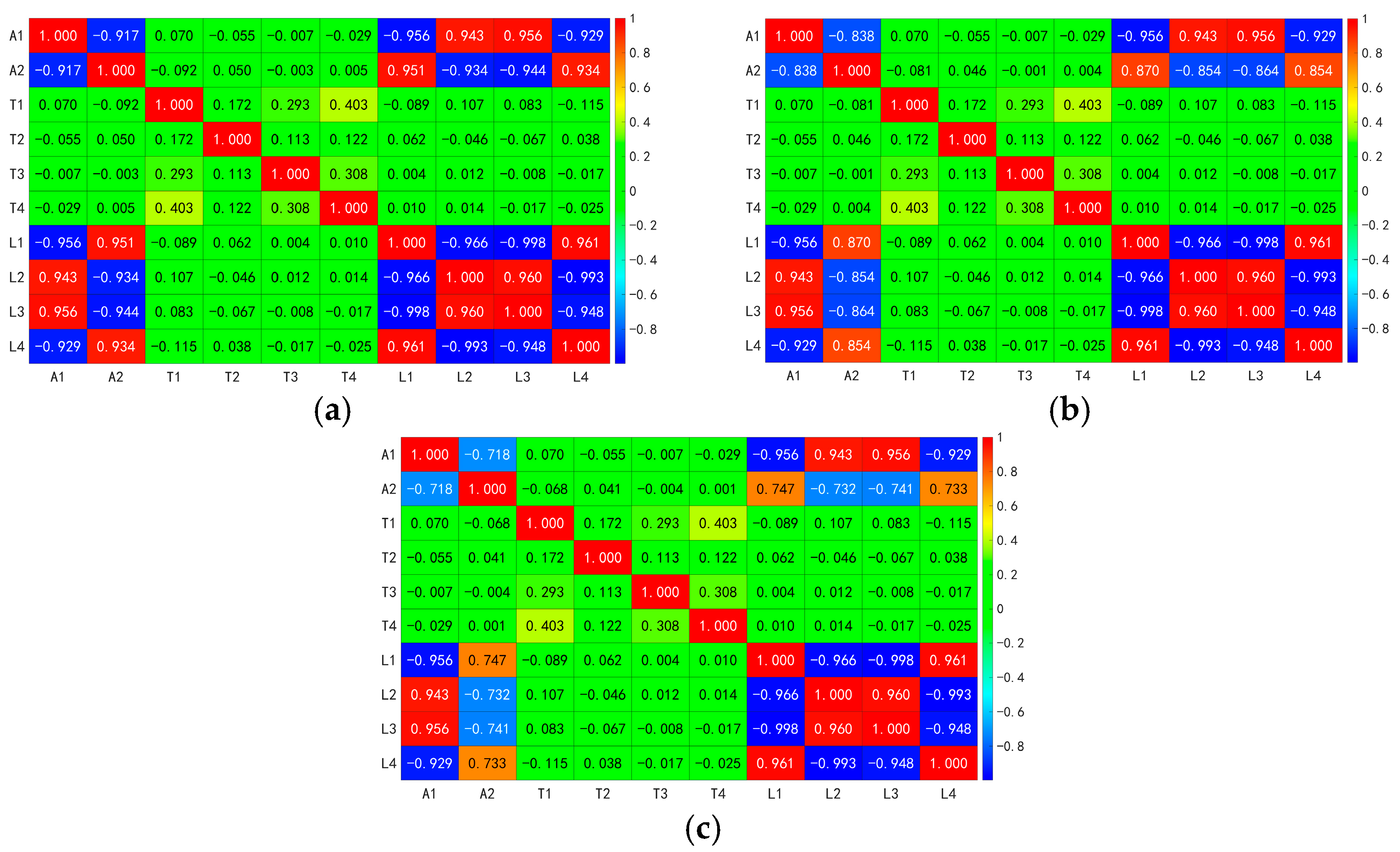
During the normal operation of the wind turbine, Gaussian white noise with signal-to-noise ratios (SNR) of 10 dB, 5 dB, and 1 dB was introduced into the A2 monitoring data. Figure 12 illustrates the comparison of the curves between the original data and the noise-interfered data. Subsequently, the noisy data are combined with other normal data to create a comprehensive dataset, from which the corresponding Pearson correlation coefficient heatmap is generated, as shown in Figure 13. For a signal-to-noise ratio of 10 dB, the absolute values of the correlation coefficients between A2 and A1, L1, L2, L3, and L4 decreased to 0.917–0.951, reflecting a reduction of approximately 4.48%. For 5 dB, these coefficients further decreased to 0.838–0.870, indicating a reduction of around 12.71%. For 1 dB, the absolute values dropped to 0.718–0.747, representing a reduction of approximately 25.21%. These data suggest that as the signal-to-noise ratio decreases, the real signal data are increasingly affected by noise, leading to a weakening of the correlation between signal data and a decline in data reliability. In other words, a lower signal-to-noise ratio corresponds to a greater interference of white noise on the signal; conversely, a higher signal-to-noise ratio enhances the ability to resist white noise interference, thereby facilitating more accurate signal identification.

4. Conclusions

This paper proposes a method for determining data validity through data correlation by utilizing the interrelationships among various parameter datasets. This approach facilitates the construction of a more accurate model for assessing data validity.
To quantify the degree of parameter association among the 10 monitoring data points of wind turbine blades, a Pearson correlation coefficient is employed. The absolute values of the correlation coefficients among A1, A2, L1, L2, L3, and L4 range from 0.929 to 0.998, while those between T1, T2, T3, and T4 range from 0.172 to 0.403. After filtering the temperature data, the results revealed an increase in the correlation coefficients to a range of 0.951 to 1, indicating that data noise significantly affects the correlation coefficients. For the periodic data, the phase of A2 data shifts by 90°, resulting in changing the absolute values of the correlation coefficients between A2 and A1, L1, L2, L3, and L4 from a strong correlation of 0.960 to 0.996 to a weak correlation of 0.147 to 0.252. Thus, the data phase has a significant impact on correlation analysis. When Gaussian noise with intensities of 1 and 2 is applied to A2, the absolute values of correlation coefficients between A2 and other parameters decrease by 29.55% to 55.32%, respectively. This indicates that stronger Gaussian noise intensities lead to a greater reduction in the degree of correlation, resulting in lower correlation coefficients. Additionally, when Gaussian white noise with signal-to-noise ratios of 10 dB, 5 dB, and 1 dB was applied to A2, the absolute values of the correlation coefficients between A2 and other parameters decreased by approximately 4.48%, 12.71%, and 25.21%, respectively, demonstrating that a lower signal-to-noise ratio intensifies the interference of white noise on the signal.
In summary, noise, phase, and interference significantly impact the correlation relationships among data. Therefore, it is essential to effectively filter the data to mitigate the influence of interfering signals on correlation analysis. By conducting a stable correlation analysis, the validity of wind turbine monitoring data can be assessed by monitoring anomalies in the correlation coefficients.

Author Contributions

Conceptualization, G.C., N.C. and D.H.; Methodology, G.C.; Software, G.C.; Validation, N.C. and X.N.; Formal analysis, G.C.; Investigation, G. C. and X.N.; Resources, N.C., X.N. and D.H.; Data curation, X.N.; Writing—original draft, G.C.; Writing—review & editing, N.C.; Visualization, G.C.; Supervision, N.C. and D.H.; Funding acquisition, N.C. All authors have read and agreed to the published version of the manuscript.

Funding

This research was funded by National Key R & D Program of China (2023YFB4203304), Science and Technology Commission of Shanghai Municipality Grant No. 24DZ3000803, and the non-carbon energy conversion and utilization institute under the Shanghai Class IV Peak Disciplinary Development Program.

Institutional Review Board Statement

Not applicable.

Informed Consent Statement

Not applicable.

Data Availability Statement

The datasets presented in this article are not readily available due to technical limitation.

Conflicts of Interest

The authors declare no conflict of interest.

References

  1. Heffernan, O. The Third Industrial Revolution: How Lateral Power is Transforming Energy, the Economy, and the World. Nat. Clim. Chang. 2012, 2, 67–68. [Google Scholar] [CrossRef]
  2. Zou, C.E.; Li, S.X.; Xiong, B.; Liu, H.L.; Ma, F. Revolution and significance of “Green Energy Transition” in the context of new quality productive forces: A discussion on theoretical understanding of “Energy Triangle”. Pet. Explor. Dev. 2024, 51, 1611–1627. [Google Scholar] [CrossRef]
  3. Holechek, J.L.; Geli, H.M.E.; Sawalhah, M.N.; Valdez, R. A Global Assessment: Can Renewable Energy Replace Fossil Fuels by 2050? Sustainability 2022, 14, 4792. [Google Scholar] [CrossRef]
  4. Sayed, E.T.; Olabi, A.G.; Alami, A.H.; Radwan, A.; Mdallal, A.; Rezk, A.; Abdelkareem, M.A. Renewable Energy and Energy Storage Systems. Energies 2023, 16, 1415. [Google Scholar] [CrossRef]
  5. Liu, C.-J.; Lu, J.-Y.; Zhao, W.-C.; Xu, Q.; Jin, Y.-J. Development Scenarios and Environmental Benefits Analysis of Future Power Generation Industry Under Two Modes in China. Huan Jing Ke Xue = Huanjing Kexue 2022, 43, 3375–3385. [Google Scholar] [CrossRef] [PubMed]
  6. Avtar, R.; Sahu, N.; Aggarwal, A.K.; Chakraborty, S.; Kharrazi, A.; Yunus, A.P.; Dou, J.; Kurniawan, T.A. Exploring Renewable Energy Resources Using Remote Sensing and GIS—A Review. Resources 2019, 8, 149. [Google Scholar] [CrossRef]
  7. Wang, Y.J.; Wang, R.; Tanaka, K.; Ciais, P.; Penuelas, J.; Balkanski, Y.; Sardans, J.; Hauglustaine, D.; Liu, W.; Xing, X.F.; et al. Accelerating the energy transition towards photovoltaic and wind in China. Nature 2023, 619, 761–767. [Google Scholar] [CrossRef]
  8. Mishnaevsky, L.; Branner, K.; Petersen, H.N.; Beauson, J.; McGugan, M.; Sørensen, B.F. Materials for Wind Turbine Blades: An Overview. Materials 2017, 10, 1285. [Google Scholar] [CrossRef] [PubMed]
  9. Tchakoua, P.; Wamkeue, R.; Ouhrouche, M.; Slaoui-Hasnaoui, F.; Tameghe, T.A.; Ekemb, G. Wind Turbine Condition Monitoring: State-of-the-Art Review, New Trends, and Future Challenges. Energies 2014, 7, 2595–2630. [Google Scholar] [CrossRef]
  10. Hong, S.; McMorland, J.; Zhang, H.X.; Collu, M.; Halse, K.H. Floating offshore wind farm installation, challenges and opportunities: A comprehensive survey. Ocean Eng. 2024, 304, 117793. [Google Scholar] [CrossRef]
  11. Liu, W.Y.; Tang, B.P.; Han, J.G.; Lu, X.N.; Hu, N.N.; He, Z.Z. The structure healthy condition monitoring and fault diagnosis methods in wind turbines: A review. Renew. Sust. Energy Rev. 2015, 44, 466–472. [Google Scholar] [CrossRef]
  12. Gowda, M.C.M.; Mallikarjun, N.P.; Gowda, P.; Chandrashekhar, R. Improvement of the Performance of Wind Turbine Generator Using Condition Monitoring Techniques. In Proceedings of the 7th International Conference on Intelligent Systems and Control (ISCO), Coimbatore, India, 4–5 January 2013; pp. 495–501. [Google Scholar]
  13. Niu, Z.X.; Shi, S.P.; Sun, J.Y.; He, X. A Survey of Outlier Detection Methodologies and Their Applications. In Proceedings of the 3rd International Conference on Artificial Intelligence and Computational Intelligence (AICI 2011), Taiyuan, China, 23–25 September 2011; pp. 380–387. [Google Scholar]
  14. Gao, P.; Wu, T.J.; Ge, Y.; Yang, G.; Lu, Y.F. Correcting the nighttime lighting data underestimation effect based on light source detection and luminance reconstruction. Int. J. Appl. Earth Obs. Geoinf. 2023, 121, 103380. [Google Scholar] [CrossRef]
  15. Liu, S.F.; Tao, Y.; Xie, N.M.; Tao, L.Y.; Hu, M.L. Advance in grey system theory and applications in science and engineering. Grey Syst. 2022, 12, 804–823. [Google Scholar] [CrossRef]
  16. Xiao, C.W.; Ye, J.Q.; Esteves, R.M.; Rong, C.M. Using Spearman’s correlation coefficients for exploratory data analysis on big dataset. Concurr. Comput.-Pract. Exp. 2016, 28, 3866–3878. [Google Scholar] [CrossRef]
  17. Zheng, K.; Fang, J.; Li, J.; Shi, H.; Xu, Y.; Li, R.; Xie, R.; Cai, G. Robust Grey Relational Analysis-Based Accuracy Evaluation Method. Appl. Sci. 2025, 15, 4926. [Google Scholar] [CrossRef]
  18. Liu, P.F.; Wang, S.C.; Zhao, P. Robust estimation and test for Pearson’s correlation coefficient. Random Matrices-Theor. Appl. 2024, 13, 17. [Google Scholar] [CrossRef]
  19. Phillips, T.; GauthierDickey, C.; Thurimella, R. Using Transitivity to Increase the Accuracy of Sample-Based Pearson Correlation Coefficients. In Proceedings of the 12th International Conference on Data Warehousing and Knowledge Discovery, Bilbao, Spain, 30 August–3 September 2010; pp. 157–171. [Google Scholar]
  20. Wharton, S.; Lundquist, J.K. Atmospheric stability affects wind turbine power collection. Environ. Res. Lett. 2012, 7, 9. [Google Scholar] [CrossRef]
  21. Fernandez-Díaz, A. Overview and Perspectives of Chaos Theory and Its Applications in Economics. Mathematics 2024, 12, 20. [Google Scholar] [CrossRef]
  22. Barker, P.M.; McDougall, T.J. Two Interpolation Methods Using Multiply-Rotated Piecewise Cubic Hermite Interpolating Polynomials. J. Atmos. Ocean. Technol. 2020, 37, 605–619. [Google Scholar] [CrossRef]
  23. Kim, B.S.; Lee, S.; Rha, S.Y.; Chung, H.C. cDNA Microarray Experiment: Design Issues in Early Stage and the Need of Normalization. Cancer Res. Treat. Off. J. Korean Cancer Assoc. 2003, 35, 533–540. [Google Scholar] [CrossRef]
  24. Huang, J.L.; Li, Y.F.; Keung, J.W.; Yu, Y.T.; Chan, W.K. An Empirical Analysis of Three-stage Data-Preprocessing for Analogy-based Software Effort Estimation on the ISBSG Data. In Proceedings of the IEEE International Conference on Software Quality, Reliability and Security (Companion Volume), Prague, Czech Republic, 25–29 July 2017; pp. 442–449. [Google Scholar]
  25. Wang, D.M.; Cao, C.Y.; Chen, N.C.; Pan, W.G.; Li, H.C.; Wang, X.D. A correlation-graph-CNN method for fault diagnosis of wind turbine based on state tracking and data driving model. Sustain. Energy Technol. Assess. 2023, 56, 102995. [Google Scholar] [CrossRef]
  26. Hu, X.; Liu, W.; Huo, H. An intelligent network traffic prediction method based on Butterworth filter and CNN–LSTM. Comput. Netw. 2024, 240, 110172. [Google Scholar] [CrossRef]
  27. Han, X. Artificial Intelligence-based Interference Signal Recognition for Satellite Communications. In Proceedings of the 2024 International Conference on Advanced Control Systems and Automation Technologies, ACSAT 2024, Nanjing, China, 15–17 November 2024; pp. 279–282. [Google Scholar]
  28. Dutta, S.; Boongoen, T.; Zwiggelaar, R. Human Activity Recognition with Noise-Injected Time-Distributed AlexNet. Biomimetics 2025, 10, 613. [Google Scholar] [CrossRef]
  29. Alfatemi, A.; Oliveira, D.; Rahouti, M.; Hafid, A.; Ghani, N. Precision DDoS Detection through Gaussian Noise-Augmented Neural Networks. In Proceedings of the 15th International Conference on Network of the Future, NoF 2024, Barcelona, Spain, 2–4 October 2024; pp. 178–185. [Google Scholar]
  30. Ghazdali, A.; Hadri, A.; Laghrib, A.; Nachaoui, M. Poisson noise and Gaussian noise separation through copula theory. Multimed. Tools Appl. 2024, 83, 67927–67952. [Google Scholar] [CrossRef]
  31. Bahador, F.G.; Mokhtary, P.; Lakestani, M. Mixed Poisson-Gaussian noise reduction using a time-space fractional differential equations. Inf. Sci. 2023, 647, 15. [Google Scholar] [CrossRef]
  32. Jia, L.; Li, S.; Kou, L.; Wu, K. Homoclinic Bifurcations and Chaotic Dynamics in a Bistable Vibro-Impact SD Oscillator Subject to Gaussian White Noise. Int. J. Bifurc. Chaos 2024, 34, 2450077. [Google Scholar] [CrossRef]
  33. Qiao, G.-R.; Bai, B.; Weng, Z.-X.; Wu, J.-Y.; Nie, Y.-Q.; Zhang, J. White Gaussian Noise Generation with a Vacuum State Quantum Entropy Source Chip. IEEE J. Sel. Top. Quantum Electron. 2025, 31, 9200108. [Google Scholar] [CrossRef]
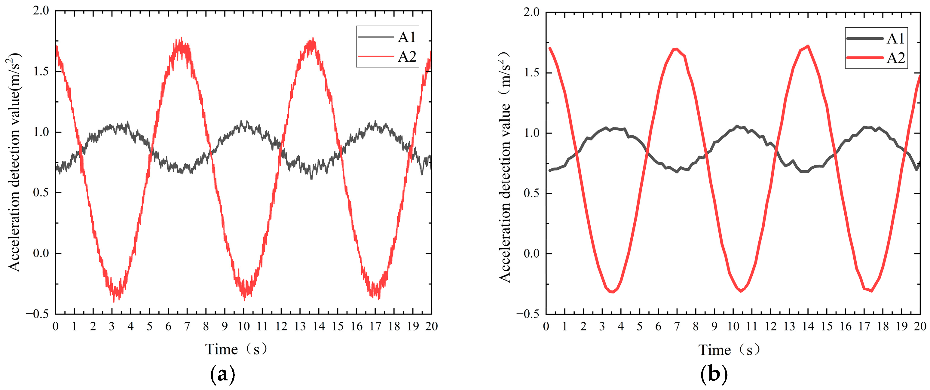
Figure 1. Curves of acceleration data before (a) and after (b) downsampling.
Applsci 15 10320 g001
Figure 2. Curves of acceleration and load data before (a) and after (b) normalization processing.
Applsci 15 10320 g002
Figure 3. Scatter plot of the accelerometer data (a) and the load date (b).
Applsci 15 10320 g003
Figure 4. The data curve under normal operating conditions.
Applsci 15 10320 g004
Figure 5. Heatmap of Pearson correlation coefficients under normal operating conditions.
Applsci 15 10320 g005
Figure 6. The curves of temperature data before (a) and after (b) filtering processing.
Applsci 15 10320 g006
Figure 7. Heatmap of the filtered Pearson correlation coefficients.
Applsci 15 10320 g007
Figure 8. The curve of original A2 and phase-shifted A2.
Applsci 15 10320 g008
Figure 9. Heatmap of Pearson correlation coefficients for A2 data curve phase shifts.
Applsci 15 10320 g009
Figure 10. Comparison of the curves between original A2 and Gaussian noise A2.
Applsci 15 10320 g010
Figure 11. Heatmap of Pearson correlation coefficients for A2 under Gaussian noise intensities of (a) 1 and (b) 2.
Applsci 15 10320 g011
Figure 12. Comparison of the curves between original A2 and white noise A2.
Applsci 15 10320 g012
Figure 13. The Pearson correlation coefficient heatmap of A2 under white noise intensities of (a) 10 dB, (b) 5 dB, and (c) 1 dB.
Applsci 15 10320 g013
Table 1. Nomenclature.
Nomenclature
A1Acceleration detection value 1T4Temperature detection value 4
A2Acceleration detection value 2L1Load detection value 1
T1Temperature detection value 1L2Load detection value 2
T2Temperature detection value 2L3Load detection value 3
T3Temperature detection value 3L4Load detection value 4
Table 2. Comparison of the average PCC for temperature sensor data before and after filtering.
No.Avg. PCC (Before Filtering)Avg. PCC (After Filtering)Percentage Improvement (%)
10.2350.966311.06
20.3020.821171.85
30.3440.850147.09
40.5370.92472.07
50.7380.99735.09
Disclaimer/Publisher’s Note: The statements, opinions and data contained in all publications are solely those of the individual author(s) and contributor(s) and not of MDPI and/or the editor(s). MDPI and/or the editor(s) disclaim responsibility for any injury to people or property resulting from any ideas, methods, instructions or products referred to in the content.