Behavioral Modeling of RF Power Amplifiers with Carrier-Frequency Generalization Using Interpolated Memory Polynomials

Abstract

Power amplifier behavioral modeling is an important technique for efficient and accurate digital predistortion, but conventional models fail to generalize when applied across varying carrier frequencies. This work addresses the carrier-frequency generalization by proposing a parameterized memory polynomial (PMP) modeling approach. The method involves extracting memory polynomial models at multiple carrier frequencies and interpolating their coefficients using spline interpolation, resulting in a single model capable of operating across a wide carrier-frequency band. Experimental validation was conducted using measured input–output PA responses over the 3.3–3.8 GHz range. Results obtained show that PMP built on three carrier frequencies achieves up to 9 dB average NMSE improvement compared to the fixed-coefficient MP model. The proposed model nearly matches the accuracy of the MP model at the entire measured range. The overall accuracy depends on the combination of the introduced interpolation error and the discrepancy between the initial MP model fitting errors. The proposed method offers a practical solution for PA modeling in systems requiring fast frequency agility, such as carrier aggregation and dynamic spectrum access, eliminating the need for model retraining at each operating frequency.

1. Introduction

A power amplifier (PA) is a critical component in modern wireless communication systems. It is well known that PAs are constrained by a fundamental trade-off between energy efficiency and the linearity of their transfer characteristics. High efficiency is desirable to minimize power consumption, while greater linearity ensures reduced signal distortion. Achieving high efficiency often requires operating a PA near its saturation region, where nonlinear distortions become significant. These distortions degrade signal quality, leading to higher error rates and preventing the use of more spectrally efficient modulation schemes. Conversely, maintaining high linearity forces the PA to operate in a less efficient region of its transfer characteristic, resulting in increased power consumption. This trade-off is particularly challenging in modern communication systems, where both energy efficiency and signal fidelity are critical.

The most common approach to addressing this trade-off is to linearize the nonlinear transfer characteristic of an efficient PA [1]. Numerous methods exist for achieving this, including solutions in both the analog domain (e.g., feedforward [2], feedback [3], analog predistortion [4]) and the digital domain (e.g., digital predistortion, DPD) [5]. Among these, the DPD is the most widely used method today [6]. In the DPD, the transfer characteristic of the PA is replicated in the digital domain, and a filter with an inverse transfer characteristic is constructed. Ideally, the distortions introduced by the DPD cancel out the distortions produced by the PA, resulting in a linearized output. The effectiveness of the DPD depends heavily on the accuracy of the PA characterization and modeling processes.

There are different modeling approaches. One of the most popular approaches today is behavioral modeling. A behavioral model is a simplified model that describes the essential relationship between inputs and outputs of a device or a system [7]. In contrast, an analytical model includes physical insight into the modeled system, which enables accurate prediction of the behavior of a system across different operational conditions. This generality comes with a cost, as such models are often computationally expensive and impractical in real-time systems. Behavioral models aim to reduce computational costs by characterizing the system at a limited range of operating conditions. For the purposes of DPD linearization, where computational costs play a major role, the PA behavioral modeling has become a widespread technique. The drawback of the behavioral model, however, is that it is not reliable outside of the conditions for which it was extracted. These conditions include drive level, modulation bandwidth, peak-to-average power ratio (PAPR), temperature, and frequency.

One of the challenges in behavioral modeling of power amplifiers is to achieve generalization across different carrier frequencies. Typically, the behavioral models are trained and used on a certain carrier frequency or a set of carrier frequencies. A model capable of accurately representing the PA behavior across a continuous range of carrier frequencies could be valuable in several areas. For example, it may benefit systems that frequently switch between different carrier frequencies, such as cognitive radio and dynamic spectrum access systems, where transceivers must rapidly transition between non-contiguous frequency bands without requiring the model to retrain or reload.

In this paper, the authors aim to specifically investigate the effect of carrier-frequency variation on behavioral model accuracy and propose a model capable of operating across a wide range of frequencies. Previous research has examined this effect [8], including a neural network approach [9]. The latter study proposes a neural network architecture that aims to generalize a PA model across several carrier frequencies. There are modeling approaches focused on data collection across different carrier frequencies (e.g., [10]). In a broader context of behavioral modeling, a certain trend toward model generalization can be observed currently. For instance, the authors of [11] propose an incremental bandwidth and frequency-dependent (IBWFD) generalized memory polynomial approach, based on a combination of stationary and adjustable DPD implementations. In [12], the authors demonstrate the capability of enabling dynamic adaptation to varying-resource block allocations in 5G NR systems. An efficient DPD implementation based on look-up-table values for interpolation was proposed in [13]. Although focused on different topics, these studies highlight increasing interest in frequency-adaptive modeling techniques such as adaptive blocks, spline interpolation, or dynamic coefficient adaptation.

This paper introduces a parametric memory polynomial (PMP) model where each coefficient is parameterized as a continuous function of carrier frequency. By estimating MP models at anchor frequencies and interpolating the resulting coefficients, the method achieves improvements in the NMSE (up to 11 dB gain versus standard MP across a 3.3–3.8 GHz band). The key contributions are the following:

• A novel frequency-parameterized memory polynomial (PMP) model is proposed, where each coefficient is represented as a continuous function of the carrier frequency. This provides a single, unified model that accurately generalizes across a wide operational bandwidth, eliminating the need for a bank of narrowband models.
• The proposed methodology is computationally efficient. The significant processing overhead is confined to an offline training phase, while the runtime computational cost is equivalent to evaluating a standard memory polynomial, making it a practical and viable solution for real-time digital predistortion systems.
• We identify, demonstrate, and analyze fundamental limitations of any such parametrization approach. The performance is ultimately bounded by the accuracy and consistency of the underlying single-frequency models. We directly link performance saturation and error oscillation to discrepancies in these initial models caused by frequency-dependent behavioral regimes of the PA.
• The method is rigorously validated on a commercial PA across the 3.3–3.8 GHz band. The results demonstrate a substantial performance improvement, achieving up to a 14 dB reduction in the NMSE over a conventional single-frequency model when generalizing across the entire bandwidth.

The present paper is organized as follows: Section 1 is an introduction. Section 2 focuses on modeling and measurement techniques. Section 3 demonstrates the results obtained. Section 4 discusses the results. Section 5 provides the conclusions. References are provided at the end of the article.

2. Modeling and Measurement Technique

The memory polynomial model is an established approach in the RF power amplifier behavioral modeling, offering an effective compromise between computational efficiency and modeling accuracy. The MP model is mathematically defined as [14]:

$$y_{\mathrm{M}\mathrm{P}}\left(n\right)=\sum _{k=0}^{K-1}\sum _{m=0}^{M-1}{a}_{km}x\left(n-m\right){\left|x\left(n-m\right)\right|}^k,$$

(1)

where $x\left(n\right)$ represents the baseband excitation signal, $y_{\mathrm{M}\mathrm{P}}\left(n\right)$ denotes the power amplifier’s output as predicted by the memory polynomial model, and $a_{km}$ are model coefficients. The “memory” designation reflects the model’s incorporation of both current and past input values to determine the PA’s response. This memory effect is explicitly captured through the inclusion of delayed input samples in the model structure.

The model extraction process involves computing the coefficient set $a_{km}$ that satisfies Equation (1) when both input excitation and output response signals are known. These coefficients are determined by solving for the least square error (LSE) solution that minimizes the discrepancy between the measured output $y$ and the prediction by the model $y_{\mathrm{M}\mathrm{P}}$. For a dataset of N signal samples, the model’s predictive accuracy is typically evaluated using metrics such as the normalized mean square error (NMSE):

$$NMSE={\displaystyle \frac{\frac{1}{N}\sum {\left|y-y_{MP}\right|}^2}{\frac{1}{N}\sum {\left|y\right|}^2}}.$$

(2)

The achieved modeling accuracy primarily depends on both the characteristics of the modeled system and the selected model parameters.

The formulation in Equation (1) makes no explicit reference to carrier frequency or other specific operating parameters. This formulation implicitly assumes that the training data adequately represent the class of input signals that the amplifier will encounter. Furthermore, such models are typically trained using baseband data—the demodulated equivalent of the actual RF signals transmitted to and received from the PA. However, as demonstrated in [8], the PA behavior exhibits significant carrier-frequency dependence. Consequently, applying a model extracted at one carrier frequency to predict responses at different frequencies will inherently introduce prediction errors. This will be later confirmed by the experimental results.

To improve the MP model’s performance across varying carrier frequencies, a parametrization technique is proposed:

$$y_{\mathrm{P}\mathrm{M}\mathrm{P}}\left(n,f_c\right)=\sum _{k=0}^{K-1}\sum _{m=0}^{M-1}{p}_{km}\left(f_c\right)x\left(n-m\right){\left|x\left(n-m\right)\right|}^k.$$

(3)

where the conventional frequency-independent coefficients $a_{km}$ are replaced with frequency-dependent functions $p_{km}(f_c)$. These parametric functions are derived through the following methodological steps:

• Conduct N measurements at distinct carrier frequencies f_c, obtaining corresponding excitation-response pairs:

  $$\left\{x_{{CF}_1},y_{{CF}_1}\right\},\left\{x_{{CF}_2},y_{{CF}_2}\right\}, \dots \left\{x_{{CF}_N},y_{{CF}_N}\right\}.$$

  (4)
• For each dataset, extract a standard MP model, yielding N coefficient sets:

  $$\mathrm{A}(f_{c_0})=\left[\begin{array}{c}{a}_{00}\\ a_{01}\\ ⋮\\ a_{km}\end{array}\right],\hspace{1em}\hspace{1em}\mathrm{A}(f_{c_1})=\left[\begin{array}{c}{b}_{00}\\ b_{01}\\ ⋮\\ b_{km}\end{array}\right],\hspace{1em}\hspace{1em}\dots \mathrm{A}(f_{c_N})=\left[\begin{array}{c}{c}_{00}\\ c_{01}\\ ⋮\\ c_{km}\end{array}\right].$$

  (5)
• Apply interpolation to generate continuous coefficient functions:

$$\left\{\begin{array}{c}{p}_{00}\left(f_c\right)= F_{int}\left[\right(a_{00};f_{c_0}),(b_{00};f_{c_1})\dots (c_{00};f_{c_N}\left)\right]\\ p_{01}\left(f_c\right)= F_{int}\left[\right(a_{01};f_{c_0}),(b_{01};f_{c_1})\dots (c_{01};f_{c_N}\left)\right]\\ ⋮\\ p_{km}\left(f_c\right)= F_{int}[\left(a_{km};f_{c_0}\right),\left(b_{km};f_{c_1}\right)\dots \left(c_{km};f_{c_N}\right)]\end{array}\right..$$

(6)

The method assumes sufficiently smooth PA behavior across the operational bandwidth (i.e., there are no resonances or other reasons for sharp behavior changes). Under this condition, the PMP model can accurately predict amplifier behavior at arbitrary frequencies within the characterized range, including untested frequencies between measurement points.

Several interpolation methods exist for approximating functions from discrete data points. The simplest approach, linear interpolation, constructs piecewise linear connections between points. While computationally efficient, this method yields non-smooth functions that often poorly approximate the underlying relationship unless an impractically large number of points is used. For applications requiring accurate modeling of physical processes, polynomial interpolation is generally more suitable. This method generates a smooth polynomial function when given at least k*m + 1 data points, producing a continuous representation of the form:

$$p_{km}\left(f_c\right)= {\phi }_0+{\phi }_1{f}_c+{\phi }_2{f}_c^2+\cdots +{\phi }_{\left(k\ast m\right)}{f}_c^{\left(k\ast m\right)},$$

(7)

where ${[\phi }_0\dots {\phi }_{\left(k\ast m\right)}]$ is an array of polynomial coefficients, obtained from solving a system of linear equations:

$$\left\{\begin{array}{c}{a}_{00}= {\phi }_0+{\phi }_1{f}_{c_0}+{\phi }_2{f}_{c_0}^2+\cdots +{\phi }_{\left(k\ast m\right)}{f}_{c_0}^{\left(k\ast m\right)}\\ b_{00}= {\phi }_0+{\phi }_1{f}_{c_1}+{\phi }_2{f}_{c_1}^2+\cdots +{\phi }_{\left(k\ast m\right)}{f}_{c_1}^{\left(k\ast m\right)}\\ ⋮\\ c_{00}= {\phi }_0+{\phi }_1{f}_{c_N}+{\phi }_2{f}_{c_N}^2+\cdots +{\phi }_{\left(k\ast m\right)}{f}_{c_N}^{\left(k\ast m\right)}\end{array}.\right.$$

(8)

The solution of this system of equations can be computationally optimized through established techniques such as Lagrange interpolation or Newton’s divided difference method [15]. However, this polynomial interpolation approach suffers from a fundamental limitation: the solution becomes increasingly unstable as the number of data points grows. This instability stems from the higher-order terms required in Equation (7) when interpolating more points, leading to severe oscillations known as Runge’s phenomenon. In practice, polynomial interpolation remains reliable only for modest numbers of points (typically 8–10), and in some cases, oscillatory artifacts may appear even with fewer interpolation points.

To circumvent the instability associated with high-order polynomials, the proposed method employed cubic spline interpolation [15]. This technique partitioned the dataset into subintervals and fitted a unique cubic polynomial to each segment. The resulting composite function achieved global smoothness by enforcing continuity in both the first and second derivatives at the connecting knots between adjacent splines. The complete set of spline functions was subsequently determined by solving a system of linear equations derived from these continuity conditions and the specified boundary conditions.

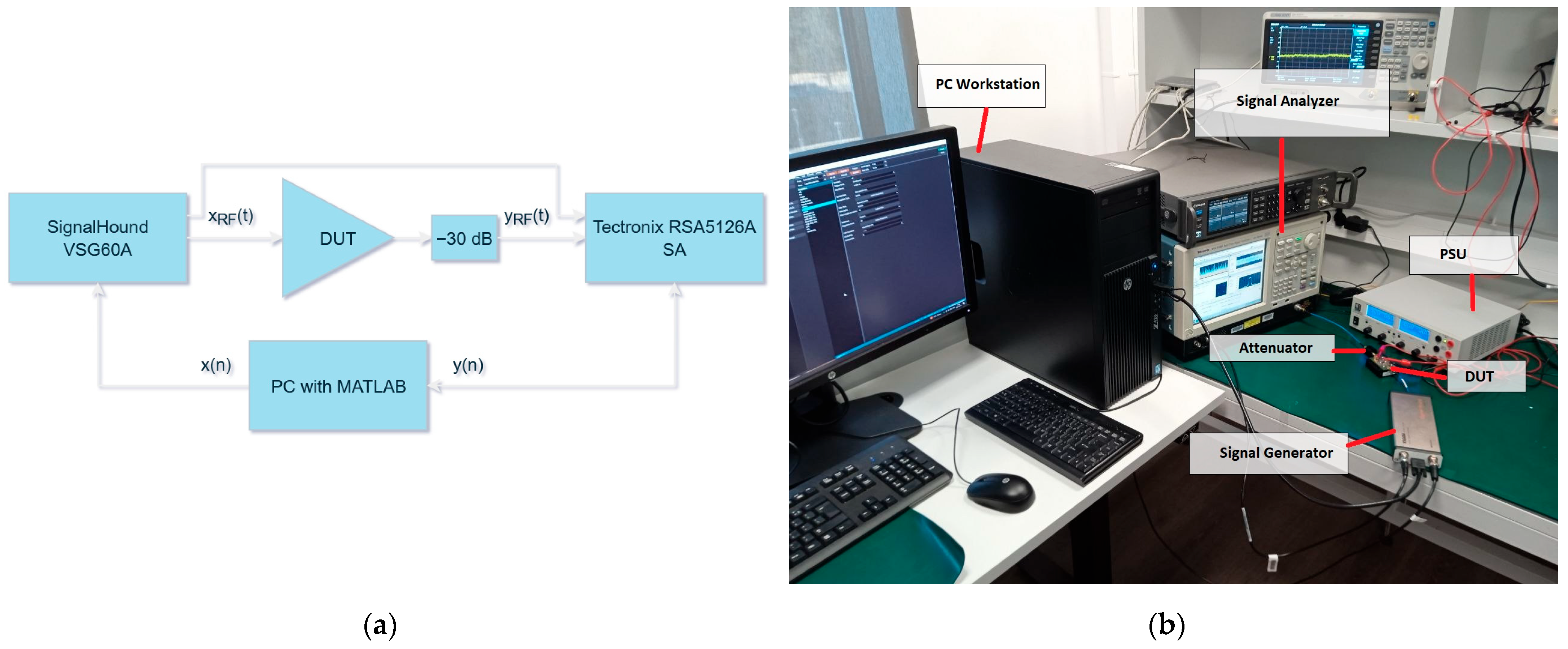
The proposed parametric MP model was validated using the measurement setup illustrated in Figure 1 (power supply and synchronization cables were omitted for clarity). The setup consisted of a vector signal generator (VSG) and a signal analyzer (SA). In addition to the primary signal path through the device under test (DUT), a reference path was included. The DUT was a QPA9942 power amplifier with an operational frequency range of 3300–3800 MHz, which is used in wireless communication in TDD mode using channel bandwidths down to units of megahertz. A SignalHound VSG60A was used for signal generation, and a Tektronix RSA5106A was used for signal analysis. Both instruments were controlled by a PC running MATLAB 2024b software. For a predefined baseband excitation signal x, a series of measurements was conducted by sweeping the carrier frequency of x_RF(t). The direct signal path from the VSG to the SA enables the comparison of the baseband equivalents of x_RF(t) and y_RF(t), thereby facilitating a direct input-to-output characterization of the DUT.

The measurement was designed to cover the entire 3.3–3.8 GHz operational bandwidth of the QPA9942 amplifier. A frequency step of 10 MHz was selected, resulting in a total of 51 distinct carrier frequencies and corresponding datasets. Each recorded input and output waveform comprised 32,768 samples. The excitation signal featured a 1 MHz modulation bandwidth and was captured at a receiver sample rate of 8 MHz.

The average output power ranged from approximately 28 to 31 dBm across all datasets; this variation is attributed to the amplifier’s non-flat frequency response, which produces different gain values at different frequencies. This power level was selected as optimal for the device’s power-added efficiency (PAE), as specified by the manufacturer, and is sufficiently high to drive the amplifier near its saturation region. The excitation signal had a peak-to-average power ratio (PAPR) of approximately 6.5 dB.

To determine the optimal model complexity, a grid search was conducted to evaluate the NMSE across various polynomial degrees (K) and memory depths (M). Figure 2 depicts the results of this search for two frequencies, 3.3 GHz and 3.8 GHz.

Figure 2 reveals that the optimal model order is frequency-dependent, and a memory depth of M = 2 is required at 3.3 GHz to capture significant memory effects. A memory depth of M = 1 suffices at 3.8 GHz, indicating quasi-static operation. A fixed structure (K = 5, M = 2) was selected as it represents the lowest common order that minimizes error across both frequencies. This results in a standard MP model with 10 coefficients and a parametric MP model requiring 10 continuous functions, $p_{km}\left(f_c\right)$.

The implementation of the parametric MP in Equation (3) involves two critical design considerations: First, the number of interpolated anchor points and their distribution across the frequency axis. The first aspect is conceptually straightforward; a higher number of points generally yields a more accurate approximation of the underlying coefficient functions. However, this improved accuracy comes at the cost of increased measurement overhead and greater computational complexity. To balance this trade-off, this paper evaluated PMP performance across several approximation orders (i.e., different numbers of points). Second, the optimal distribution of these selected points along the frequency band is considered. While a uniform (linear) distribution is the most intuitive starting point, its performance can be compared against more sophisticated sampling strategies. Specifically, this work will contrast the results from a uniform distribution with those achieved using a Chebyshev node distribution, which is designed to minimize interpolation error by concentrating points near the boundaries of the interval.

3. Results

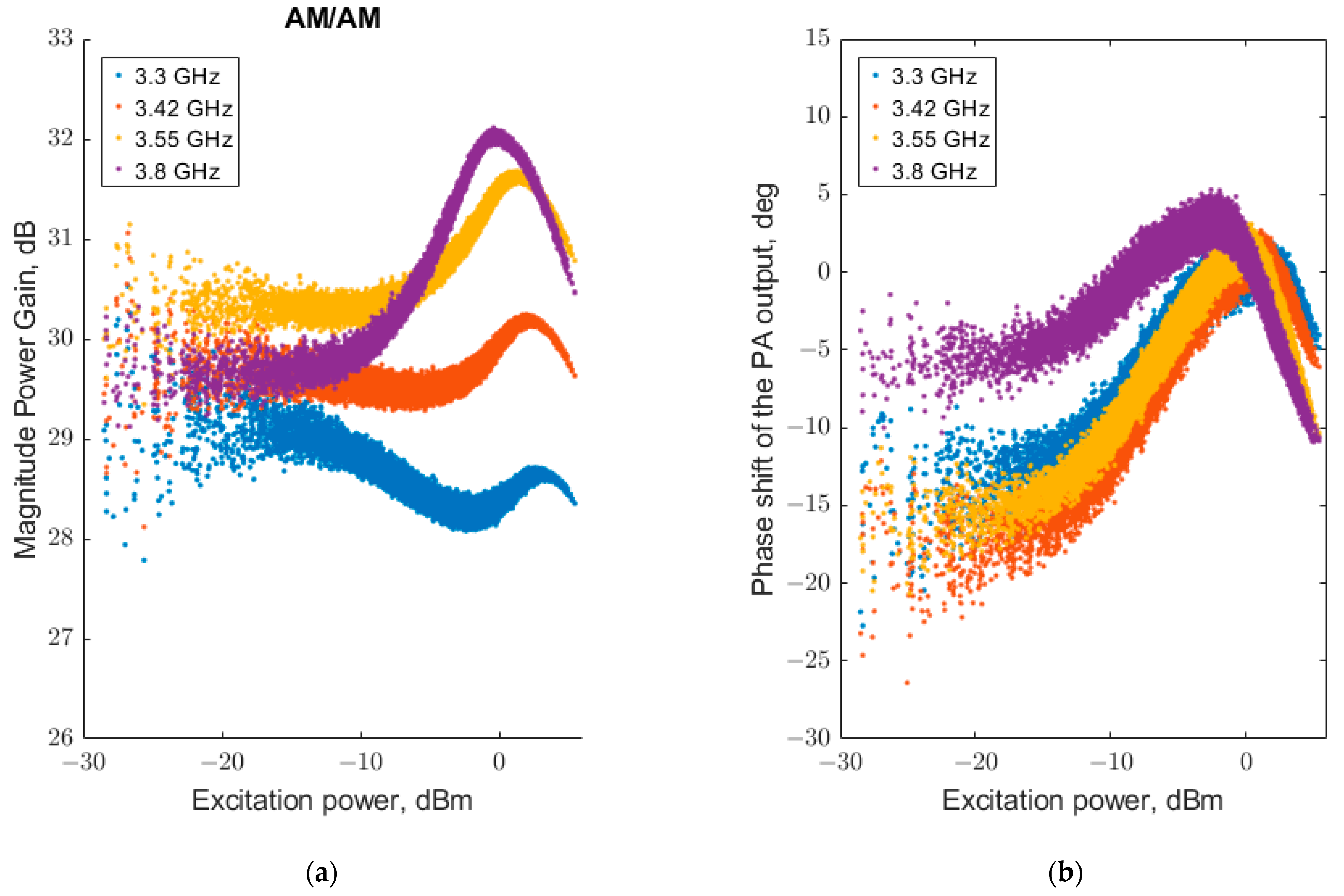
Figure 3 presents the AM/AM and AM/PM characteristics of the PA measured at four distinct carrier frequencies. The results demonstrate that the PA‘s behavior is significantly influenced by the carrier frequency. This dependence affects not only the signal gain but also the phase relationship, a phenomenon likely attributable to the frequency-sensitive parasitic inductances and capacitances inherent to the PA’s architecture.

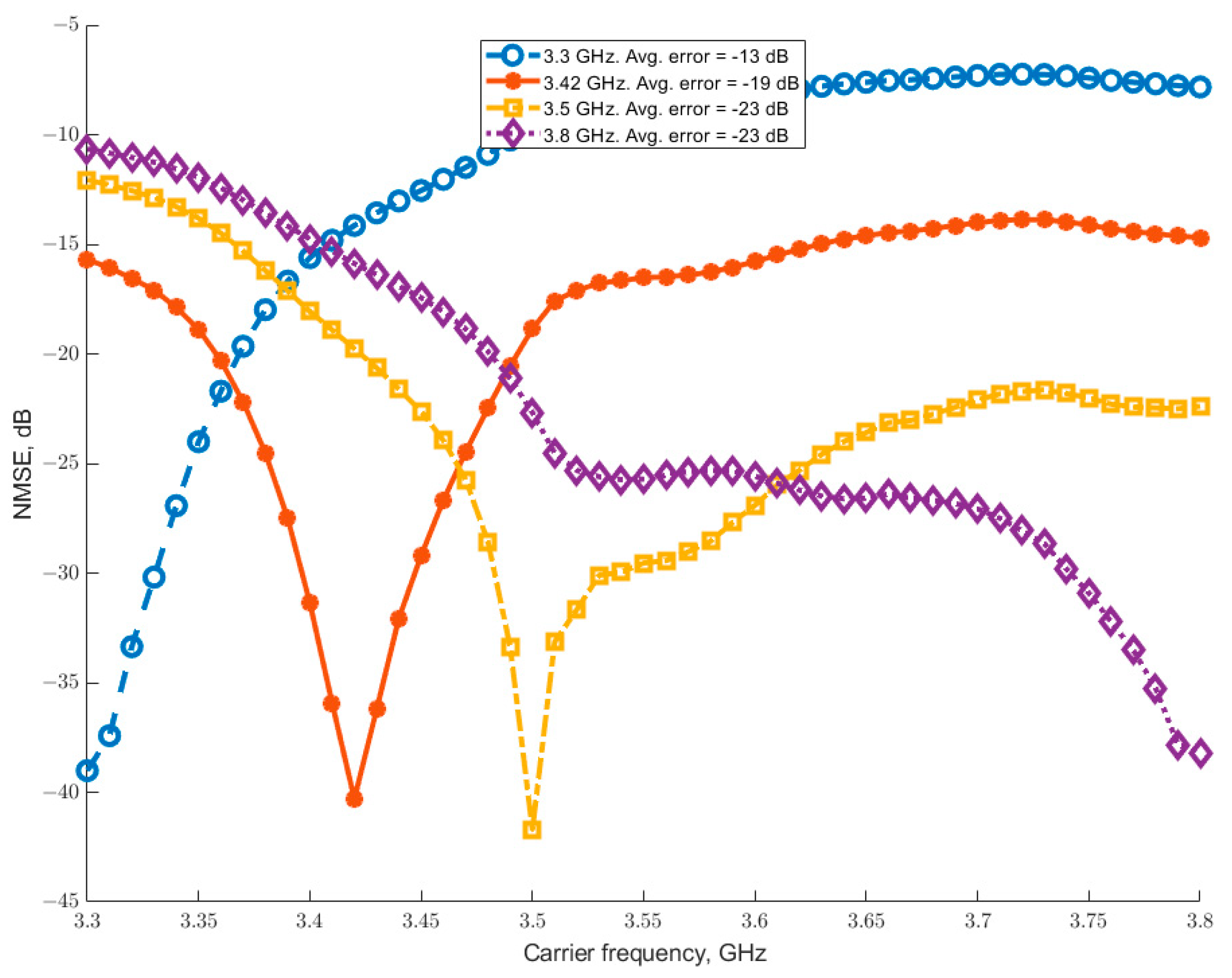
To establish a performance baseline for comparison with the proposed PMP model, a standard MP model was extracted from a dataset at a single frequency. This model was then applied to data from different frequencies. The results of this baseline experiment, presented in Figure 4 for the same four frequencies as in Figure 3, reveal two findings as follows: First, the baseline modeling error at the model extraction point varies with frequency. Second, a clear and systematic increase in error is observed as the carrier frequency of the application data diverges from the extraction frequency.

For a quantitative assessment of model performance across the frequency band, the average NMSE was computed for each test case:

$$e_{avg}={\displaystyle \frac{1}{51}}\sum _{f_c=1}^{51}{e}_{dB}\left(f_c\right).$$

(9)

The resulting average error values for each single-frequency model are displayed in Figure 4. The analysis reveals that the model extracted at 3.3 GHz yields the largest average error across the band, while the model from 3.55 GHz yields the smallest error. This indicates that a single model extracted at 3.55 GHz performs, on average, approximately 11 dB better over the entire operational bandwidth than one extracted at 3.3 GHz.

A comparison of these modeling results with the transfer characteristics in Figure 3 elucidates the reason for this discrepancy. The AM/AM characteristic at 3.3 GHz exhibits a significantly lower average gain and a different shape compared to the response at 3.55 GHz. This suggests that the behavioral characteristics of the PA at 3.55 GHz are more representative of its average behavior across the operational bandwidth. Consequently, the 3.55 GHz response is selected as the baseline for subsequent comparison.

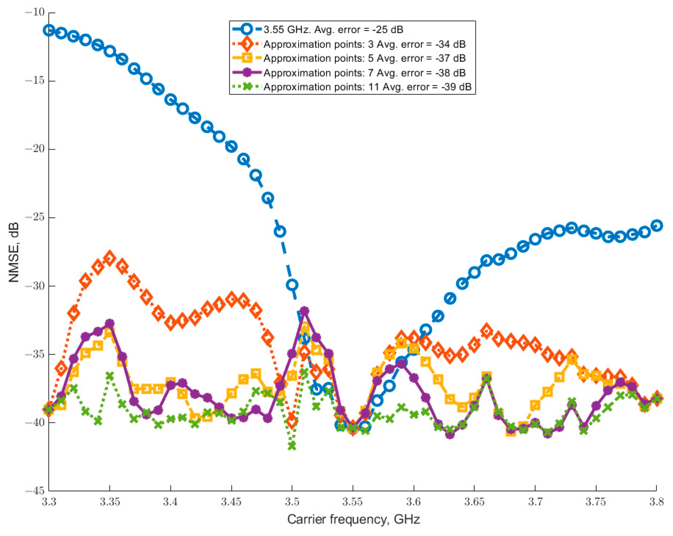
Figure 5 presents a performance comparison between the baseline single-frequency model and four PMP models. The PMP models were constructed using 3, 5, 7, and 11 interpolation points, distributed uniformly across the 3.3–3.8 GHz frequency range (with each point rounded to the nearest measured frequency value).

The results demonstrate a notable reduction in modeling error across the entire carrier-frequency band compared to the baseline. The PMP model derived from 3 points achieves an average error reduction of approximately 9 dB. Increasing the interpolation order to 5 and 7 points yields further improvements, reducing the average error by 12 dB and 14 dB, respectively, relative to the baseline.

To evaluate the impact of node distribution on modeling accuracy, the interpolation points were also allocated according to the Chebyshev node distribution. For the frequency range of 3.3–3.8 GHz, which is represented by measurement indices 1 through 51, the k-th node index (for k = 0, 1, … N), is given by the formula:

$$f_k= round\left({\displaystyle \frac{51-1}{2}}\mathit{cos}\left({\displaystyle \frac{2N+1-2k}{2\left(N+1\right)}}\pi \right)+{\displaystyle \frac{1+51}{2}}\right).$$

(10)

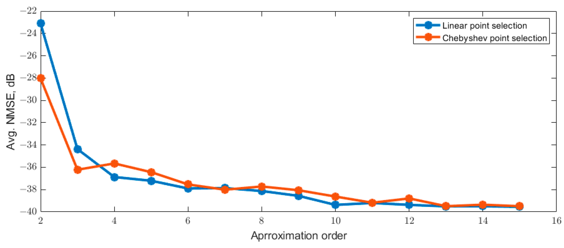
This distribution yields a higher density of nodes near the boundaries of the interpolation interval. Figure 6 compares the average NMSE achieved using a uniform (linear) point distribution against that of the Chebyshev distribution. The results demonstrate similar performance trends for both methods. The Chebyshev distribution exhibits a minor disadvantage at higher approximation orders (e.g., >7 points) but a slight advantage at low orders (2–3 points). This finding indicates that the specific selection of interpolation points has a negligible impact on the overall modeling error, provided the points are sampled across the entire operational bandwidth and a spline interpolation technique is employed.

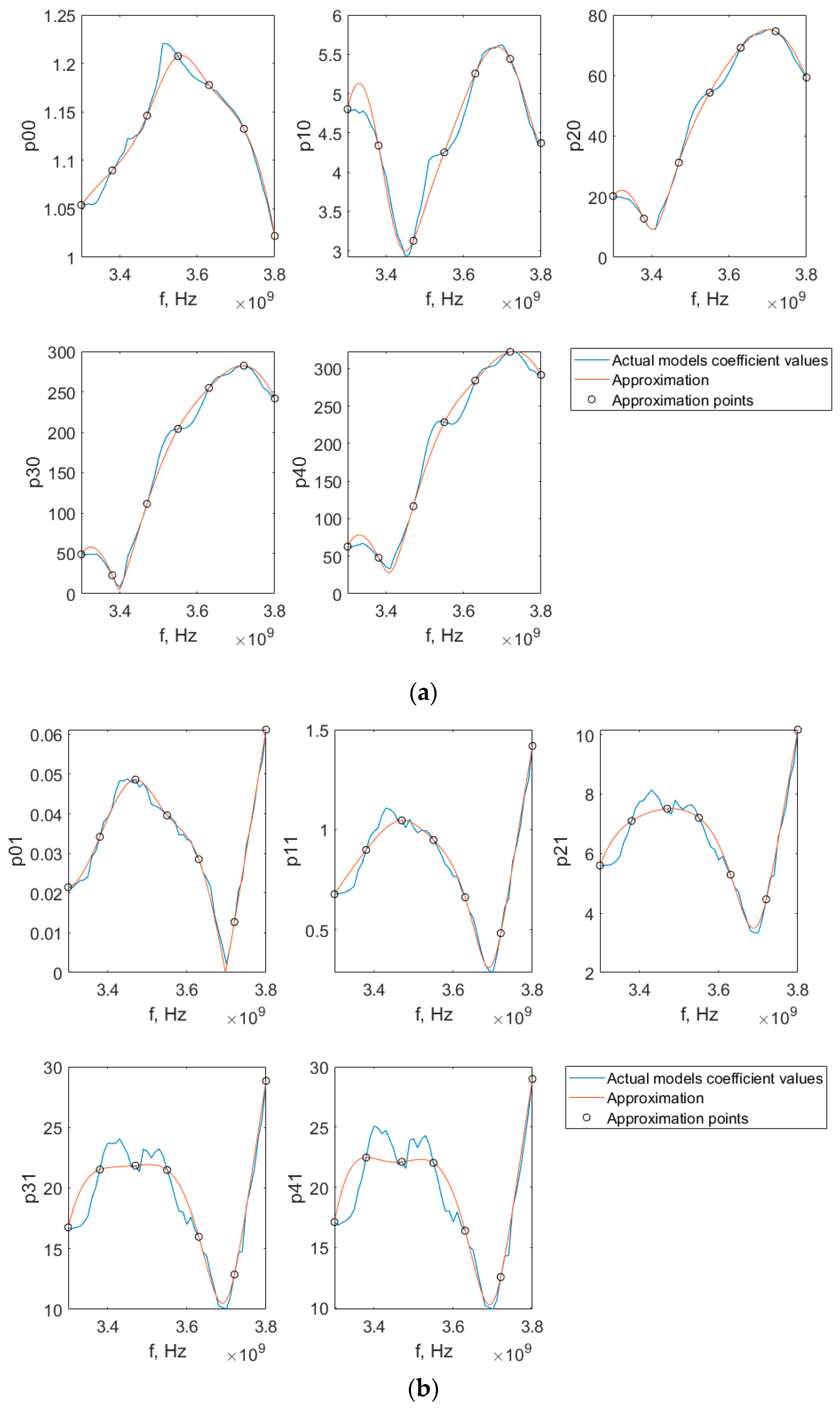
Figure 6 also reveals a saturation effect in the modeling error, where its sensitivity to increases in approximation order diminishes. This phenomenon can be explained by examining the frequency-dependent behavior of the MP model coefficients, as illustrated in Figure 7, as well as initial model fitting accuracy across the band. Figure 7 shows the 10 continuous functions, p_km(f), derived using 7 interpolation points, against the discrete coefficient values a_km,b_km…c_km obtained from extracting standard MP models from all 51 individual datasets.

A visual analysis shows that the coefficients associated with the first memory tap (m = 0) are accurately captured by the smooth interpolating functions. In contrast, the coefficients of the second memory tap (m = 1) exhibit a poor fit. This discrepancy arises because the underlying values of these higher-order coefficients demonstrate a more erratic, non-smooth dependence on frequency. The root cause of the non-smooth behavior observed is difficult to isolate. However, the most plausible explanation aligns with the phenomenon illustrated in Figure 2: the power amplifier exhibits different behavioral regimes at different carrier frequencies. Specifically, certain frequencies show noticeable memory effects, while at others, the PA operates in a quasi-static manner.

This frequency-dependent shift in dynamics presents a challenge for a fixed-model structure. The standard memory polynomial model, with its predetermined memory depth, is applied uniformly across all frequencies. Consequently, at frequencies where memory effects are pronounced, the second tap coefficients accurately capture real physical behavior. In contrast, at frequencies where the PA response is essentially static, these same coefficients lack a strong underlying physical correlation. Without sufficient excitation for these terms, the LSE process produces unstable and noisy solutions, manifesting as the observed non-smooth trajectories in the coefficient curves.

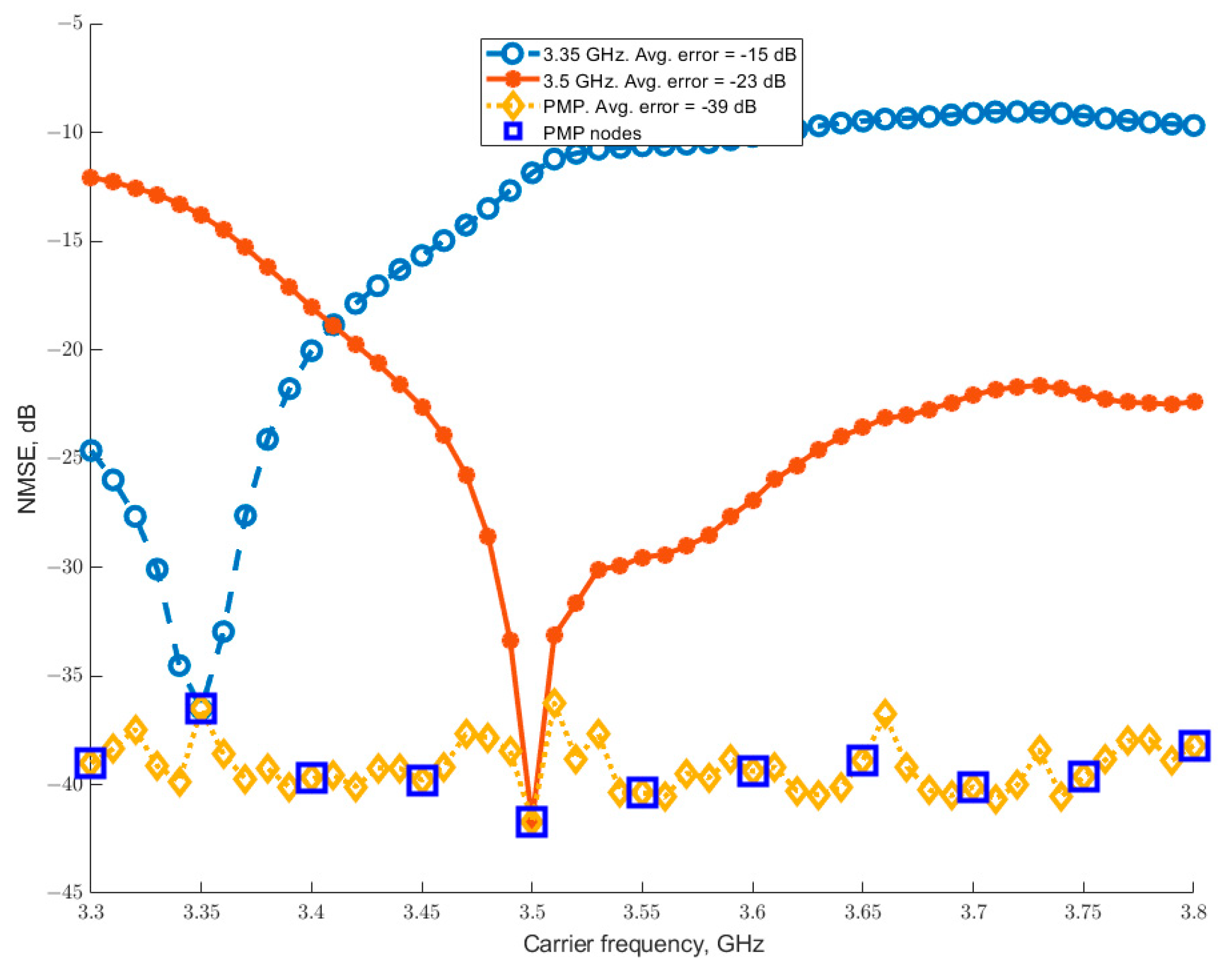
The limitation of employing a fixed model structure is further illustrated in Figure 8, which depicts the performance of the PMP model trained on 11 nodes (marked by blue squares). The resulting model exhibits an oscillatory error across the frequency band. This oscillation is a direct consequence of the inherent variation in the accuracy of the underlying single-frequency MP models used for training.

As evidenced in the figure, the initial MP models demonstrate different levels of performance at their respective extraction frequencies; for instance, the model at 3.5 GHz achieves an NMSE of –41.7 dB, while the model at 3.35 GHz only achieves –36.5 dB. Since the parametric model is derived from these discrete points, their residual errors become anchor points that the PMP must interpolate, thereby propagating the initial inaccuracies into the continuous frequency-dependent function. This performance discrepancy arises because the chosen fixed model structure (K = 5, M = 2) is inherently better suited to characterizing the PA’s behavior at some frequencies (e.g., 3.5 GHz) than at others (e.g., 3.35 GHz).

The saturation effect observed in Figure 6 is also attributable to the fitting errors of the initial single-frequency MP models. The mean NMSE of the 11 anchor points used for training, as shown in Figure 8, is –39.4 dB. This value aligns closely with the asymptotic limit of the PMP’s performance in Figure 6. This result is conceptually intuitive: the parametrization process cannot surpass the average accuracy of the models upon which it is based, as it operates solely on their coefficients rather than on the original measurement data. The PMP’s performance is, therefore, fundamentally bounded by the quality of the initial MP estimations.

Given that the accuracy of the proposed PMP model is contingent upon both the initial single-frequency MP model fitting accuracy and the error introduced by spline interpolation, it is instructive to analyze the contribution of each component separately.

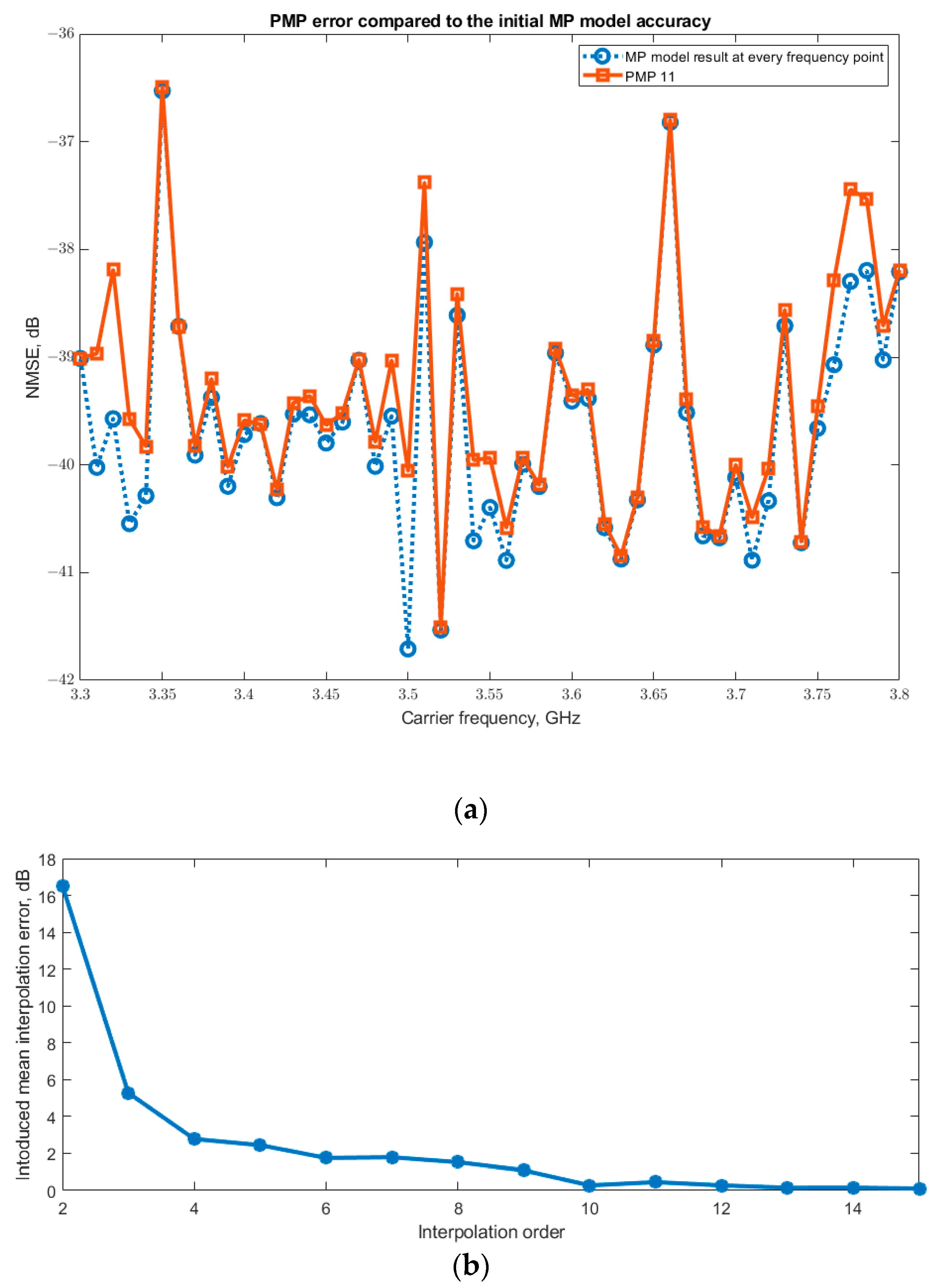
Figure 9a illustrates this relationship by comparing the performance of the 11th-order PMP model against the fitting error of all initial MP models. The initial fitting error (represented by the blue line) was determined by evaluating each of the 51 standard MP models exclusively at their own extraction frequency. As expected, the PMP error curve intersects these points precisely at the anchor frequencies and exceeds them in the intervening regions, demonstrating the additive effect of interpolation error.

To isolate the interpolation error, Figure 9b shows the difference between the PMP error and the initial MP fitting error for approximation orders ranging from 2 to 15. This analysis reveals that the interpolation error component diminishes rapidly and approaches zero as the approximation order reaches 10. This indicates that for orders ≥10, the overall PMP error is dominated almost entirely by the initial MP fitting inaccuracy, confirming that the interpolation itself becomes nearly ideal with a sufficient density of anchor points.

4. Discussion

The standard MP model extracted at 3.55 GHz achieves an NMSE of approximately –40.4 dB at its extraction frequency. As illustrated in Figure 6, the PMP model derived from ten frequencies nearly replicates this level of performance across the entire 3.3–3.8 GHz band, significantly improving frequency generalization. However, the result is not ideal, as evidenced by the oscillation in the NMSE curve. This oscillation is in part caused by the coefficient interpolation error, as shown in Figure 7b. The second part of this oscillation is directly attributable to the inherent discrepancy in the fitting accuracy of the initial single-frequency MP models across the operational band, as demonstrated by the varying error levels at the anchor points in Figure 8. The parametric model’s ability to generalize is fundamentally constrained by the quality and consistency of these underlying local approximations.

This irregularity in the coefficient trajectories may suggest that the memory effects were not uniformly or sufficiently excited across the entire measurement bandwidth. This insufficient excitation could lead to instability and fluctuations in the LSE solution used for coefficient extraction. As initially demonstrated in Figure 2, the DUT exhibits both dynamic and quasi-static behavior under the identical excitation signal, depending on the carrier frequency. This mixed dynamic and quasi-static behavior poses a challenge for frequency-adaptive modeling, as the same excitation may activate different nonlinear mechanisms at different frequencies. Had the PA’s behavior been consistently dynamic or consistently quasi-static across the band, the irregular, non-smooth nature of the coefficient curves would likely be far less severe or even non-existent. Furthermore, a more consistent behavioral response from the power amplifier across the operational frequency band would likely lead to a more uniform accuracy among the initial single-frequency MP models. This uniformity would, in turn, provide a more stable foundation for the parametric interpolation, likely enhancing the overall performance and predictive capability of the PMP model by eliminating the erratic coefficient behavior caused by the current performance discrepancies. As demonstrated in Figure 9, the interpolation error introduced by the parametric method effectively diminishes to a negligible level once the approximation order reaches ten. Beyond this point, the overall error of the PMP model is dominated solely by the inherent inaccuracy of the initial single-frequency MP models. These discrepancies in the initial model fitting are a direct consequence of the fundamental variance in the power amplifier’s behavioral characteristics across the operational frequency band. Consequently, any further significant improvement in the overall PMP accuracy must be achieved by reducing this initial modeling discrepancy, rather than by increasing the interpolation order.

An important assumption underlying the proposed parametrization technique is that the power amplifier exhibits reasonably smooth behavioral characteristics across its operational bandwidth. This assumption of continuity validates the use of a uniform (linear) node distribution, as it minimizes the risk of missing significant nonlinear irregularities between the interpolation points. However, should the PA’s response contain sharp discontinuities—such as narrowband resonance peaks or valleys within the operational band—this approach would be insufficient. In such scenarios, accurately capturing the PA’s behavior would necessitate a substantially denser distribution of frequency nodes. Alternatively, an optimal sampling strategy would require prior knowledge of the irregularity locations to place interpolation points strategically and ensure they are adequately captured by the model.

Considering the real-time deployment of the model, the proposed PMP modeling approach introduces a moderate increase in computational overhead during an offline training stage, while maintaining minimal runtime cost during deployment. Specifically, the training stage requires extracting N memory polynomial models, each using M input-output samples and producing P coefficients. This involves solving N least-squares regression problems, each with a computational complexity of $O(M{P}^2+P^3),$ resulting in an overall cost of $O(NM{P}^2+N{P}^3)$. Once the MP models are obtained, spline interpolation is performed for each of the P coefficients across the N frequency points to obtain frequency-dependent coefficient functions. For the calculation of the splines, this step is computationally efficient, with a total complexity of $O\left(PN\right)$, and it is performed only once. During online operation, the model requires evaluating these P spline functions at the current carrier frequency, which involves evaluating a cubic polynomial per coefficient and has negligible overhead $O\left(P\right)$. Therefore, the added computational cost of the proposed PMP technique is confined to the offline training phase, while its runtime complexity remains comparable to that of a standard memory polynomial model, allowing for possible integration into real-time digital predistortion systems.

The proposed parametric MP model is particularly suited for practical deployment in Low-Power Wide-Area (LPWA) networks, such as NB-IoT and LoRaWAN. These applications are characterized by their use of lower bandwidth transmissions and a critical requirement for long-range, energy-efficient communication. Devices in these networks must often operate across multiple fragmented frequency bands to connect to different gateways or adhere to regional regulations. The PMP’s ability to provide a single, pre-trained model that generalizes across a wide frequency range—without the need for retraining or a bank of models—directly addresses this need for frequency agility.

While the proposed PMP model demonstrates an advancement in frequency-agile behavioral modeling, its performance is ultimately bounded by the accuracy and consistency of the underlying single-frequency models upon which it is built. The technique’s efficacy can be diminished by impedance mismatches or insufficient memory effect excitation, which challenge the core assumption of coefficient smoothness. Despite these limitations, the PMP framework provides a foundation for real-time linearization across bandwidths where traditional models fail. Its performance in controlled experiments presents a promising path toward practical adaptive digital predistortion systems for modern wireless applications, particularly in low-power wide-area networks where frequency agility is paramount. Future work will focus on integrating adaptive model structures to overcome the current constraints and further enhance generalization capabilities.

5. Conclusions

This paper presents a parameterized memory polynomial model capable of generalizing power amplifier behavior across a wide carrier-frequency range. Unlike the conventional MP model, which performs poorly outside of its extraction frequency, the proposed method captures the frequency-dependent variation of model coefficients using interpolation techniques, significantly reducing modeling error across the band. Experimental results demonstrate that even sparse frequency sampling (e.g., 3 points) offers substantial accuracy gains up to 9 dB average NMSE improvement. The model achieves near-optimal performance over the full 3.3–3.8 GHz band, closely approaching the accuracy of individually tuned models while maintaining moderate computational costs for the training phase. This work demonstrates that the performance of a frequency-parameterized model is fundamentally bounded by the accuracy of the initial single-frequency models from which it is derived. The observed saturation in modeling improvement and the residual oscillatory error are direct consequences of the inherent discrepancy in these initial MP model accuracies across the band. Consequently, achieving optimal generalization requires not only an effective parametrization technique but also a consistent foundational model at each anchor frequency. Future work will, therefore, focus on adaptive model structures that can accommodate the PA’s varying behavioral regimes to minimize this initial error discrepancy.