Article

Adaptive Optimization of Traffic Sensor Locations Under Uncertainty Using Flow-Constrained Inference

1
Civil Engineering Department, Faculty of Engineering, Assiut University, Assiut 71515, Egypt
2
Civil Engineering Department, Faculty of Engineering, Sphinx University, New Assiut 71515, Egypt
3
Mathematics Department, Faculty of Science, Assiut University, Assiut 71515, Egypt
4
Basic Science Department, Faculty of Engineering, Sphinx University, New Assiut 71515, Egypt
*
Author to whom correspondence should be addressed.
Appl. Sci. 2025, 15(18), 10257; https://doi.org/10.3390/app151810257
Submission received: 4 September 2025 / Revised: 16 September 2025 / Accepted: 16 September 2025 / Published: 20 September 2025
(This article belongs to the Section Transportation and Future Mobility)

Abstract

Monitoring traffic flow across large-scale transportation networks is essential for effective traffic management, yet comprehensive sensor deployment is often infeasible due to financial and practical constraints. The traffic sensor location problem (TSLP) aims to determine the minimal set of sensor placements needed to achieve full link flow observability. Existing solutions primarily rely on algebraic or optimization-based approaches, but often neglect the impact of sensor measurement errors and struggle with scalability in large, complex networks. This study proposes a new scalable and robust methodology for solving the TSLP under uncertainty, incorporating a formulation that explicitly models the propagation of measurement errors in sensor data. Two nonlinear integer optimization models, Min-Max and Min-Sum, are developed to minimize the inference error across the network. To solve these models efficiently, we introduce the BBA Algorithm (BBA) as an adaptive metaheuristic optimizer, not as a subject of comparative study, but as an enabler of scalability within the proposed framework. The methodology integrates LU decomposition for efficient matrix inversion and employs a node-based flow inference technique that ensures observability without requiring full path enumeration. Tested on benchmark and real-world networks (e.g., fishbone, Sioux Falls, Barcelona), the proposed framework demonstrates strong performance in minimizing error and maintaining scalability, highlighting its practical applicability for resilient traffic monitoring system design.

1. Introduction

A transportation network’s link (street/edge/arc) flow provides understandable information for monitoring the overall network’s traffic state and may be utilized to improve traffic management and control. However, a network-wide traffic sensor system may not be feasible for practical applications. Large or moderate-sized metropolitan networks need the deployment of many sensors, which can be costly. This emphasizes the importance of addressing the problem of optimal sensor locations within a limited budget, identifying a minimum subset of links and their locations, so that the objective of monitoring the network is achieved efficiently. Interestingly, TSLP has become a problem that is simple to define but complex to solve. The TSLP search space, with ( 2 n 1 ) possibilities, may be considered a single-sided illustration of its complexity, where m is the number of network edges, and 2 is the binary selection for each link/node. Setting the number of deployed sensors to l reduces the search space domain to
S ( m , ) = m = m ! ! ( m ) !
where, m is the number of candidate locations and is the number of sensors. S ( m , ) represents the search domain function for n and m and counts how many ways we can choose out of m (the binomial coefficient). However, this decrease remains large for moderate-sized networks [1]. The sensor placement problem is inherently combinatorial, involving the selection of a subset of candidate locations to optimize network observability. Studies have demonstrated that this problem exhibits submodular characteristics, allowing for efficient optimization strategies [2,3]. Additionally, Ref. [4] explored the combinatorial aspects of sensor location, providing insights into the complexity and potential solutions for optimizing sensor deployment.
Most TSLP formulations in the literature are proven to be NP-hard [5,6]. Therefore, the traffic sensor location problem (TSLP) gained significant attention in the transportation research sector. The seminal work of [7] classified the TSLP objectives into six main categories, namely flow observability, O/D updating/estimation [8,9], link flow inference [10,11], travel time estimation [12], screen line/traffic surveillance [13,14], and path reconstruction [15] problems. This delicate classification system aims to clarify the nuanced differences among the numerous TLSP studies in the literature. Many researchers [4,16,17,18,19,20] have placed a high value on the flow observability problem, which is also the focus of this study’s research. Flow observation systems are usually intended to use flow conservation equations to gain information about the unseen flows [21,22]. Sensor failures/errors in such systems may result in a loss of flow information for both seen and inferred linkages [23]. The flow observability challenge tackles all network flow components (e.g., O/D, link, and route flows), with the goal of estimating all flow values by directly measuring a subset. In recent years, increasing attention has been given to the traffic sensor location problem under uncertainty, with several studies proposing advanced formulations and solution approaches. For instance, observability-based methods have been explored to enhance the theoretical foundation of sensor placement strategies [24]. Robust optimization models have also been introduced to explicitly account for measurement uncertainties and improve the reliability of traffic state estimation [25]. In addition, efficient metaheuristic techniques have been applied to scale the problem to large and complex transportation networks, demonstrating the practicality of such approaches in real-world applications [26]. These contributions highlight the growing relevance of the problem and further justify the need for scalable and robust methods, as developed in this study.
The initial step in TSLP flow observability is to define a system of linear equations. The system shows the interaction between various flow parts, with connections formed from flow propagation rules in a network based on expected user route-choice behavior. In this regard, the TSLP seeks to identify the smallest set of observed O/D, link, or route flows that traffic sensors can monitor in order to find a solution to the formulated equations. The remaining non-observed/measured flow components may be answered in either whole or partial contexts. In the TSLP literature, several foundational assumptions are frequently made to guide the direction of research. These assumptions typically include the type of sensor under investigation, sensor locations within the network elements (i.e., node or link), budget constraints, and the uncertain nature of sensor data. In practical applications, various monitoring technologies are utilized, such as inductive loops, weight-in-motion sensors (using piezoelectric or quartz technology), image recognition (video systems), laser sensors, and multi-technology systems that combine laser, radar, and ultrasonic sensors.
TSLP studies often categorize sensing technologies into active and passive sensors. In passive-mode scenarios, only edge flows are counted, whereas active sensors require additional information, including vehicle type, route details, and observation time [27,28]. Therefore, it is essential for TSLP research to clarify whether the sensing mode is passive, active, or heterogeneous (a combination of both). Traffic flow information is typically divided into three categories: O/D (origin/destination) demand, link flow, and route flow. Traffic-flow propagation models are structured in a hierarchy, but one of their biggest challenges is that traffic flows are not always easy to observe directly. For instance, link flows—those that occur along specific roads—can be tracked using passive sensors installed on selected streets. Path flows, on the other hand, need either path-ID sensors or active sensors that estimate them indirectly. The most difficult to observe are origin-destination (O/D) flows, which most sensor types cannot capture at all. This makes it crucial to carefully consider where sensors are placed and what types are used. For example, at network junctions, you need sensors that can measure how vehicles split and turn, along with total vehicle counts.
A major obstacle in Traffic State and Load Prediction (TSLP) is the limited number of sensors that can be installed—usually because of budget constraints. To get around this, researchers have turned to mathematical models and statistical techniques based on how traffic naturally propagates through the network. Even with fewer sensors, these TSLP methods have been quite successful in extracting meaningful traffic data [29,30,31]. Still, there is a key assumption that often goes unchallenged: that sensors always provide perfect, error-free data. In practice, though, this is rarely the case. Sensor data can be uncertain due to things like measurement errors or even full-on sensor failures. Unfortunately, only a few studies have looked into how these issues impact the overall system. Errors in measurement can ripple through the whole process, leading to misleading results [32]. Conversely, sensor failure can result in the loss of vital flow information, which undermines the accuracy of traffic monitoring [17]. Recent research has aimed to mitigate the effects of such errors by accounting for error variations in the system or minimizing the impact of sensor failure probabilities [23]. To this end, few studies, only two [20,32], have tackled error propagation while solving the TSLP for the link observability problem. This study addresses the problem specifically by dealing with the errors and uncertainties inherent in sensor data. Scalability is the main concern of the developed solution methodology, where advanced metaheuristics are adapted for the first time to the formulated TSLP. By incorporating error management strategies, the reliability of traffic flow data would be enhanced, ultimately leading to more accurate traffic monitoring and better-informed decisions in network management. The remainder of this article is organized as follows. Section 2 surveys the state of the art and framework of the traffic sensor location problem (TSLP) and the main contribution. Section 3 formulates the problem, notation, and assumptions. Section 4 analyzes the complexity of the problem and the key theoretical properties. Section 5 details the proposed methodology. Section 6 presents case studies and numerical experiments. Finally, Section 7 concludes the paper and outlines the directions for future work.

2. State of the Art

In general, the literature on the traffic sensor location problem (TSLP) is extensive and well-developed. Comprehensive and up-to-date evaluations of the sensor placement problem have been provided by researchers such as [1,5,6,7,33]. In this section, our focus is specifically on the TSLP in the context of link flow observability, with particular attention to challenges posed by uncertainty, including sensor failures, measurement inaccuracies, and incomplete traffic information.

2.1. TSLP for the Observability Problem

The link flow observability challenge is to determine the smallest number of sensors and their positions on the network such that the measurements obtained by installed sensors enable the complete determination of flows on all unseen arcs [34]. The smallest number of sensors results in the lowest maintenance and installation costs, while their best positions enable complete link flow observability, which means that all unseen link flows may be inferred from observed flows [35]. As a result, the essence of the TSLP for the link flow observability problem is to identify the optimal location of sensors on the network based on flow conservation, allowing for the unique determination of the solution of the linear system of equations associated with the sensors.
Castillo, in collaboration with multiple co-authors, has made substantial contributions to studying the observability problem through a series of rigorous and methodologically diverse investigations. Ref. [36] utilized the mathematical definition of the observability issue as a linear system of equations to determine if the existing flow measurements were adequate to solve the system’s state. Ref. [37] suggested a polynomial solution approach based on sequential Gaussian eliminations to obtain the necessary sensor readings for global network observability. This may be seen as a modified topological version of the previous algebraic technique. Alternatively, Ref. [35] created a complete matrix tool to handle this issue, which contains all flow components as binary variables. Ref. [34] then developed an approach for determining the maximum number of sensors necessary to solve the challenge. Ref. [38] tackled the TTSLP problem using plate-scanning sensors, combining matrix-based techniques with pivoting algorithms to enhance flow estimation.
Earlier, a foundational study by [16] introduced a linear-algebra-based approach that relied on the link-path incidence matrix. They developed what is known as the “basis link” method, designed specifically for steady-state traffic conditions. The core idea was to represent the network structure using the incidence matrix, then identify a subset of key links—called basis links—such that, if sensors are placed on them, the traffic flows on all other links can be inferred using linear combinations. This was achieved through the reduced row echelon form of the matrix, a classic tool in linear algebra. Notably, their method does not require any prior knowledge of origin–destination (O/D) flows or traffic assignment models, which makes it particularly practical for real-world networks where such information is often missing or difficult to obtain. They tested their method on a range of network types, from basic layouts like fishbone structures to more complex examples like the Sioux Falls network, which includes 182 O/D pairs and 76 links. Even at this scale, the basis link method proved efficient in identifying the minimal number of sensor-equipped links needed for full flow estimation. Results showed that in large-scale networks, up to 81% of the links required sensors, though this percentage varied depending on the network’s topology and the number of available paths. The method also accounts for network connectivity, indicating that more connected networks require fewer sensors, thus providing a cost-effective solution. Additionally, sensitivity analyses showed that the optimal sensor placement is highly dependent on network topology, with an upper bound on the number of basis links dictated by the network structure itself. While the method is effective for small-scale problems, this method struggles with large-scale networks due to computational limits related to full path enumeration. Alternatively, Ref. [39] introduced a node-based approach for solving the TSLP without relying on path enumeration, which can be computationally expensive for large-scale networks. The formulation focuses on minimizing sensors number for the observability problem by leveraging the node–link incidence matrix. This elimination of full path enumeration, which traditionally made the problem intractable for larger networks, involves linear flow conservation at non-centroid nodes. The method is based on synergistic sensor placement, where one sensor’s placement impacts others’ placement. The tested networks showed that only about 60% to 70% of the links needed to be equipped with sensors to achieve full link flow observability. Also, the Sioux Falls network is the largest network solved in the study. Ref. [10] extended the previous work by tackling the partial link flow observability problem in networks where some sensors had already been deployed. The partial observability issue addresses the minimization of unobserved link numbers or overall flow information loss while working with a restricted sensor budget. The study aims to determine the minimum number of additional sensors needed to complete flow observability, given that some link flows are already known. The node–link incidence matrix is once again used for formulating the problem, and the solution is based on synergistic sensor placement, where the deployment of one sensor aids in observing other flows. The approach focuses on partial observability and the interaction between initial sensor placements and subsequent sensor requirements. The study tested the methodology again on the Sioux Falls network. The results showed that around 45% of the network links needed to be equipped with sensors to achieve partial observability. Ref. [40] used a graphical approach (i.e., spanning tree approach) to solve the TSLP. The largest network tested in the study consisted of the Sioux Falls network, where the results showed that approximately 55% of the network’s links are needed for full coverage. Ref. [41] tackled the TSLP by introducing two different methods: an exact branch-and-bound (B&B) algorithm and a genetic algorithm (GA). While the B&B algorithm guarantees finding the optimal solution, it comes with a heavy computational cost, making it less practical for larger networks. In contrast, the genetic algorithm offers near-optimal solutions much more efficiently, which makes it better suited for bigger networks. In their experiments, the largest network tested was a grid with 150 links. They found that the GA needed sensors on only about 60% of the links to ensure full observability, whereas the B&B approach was limited to networks with fewer than 100 links due to its longer computation times.
More recently, Ref. [21] introduced a new mathematical factorization approach using LU decomposition to analyze link flow observability in transportation networks. Their method reformulates the traditional traffic assignment problem into a matrix framework that helps systematically determine which link flow measurements are necessary to achieve full or partial network observability. This approach was tested on the Ciudad Real network, which includes 218 links, 380 O/D pairs, and 105 vertices. In related work, Ref. [11] proposed a robust deep learning solution for link flow inference, employing a stacked sparse autoencoder (SAE) model to predict traffic flow across the entire network based on an existing set of deployed sensors. Building on this, Ref. [1] combined SAE with global sensitivity analysis to systematically achieve full network observability and effectively solve the TSLP. This approach can learn the latent associations between a network’s flow components to accurately forecast missing link data.

2.2. Sensor Location Problem with Uncertainties

Passive sensors, such as video detectors and inductive loop detectors, are often used to count cars on network links. However, sensor measurement error heavily influences sensor-generated information’s reliability and quality. Magnetic field interference, for example, impairs the accuracy of inductive loop detectors, while light, visibility, and weather conditions significantly influence video detector efficiency. Sensor measurement errors not only decrease the accuracy of observed link flows, but they also lower the reliability of link flow information associated with unseen edges (which are inferred from link flow information collected from observed links). Therefore, studying the influence of sensor measurement errors/failures is very important.
Numerous studies have addressed the challenges associated with traffic sensor uncertainties. Ref. [35] introduced a method to mitigate errors in route flow estimates by recommending the repetition of scanned connections, though this approach did not explicitly incorporate error terms into the objective function. Ref. [42] concentrated on the estimation errors linked to the initial O/D demand used in generating link proportions for O/D demand estimation. Ref. [43] proposed a multi-objective framework to determine optimal sensor placements that enhance link information benefits while reducing anticipated O/D demand uncertainty. Ref. [44] examined the uncertainties in flow/density and travel time estimations utilizing heterogeneous data sources, assuming normally distributed errors with time-dependent variances. They utilized information theory to diminish travel time uncertainty, while Ref. [45] developed a two-stage distributionally robust model to maximize travel-time information gain. Ref. [46] addressed the multi-type traffic sensor placement problem to estimate O/D needs and link travel times, accounting for two types of spatial covariance effects within a road network. Ref. [47] formulated a probabilistic optimization model for sensor placement that minimizes expected errors by considering all potential sensor failure scenarios. Ref. [48] introduced a stochastic programming model for estimating travel times in freeway corridors under sensor failure conditions. Although, as mentioned above, some TSLP studies tackle traffic sensor uncertainty, sensor measurement errors/failures have received little attention in TSLP for flow observability. Ref. [20] is the first to introduce it in the TSLP for link observability formulation. They proposed a robust optimization model that is formulated to minimize the accumulated error of link inference into two formulations: the Min-Max problem and the Min-Sum problem. The formulations employ a binary integer linear program (BILP), with a focus on reducing the largest or cumulative number of unobserved links connected to each non-centroid node. Both objective functions have the ability to lower the likelihood of making a secondary inference or using nodal flow conservation information from other nodes. The largest network solved was the Irvine network, which is composed of 496 links, 162 nodes, and 39 traffic analysis zones (TAZs) with 67% of links equipped to achieve a total accumulated error variance of 966 (assuming independent link variance of unity for all deployed sensors). Ref. [17] is the first to introduce the consideration of sensor failure into the TSLP for complete link flow observability. They proposed a robust optimization model aiming to minimize the negative impact of sensor failure on link flow inference accuracy. The model includes two similar [20] formulations, which are solved using GA. They are designed to reduce the maximum or expected number of unobserved links resulting from failed sensors. The approach leverages the new link method developed by [20] to determine the minimal sensor deployment that guarantees full link observability. After sensor placement, algebraic methods are applied to evaluate the expected inference errors and link observability loss under predefined sensor failure probabilities. Despite its strength in capturing sensor failure risk, the method separates sensor placement and failure evaluation, limiting its ability to optimize both simultaneously. The Irvine network was also used in this study to demonstrate scalability. The work highlighted the gap in previous models that often assumed deterministic failure or neglected system resilience, emphasizing the need to explicitly consider sensor reliability in sensor location planning. Ref. [32] proposed a robust optimization model that solves the same two objectives presented by [20]. GA is used as the solution algorithm for the formulated integer programming models. The model employs both uniform and non-uniform sensor error assumptions and also utilizes the new link method introduced by [20] to structure unobserved link sets, ensuring the invertability of the incidence matrix. The objective functions directly minimize the effect of measurement error on unobserved link flow estimation rather than relying on indirect proxies like connectivity or node degree. In the Irvine network, the model achieved an accumulated inference error of 636, significantly outperforming [20]’s best result of 966 under the same sensor error assumptions. Ref. [23] integrated sensor deployment and failure evaluation into the TSLP for complete link flow observability under uncertain failure conditions. They proposed a novel formulation that explicitly models the link flow inference process and then extends it to a distributionally robust optimization (DRO) framework to minimize the worst-case expected link flow information loss across a family of possible sensor failure distributions. Additionally, they introduced a target-based DRO model, incorporating the observation fulfillment risk index (OFRI) to quantify and minimize the risk of violating predetermined observation performance goals. This risk-averse model addresses the uncertainty in actual sensor operating times, using historical failure data to build ambiguity sets rather than relying on deterministic failure probabilities as in earlier works. The models are solved using commercial MIP solvers for small to medium networks and a GA-based approach for large-scale networks. This work marks a major advancement by unifying sensor location design with robustness under realistic and unknown failure distributions. The models are tested using random networks with up to 300 links and 100 nodes.

2.3. Main Contribution

The TSLP for link flow observability has traditionally been studied using algebraic and mathematical methods. Algebraic techniques are simple to construct and usually contain clear guidelines for sensor deployment. However, it is difficult to incorporate uncertainties in the data into such models. Furthermore, only a few mathematical programming models include link flow inference in their optimization framework. Except for the two investigations [20,32], the propagation of sensor measurement errors was not considered in the TSLP observability research. GA is the only examined metaheuristic for the problem [32]. This study proposes a novel sensor location model for full link flow observability under measurement uncertainty, extending previous work by incorporating the Bat Algorithm (BAT) as a metaheuristic optimizer [49]. The proposed model seeks to identify a minimal set of sensor locations that achieves complete link flow observability while minimizing the accumulation of inference errors arising from sensor measurement uncertainty. The model is formulated as a Min-Max and Min-Sum nonlinear integer optimization problem, accounting for both uniform and nonuniform error scenarios. While previous work employed only GA to solve this complex optimization problem, we adopted the Bat Algorithm, which enhanced solution quality and computational efficiency. BAT, inspired by echolocation behavior in microbats, balances global exploration and local exploitation more adaptively than GA through frequency-tuning and dynamic pulse emission mechanisms [50,51]. This makes BAT particularly well suited to navigating the highly non-convex and discrete search space of sensor location configurations, where convergence speed and local optima avoidance are critical. We integrated LU decomposition and a node-based flow inference approach to ensure a stable and scalable solution computation in high-dimensional networks. Our comparative experiments across multiple network topologies—including benchmark cases such as the fishbone and Sioux Falls networks, in addition to large-scale networks such as the Barcelona network, demonstrate that BAT consistently achieves lower accumulated inference errors and faster convergence times than GA, especially in large-scale or densely connected networks. These findings suggest that BAT offers a scalable and robust alternative for solving the network sensor location problem under uncertainty.

3. Problem Formulation

This section outlines two mathematical optimization models designed to identify optimal sensor placements within a traffic network to ensure full link flow observability while minimizing the effect of accumulated measurement errors. Consider a directed transport network, G = ( N , A ) , where N is the set of nodes that are connected by the set of links A = { ( i , r ) i , r N | ( i , r ) ( i , s ) , | A | = m } . V is the link flow vector of { v a : a A , v R m } . The models build upon node-based flow inference approaches presented in recent studies [20,32]. The node-based approach, which avoids the complexity of path enumeration, models the flow conservation at each non-centroid node using the following system of equations:
T V = 0 , a n d t i a = 1 , if a r , i incoming link set I n ( i ) 1 , if a i , i outgoing link set O n ( i )
where T is the node–link incidence matrix of elements t i a , T R n × m , n is the number of non-centroid nodes in the network. A non-centroid node is any network node that is not an origin/destination zone centroid. In other words, it is a regular intersection or junction within the road network that does not itself generate or attract trips. For each non-centroid node i N N , we can define a subset of new links A i associated with the node as the “new links” set [20]. This set is defined by assigning to that node all its incident links that have not been previously assigned to earlier nodes in a sequential node ordering. These sets are mutually exclusive and collectively exhaustive across the network, i N A i = A and A i A j = . By selecting exactly one link from each A i to be set as unobserved, the resulting sub-matrix of the node–link incidence matrix (formed by unobserved links) is ensured to be square and non-singular, allowing for a unique solution of unobserved flows. Based on this concept, selecting one link from each A i to be unobserved (in other words, all links would be equipped with sensors except one), the matrix T could be partitioned into unobserved (U) and observed (O) link sets:
T u T o v u v 0 = 0
where v u and v 0 partition the vector V into unobserved and observed flows, respectively. We solve for unobserved link flows:
v u = T u 1 T 0 v 0
where the dependency matrix is defined as
Λ = T u 1 T o R | U | × | O | .
By construction T u is invertible (one “new link” per non-centroid node), so
v u = Λ v o .
Entrywise, for each unobserved link a U ,
v a = b O λ a b v b ,
where λ a b denotes the ( a , b ) entry of Λ and quantifies the contribution of observed link b to the inferred flow of unobserved link a. Errors then propagate through these dependencies as follows:
E a ( x ) = b O 0 ( | λ a b | E b ) , a U
since Equation (6) denotes an unobserved link error E a as a function of the sensor set deployment x that accumulates the error of observed links error E b that is used to infer v a value. The total error in the network resulting from x can be expressed as
a U E a ( x ) a U b O 0 ( | λ a b | E b )
Thus, two objective functions can be stated to solve the TSLP: first, the minimization of the maximum error in the link a U estimation, and second, the minimization of the accumulated estimation error due to the propagation of sensor measurement errors. Interestingly, in the case of uniform error measurements, uniform sensor error was assumed for simplicity. However, in real-world deployments, error may vary by sensor type or location. Extending the formulation to handle heterogeneous error distributions is a promising direction for future work. The two stated objectives can be represented in terms of T u 1 T o matrix elements ( λ a b ) as follows:
min x max a U b O 0 | λ a b | I min x a U b O 0 | λ a b | I I
subject to
j A L i j y i j = 1 , i N , a n d i A L i j = 1 , j A
y i j { 0 , 1 }
where x denotes the solution to the TSLP. L i j = 1 if link j is assigned to the set of new links associated with the node i and 0 otherwise. y i j is the decision variable of the sensor deployment scheme = 0 if the sensor is assigned to the link j (observed) and 1 otherwise (unobserved). Objectives I and II are subject to the same number of constraints. Constraint (9) ensures that each non-centroid has one unobserved link, whereas constraint (10) ensures the new link set exclusivity for each node. The constraints (9) and (10) ensure the optimal sensor number to achieve full observability of the network, which is not unique in nature, leaving the optimization to minimize the propagation of sensor error. It is worth noting that our current formulation assumes uniform measurement errors and does not incorporate additional deployment constraints, such as distance or communication limits between sensors. Such constraints can significantly affect practical implementations, as highlighted in related optimization work on constrained network problems [52].

4. Problem Complexity

Both formulations in Equation (8) aim to select a minimal and optimal subset of observed links such that all other (unobserved) link flows can be inferred accurately and uniquely, considering either one of the following:
  • The maximum error or dependency in inference (min–max);
  • The cumulative error across the entire network (min–sum).
This sensor placement is subject to constraints that the matrix formed by unobserved links (typically denoted T u ) remains invertible, ensuring full observability. However, this formulated TSLP is a challenging problem to solve and is inherently combinatorial in nature. Using the new link method, the decision space is reduced by requiring the selection of one unobserved link per node-specific new link set, which guarantees full observability through matrix invertibility. Although this method significantly narrows the search space, it does not eliminate the exponential growth of feasible configurations. Specifically, if each of the n non-centroid nodes has k i candidate new links, the total number of feasible unobserved link sets is given by the product i = 1 n k i . This number is only for one arrangement of nodes in the new link set construction. Although all links are available for selection for a sequence of building new link sets. There are a number of combinations that cannot be obtained from this arrangement due to constraints (9) and (10). To obviate trapping at local optima, all non-centroid arrangements should be examined. There are n ! arrangements that make the total search space n ! i = 1 n k i . As this product grows rapidly with network size and connectivity, exact enumeration of all sensor configurations becomes computationally infeasible for medium- to large- scale networks.
Additionally, a core computational challenge arises from the structure of the objective functions in both models. The inference of unobserved flows relies on the transformation matrix T u 1 T o , where the transformation matrix itself can only be computed after a feasible unobserved set is selected, one that ensures T u is invertible. In other words, the objective function is implicitly nonlinear and non-explicit in terms of decision variables. This dependence means that a matrix inversion must be performed for each candidate solution, adding substantial computational overhead.
Furthermore, the objective functions, whether minimizing the maximum inference error (Objective I) or the total accumulated error (Objective II) in (8), are nonlinear and non-convex. They incorporate
  • Matrix inversion operations T u 1 ;
  • Absolute values of error coefficients (e.g., | λ a b | );
  • Nested aggregations, such as max or ∑ over the inferred error terms.
These properties make the problem non-differentiable, especially under the Min-Max formulation, and unsuitable for conventional optimization methods such as gradient descent or linear programming. The presence of binary decision variables, where each link is observed or unobserved, further classifies the problem as a 0–1 integer programming problem, which is NP-hard in general. The complexity is further compounded when incorporating non-uniform sensor measurement errors. In this case, each observed link contributes differently to the total error in (7), depending on its associated uncertainty weight ϵ b , requiring dynamic weighting in the objective function. This adds another layer of difficulty to the optimization landscape.
Due to these structural and computational complexities, we resort to metaheuristic algorithms. This approach is effective in avoiding exhaustive enumeration and leverages evolutionary principles to iteratively refine candidate solutions. It balances the feasibility of the chosen unobserved set (i.e., ensuring invertibility of T u ) with the objective of minimizing error propagation, thereby providing practical and scalable solutions to an otherwise intractable optimization problem.

5. Methodology

In this study, we employed the binary version of the Bat Algorithm (BBA), which was first introduced in [53], to optimize the sensor placement problem in network models. The BBA was selected due to its ability to explore large solution spaces and converge to optimal or near-optimal solutions efficiently. In Section 5.1, we present the theory behind artificial (BBA), then highlight the numerical method LU Decomposition for Matrix Inversion for solving the inverse of the T u matrix in Equation (4) for high-dimensional networks.

5.1. Binary Bat Algorithm (BBA)

The BBA is a population metaheuristic in which each “bat” is a candidate solution. At each iteration, bats make a global move guided by the current best solution (exploration) and, with some probability, a short local random walk (exploitation). Successful moves become more frequent (pulse rate increases) and step sizes shrink (loudness decreases), which naturally shifts from exploration to exploitation over time. Standard BBA update rules in [54] are inspired by how bats use echolocation to hunt. This nature-inspired technique mimics bats’ ability to emit loud, short pulses and listen to the returning echoes to locate their prey, making it well suited for tackling complex optimization problems. Building on this, the BBA [53] adapts the original algorithm specifically for binary optimization tasks—such as feature selection or sensor placement—where solutions must be represented as binary values (0 or 1). The traffic sensor location problem is a binary, highly constrained search (each link is either observed or not) with a rugged objective surface. We adopt the Binary Bat Algorithm (BBA) because its two adaptive controls—loudness A and pulse rate r—provide an automatic, iteration-wise shift from exploration to exploitation, reducing the need for external annealing schedules. BBA’s directional “echolocation” update biases moves toward the current best while preserving stochasticity, which is effective for intensifying around promising sensor layouts. Unlike GA/PSO, BBA requires only a small set of tunable parameters and incurs low per-iteration overhead (no crossover/mutation), which is advantageous on large networks. Prior studies have reported strong performance of (binary/modified) BAs on discrete and constrained problems [50,51,53,54]. For fairness, we still benchmark against the widely used GA and PSO [55,56]; in our tests BBA reached equal or lower objective values with fewer evaluations across all three networks, indicating a favorable exploration–exploitation balance for TSLP.
At each time step t, the position of the i-th bat is represented by X i t and its velocity by V i t . The global optimal solution is denoted by X. The bats update their positions and velocities using the following equations:
f i t = f min + ( f max f min ) β
where f min and f max are the minimum and maximum frequencies of the bats’ emitted sound waves, respectively, and β is a random number drawn from the uniform distribution in [ 0 , 1 ] .
V i t = V i t 1 + ( X i t 1 X ) f i t
where V i t 1 is the previous velocity and f i t is the frequency at time t.
X i t = X i t 1 + V i t
Equation (13) updates the position of the i-th bat, which is adjusted based on its velocity.
The bats also update their frequencies and velocities according to the values derived from Equations (11) and (12). The bats are assumed to move in a way that respects the uniform distribution of their sound emissions, which in turn helps guide their search for the optimal solution. The frequency and velocity update rule enables the bats to explore the solution space effectively and converge towards the optimal solution. For the local search, each bat performs a random walk around the best solution found so far. The following equation is used to generate a new position:
X new = X best + ϵ A ( t )
where ϵ is a random number uniformly distributed in the range [ 1 , 1 ] , - X old is the current position of the bat, and A ( t ) represents the average loudness of the bats at iteration t, which helps balance the exploration and exploitation during the search.
The update rules for the loudness of pulse emission A i and the velocity r i of the bat are given by the following equations. When a bat finds prey, it reduces its impulse response and increases the velocity of its pulse emission. The loudness and velocity are updated as follows:
A i t + 1 = α A i t
r i t + 1 = r i t 1 + exp ( y t )
where A i t is the loudness of bat i at time t, r i t is the velocity of bat i at time t, α is a constant factor controlling the loudness decay ( 0 < α < 1 ), and y is a constant factor controlling the velocity increase ( y > 0 ).
A binary search space can be visualized as a hypercube. The search agents (or particles) in a binary optimization algorithm are restricted to move to different corners of this hypercube by flipping binary bits. In this context, a binary version of the Bat Algorithm was designed, requiring modifications to certain basic concepts related to velocity and position updating rules.
In the standard continuous Bat Algorithm, bats move around the search space by adjusting position and velocity vectors within the continuous real domain. However, in binary space, the position update is restricted to a binary state, where the position must switch between “0” and “1”. To achieve this, the update must depend on the velocity of the agents, so a transfer function is applied to transform the velocity into binary values.
The transfer function used in the Binary Bat Algorithm maps the velocity from continuous values to probabilities in the range [0,1]. The transfer function S ( v i t ) is defined as
S ( v i t ) = 1 1 + e v i t
where v i t represents the velocity of the particle i in the k-th dimension at iteration t.
This function maps the velocity v i t of each bat to a value between 0 and 1. If the velocity is high, the probability of flipping the bit to 1 increases; otherwise, it stays at 0. This transformation allows the particles to move in a binary space, which is critical to solving binary optimization problems, such as sensor placement.
The transfer function is essential to force the particles to explore the solution space in a binary fashion. The algorithm proceeds by updating the positions based on the velocity and recalculating the fitness of the solutions, with the bats being guided towards optimal positions by the balance of exploration and exploitation.
After calculating the probabilities using the transfer function, the positions of the particles are updated as follows:
X i k ( t + 1 ) = 0 if rand < S ( V i k ( t + 1 ) ) 1 if rand S ( V i k ( t + 1 ) )
where X i k ( t + 1 ) is the position of a particle i in the k-th dimension at time t + 1 , V i k ( t + 1 ) is the velocity of the particle i in the k-th dimension at time t + 1 , and S ( · ) is the transfer function, rand is a random number in the range [0, 1].
This position update rule forces the particles to take binary values (either 0 or 1). However, a limitation of this approach is that the particles remain unchanged in their positions when their velocities increase. To address this issue, a more effective approach is proposed, where particles with high velocity are allowed to switch positions.
The updated transfer function is designed as follows:
V ( V i k ( t + 1 ) ) = 2 π arctan π 2 V i k ( t )
This new transfer function allows for smoother transitions and better control over the switching behavior of the particles.
The new position update rule is
X i k ( t + 1 ) = ( X i k ( t ) ) 1 if rand < V ( V i k ( t + 1 ) ) X i k ( t ) if rand V ( V i k ( t + 1 ) )
where X i k ( t ) is the current position of the particle i in the k-th dimension at time t, V i k ( t + 1 ) is the updated velocity for particle i, and ( X i k ( t ) ) 1 is the complement of the current position X i k ( t ) .
This modification ensures that the particle’s position is updated more effectively based on the velocity, especially in cases where the velocity is high, resulting in better exploration of the solution space.

5.2. LU Decomposition for Matrix Inversion

For large-scale systems, LU decomposition, introduced in [57], is a widely used numerical method for computing the inverse of a matrix. LU decomposition factorizes a given square matrix A into the product of a lower triangular matrix L and an upper triangular matrix U, such that A = L U . LU decomposition has more stability and efficiency than direct methods such as Gaussian elimination, particularly for solving linear systems with the same matrix but different right-hand sides. To compute the inverse of A, one can solve the system using forward substitution L · Y = e i for each column e i of the identity matrix and then solve using backward substitution U · X = Y to obtain each column of the inverse matrix A 1 [58]. This method is preferred because of its computational efficiency and ability to be reused for multiple systems, making it suitable for large matrices in practical applications. The LU decomposition method requires O ( n 3 ) operations, which is efficient for medium-size matrices and is one of the most robust techniques for matrix inversion [59]. The steps for computing the inverse of a matrix A using LU decomposition are outlined in Algorithm 1.
Algorithm 1 LU Decomposition for Matrix Inversion
1:
Input: Square matrix A of size n × n
2:
Output: Inverse of A, denoted A 1
3:
Construct L and U from A such that A = L U
4:
Initialize A 1 = 0
5:
for each column e i of the identity matrix I do
6:
     use forward substitution to solve L · Y = e i for Y
7:
     use backward substitution to solve U · X = Y for X
8:
     Set A 1 [ : , i ] = X (i-th column of the inverse)
9:
end for
10:
return  A 1 the inverse matrix

5.3. Binary Bat Algorithm for Network Optimization

For the Bat Algorithm, several idealized assumptions are made to simulate the bats’ foraging behavior. These assumptions are as follows.
  • Echolocation: For detecting distance, all bats utilize echolocation, and they can distinguish between food and obstacles according to the echoes they receive. This remarkable ability allows them to navigate in complete darkness.
  • Flying Velocity: To search for prey, each bat flies with a velocity v i in position X i , with a fixed frequency f min and a loudness A 0 . Depending on the proximity of the target, they can adjust their frequency and pulse rate.
  • Loudness Adjustment The loudness of pulses emitted for each bat changes dynamically. The loudness decreases as the bat approaches the target, while the pulse emission rate increases in response to the closer proximity to the prey.
Based on these idealized assumptions, BBA generates an initial set of solutions randomly. The algorithm then searches for the optimal solution by iterating through cycles, reinforcing the local search during the process. This balance between exploration and exploitation is what makes the Binary Bat Algorithm effective for solving optimization problems in various domains.
We propose a novel method to solve high-dimensional network optimization problems using BBA. The problem is formulated as a binary optimization task, where the goal is to select optimal sensor placements in the network while minimizing the overall cost or maximizing coverage.
The network problem is modeled in such a way that a binary vector represents each possible sensor placement. The BBA is used to explore the solution space efficiently, leveraging the loudness and pulse rate dynamics to balance exploration and exploitation.
Additionally, the new link technique is applied to generate potential unobserved links within the network. The LU decomposition method is used to calculate the inverse of the unobserved matrix, ensuring numerical stability and efficient computation. LU decomposition breaks down the matrix into two triangular matrices, L and U, and their product gives the original matrix. This method improves computational performance, especially in large-scale networks, by reusing the decomposed matrices for solving multiple systems.
The proposed method consists of the following steps:
Initialization: The population size in the BBA is determined by the size of the network—larger networks demand a greater number of bats (or chromosomes) to effectively expand the solution search space, allowing for a more thorough investigation of possible configurations. To construct the initial population, the method proposed by [20] is adopted, utilizing the concept of “new links.” In this approach, each bat symbolizes a candidate solution for sensor placement, represented as a binary chromosome. These chromosomes are formed by selecting unobserved links from predefined new link sets, arranged according to the node sequence within the network. The chromosome for each bat is generated using the following procedure:
  • Chromosome Generation: For each bat in the population, unobserved links are selected from the set of possible new links corresponding to each node.
  • Binary Representation: These unobserved links are represented as binary values (0 or 1), where
    -
    A value of 1 indicates that the link is selected as unobserved (active);
    -
    A value of 0 indicates that the link is not selected (inactive).
  • Network-Specific Selection: The initial population is constructed such that the chromosomes reflect potential solutions in terms of the unobserved links across the network. This ensures that each bat represents a feasible sensor placement configuration based on the available new link sets.
The new link technique helps ensure diversity in the population by randomly selecting unobserved links across the nodes, which increases the ability of the algorithm to explore various combinations of sensor placements.
Fitness Evaluation: Each bat’s fitness is evaluated based on the objective function, which incorporates the network’s unobserved links. The fitness function also includes the LU decomposition of the unobserved matrix to ensure stable computation of the inverse, which is introduced in the previous Section 5.2.
Position and Velocity Update: The positions and velocities of the bats are updated based on the BBA equations, as described in Section 5.1.
Decomposition: For each solution, the unobserved matrix is decomposed using LU decomposition to compute the matrix inverse, which is used to calculate the fitness.
Selection and Update: The algorithm selects the best positions (sensor placements) based on the fitness values and updates the global best solution.
Iteration: The algorithm iterates through multiple generations, updating the positions and velocities of the bats, until a stopping criterion is met.
Algorithm 2 provides a clear framework for applying the Binary Bat Algorithm with LU decomposition and the new link technique for solving high-dimensional network optimization problems.
Algorithm 2 Binary Bat Algorithm for Network Optimization
1:
Input: Network model with unobserved links, sensor placement problem, LU Decomposition for Matrix Inversion
2:
Output: Optimal sensor placement in the network
3:
Initialize the population of bats randomly with binary solutions representing sensor placements
4:
Initialize parameters: Loudness A 0 , Pulse rate r 0 , Inertia weight w, Cognitive factor c 1 , Social factor c 2
5:
Evaluate fitness of each bat using the objective function (involving LU decomposition for unobserved matrix inversion)
6:
For each bat, do the following:
7:
for each iteration t do
8:
      Adjust frequency and updating velocities.
9:
      Calculate transfer function designed in Equation (19)
10:
     Update bat positions using the binary transfer function (20)
11:
     Apply the new link technique to generate potential unobserved links in the network
12:
     Decompose the unobserved matrix using LU decomposition to compute its inverse as in Algorithm 1
13:
     Evaluate fitness based on the matrix inverse and network coverage
14:
     Update the personal best position if a better fitness is found
15:
     Update the global best solution based on the best fitness
16:
 end for
17:
 Return the optimal sensor placement found by the algorithm

6. Case Studies

In this section, we investigate the performance of the proposed algorithm on three networks with different dimensions. All experiments were implemented in MATLAB (2015a) and give a comparison with PSO and GA, like other swarm intelligence algorithms. The parameter settings of the proposed algorithm and the comparative algorithms arereported in Table 1, and defaults follow the original sources (BBA [54], PSO [56], GA [55]). Only the population size and the iteration budget were scaled with the problem dimension; all other parameters were fixed. As the network size increases, so does the number of populations, which in turn expands the solution space. Consequently, a larger number of iterations is required to give the algorithms enough time to explore the search space effectively.
To demonstrate the effectiveness of the proposed algorithm, we compare it with other metaheuristic methods, such as the Genetic Algorithm and Particle Swarm Optimization, applied to three networks of varying sizes. The first network, called the “fishbone” network, is detailed as a modified case study to examine how sensor measurement errors impact the inference of unobserved link flows. We introduce a network sensor placement model aimed at achieving full link flow observability, accounting for the propagation and accumulation of measurement errors. The second network is the well-known Sioux Falls network, widely used in transportation research and extensively studied by scholars. The third network is an actual urban network from the City of Barcelona, chosen to test the practical scalability and robustness of the proposed method in complex, real-world traffic scenarios. Including this network confirms that the algorithm is not only theoretically robust and benchmark-validated but also effective in real urban settings.

6.1. Fishbone Network

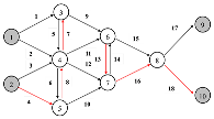
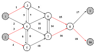
Taking the iconic fishbone network as our reference—originally unveiled by Hu et al. [16]—we encounter a structure composed of 18 directed links intertwined with 4 pivotal centroid nodes. Among these, nodes 1 and 2 stand as the origins of trips, whereas nodes 9 and 10 serve as their destined endpoints, as vividly illustrated in Figure 1. The remaining nodes—3, 4, 5, 6, 7, and 8—function as non-centroid waypoints within this web.
Delving into the insights of Ng [39], one learns that ensuring complete observability of all links in any network demands the strategic deployment of at least m n sensors. Translated to the fishbone network, this mandates that no fewer than 67% of its links—specifically, 12 of them—must be equipped with sensors. Yet, an elegant nuance arises: the flow dynamics on the remaining six unmonitored links can be precisely deduced through the flow measurements captured on the instrumented links. Notably, the configuration of observed links granting full flow observability is not singular; in fact, there can be multiple distinct sensor arrangements, each associated with its own corresponding system of linear equations.
Table 2 presents the collection of new links for the network drawn in Figure 1. The second column of the table enumerates the links connected to each non-centroid node, while the last column denotes the sets of new links attached to each non-centroid node. It is clear that the new links allocated to each non-centroid node are unique and do not overlap with those assigned to other non-centroid nodes. Furthermore, the entire collection of these new link sets collectively constitutes the full set of links within the network.
In the approach for assigning new links, one link is chosen from each non-empty new link set to create a set of unobserved links. The flow on these unobserved links can be inferred from the flows of the remaining observed links. Notably, the structural characteristics of these new link sets guarantee that the matrix representing the unobserved links, denoted by T u , is invertible.
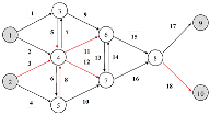
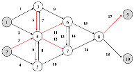
As illustrated in Table 3, layouts A and B showcase the linear equations alongside their corresponding accumulated inference errors for the flows on unobserved links, while red edges indicate links left without sensors (unobserved set U); black edges are instrumented links (observed set O), vividly demonstrating how these hidden flows can be deduced from the flow data collected on observed links. It is critical to recognize that the measurement errors originating from sensors installed on the observed links inevitably affect the accuracy of inferring unobserved link flows; these errors propagate through the inference system, culminating in compounded inference errors for the unobserved flows.
The total accumulated inference error affecting unobserved link flows is computed by incorporating the measurement errors from sensors on the observed links. Under the assumption that each sensor’s measurement error is uniform (for instance, 1 unit), Table 3 reveals that varying sensor placement strategies yield distinct levels of accumulated inference error within the same network. The inference error associated with an unobserved link flow correlates directly with the number of observed links involved in its inference: fewer observed links required translates to smaller inference errors. Consequently, to ensure full link flow observability while minimizing inference inaccuracies, the strategic goal must be to reduce either the maximum or the total count of observed links utilized in the inference of unobserved link flows.
The proposed BBA has been compared with two metaheuristic algorithms, PSO and GA, with independent measurement variance of the observed link flows (measurement error of 1 unit). Table 4 provides a comparison between the three models of the algorithms and illustrates their unobserved links and corresponding node sequencing across the final solution. The new links for the sensor location schemes of their results are shown in Table 5.
It can be observed that all three algorithms show a significant reduction in error after the initial iterations. However, the rate of convergence varies between the algorithms. The BBA Algorithm (red) exhibits a rapid decline in error early in the iterations compared to the other two algorithms. GA demonstrates the most consistent and slowest convergence, but eventually it reaches a lower error value of 22. The figure highlights the efficiency of the proposed algorithm in minimizing the error, as it converges faster and reaches the optimum compared to GA and PSO. This suggests that Algorithm 2 may be more effective in solving optimization problems with higher dimensions under the given conditions.

6.2. Sioux Falls Network

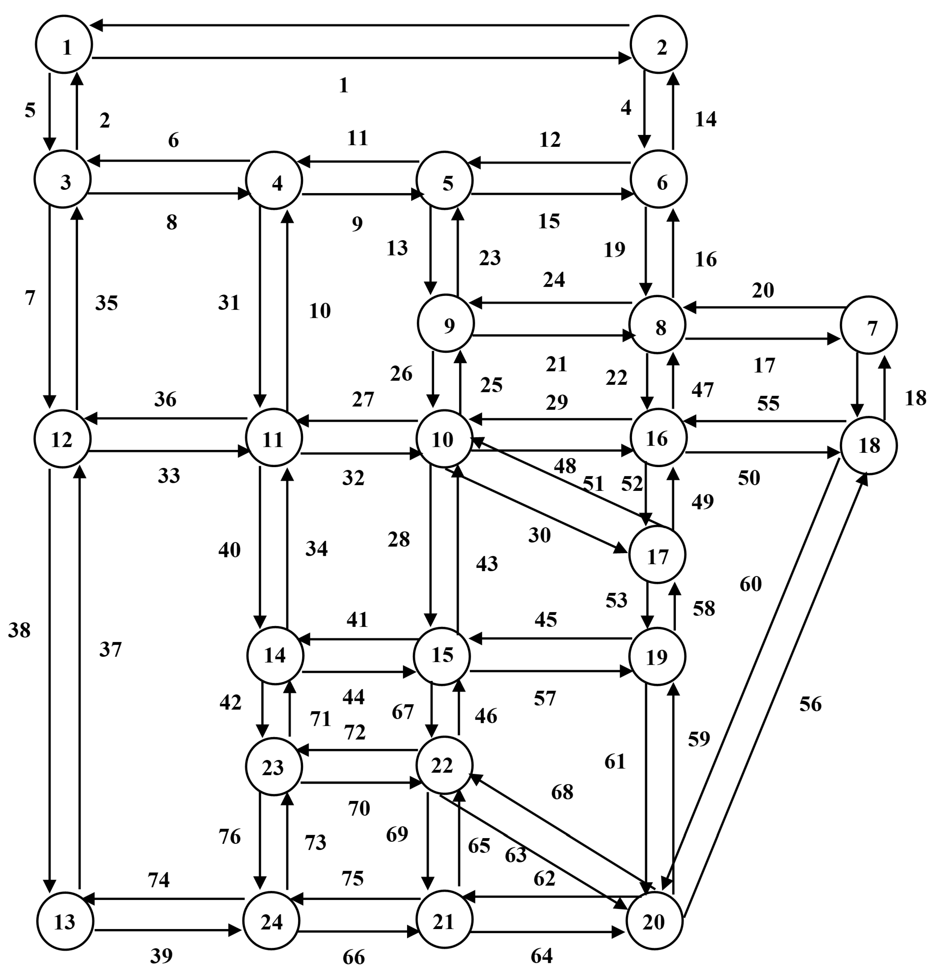
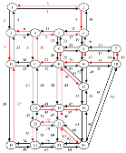
In this subsection, we analyze the accumulated inference error associated with inferring unobserved link flows in the Sioux Falls network, which consists of 24 non-centroid nodes and 76 links, as shown in Figure 2. The centroid nodes are not considered in this analysis, as per in Ng [10], who suggested that centroid nodes can be disregarded when collecting traffic count data for an entire day, since the origin and destination nodes can be treated as interchangeable for daily traffic counts.
Table 6 provides the sets of new links for the Sioux Falls network. Among the 24 non-centroid nodes, 23 nodes have non-empty sets of new links. According to the definition of new links, one link must be selected from each non-empty set of new links to be considered unobserved. This implies that 23 out of the 76 total links are selected to remain without sensors, while the remaining links are equipped with sensors. The resulting matrix, formed by removing one row from the node–link incidence matrix, retains full rank. The rank of the matrix equals the number of nodes minus one, which also represents the maximum number of unobserved links that can be inferred based on observed links.
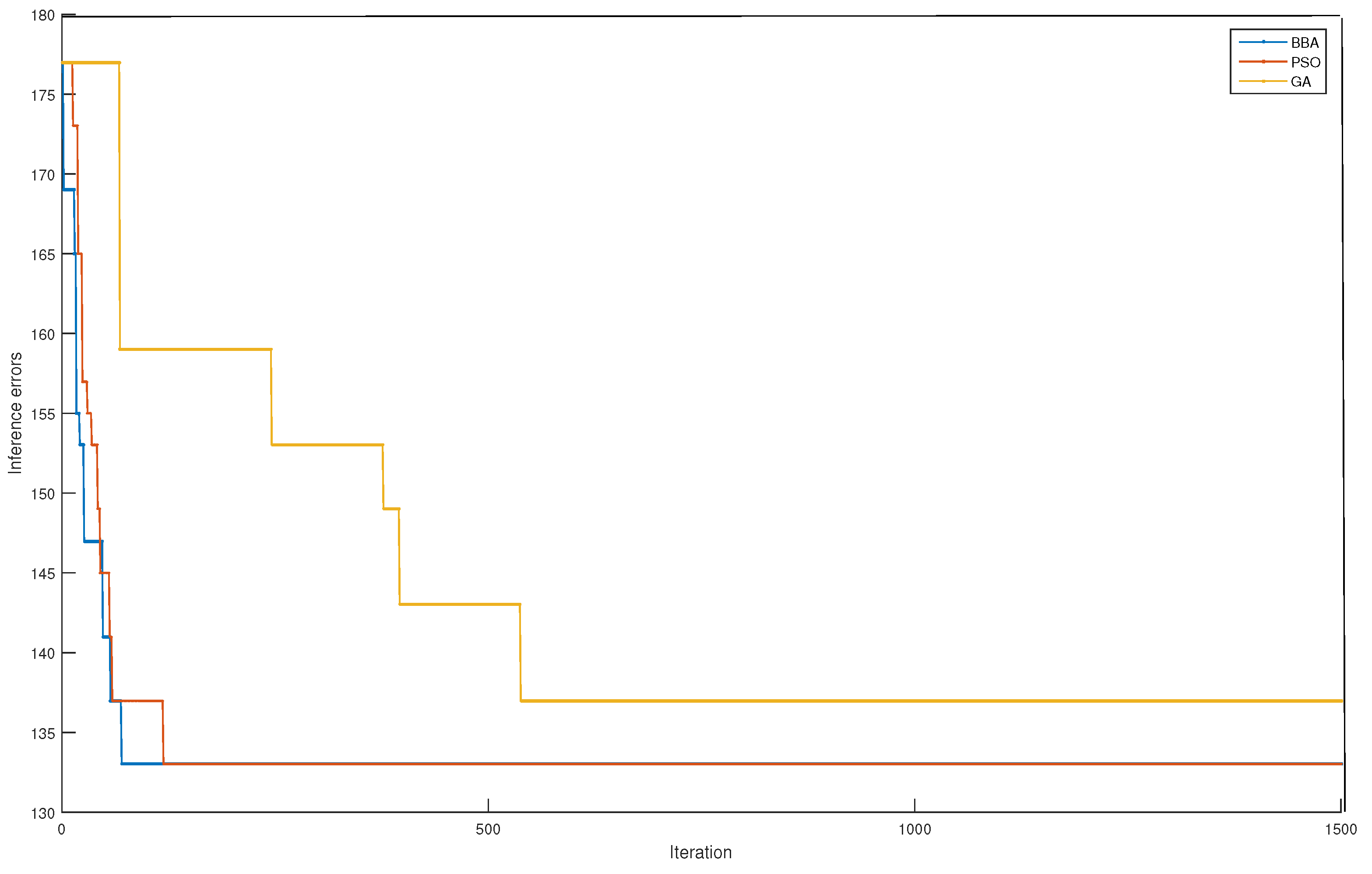
Assuming that all observed links are independent and subject to a measurement error of 1 unit, Figure 3 illustrates a comparison of accumulated inference errors, calculated using the proposed BBA Algorithm, PSO, and GA over 1500 iterations with 200 initial populations. The results show BBA and PSO quickly reaching the minimum accumulated inference error required to achieve full link flow observability in the Sioux Falls network of 133 after approximately 135 iterations, while GA shows a much slower reduction in error. It starts at a higher error value and gradually decreases, but its improvement plateaus at a higher error value compared to BBA and PSO. Overall, BBA performs the best in terms of error reduction, converging quickly to a low error value. PSO follows with a slower yet steady decrease in error, while GA shows the least improvement and converges at a higher error level. Figure 4 shows that, although all three algorithms exhibited similar distributions of unobserved links per node, with BBA and PSO each achieving 12 nodes (50%) with only one unobserved link and GA achieving 11 nodes (45.8%), the total inference error clearly distinguishes their effectiveness. GA recorded the highest error at 137, while both PSO and BBA achieved a lower and equal error of 133, indicating significantly better inference accuracy. Importantly, BBA converged faster than PSO, benefiting from its adaptive frequency tuning, directional echolocation strategy, and exploitation mechanisms that allow it to balance exploration and exploitation more efficiently. This rapid convergence combined with its consistent sensor placement and low inference error. The comprehensive comparison of the three algorithms, GA, PSO, and the proposed BBA, demonstrates the superior performance of BBA in terms of accuracy, consistency, and convergence speed. This highlights the robustness and practical efficiency of the proposed BBA Algorithm in solving the network transport problem.
Table 7 presents the optimal sensor placement schemes derived from BBA, PSO, and GA, together with the corresponding accumulated inference errors for the unobserved flows. In each case, the algorithms identify 23 unobserved links, which are visually marked in the network layouts by the red lines. The right-hand column of the table lists the cumulative error values (e.g., Error 137, Error 133), which quantify the degree of uncertainty propagated through the inference process when reconstructing the flows on unobserved links. Larger error values imply stronger propagation of measurement inaccuracies, highlighting the sensitivity of the system to sensor placement. The results illustrate that although all three methods produce the same number of unobserved links (23), they differ in how the inference equations distribute and accumulate errors across the network. For example, a total error of 133 indicates that while the inferred flows are uniquely recoverable, the accuracy of certain links is more vulnerable to error amplification. This demonstrates that the transformation matrix T u is not unique: different sensor placement schemes can generate valid but distinct sets of inference equations, leading to variations in how errors are distributed, even when the number of unobserved links remains constant. Hence, the table highlights both the robustness of the inference model and the practical implications of sensor placement decisions on error propagation.

6.3. Barcelona Network

In this subsection, we analyze the accumulated inference error associated with inferring unobserved link flows in the Barcelona network. Figure 5 shows the base map was obtained from Google Maps (2025) and used as a background to visualize the studied transportation network and sensor placement, which consists of 1020 non-centroid nodes and 2522 links. As noted in the previous network, centroid nodes are excluded from this analysis.
The sets of new links for the Barcelona network. Among the 1020 non-centroid nodes, 828 nodes have non-empty sets of new links. According to the definition of new links, one link must be selected from each non-empty set of new links to be considered unobserved. This implies that 828 out of the 1020 total links are selected to remain without sensors, while the remaining links are equipped with sensors. The resulting matrix, formed by removing 192 rows from the node-link incidence matrix, retains full rank. The rank of the matrix equals the number of nodes minus 192, which also represents the maximum number of unobserved links that can be inferred based on observed links.
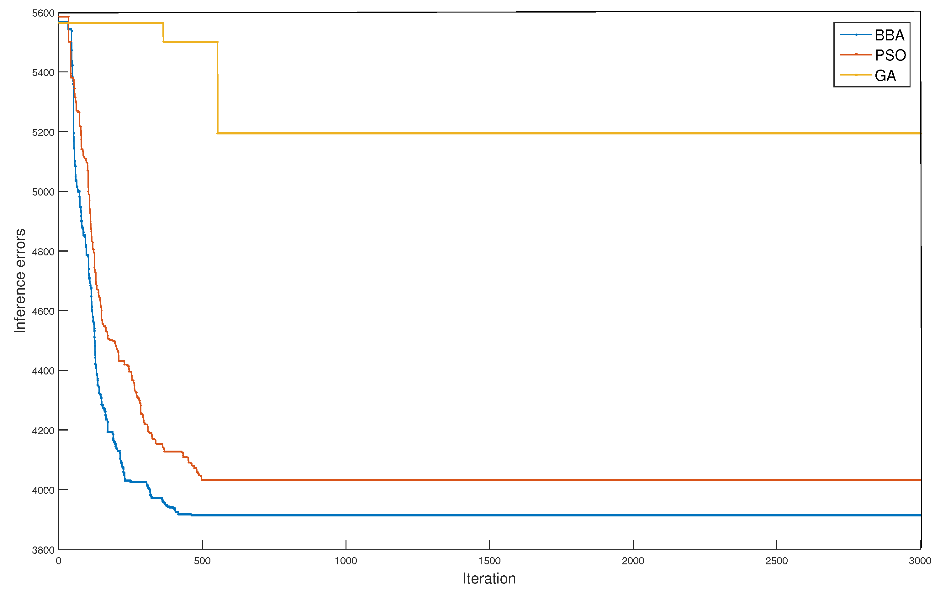
Figure 6 demonstrates inference errors in the Barcelona network for BBA, PSO, and GA with 300 initial populations algorithms over 3000 iterations, while further iterations beyond this point did not yield improved results. The comparison clearly shows that the BBA algorithm outperforms both PSO and GA in minimizing inference errors, achieving the lowest error of 3915 with faster and more stable convergence. PSO performs moderately well, reaching a slightly higher final error equal to 4032, while GA demonstrates poor performance, converging slowly and plateauing at a significantly higher error 5194 and requiring too many iterations to reach new solutions. In general, BBA appears to be the most efficient and effective optimization method among the three in this scenario.
Table 8 shows that BBA maintains low counts at higher link values and outperforms PSO in avoiding the long tail of poorly inferred nodes (e.g., PSO reaches up to 10 unobserved links). This supports BBA’s superiority not only in convergence but also in producing more uniformly inferred link distributions across the network.
From an algorithmic standpoint, the BBA exhibits several characteristics that make it particularly well suited for solving the TSLP under conditions of uncertainty. Inspired by the echolocation behavior of microbats, BBA efficiently balances global exploration and local exploitation through dynamic frequency tuning and adaptive pulse emission mechanisms. In binary search spaces, BBA employs a probabilistic transfer function to update candidate solutions based on their velocities, enabling effective traversal of the discrete sensor placement space. Notably, BBA dynamically adjusts its search behavior by modulating loudness and pulse rates in response to fitness improvements, which enhances its ability to escape local optima and converge to high-quality solutions. The mathematical formulation developed in this study supports error scenarios without requiring structural modifications to the optimization model.
These algorithmic properties are crucial in addressing the challenges posed by the TSLP, which features a high-dimensional, non-convex, and combinatorial solution space constrained by the need to maintain matrix invertibility (ensuring full flow observability). Traditional gradient-based or deterministic methods are inapplicable due to the non-differentiability and discrete nature of the objective functions. While only GA has been previously explored, BBA demonstrated superior performance in both convergence speed and solution quality, as validated in the experiments on the fishbone, Sioux Falls, and Barcelona networks. Its adaptive and memory-informed search strategy allows BBA to outperform competing methods, particularly in large-scale and complex network scenarios. These findings support the choice of BBA as the optimization engine in the proposed framework and underscore its potential in real-world traffic monitoring applications.
While the proposed framework successfully addresses the TSLP under measurement uncertainty, some limitations remain. First, our current experiments assumed uniform sensor errors for simplicity. However, incorporating non-uniform or heterogeneous measurement errors is a straightforward extension of the model, as the mathematical formulation already supports link-dependent error structures. This will be addressed in future work to more closely reflect real-world sensing conditions. Second, we did not explore multi-objective approaches for sensor placement. Practical traffic monitoring often involves multiple goals beyond flow inference accuracy, such as improving origin–destination (O/D) estimation, supporting screen-line analysis, or enabling reliable path reconstruction. Extending the model to explicitly handle such multi-objective trade-offs would further enhance its applicability for transportation planning and operations. Finally, although the current formulation demonstrates robustness and scalability, future studies could investigate hybrid optimization strategies and adaptive parameter control to strengthen performance consistency across diverse network scenarios.

7. Conclusions

This study addressed the TSLP for achieving full link flow observability under the realistic constraint of sensor measurement uncertainty. Recognizing the limitations of existing methods—particularly their reliance on idealized, error-free sensor assumptions and their scalability challenges in large networks—we proposed a novel, scalable optimization framework that integrates error propagation modeling into the sensor placement decision process. Two nonlinear integer optimization models were developed to minimize both the maximum and total accumulated inference errors in unobserved link flows. These models explicitly capture the impact of measurement uncertainty and leverage a node-based flow inference structure, which avoids the computational burden of path enumeration while ensuring the uniqueness and solvability of the network observability problem. The use of LU decomposition enabled efficient and numerically stable inversion of the matrix systems arising from unobserved link selection. To solve these complex, non-convex optimization problems, the BBA is adopted as a metaheuristic engine—not to compare metaheuristics per se but to provide an effective mechanism for exploring the vast and discrete search space of sensor configurations. BBA’s dynamic balance between global exploration and local exploitation, combined with its adaptive frequency tuning, proved particularly effective in navigating the high-dimensional nature of large transportation networks. The proposed framework was tested on three networks of varying complexity: the synthetic fishbone network, the benchmark Sioux Falls network, and a real-world Barcelona city network. The results demonstrated that the proposed method not only achieves full observability with the minimum number of sensors but also significantly reduces the propagation of inference errors. The approach consistently outperformed traditional techniques such as GA and PSO, especially in terms of convergence speed and solution quality in large-scale networks. In conclusion, this study presents a robust, scalable, and uncertainty-aware methodology for sensor placement in transportation networks. It bridges the gap between theoretical observability models and practical traffic monitoring applications by explicitly addressing measurement errors and computational feasibility. The integration of the BBA Algorithm as a scalable optimizer further enhances the framework’s applicability to real-world, large-scale urban systems. Future work may extend this framework to incorporate dynamic traffic conditions, heterogeneous sensor types, and multi-objective formulations that balance cost, resilience, and data accuracy.

Author Contributions

Conceptualization, M.O. and A.A.A.; Formal analysis, A.A.A.; Methodology, M.O.; Software, A.A.A.; Writing—original draft, A.A.A.; Writing—review and editing, M.O. All authors have read and agreed to the published version of the manuscript.

Funding

This research received no external funding.

Institutional Review Board Statement

Not applicable.

Informed Consent Statement

Not applicable.

Data Availability Statement

The data presented in this study are available on request from the corresponding author. The data are not publicly available due to privacy.

Conflicts of Interest

The authors declare no conflicts of interest.

References

  1. Owais, M. Deep learning for integrated origin–destination estimation and traffic sensor location problems. IEEE Trans. Intell. Transp. Syst. 2024, 25, 6501–6513. [Google Scholar] [CrossRef]
  2. Mehr, N.; Horowitz, R. A submodular approach for optimal sensor placement in traffic networks. In Proceedings of the 2018 Annual American Control Conference (ACC), Milwaukee, WI, USA, 27–29 June 2018; IEEE: New York, NY, USA, 2018; pp. 6353–6358. [Google Scholar]
  3. Li, R.; Mehr, N.; Horowitz, R. Submodularity of optimal sensor placement for traffic networks. Transp. Res. Part B Methodol. 2023, 171, 29–43. [Google Scholar] [CrossRef]
  4. Bianco, L.; Confessore, G.; Gentili, M. Combinatorial aspects of the sensor location problem. Ann. Oper. Res. 2006, 144, 201–234. [Google Scholar] [CrossRef]
  5. Castillo, E.; Grande, Z.; Calviño, A.; Szeto, W.Y.; Lo, H.K. A state-of-the-art review of the sensor location, flow observability, estimation, and prediction problems in traffic networks. J. Sens. 2015, 2015, 903563. [Google Scholar] [CrossRef]
  6. Gentili, M.; Mirchandani, P.B. Locating sensors on traffic networks: Models, challenges and research opportunities. Transp. Res. Part C Emerg. Technol. 2012, 24, 227–255. [Google Scholar] [CrossRef]
  7. Owais, M. Traffic sensor location problem: Three decades of research. Expert Syst. Appl. 2022, 208, 118134. [Google Scholar] [CrossRef]
  8. Owais, M.; Moussa, G.S.; Hussain, K.F. Sensor location model for O/D estimation: Multi-criteria meta-heuristics approach. Oper. Res. Perspect. 2019, 6, 100100. [Google Scholar] [CrossRef]
  9. Yang, H.; Zhou, J. Optimal traffic counting locations for origin–destination matrix estimation. Transp. Res. Part B Methodol. 1998, 32, 109–126. [Google Scholar] [CrossRef]
  10. Ng, M. Partial link flow observability in the presence of initial sensors: Solution without path enumeration. Transp. Res. Part E Logist. Transp. Rev. 2013, 51, 62–66. [Google Scholar] [CrossRef]
  11. Owais, M.; Moussa, G.S.; Hussain, K.F. Robust deep learning architecture for traffic flow estimation from a subset of link sensors. J. Transp. Eng. Part A Syst. 2020, 146, 04019055. [Google Scholar] [CrossRef]
  12. Danczyk, A.; Liu, H.X. A mixed-integer linear program for optimizing sensor locations along freeway corridors. Transp. Res. Part B Methodol. 2011, 45, 208–217. [Google Scholar] [CrossRef]
  13. Owais, M.; Shahin, A.I. Exact and heuristics algorithms for screen line problem in large size networks: Shortest path-based column generation approach. IEEE Trans. Intell. Transp. Syst. 2022, 23, 24829–24840. [Google Scholar] [CrossRef]
  14. Yang, H.; Gan, L.; Tang, W. Determing cordons and screen lines for origin-destination trip studies. In Proceedings of the Eastern Asia Society for Transportation Studies, Hanoi, Vietnam, 24–27 October 2001; Volume 3. [Google Scholar]
  15. Gentili, M.; Mirchandani, P.B. Locating active sensors on traffic networks. Ann. Oper. Res. 2005, 136, 229–257. [Google Scholar] [CrossRef]
  16. Hu, S.R.; Peeta, S.; Chu, C.H. Identification of vehicle sensor locations for link-based network traffic applications. Transp. Res. Part B Methodol. 2009, 43, 873–894. [Google Scholar] [CrossRef]
  17. Salari, M.; Kattan, L.; Lam, W.H.; Lo, H.; Esfeh, M.A. Optimization of traffic sensor location for complete link flow observability in traffic network considering sensor failure. Transp. Res. Part B Methodol. 2019, 121, 216–251. [Google Scholar] [CrossRef]
  18. Shao, M.; Sun, L.; Shao, X. Sensor location problem for network traffic flow derivation based on turning ratios at intersection. Math. Probl. Eng. 2016, 2016, 9012724. [Google Scholar] [CrossRef]
  19. Xie, C.; Shao, M.; Sun, L. Superiority proof of “incoming layout” for full link flow observability under uncertainty. Transp. Res. Part B Methodol. 2024, 190, 103090. [Google Scholar] [CrossRef]
  20. Xu, X.; Lo, H.K.; Chen, A.; Castillo, E. Robust network sensor location for complete link flow observability under uncertainty. Transp. Res. Part B Methodol. 2016, 88, 1–20. [Google Scholar] [CrossRef]
  21. Owais, M.; Matouk, A.E. A factorization scheme for observability analysis in transportation networks. Expert Syst. Appl. 2021, 174, 114727. [Google Scholar] [CrossRef]
  22. Contreras, S.; Kachroo, P.; Agarwal, S. Observability and sensor placement problem on highway segments: A traffic dynamics-based approach. IEEE Trans. Intell. Transp. Syst. 2015, 17, 848–858. [Google Scholar] [CrossRef]
  23. Yu, X.; Ma, S.; Zhu, N.; Lam, W.H.; Fu, H. Ensuring the robustness of link flow observation systems in sensor failure events. Transp. Res. Part B Methodol. 2023, 178, 102849. [Google Scholar] [CrossRef]
  24. Hu, X.; Fan, Y. Sensor placement considering the observability of traffic dynamics: On the algebraic and graphical perspectives. Transp. Res. Part B Methodol. 2024, 189, 103057. [Google Scholar] [CrossRef]
  25. Castro-Triguero, R.; Murugan, S.; Gallego, R.; Friswell, M.I. Robustness of optimal sensor placement under parametric uncertainty. Mech. Syst. Signal Process. 2013, 41, 268–287. [Google Scholar] [CrossRef]
  26. Houssein, E.H.; Saad, M.R.; Djenouri, Y.; Hu, G.; Ali, A.A.; Shaban, H. Metaheuristic algorithms and their applications in wireless sensor networks: Review, open issues, and challenges. Clust. Comput. 2024, 27, 13643–13673. [Google Scholar] [CrossRef]
  27. Almutairi, A.; Owais, M. Active traffic sensor location problem for the uniqueness of path flow identification in large-scale networks. IEEE Access 2024, 12, 180385–180403. [Google Scholar] [CrossRef]
  28. Almutairi, A.; Yi, P.; Owais, M. New approach for estimating intersection control delay from passive traffic sensors at network level. IEEE Access 2024, 12, 2882–2900. [Google Scholar] [CrossRef]
  29. Fakhouri, A.A.; Soltani, R. Multi-objective robust optimization for the traffic sensors location problem. IEEE Access 2020, 9, 6225–6238. [Google Scholar] [CrossRef]
  30. Mitsakis, E.; Chrysohoou, E.; Salanova Grau, J.M.; Iordanopoulos, P.; Aifadopoulou, G. The sensor location problem: Methodological approach and application. Transport 2017, 32, 113–119. [Google Scholar] [CrossRef]
  31. Owais, M.; El Deeb, M.; Abbas, Y.A. Distributing portable excess speed detectors in AL Riyadh city. Int. J. Civ. Eng. 2020, 18, 1301–1314. [Google Scholar] [CrossRef]
  32. Shao, M.; Xie, C.; Sun, L. Optimization of network sensor location for full link flow observability considering sensor measurement error. Transp. Res. Part C Emerg. Technol. 2021, 133, 103460. [Google Scholar] [CrossRef]
  33. Gentili, M.; Mirchandani, P.B. Review of optimal sensor location models for travel time estimation. Transp. Res. Part C Emerg. Technol. 2018, 90, 74–96. [Google Scholar] [CrossRef]
  34. Castillo, E.; Nogal, M.; Rivas, A.; Sánchez-Cambronero, S. Observability of traffic networks. Optimal location of counting and scanning devices. Transp. B Transp. Dyn. 2013, 1, 68–102. [Google Scholar] [CrossRef]
  35. Castillo, E.; Gallego, I.; Sanchez-Cambronero, S.; Rivas, A. Matrix tools for general observability analysis in traffic networks. IEEE Trans. Intell. Transp. Syst. 2010, 11, 799–813. [Google Scholar] [CrossRef]
  36. Castillo, E.; Conejo, A.J.; Pruneda, R.E.; Solares, C. Observability in linear systems of equations and inequalities: Applications. Comput. Oper. Res. 2007, 34, 1708–1720. [Google Scholar] [CrossRef]
  37. Castillo, E.; Jimenez, P.; Menendez, J.M.; Conejo, A.J. The observability problem in traffic models: Algebraic and topological methods. IEEE Trans. Intell. Transp. Syst. 2008, 9, 275–287. [Google Scholar] [CrossRef]
  38. Castillo, E.; Rivas, A.; Jiménez, P.; Menéndez, J.M. Observability in traffic networks. Plate scanning added by counting information. Transportation 2012, 39, 1301–1333. [Google Scholar] [CrossRef]
  39. Ng, M. Synergistic sensor location for link flow inference without path enumeration: A node-based approach. Transp. Res. Part B Methodol. 2012, 46, 781–788. [Google Scholar] [CrossRef]
  40. He, S.X. A graphical approach to identify sensor locations for link flow inference. Transp. Res. Part B Methodol. 2013, 51, 65–76. [Google Scholar] [CrossRef]
  41. Bianco, L.; Cerrone, C.; Cerulli, R.; Gentili, M. Locating sensors to observe network arc flows: Exact and heuristic approaches. Comput. Oper. Res. 2014, 46, 12–22. [Google Scholar] [CrossRef]
  42. Zhou, X.; List, G.F. An information-theoretic sensor location model for traffic origin-destination demand estimation applications. Transp. Sci. 2010, 44, 254–273. [Google Scholar] [CrossRef]
  43. Fei, X.; Mahmassani, H.S. Structural analysis of near-optimal sensor locations for a stochastic large-scale network. Transp. Res. Part C Emerg. Technol. 2011, 19, 440–453. [Google Scholar] [CrossRef]
  44. Xing, T.; Zhou, X.; Taylor, J. Designing heterogeneous sensor networks for estimating and predicting path travel time dynamics: An information-theoretic modeling approach. Transp. Res. Part B Methodol. 2013, 57, 66–90. [Google Scholar] [CrossRef]
  45. Zhu, N.; Fu, C.; Ma, S. Data-driven distributionally robust optimization approach for reliable travel-time-information-gain-oriented traffic sensor location model. Transp. Res. Part B Methodol. 2018, 113, 91–120. [Google Scholar] [CrossRef]
  46. Fu, H.; Lam, W.H.; Shao, H.; Kattan, L.; Salari, M. Optimization of multi-type traffic sensor locations for estimation of multi-period origin-destination demands with covariance effects. Transp. Res. Part E Logist. Transp. Rev. 2022, 157, 102555. [Google Scholar] [CrossRef]
  47. Danczyk, A.; Di, X.; Liu, H.X. A probabilistic optimization model for allocating freeway sensors. Transp. Res. Part C Emerg. Technol. 2016, 67, 378–398. [Google Scholar] [CrossRef]
  48. Zhu, N.; Ma, S.; Zheng, L. Travel time estimation oriented freeway sensor placement problem considering sensor failure. J. Intell. Transp. Syst. 2017, 21, 26–40. [Google Scholar] [CrossRef]
  49. Yang, X.S.; Hossein Gandomi, A. Bat algorithm: A novel approach for global engineering optimization. Eng. Comput. 2012, 29, 464–483. [Google Scholar] [CrossRef]
  50. Gandomi, A.H.; Yang, X.S.; Alavi, A.H.; Talatahari, S. Bat algorithm for constrained optimization tasks. Neural Comput. Appl. 2013, 22, 1239–1255. [Google Scholar] [CrossRef]
  51. Umar, S.U.; Rashid, T.A.; Ahmed, A.M.; Hassan, B.A.; Baker, M.R. Modified Bat Algorithm: A newly proposed approach for solving complex and real-world problems. Soft Comput. 2024, 28, 7983–7998. [Google Scholar] [CrossRef]
  52. Arbelaez, A.; Mehta, D.; O’Sullivan, B.; Quesada, L. A constraint-based parallel local search for the edge-disjoint rooted distance-constrained minimum spanning tree problem. J. Heuristics 2018, 24, 359–394. [Google Scholar] [CrossRef]
  53. Mirjalili, S.; Mirjalili, S.M.; Yang, X.S. Binary bat algorithm. Neural Comput. Appl. 2014, 25, 663–681. [Google Scholar] [CrossRef]
  54. Yang, X.S. A new metaheuristic bat-inspired algorithm. In Nature Inspired Cooperative Strategies for Optimization (NICSO 2010); Springer: Berlin/Heidelberg, Germany, 2010; pp. 65–74. [Google Scholar]
  55. Golberg, D.E. Genetic algorithms in search, optimization, and machine learning. Addion Wesley 1989, 1989, 36. [Google Scholar]
  56. Kennedy, J.; Eberhart, R. Particle swarm optimization. In Proceedings of the Proceedings of ICNN’95-International Conference on Neural Networks, Perth, WA, Australia, 27 November–1 December 1995; IEEE: New York, NY, USA, 1995; Volume 4, pp. 1942–1948. [Google Scholar]
  57. Fierro, R.D. Numerical Linear Algebra; University of Chicago Department of Statistics: Chicago, IL, USA, 1998. [Google Scholar]
  58. Golub, G.H.; Van Loan, C.F. Matrix Computations, 4th ed.; Johns Hopkins University Press: Baltimore, MD, USA, 2013. [Google Scholar]
  59. Higham, N.J. Accuracy and Stability of Numerical Algorithms; SIAM: Philadelphia, PA, USA, 2002. [Google Scholar]
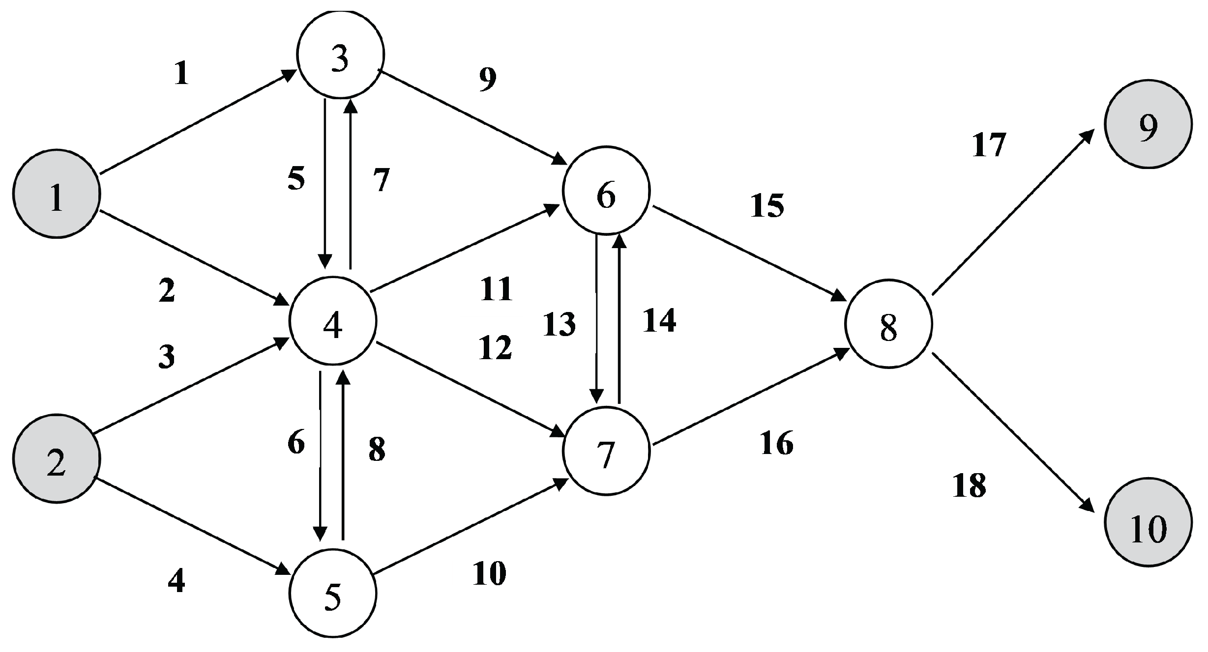
Figure 1. Fishbone network.
Applsci 15 10257 g001
Figure 2. Sioux Falls network.
Applsci 15 10257 g002
Figure 3. Inference errors in the Sioux Fall network using different metaheuristic algorithms.
Applsci 15 10257 g003
Figure 4. Frequency Distribution of Unobserved Links per Node for GA, PSO, and BBA.
Applsci 15 10257 g004
Figure 5. Barcelona network.
Applsci 15 10257 g005
Figure 6. Inference errors in the Barcelona network using different metaheuristic algorithms.
Applsci 15 10257 g006
Table 1. Initial parameters for BBA, PSO, and GA.
AlgorithmParametersValues
BBANumber of artificial batsdepends on the network’s dimension
f min 0
f max 2
A0.25
r0.5
ϵ 0.9
a0.9
γ 0.9
Stopping criterionMax iteration
PSONumber of particlesdepends on the network’s dimension
C 1 , C 2 2.2
WIs decreased linearly from 0.9 to 0.4
Max iterations500
Max velocity6
Stopping criterionMax iteration
GANumber of individualsdepends on the network’s dimension
SelectionRoulette wheel
Crossover (probability)One-point (0.9)
Mutation (probability)Uniform (0.005)
Max generationdepends on the network’s dimension
Stopping criterionMax generation
Table 2. New links of the fishbone network.
NodeConnected LinksNew Links
3{1, 5, 7, 9}{1, 5, 7, 9}
4{2, 3, 5, 6, 7, 8, 11, 12}{2, 3, 6, 8, 11, 12}
5{4, 6, 8, 10}{4, 10}
6{9, 11, 13, 14, 15}{13, 14, 15}
7{10, 12, 13, 14, 16}{16}
8{15, 16, 17, 18}{17, 18}
Table 3. Comparison of inference errors in two different layouts of Fishbone network.
Layout of SensorsLink Flow Inference EquationsError
AApplsci 15 10257 i001node 3: v 7 = v 5 + v 9 v 1
node 4:
v 8 = v 6 + v 7 + v 11 + v 12 v 2 v 3 v 5
node 5: v 4 = v 8 + v 10 v 6
node 6: v 15 = v 9 + v 11 + v 14 v 13
node 7: v 16 = v 10 + v 12 + v 13 v 14
node 8: v 18 = v 9 + v 10 + v 11 + v 12 v 17
31
BApplsci 15 10257 i002node 3: v 1 = v 5 + v 9 v 7
node 4:
v 3 = v 6 + v 7 + v 11 + v 12 v 2 v 5 v 8
node 5:
v 4 = v 7 + v 10 + v 11 + v 12 v 2 v 3 v 5
node 6: v 13 = v 9 + v 11 + v 14 v 15
node 7: v 16 = v 9 + v 10 + v 11 + v 12 v 15
node 8: v 18 = v 9 + v 10 + v 11 v 12 v 17
26
Table 4. Fishbone network models by GA, PSO, and BBA.
Layout of SensorsLink Flow Inference EquationsError
GAApplsci 15 10257 i003node 3: v 7 = v 5 + v 9 v 1
node 4: v 3 = v 1 + v 15 + v 16 v 2 v 4
node 5: v 6 = v 8 + v 10 v 4
node 6: v 11 = v 13 + v 15 v 9 v 14
node 7: v 12 = v 14 + v 16 v 10 v 13
node 8: v 18 = v 15 + v 16 v 17
22
PSOApplsci 15 10257 i004node 3: v 5 = v 1 + v 7 v 9
node 4: v 3 = v 15 + v 16 v 2 v 4
node 5: v 8 = v 4 + v 6 v 10
node 6: v 11 = v 13 + v 15 v 9 v 14
node 7: v 12 = v 14 + v 16 v 10 v 13
node 8: v 18 = v 15 + v 16 v 17
22
BBAApplsci 15 10257 i005node 3: v 5 = v 1 + v 9 v 7
node 4: v 3 = v 15 v 1 v 2 v 6 v 16
node 5: v 6 = v 8 + v 10 v 4
node 6: v 11 = v 13 + v 15 v 9 v 14
node 7: v 12 = v 14 + v 16 v 13 v 10
node 8: v 17 = v 15 + v 16 v 18
22
Table 5. New links and node sequencing between three models.
AlgorithmNodeConnected LinksNew LinksUnobserved Link
GA3{1, 5, 7, 9}{1, 5, 7, 9}7
5{4, 6, 8, 10}{4, 6, 8, 10}6
6{9, 11, 12, 13, 14, 15}{11, 13, 14, 15}11
7{10, 12, 13, 14, 16}{12, 16}12
4{2, 3, 5, 6, 7, 8, 11, 12}{2, 3}3
8{15, 16, 17, 18}{17, 18}18
PSO3{1, 5, 7, 9}{1, 5, 7, 9}5
5{4, 6, 8, 10}{4, 6, 8, 10}8
7{10, 12, 13, 14, 16}{12, 13, 14, 16}12
6{9, 11, 12, 13, 14, 15}{11,15}11
4{2, 3, 5, 6, 7, 8, 11, 12}{2, 3}3
8{15, 16, 17, 18}{17, 18}18
BBA3{1, 5, 7, 9}{1, 5, 7, 9}5
5{4, 6, 8, 10}{4, 6, 8, 10}6
6{9, 11, 12, 13, 14, 15}{11, 13, 14, 15}11
7{10, 12, 13, 14, 16}{12, 16}12
4{2, 3, 5, 6, 7, 8, 11, 12}{2, 3}3
8{15, 16, 17, 18}{17, 18}17
Table 6. Node-based new links of the Sioux Falls network.
NodeLinksSet of New Links
1{1, 2, 3, 5}{1, 2, 3, 5}
2{1, 3, 4, 14}{4, 14}
3{2, 5, 6, 7, 8, 35}{6, 7, 8, 35}
4{6, 8, 9, 10, 11, 31}{9, 10, 11, 31}
5{9, 11, 12, 13, 15, 23}{12, 13, 15, 23}
6{4, 12, 15, 16, 19}{16, 19}
7{17, 18, 20, 54}{17, 18, 20, 54}
8{16, 17, 19, 20, 21, 22, 24, 47}{21, 22, 24, 47}
9{13, 21, 23, 24, 25, 26}{25, 26}
10{25, 26, 27, 28, 29, 30, 32, 43, 48, 51}{27, 28, 29, 30, 32, 43, 48, 51}
11{10, 27, 31, 32, 33, 34, 36, 40}{33, 34, 36, 40}
12{7, 33, 35, 36, 37, 38}{37, 38}
13{37, 38, 39, 74}{39, 74}
14{34, 40, 41, 42, 44, 71}{41, 42, 44, 71}
15{28, 41, 43, 44, 45, 46, 57, 67}{45, 46, 57, 67}
16{22, 29, 47, 48, 49, 50, 52, 55}{49, 50, 52, 55}
17{30, 49, 51, 52, 53, 58}{53, 58}
18{18, 50, 54, 55, 56, 60}{56, 60}
19{45, 53, 57, 58, 59, 61}{59, 61}
20{56, 59, 60, 61, 62, 63, 64, 68}{62, 63, 64, 68}
21{62, 64, 65, 66, 69, 75}{65, 66, 69, 75}
22{46, 63, 65, 67, 68, 69, 70, 72}{70, 72}
23{42, 70, 71, 72, 73, 76}{73, 76}
24{39, 66, 73, 74, 75, 76}{}
Table 7. Sioux Fall network models by GA, PSO, and BBA.
Layout of SensorsLink Flow Inference EquationsError
GAApplsci 15 10257 i006node 1: v 3 = v 1 + v 5 v 2
node 2: v 4 = v 14 + v 2 v 5
node 3: v 6 = v 8 + v 2 + v 33 + v 39 v 5 v 36 v 74
node 4:
v 10 = v 31 + v 39 + v 33 + v 13 + v 19 v 36 v 74 v 16 v 23
node 5: v 9 = v 11 + v 13 + v 19 + v 5 v 23 v 16 v 2
node 6: v 15 = v 12 + v 19 + v 5 v 2 v 16
node 7: v 18 = v 20 + v 54 v 17
node 8: v 47 = v 22 + v 24 + v 16 + v 17 v 21 v 19 v 20
node 9: v 25 = v 26 + v 23 + v 21 v 13 v 24
node 10: v 43 = v 28 + v 39 + v 40 + v 53 + v 60 v 58 v 34
node 11:
v 27 = v 40 + v 19 + v 13 + v 39 + v 32 v 746 v 16 v 23 v 34
node 12: v 7 = v 35 + v 33 + v 39 v 36 v 74
node 13: v 37 = v 74 + v 38 v 39
node 14: v 44 = v 41 + v 40 + v 71 v 34 v 42
node 15:
v 46 = v 67 + v 39 + v 60 + v 42 + v 61 v 74 v 56 v 71 v 59
node 16:
v 29 = v 48 + v 52 + v 19 + v 21 + v 56 v 24 v 49 v 16 v 60
node 17: v 30 = v 51 + v 52 + v 53 v 58 v 49
node 18: v 55 = v 17 + v 50 + v 56 v 20 v 60
node 19: v 57 = v 45 + v 58 + v 61 v 53 v 59
node 20: v 63 = v 68 + v 59 + v 56 + v 62 v 61 v 60 v 64
node 21: v 65 = v 69 + v 66 + v 62 v 64 v 75
node 22: v 72 = v 71 + v 70 + v 66 + v 74 v 75 v 39 v 42
     node 23: v 76 = v 73 + v 66 + v 74 v 57 v 39
137
PSOApplsci 15 10257 i007node 1: v 5 = v 2 + v 3 v 1
node 2: v 1 = v 14 + v 1 v 3
node 3: v 8 = v 6 + v 3 + v 35 v 1 v 7
node 4: v 10 = v 31 + v 19 + v 13 + v 7 v 16 v 23 v 35
node 5: v 11 = v 9 + v 1 + v 16 + v 23 v 3 v 19 v 13
node 6: v 12 = v 15 + v 16 + v 1 v 3 v 19
node 7: v 17 = v 20 + v 54 v 18
node 8: v 47 = v 22 + v 54 + v 16 + v 24 v 18 v 19 v 21
node 9: v 25 = v 26 + v 23 + v 21 v 13 v 24
node 10:
v 43 = v 28 + v 40 + v 38 + v 60 + v 53 v 37 v 34 v 56 v 58
node 11:
v 27 = v 40 + v 38 + v 32 + v 19 + v 13 v 16 v 23 v 37 v 34
node 12: v 36 = v 33 + v 35 + v 38 v 7 v 37
node 13: v 74 = v 39 + v 37 v 38
node 14: v 44 = v 41 + v 40 + v 71 v 42 v 34
node 15:
v 46 = v 67 + v 38 + v 60 + v 42 + v 61 v 37 v 56 v 71 v 59
node 16:
v 29 = v 56 + v 48 + v 49 + v 19 + v 21 v 52 v 16 v 60 v 24
node 17: v 51 = v 30 + v 52 + v 58 v 49 v 53
node 18: v 50 = v 18 + v 55 + v 60 v 54 v 56
node 19: v 45 = v 57 + v 59 + v 53 v 58 v 61
node 20: v 63 = v 68 + v 59 + v 56 + v 62 v 61 v 60 v 64
node 21: v 66 = v 75 + v 76 + v 38 v 73 v 37
node 22: v 69 = v 65 + v 64 + v 73 + v 37 v 62 v 76 v 38
     node 23: v 70 = v 42 + v 72 + v 73 v 71 v 76
133
BBAApplsci 15 10257 i008node 1: v 1 = v 2 + v 3 v 5
node 2: v 14 = v 5 + v 4 v 2
node 3: v 6 = v 2 + v 7 + v 8 v 5 v 35
node 4: v 10 = v 7 + v 13 + v 19 + v 31 v 16 v 23 v 35
node 5: v 9 = v 5 + v 11 + v 13 + v 19 v 2 v 16 v 23
node 6: v 15 = v 5 + v 12 + v 19 v 2 v 16
node 7: v 18 = v 20 + v 54 v 17
node 8: v 47 = v 16 + v 22 + v 17 + v 24 v 19 v 21 v 20
node 9: v 25 = v 21 + v 23 + v 26 v 13 v 24
node 10:
v 43 = v 28 + v 40 + v 38 + v 53 + v 60 v 37 v 34 v 58 v 56
node 11:
v 27 = v 13 + v 19 + v 32 + v 40 + v 38 v 16 v 23 v 37 v 34
node 12: v 33 = v 7 + v 36 + v 37 v 35 v 38
node 13: v 39 = v 38 + v 74 v 37
node 14: v 41 = v 34 + v 44 + v 42 v 40 v 71
node 15:
v 46 = v 61 + v 42 + v 38 + v 60 + v 67 v 59 v 71 v 37 v 56
node 16:
v 29 = v 48 + v 49 + v 19 + v 21 + v 56 v 16 v 24 v 52 v 60
node 17: v 30 = v 51 + v 49 + v 53 v 52 v 58
node 18: v 50 = v 20 + v 55 + v 60 v 17 v 56
node 19: v 57 = v 58 + v 45 + v 61 v 53 v 59
node 20: v 63 = v 56 + v 62 + v 68 + v 59 v 60 v 61 v 64
node 21: v 66 = v 75 + v 38 + v 76 v 73 v 37
node 22: v 65 = v 62 + v 38 + v 76 + v 69 v 64 v 73 v 37
     node 23: v 70 = v 42 + v 72 + v 73 v 71 v 76
133
Table 8. Distribution of the Number of Unobserved Links per Node Across the GA, PSO, and BBA Algorithms.
Unobserved Links per NodeGAPSOBBA
1425436426
2304317331
3161140137
4272930
5253
6111
7000
8202
9010
10010
Disclaimer/Publisher’s Note: The statements, opinions and data contained in all publications are solely those of the individual author(s) and contributor(s) and not of MDPI and/or the editor(s). MDPI and/or the editor(s) disclaim responsibility for any injury to people or property resulting from any ideas, methods, instructions or products referred to in the content.