Abstract
Addressing the real-time control challenges within large-scale, complex resource-constrained project scheduling, this paper investigates control strategies to ensure the on-time initiation of critical task nodes during the execution of aviation cluster mission plans in the presence of disturbances. Conventional resource-constrained project scheduling problem (RCPSP) models typically treat task start times as the primary decision variables, overlooking the intrinsic link between task duration and resource allocation. Moreover, their reliance on intelligent optimization algorithms struggles to simultaneously balance solution accuracy and computational efficiency, thus failing to meet the demands of precise, real-time control. This paper proposes a real-time project schedule control system with the primary objective of preventing delays in critical tasks. The system aims to maximize the remaining anti-disturbance capacity under resource constraints, and establishes five control constraints tailored to the practical problem’s characteristics. The limitations of traditional approaches mainly lie in the fact that they take the start time of each task as the decision variable. When the scale of task quantity in the project is large, the decision dimension increases exponentially; meanwhile, the start times of various tasks are interdependent, leading to extremely complex constraint relationships. To overcome the limitations of traditional methods, this paper introduces a precise control method based on the Critical Path Transform Tree (CPTT). This method takes task duration as the decision variable, calculates the start time of each task using a recursive formula, and integrates expert heuristic knowledge to transform the dynamic network schedule from a “black box” to a “gray box” model. It effectively addresses the technical challenge of reverse mapping in the recursive formula, ultimately realizing precise and real-time control of the project schedule. The simulation results show that while maintaining high solution accuracy, the computational efficiency of the proposed control method is significantly improved to 1.6 s—compared with an average of 6.9 s for the adaptive differential evolution algorithm—thus verifying its effectiveness and practicality in real-time control applications.
1. Introduction
As a task force operation with multi-role and multi-phase attributes, aviation cluster missions require participating units of different functional roles (such as various types of unmanned aerial vehicles, UAVs) to collaborate closely according to predefined divisions of labor to achieve a unified mission objective. From the perspective of mission structure, the core tasks undertaken by each role can be further decomposed into subtasks covering multiple phases of the entire mission life cycle. The aviation cluster mission scenario focused on in this study is typically representative, taking the UAV cluster ground strike mission as an example: executing this mission requires coordinated cooperation among multiple types of UAVs, including reconnaissance UAVs, communication relay UAVs, attack UAVs, and aerial refueling tankers, forming a complete mission chain of “reconnaissance–communication–strike–assessment.” However, completing this mission is not merely about finishing the chain; there are often critical task nodes that must be executed on time. For instance, in this scenario, the strike task may have a fleeting time window, necessitating precise timing for execution.
The constraints that must be considered in this problem include the following:
- Mission constraints: Critical task nodes must be executed on time, which is the core objective of the mission.
- Sequential constraints: These manifest as sequential logical dependencies between the initiation and completion of subtasks. Due to airport runway capacity management, a subsequent UAV can only begin to taxi after the preceding one has taken off. The strike mission can only be executed after the reconnaissance UAV has completed its survey and the strike UAV has arrived at its designated strike position.
- Resource constraints: Each UAV has a limited amount of fuel to complete its respective subtasks. The duration of a UAV’s subtask is related to its flight speed; higher speeds result in greater fuel consumption.
- Flight performance constraints: The real-time flight speed of a UAV must comply with its flight performance capabilities, with an upper limit on flight speed.
- The task controllability constraint: Due to the specific circumstances of each task, it is not necessarily possible to compress the planned duration of all tasks. Additionally, whether a task is controllable depends on its current state.Tasks that are already completed are obviously uncontrollable. For tasks that are currently in progress, since their execution requires certain resources and once a task starts, it means those resources may have already been put into use, we no longer make ad hoc adjustments to tasks that are in progress. This approach also serves to reduce the cognitive load on the executor. Only tasks that have not yet started at the current time are controllable.
This creates a complex trade-off scenario: Within the overall mission, several tasks serve as critical task nodes and must be executed on time. The total task duration of a single UAV is composed of the flight transit time and execution time of its subtasks, while the start time of a task is affected by inter-task dependencies. When a preceding task incurs a delay, it is necessary to shorten the duration of certain subsequent tasks to ensure the on-time execution of critical task nodes. Increasing the flight speed can shorten the flight transit time but will increase fuel consumption; adjusting the refueling duration can alter the amount of fuel transferred. Except for refueling and flight transit, the execution time of other subtasks is fixed. Changes in the duration of a task will, in turn, affect the start times of other dependent tasks.
During the aviation cluster mission planning phase, it is essential to identify the critical mission nodes that must be executed on time. Typically, such missions undergo detailed pre-planning to ensure the feasibility of the initial scheduling scheme. It should be noted that only critical mission nodes require on-time execution; minor time deviations for other tasks are acceptable. Fuel is a “weak” constraint, tolerating “small” delays without compromising safety. Usually, during the mission planning phase, a threshold is set for the fuel level of each UAV upon completing its return. The planned scheme must ensure that all UAVs land with fuel levels above this threshold. During mission execution, the remaining fuel upon task completion and return is predicted in real time for each UAV. If the predicted value falls below the threshold, the current fuel is considered insufficient, and control measures are required. Therefore, while factors such as climate and air density may cause discrepancies between planned and actual fuel consumption, as long as the alert threshold is satisfied, no control action is needed.
However, deviations from the original plan are inevitable during the execution phase, making it impossible to adhere strictly to the planned timeline. Consequently, when disturbances occur, a plan that was initially deemed feasible may no longer guarantee the on-time initiation of critical nodes, potentially leading to the failure of the overall mission. Therefore, it is not sufficient to merely formulate an optimal plan beforehand. It is also crucial to implement real-time control during the execution phase—adjusting task start times and durations within the constraints of limited fuel—to ensure that mission objectives are successfully met even in the face of disturbances.
Existing research on task and mission scheduling is primarily applied in fields such as project management, production planning and management, traffic management, and operations planning and management. The principal techniques can be divided into two main branches: network planning techniques and the resource-constrained project scheduling problem (RCPSP).
Network planning originated in the late 1950s. Based on network diagrams, they visually represent the sequence and interdependencies of various activities in a planned task, and identify critical paths and critical activities through the calculation of time parameters—serving as a scientific planning and management method. The core technologies of network planning include the Program Evaluation and Review Technique (PERT) [1] and the Critical Path Method (CPM), which are essential for collaborative manufacturing and enterprise resource management in modern large-scale enterprises [2]. With the expansion of application fields, network planning techniques have continuously evolved into new forms to adapt to complex scenarios (e.g., uncertain interdependencies and uncertain activity durations). Currently, developed variants include the Graphic Evaluation and Review Technique (GERT) [3], Venture Evaluation and Review Technique (VERT), and Decision Critical Path Method (DCPM) [4]. However, a limitation of network planning techniques is that they do not consider resource constraints. In practical scenarios, however, resource constraints are universally prevalent; neglecting them leads to distorted calculations of critical paths and slack time. To address this issue, researchers have begun investigating resource-constrained project scheduling problems.
The resource-constrained project scheduling problem (RCPSP), first proposed by Davis [5], addresses how to optimally schedule the start time of each task under resource and task sequential constraints to achieve an optimal objective. The RCPSP model later evolved into many branches, including Job Shop scheduling and Flexible Open Shop Scheduling. A limitation of the classic model, however, is that it does not consider the specific matching between resources and tasks, nor can it explicitly determine if a resource meets the requirements to perform a task. Building on this classic model, Levchuk et al. proposed an improved model [6] that specifies task execution conditions based on task requirements and resource capabilities, more closely reflecting practical situations. To better simulate the complexity of real-world environments, researchers have proposed various extended RCPSP models: for scenarios where a task has multiple execution modes (each mode corresponding to different durations and resource requirements), the Multi-Mode Resource-Constrained Project Scheduling Problem (MRCPSP) [7] was developed; for labor-intensive projects, where the skills of human resources affect task durations (resulting in dynamic changes in actual task durations based on the skill level of allocated resources), the Skill-Constrained RCPSP (MS-RCPSP) [8] was introduced; and for uncertainties in real-world problems (e.g., task durations, resource availability, and even task lists), proactive RCPSP and reactive RCPSP were proposed [9]. Proactive scheduling incorporates robustness into baseline plan formulation: it models uncertain parameters using fuzzy random variables or triangular fuzzy numbers, and aims to maximize the confidence level that the plan meets specific objectives [10]. Reactive scheduling dynamically adjusts plans after disturbances occur, with its core being the design of efficient repair strategies [11].
Solution methods for RCPSP can be roughly divided into three categories: exact algorithms, intelligent optimization algorithms, and machine learning. Exact algorithms aim to find the optimal solution, primarily including branch and bound (B & B) [12], integer linear programming (ILP) [13], and constraint programming (CP). These methods are effective for small-scale instances; however, due to the NP-hard nature of the problem, exact algorithms see an exponential increase in the solution time when dealing with large-scale instances, failing to meet practical needs. Given the large scale of real-world problems such as production planning management, people have begun to sacrifice solution accuracy in exchange for faster solution speed to improve solving efficiency. Intelligent optimization algorithms improve solution efficiency by performing intelligent searches in the solution space to quickly approximate the global optimal solution. Representative methods include genetic algorithms, tabu search, and simulated annealing, which have been successfully applied to RCPSP [14]. The essence of intelligent optimization algorithms lies in abandoning the mathematically provable absolute optimal solution, thereby avoiding rigorous derivation for non-linear, non-differentiable, and high-dimensional mathematical problems. They are essentially random search methods that significantly narrow down the solution space requiring focused search, enabling them to provide a high-quality feasible solution for complex problems within an acceptable timeframe. However, such methods often converge only at local optima, leading to a substantial reduction in accuracy. With the development of artificial intelligence, combining machine learning techniques with traditional optimization methods has become a cutting-edge trend: reinforcement learning agents learn when and how to adjust schedules, demonstrating great potential in addressing scheduling problems in dynamic and uncertain environments [15]. Moreover, the offline learning–online decision-making framework of reinforcement learning can be implemented; although the training process is time-consuming, the decision-making speed during actual execution is relatively fast. However, reinforcement learning has poor generalization ability. For different scheduling problems or different network planning structures of the same scheduling problem, it is necessary to train different agents.
Compared with traditional project schedule management and production planning management, an aviation cluster mission has some new characteristics: firstly, extremely high control precision. In project schedule management, the management cycle is usually in days or weeks. Due to the high speed of aircraft, the time precision of aviation cluster mission plans is usually accurate to minutes. Secondly, extremely strict control objectives. Due to the complexity of the collaboration among various types of aircraft, tasks have strict time window constraints and extremely high planning requirements. For example, in the ground strike mission of a drone cluster, if the strike time is advanced or delayed, it may cause the supporting resources required for the strike to be unavailable, which may eventually lead to the failure of the entire mission due to a small disturbance affecting a large number of aircraft. Thirdly, extremely fast solving speed of control strategies. Precisely because of the first two characteristics, it is necessary to quickly eliminate disturbances.
In summary, RCPSP and its improved task scheduling models are all NP-hard combinatorial optimization problems. Currently, there is no algorithm that can simultaneously meet the accuracy and efficiency requirements of aviation cluster missions. As a result, current research primarily focuses on optimal scheduling for pre-event plan formulation, lacking the development of real-time closed-loop feedback scheduling control systems.
Schedule control refers to the monitoring and control of deviations in task progress and resource status during project execution. In large-scale production lines, various disturbances inevitably affect the production schedule, leading to delays or a decline in quality [16,17]. To manage production progress, Earned Value Management (EVM) is commonly used. This method involves establishing a series of earned value metrics, tracking these metrics at key checkpoints, and identifying and analyzing deviations from the planned progress to guide the formulation of corrective actions [18,19]. However, EVM’s primary focus is on identifying deviations; it does not directly, rapidly, or precisely generate a control plan to correct them. Therefore, EVM is often applied to long-term projects that are not highly time-sensitive and is less suitable for schedule control in contexts that demand high temporal sensitivity. Similarly, in the field of flight management, task progress control mainly involves managing the impact of one flight’s delay on subsequent flights. Existing research in this area focuses on developing flight delay propagation models and flight recovery models. These models are used to calculate the cascading effect of a preceding flight’s delay and subsequently generate a flight recovery plan [20,21,22,23]. In operational planning and management, existing military mission planning and control primarily focus on research related to replanning modeling [24,25,26]. Replanning mainly involves establishing a mapping model between task platform allocation schemes and mission accomplishment [27,28]. When unexpected events occur and it is assessed that the mission cannot be completed as scheduled, the task platform allocation scheme is rescheduled to ensure the smooth achievement of the operational mission. Research on collaborative planning control mainly focuses on defining process frameworks and fundamental principles/methods [29]. Most battle management systems emphasize the hierarchical architecture and key technologies of the system, but lack the establishment of specific planning control models and real-time control systems [30].
In summary, existing research fails to effectively address the real-time control problem for the execution of aviation cluster mission plans, presenting the following shortcomings: Firstly, a real-time schedule control system has not been established. In practical applications, it is necessary not only to monitor schedule deviations but also to compute a control solution within a very short timeframe. This necessitates the development of a dedicated control system. Secondly, in current schedule control problems, the on-time execution of critical task nodes is not taken as the control objective. Thirdly, there is a lack of a schedule control algorithm that can simultaneously satisfy the requirements for both solution accuracy and computational efficiency. Earned Value Management (EVM), a common method in project management, is primarily used to guide schedule adjustments and is unsuitable for highly time-sensitive, real-time control. Meanwhile, although various scheduling models like RCPSP and its variants exist, they present a trade-off: exact algorithms cannot meet the demands for computational speed, while heuristic algorithms cannot guarantee the required level of solution accuracy.
Existing research on schedule control lacks an exploration of strategies for precise, real-time control. The fundamental reason for this is the difficulty in solving the “reverse mapping” problem—that is, determining the required duration for each task based on a desired completion time for a critical task. This challenge arises because the structure of the network plan changes dynamically, causing the corresponding recursive time calculation formulas to change as well.
In summary, to address the shortcomings of existing research, our main contributions are as follows:
- 1.
- We established a real-time control system for aviation cluster mission plans operating under practical resource constraints, with the objective of ensuring the on-time execution of critical task nodes.
- 2.
- We propose a precise control method based on a Critical Path Transform Tree. This method solves the difficult reverse mapping problem for dynamically changing network plan recursion formulas. We have validated this approach through simulations, demonstrating its ability to achieve precise control.
2. Model
2.1. Problem Description
The refueling control problem for a collaborative mission network is a type of resource-constrained project scheduling problem (RCPSP) and can be considered an extension of the traditional Job Shop scheduling problem. The control problem itself can be viewed as a real-time dynamic scheduling challenge. The problem is described by the following characteristics and constraints:
- 1.
- On-time Execution of Critical Nodes: The primary and most critical objective of the control system is to ensure that critical task nodes are executed punctually.
- 2.
- Sequential Constraints: Precedence constraints exist among the various subtasks of different UAVs. This creates interdependencies where the start time of one subtask is dependent on the completion time of others.
- 3.
- Disturbance Management: The plan is subject to disturbances during execution, which can cause delays and jeopardize the on-time start of critical nodes. This necessitates a control mechanism for the schedule, but one that avoids frequent or excessive plan revisions (i.e., schedule instability).
- 4.
- Fuel Sufficiency: Each UAV must have enough fuel to complete all of its assigned tasks.
- 5.
- Time-Resource Trade-off: The duration of a UAV’s subtask is correlated with its flight speed; higher speeds reduce flight time but lead to greater fuel consumption.
- 6.
- Performance Limits: The real-time flight speed of each UAV must remain within its specified performance limits.
Mathematical Description: A group mission is jointly executed by UAVs, denoted as . The i-th UAV, , undertakes subtasks. In their order of execution, these subtasks are , and their respective durations are .
In the group’s network plan diagram, the horizontal axis represents time, and the vertical axis represents the different UAVs; therefore, the vertical axis has a row, as shown in Figure 1. Tasks are represented by directed solid lines with arrowheads. From a horizontal perspective, each row in the diagram contains multiple arrow lines, which correspond to the subtasks of UAV . The length of a line represents the duration of that task.
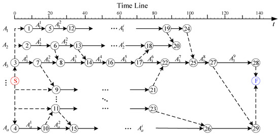
Figure 1.
Schematic of the network plan.
The start and end times of a task are nodes, depicted as numbered circles. The node at the arrowhead represents the completion of the task corresponding to that arrow line, while the node at the tail of the arrow represents the start of the task. The S node and F node represent the global start node and global end node, respectively, and are colored red and blue for clear identification. The temporal relationships between the subtasks of different UAVs are indicated by arrows.
The start time and end time of a task correspond to the positions and on the time axis for the task’s start node and end node , respectively.
Thus, the time interval between the start time and end time of task is the task duration, i.e.,
In the network plan diagram, a dashed line represents a dummy activity. Its task duration is zero, and it is used only to express coordination relationships between tasks.
For any given task , all activities pointing to its start node represent the predecessor tasks of . This means that task can only begin after all of its predecessor tasks are completed. Conversely, all activities flowing from its end node represent the successor tasks of , meaning its successor tasks can only begin after task itself is completed.
Let the set of predecessor tasks for task be , and let the set of successor tasks be . Then, the following constraints apply:
The primary resource constraint for completing the overall mission is the fuel capacity of each unmanned aerial vehicle (UAV). Let the total fuel (takeoff fuel) of UAV be . The higher its flight speed, the shorter the duration of the flight path mission, but the more fuel is consumed. The relationship between this UAV’s fuel consumption rate and its flight speed is as follows:
Thus, the relational expression for the real-time remaining fuel function of the UAV (assuming no in-air refueling) is as follows:
Let the set of flight path subtasks be denoted by . For a specific flight path subtask assigned to a UAV, its duration is dependent on the flight speed:
Let the UAV be the refueling aircraft (tanker), with a refueling rate of . The set of UAVs with in-flight refueling capability is denoted as . Then, for a UAV that can be refueled in-flight, where ∈, its subtasks must include an in-flight refueling task, . If refueling is not required for this mission, then let = 0. For UAV , the function for its real-time remaining fuel is expressed as follows:
2.2. Control System Modeling
In solving the resource-constrained project scheduling problem (RCPSP) and its extensions, the start time of each task is typically treated as the decision variable. The dependencies between tasks are converted into temporal constraints on these variables, while the task durations are considered to be constant.
This type of scheduling problem is NP-hard, making the complexity of exact solution algorithms prohibitively large. Consequently, heuristic algorithms have traditionally been employed. However, due to the presence of disturbances during the execution phase, task durations can change dynamically. This causes the computational complexity for dynamic rescheduling with this method to become extremely high.
Control algorithms are required to achieve high solution accuracy for critical task nodes while maintaining low time complexity. To address this issue, we establish a real-time control system. In this system, the duration of each task is the state variable , the time deviation at critical task nodes is the output variable , and the decision variable is the control input . To reduce the decision space, the start time of each task is calculated using the recursive formula of a network plan. As long as the duration and dependencies of each task are determined, the start times can be fixed. We have formulated this recursive formula as the system’s output equation.
- 1.
- State Variable
Let the task vector be denoted by , which represents the aggregate set of all subtasks to be performed by all UAVs. Here, is the identifier for a specific subtask.
The state variable is then defined as the vector of task durations corresponding to each subtask in the task vector m.
In this expression, denotes the duration of subtask at time instance . Under perfectly ideal planning conditions, the actual duration of each subtask would be equal to its scheduled time, that is
Therefore, the planned state variable is as follows: .
However, tasks are often subject to disturbances during the actual execution process. Let the disturbance time of task at time t be . Then, the state of task under this condition is as follows:
- 2.
- Output Variable
The output variable quantifies the real-time schedule deviation for critical task nodes based on the current state . It is calculated by the following equation:
- 3.
- Control Variable
With the introduction of the network plan’s recursive formula, the system’s control variable, , is defined as the set of adjustments made to task durations. Examples include altering a UAV’s refueling quantity to change its refueling duration, or modifying a UAV’s flight speed to alter the duration of a flight path task.
Formally, suppose at time t a disturbance occurs on task . If an adjustment to the duration of task can counteract this disturbance, then the control variable is as follows:
Thus, the state variable is as follows:
- 4.
- System Equation
The mapping from the system state variable to the system output variable , denoted as , is defined as the system output equation. In this paper, we construct the output equation by utilizing a recursive algorithm based on system dynamics.
This formulation allows the start time of every task to be determined by the state variable , which is itself adjusted by the control input. Subsequently, the output is solved by simply inputting the state into the solution operator . This operator is essentially a network plan calculation operator. The pseudocode is shown in Algorithm 1 below.
| Algorithm 1: Output equation of the control system |
| Input: State variable Mission vector Set of predecessor tasks and set of successor tasks Planned time of the critical task node |
| Output: Real-time deviation of critical task node |
| 1. Initialization: Create a directed task set , and a first-in-first-out queue ; 2. for in : 3. Obtain the number of elements in the set of predecessor tasks of the task ; 4. Add the task to , if 5. 6. end for 7. while : 8. Take out the first task in the queue and add to ; 9. for in : 10. ; 11. Add the task to , if 12. end for 13. end while 14. for in : 15. for in : 16. if : 17. 18. 19. return |
2.3. Control Policy Optimization
When a disturbance occurs in the system and a control condition is met, the system solves for the control variable among the tasks that satisfy the given constraints, in order to achieve the elimination of the disturbance.
An optimization model is established. Let the control objective be to maximize the system’s remaining anti-disturbance capability, the control activation condition be , and the decision variable be the control input . The single-objective optimization model is as follows:
Solving for the control input presents three main difficulties:
“Black box model”: The system dynamics, , behave as a “black box model”. This is because each state vector can correspond to a unique network plan structure. A change in this structure fundamentally alters the recursive formula used for time calculation. Consequently, while the forward mapping can be modeled and computed, the inverse mapping required for control, , is intractable. An example of such a structural change is illustrated in Figure 1.
Coupled and Time-Varying Constraints: The decision variables are subject to constraints that are both interrelated and dynamic. For example, a UAV’s tasks are coupled through a finite fuel supply, a constraint that tightens as time progresses and fuel is consumed.
Real-Time Performance Demands: The system requires both high accuracy and high computational speed. This dual requirement precludes the use of traditional exact algorithms (which are too slow) and most heuristic methods (which may lack sufficient accuracy).
Through our research on the effectiveness of task control, we first reduce the dimensionality of the decision space by narrowing the scope from all controllable tasks to a subset of effectively controllable tasks. Furthermore, by constructing a “Critical Path Transition Tree,” we transform the “black box” model into a “gray box.” This, in turn, enables a “Order dispatch-Order acceptance” dynamic recursion, which facilitates exact calculations. This approach avoids the “random search” behavior inherent in heuristic algorithms, thereby improving both computational accuracy and timeliness.
In the sections that follow, we, respectively, elaborate on the control objective, control constraints, control timing, and the control strategy:
- 1.
- Control Objective
Since the system can eliminate disturbances by controlling a subset of tasks, it can be described as having a certain anti-disturbance capability. Fundamentally, this capability exists because of resource redundancy. When the system acts to eliminate a disturbance, it inevitably consumes a portion of these resources, causing a reduction in this redundancy.
The degree of resource redundancy determines the maximum disturbance the system can withstand, which is, in effect, the system’s maximum anti-disturbance capability, denoted as . The objective of the control strategy is to use the minimum amount of resources to eliminate the disturbance. In other words, the goal is to maximize the system’s remaining anti-disturbance capability after the control action is complete, i.e.,
Calculating the maximum anti-disturbance capability is equivalent to finding the maximum delay the system can absorb. Since directly solving this maximum delay is computationally difficult, we adopt an inverse approach. We instead calculate the maximum possible advancement in the start time of the critical task nodes, which is achieved by applying the system’s most extreme control actions, . This maximum achievable advancement is taken to be the measure of the system’s maximum anti-disturbance capability, i.e.,
Here, is the predicted start time of the critical task node when an extreme control input is applied at time t. Due to the presence of disturbances, the system’s internal critical path may change, meaning the two values (maximum absorbable delay and maximum achievable advancement) are not necessarily perfectly equivalent. However, we can utilize this method for a simplified computation, as it can serve as an indirect reflection of the maximum anti-disturbance capability.
- 2.
- Control Constraints
Before solving the control strategy, it is first necessary to determine the control constraints in order to reduce the solution space for the strategy.
The first constraint is the control effect constraint. The direct objective of the schedule control is to ensure the project schedule tracks the desired schedule at any time t; that is, the real-time deviation of the critical task nodes, , must be less than a small positive constant
Here, is the predicted start time of the critical task node under the current state at time , and is the planned start time for that critical task node.
The second constraint is the flight speed constraint. For a flight path task , the speed of UAV Ai is limited by its performance capabilities. Therefore, the UAV has a maximum flight speed, , which in turn imposes a minimum task duration, , for that task:
The third constraint is the task controllability constraint. Theoretically, the planned duration of any task can be altered. However, in this practical application, to maintain schedule stability and avoid frequent revisions, a rule is imposed: even if a preceding task finishes early, its subsequent tasks still commence at their originally planned start times. Therefore, disturbances to the schedule are effectively limited to delays, and control actions exclusively involve shortening the durations of subsequent tasks.
In practice, however, not all task durations can be compressed due to the specific nature of the tasks. Consequently, we define two categories of tasks based on their controllability: controllable and uncontrollable tasks. A task is defined as ‘controllable’ if its planned duration can be shortened, and ‘uncontrollable’ otherwise. We use to denote the task type of defined by the following expression:
For controllable tasks, similar to the flight speed constraint, the task duration cannot be compressed indefinitely; a compression limit always exists. Therefore, it is necessary to determine the minimum task duration for every controllable task. We use to denote the minimum task duration for a controllable task ,
Therefore, the task controllability constraint for the control variable can be expressed as follows:
The fourth constraint is the task state constraint. Although the intrinsic controllability of a task was defined previously, a task cannot be controlled at any arbitrary moment; whether it is controllable also depends on its current state.
Tasks that are already completed are obviously uncontrollable. For tasks that are currently in progress, we do not allow for ad hoc adjustments. This is because task execution requires resources that have likely already been committed once the task has begun; this policy also serves to reduce the cognitive load on the executor. Therefore, only tasks that have not yet started at the current time are considered eligible for control.
We define the system’s observation vector at time t as . The element represents the state of each task , which reflects its execution status. This is observed by the system from the environment and is dynamically updated over time . Its definition is as follows:
Therefore, the task state constraint for the control variable can be expressed as follows:
The fifth constraint is the UAV fuel constraint. Fuel is a critical resource that limits the ability of a UAV to complete its mission successfully. Therefore, it must be ensured that throughout the entire mission, from takeoff until return and landing, the UAV’s fuel level remains greater than zero at all times.
At time and under the state , let the real-time remaining fuel function for UAV be . Therefore, the fuel constraint can be expressed as follows:
where A is the set of all UAVs, .
- 3.
- Control Timing
A control strategy must first address the question of when to apply control. As this is a real-time system, when a task is not completed by its planned time, the system enters a continuous state of delay from the planned completion time to the actual completion time. However, throughout this period, it is impossible to know exactly how much longer the task will be delayed. This makes it impossible to ascertain the magnitude of the disturbance, let alone calculate the required control variable.
Control actions can only be initiated when the delayed task has fully completed, as only then is the exact duration of the delay known. If one were to predict the delay duration before the task is finished, any prediction errors would themselves introduce new disturbances into the system, necessitating subsequent rounds of replanning. Schedule control implies a change to the original plan, and excessively frequent control actions increase the cognitive load on the executor. Therefore, it is necessary to achieve the control objective with the minimum number of interventions.
Therefore, the timing for applying control must satisfy the following conditions:
- (1)
- There must be a non-zero disturbance in the system output; if the disturbance is zero, no control is necessary.
- (2)
- All tasks that have been delayed up to the current moment must have fully completed.
- (3)
- The current moment must be precisely when one of the delayed tasks has just finished.
Let be the set of tasks that have experienced a delay. Then, the condition for determining the control timing is as follows:
We define Equation (20) as the control condition, and the system will only apply control at the moment this condition is satisfied. Meeting this control condition implies that all delayed tasks have completed, the magnitude of the disturbance has been determined, and the system is, in essence, a deterministic system at this point in time.
- 4.
- Control Strategy
Solving for the control strategy is equivalent to solving for the decision variables (i.e., the control variables). When the control condition is met, the system must first find a set of feasible solutions that satisfy all constraints, and then from within that set, find the optimal solution that meets the control objective.
The difficulty in solving the control strategy lies in the dual requirement of guaranteeing the solution’s accuracy, , while also ensuring the timeliness of the computation. Because the inverse mapping of the recursive formula, , is difficult to solve, heuristic algorithms have often been used in the past, but these can result in insufficient solution accuracy.
This inverse problem is further complicated when the critical path changes, causing the disturbance magnitude and the output deviation to differ, which leads to a non-linear inverse mapping, as shown in Figure 2 (top: original plan; bottom: actual execution). Let task be a critical task node, and the vertical dashed line represent the on-time execution moment of the critical node. It can be observed that in the plan (top), the critical path is . Although the start of task requires the finish of both task and task as prerequisites, task is finished first (with free slack time available). Therefore, the start time of task currently depends on the finish time of task . After a disturbance occurs in task (task is delayed by minutes), task is finished first at the current moment. At this point, the start time of task depends on the finish time of task . As can be seen in the bottom of the figure, this task changes from a non-critical path (black) to a critical path (red).
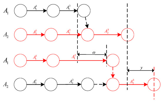
Figure 2.
Schematic diagram of dynamic critical path changes.
It can be easily inferred that when the disturbance magnitude of task exactly fills its free slack time, resulting in task and task being finished simultaneously, there will be exactly two critical paths ( and ) at this moment. As the disturbance magnitude of task further increases, task remains a critical path. This will lead to delays in the critical task node, and there is a linear positive correlation between them, expressed as follows:
Here, and are the finish times of tasks and in the plan. It can be seen that when the critical path remains unchanged, there is a positive correlation between the disturbance magnitude and the output, and the output is easy to calculate. When the critical path changes, the variation law of the structure can be easily observed in this example due to the small number of tasks. However, in the case of a large-scale (task) scenario, it is difficult for manual observation to identify such changes. Therefore, if we can grasp the changing conditions and laws of the critical path, accurate calculation can be easily achieved.
Therefore, firstly, by analyzing the effectiveness of task control, we reduce the dimensionality of the decision variables. Secondly, through a study of the critical path structure, we construct a “Critical Path Transition Tree” to achieve precise computation. This approach allows us to simultaneously improve both computational accuracy and timeliness.
In the following sections, we will, respectively, discuss the effectiveness of controllable tasks and the Critical Path Transition Tree.
- (1)
- Effectiveness of Controllable Tasks
When a disturbance occurs, not all tasks are available for control; they must first satisfy the conditions for task controllability and task state, as described in the preceding section on control constraints. However, even among these eligible tasks, applying control to every one of them will not necessarily produce the desired effect; that is, shortening the duration of certain controllable tasks may not change the system output.
Therefore, we further classify controllable tasks into two types: effective controllable tasks and ineffective controllable tasks. Consider a task at time t that is eligible for control (i.e., for which and ). If, at time t, a decrease in its duration (while holding all other task durations constant) causes the output to also decrease, then the two are positively correlated:
Then, the task is defined as an effective controllable task. Conversely, if a decrease in the task duration results in no change to the output , it is defined as an ineffective controllable task.
Theorem 1.
For a controllable task (a task that satisfies and ), if it is a task on the critical path, then when the delay amount of this task does not change the critical path, the delay amount of this task is equal to the output of the critical task node:
Proof:
According to the definition of slack time in network planning, it can be easily inferred that a task can only affect the output (i.e., the start time of critical task nodes), if its slack time is zero. Definition of the critical path: A set of tasks that start from the global start node S, end at the global end node F, where adjacent tasks have collaborative relationships, and all tasks have zero slack time is referred to as the critical path. Based on the definition of the critical path, it can be concluded that a controllable task on the critical path constitutes a sufficient condition for an effectively controllable task. This completes the proof. □
However, the aforementioned formula is conditional. The condition is that the critical path of the network plan does not change due to the occurrence of the disturbance . When the critical path changes, the portion of the disturbance magnitude corresponding to the change will not become the system output; instead, it will be converted into the slack time of the relevant node. Therefore, the relational expression in Figure 2 (discussed above) is as follows:
Unlike small-scale network planning diagrams, where there is generally only one critical path, large-scale cluster missions may involve multiple critical paths. For this reason, we use the Breadth-First Search (BFS) algorithm to identify all critical paths in the network planning diagram. Therefore, we first present the pseudocode for solving critical paths below, as shown in Algorithm 2.
| Algorithm 2: Breadth-First Search algorithm for critical path identifying |
| Function: Breadth-First Search (task ) Input: Global start node S, ends at the global end node F The set of tasks with zero slack time Set of successor tasks |
| Output: Set of critical path |
| 1. Initialization: Create a critical path set and a critical path queue ; 2. Breadth-First Search (task S): 3. Add to critical path queue ; 4. if current task == F: 5. return ; 6. for : 7. if : 8. Breadth-First Search (task ); 9. Add to ; 10. return |
For large-scale problems, the dependency relationships between tasks are highly complex, and task durations change dynamically during execution. This leads to dynamic changes in the critical path, making it difficult to derive an analytical mathematical expression and challenging to solve precisely. Therefore, we must conduct an in-depth study of how the critical path changes.
- (2)
- Critical Path Transition Tree
To study how the critical path changes dynamically, we define the reverse slack time: If a task starts a certain amount of time earlier and this action causes the current critical path to change, then this amount of time is called the task’s reverse slack time.
Let the tasks on the critical path that are in the ‘not started’ state be arranged in chronological order of their start times to form the critical path task set . Here, , and the final critical task node is .
Theorem 2:
Let task
on the critical path be the i-th task
of the critical path (where ), i.e., , and let its backward slack time be . Then, the backward slack time
of task is equal to the minimum value of the free slack time of its non-critical immediate predecessor tasks and the backward slack time of its immediate successor critical tasks, i.e.,
Proof:
Firstly, it can be observed that the above formula is a recursive formula: the backward slack time of the first task depends on , and the backward slack time of the second task depends on . Therefore, we first analyze the last task : since the immediate successor of the last task is the globally terminal node F—a manually added virtual node with a task duration of 0—the backward slack time of this task is equal to the minimum value of the free slack time among its non-critical immediate predecessor tasks:
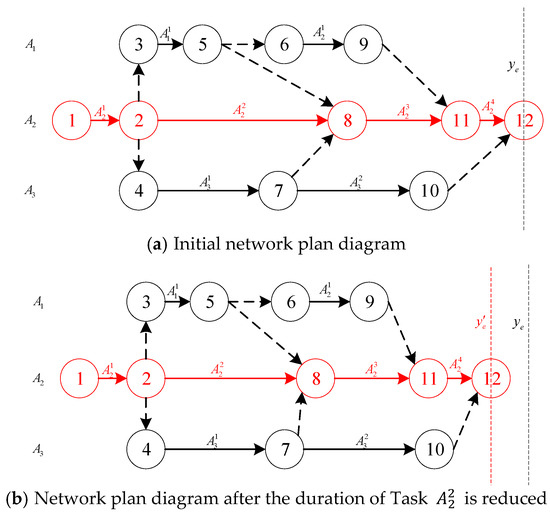
Taking Figure 3a as an example, the set of critical path tasks is . In this case, n = 4, and is ; thus,
Figure 3.
Schematic diagram for calculating reverse slack time.
Next, we analyze the second-to-last task : The early start of this task causes its immediate successor task to also start earlier by the same amount of time. Consequently, three scenarios may arise as follows:
- 1.
- When the early start time of task is exactly equal to , task mn will just change the critical path;
- 2.
- When the early start time of task is less than , but the task itself changes the critical path;
- 3.
- When the early start time of task is greater than , since the critical path has already changed when the early start time equals , any further advancement will be meaningless. According to Theorem 1, this task will no longer be an effectively controllable task.
From the above analysis, it can be concluded that
Taking Figure 3b as an example, when the duration of task is reduced, the start times of both task and task are advanced. Therefore, when considering the backward slack time of task , it is also necessary to take into account the backward slack time of task , i.e.,
It can be easily proven by mathematical induction that the backward slack time of task is equal to the minimum value of the free slack time of its non-critical immediate predecessor tasks and the backward slack time of its immediate successor critical tasks. Moreover, this conclusion also holds for the initial term where i = n. This completes the proof. □
Let the early start time for task (the i-th task mi on the critical path) be Then, this early start time is equal to the control variable for this task (where a shortened duration is represented by a negative value) plus the early start time of its immediate successor task; that is
The critical condition for a change in the critical path is the existence of a task on the critical path for which its time advancement is exactly equal to its reverse slack time; that is
Therefore, a given critical path corresponds to a certain anti-disturbance capability, and when the critical path changes, it then corresponds to a different capability. Thus, eliminating a disturbance is equivalent to “dispatching” the error, with each new critical path “receiving” the remaining error, until it is fully eliminated. However, different control strategies lead to different outcomes in how the critical path changes, consume different amounts of resources, and eliminate different amounts of error. For this reason, a “Critical Path Transition Tree” can be constructed, as shown in Figure 4.
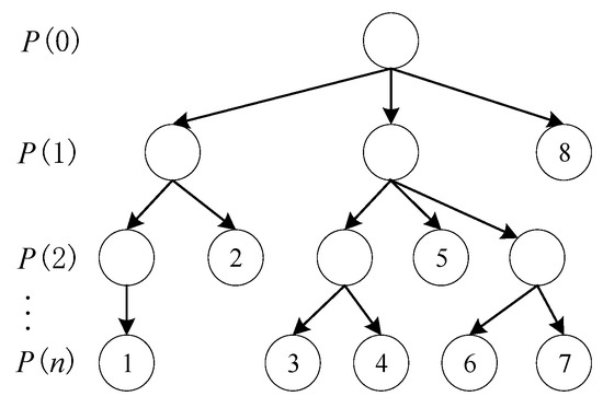
Figure 4.
The Critical Path Transition Tree.
Let us define a “stage” for each change in the critical path, where represents the state after the critical path has changed i times (i.e., it is in stage i). When a disturbance first occurs, the current critical path is the initial critical path, designated as .
At this point, the control system must, according to the critical path change conditions, find all strategies that result in a transition from . Then, for each strategy, it evaluates the relationship between the time advancement of the final critical node and the output deviation. If the time advancement is greater than or equal to the output deviation (), it signifies that the disturbance can be eliminated under this new critical path.
If the time advancement is less than the output deviation, the disturbance has not been fully eliminated. The system must then continue to “receive the order” with the next critical path, finding all strategies for the subsequent transition and re-evaluating, until the “dispatched” disturbance is completely absorbed.
When a strategy is found that can eliminate the disturbance, its specific control variables and corresponding objective function value are calculated. After traversing the entire “Critical Path Transition Tree,” each leaf node (representing a feasible solution) is compared, and the optimal control strategy is selected. A flowchart of this entire control strategy solution process is shown in Figure 5.
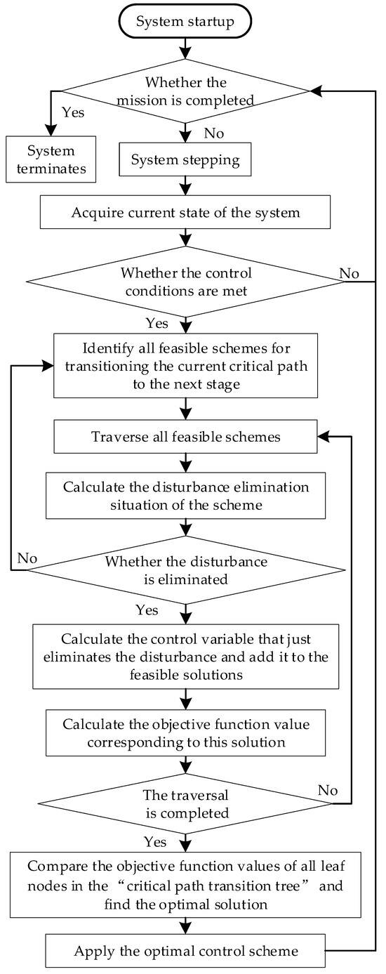
Figure 5.
Algorithm solution block diagram.
3. Results
To validate the effectiveness of the control strategy, we constructed three task scenarios, i.e., three network plans with different structures. We then applied normally distributed disturbances to each task and conducted repeated experiments, which showed favorable control performance.
In order to more intuitively demonstrate the complete mission scenario, the process of dynamic structural changes, and the effects of the control strategy, we select one of these task scenarios for a detailed analysis. We deliberately introduce several typical disturbance values to showcase three situations: (1) a disturbance that does not delay the critical node (the critical path remains unchanged), (2) a disturbance that causes a delay exactly at the threshold of changing the critical path, and (3) a disturbance that delays the critical node, causing the critical path to change and postpone the node. We then solve for the control variables to demonstrate the full scope of the “Critical Path Transition Tree” algorithm.
We constructed a collaborative multi-agent mission to be jointly completed by 15 executors (15 UAVs). On the left side of the figure is the red force, the offensive side, which includes two refueling drones, three communication drones, two reconnaissance drones, two jamming drones, and six strike drones; on the right side of the figure is the blue force, which has multiple key targets. The aviation cluster mission of the red force is to strike the key targets of the blue force, as shown in Figure 6 below. Through the Work Breakdown Structure (WBS) technique [31], the mission was decomposed into multiple tasks that each executor is required to perform, and the collaborative relationships existing between these tasks were identified. The entire plan comprises a total of 119 subtasks, as shown in Appendix Table A1. A UAV inherently has a variety of parameters; however, this paper focuses primarily on mission scheduling. Therefore, only brief information about the UAVs—including their types, flight performance, and fuel consumption rates—is provided herein. The basic parameters of the speed and fuel consumption rate for each UAV are presented in Table 1. UAVs listed in the same row (e.g., E/F) indicate models with identical specifications and performance. Specifically, UAVs B, C, and D are assigned to communication tasks; UAVs A and G to reconnaissance tasks; UAVs J, M, K, N, I, and P to ground strike tasks targeting different objectives; UAVs H and L to jamming tasks; and UAVs E and F to tanker tasks (i.e., in-flight refueling provision). The UAVs capable of receiving in-flight refueling are B, C, D, I, J, K, L, M, N, and P, with a refueling rate of 600 kg·min−1.
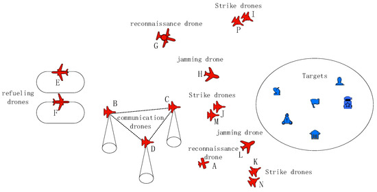
Figure 6.
Schematic diagram of the experimental scenario.

Table 1.
UAV flight and fuel consumption performance parameters.
Based on the above parameters, the network schedule plan was formulated and is presented in Figure 7, with all task information provided in Appendix Table A1. In the network schedule plan diagram, arrows represent tasks, marked with task codes (e.g., A1, B2); circles represent nodes, indicating the start or end time of the corresponding task; dashed lines represent dummy tasks, used to characterize task dependencies; red arrows denote the critical path, while blue-colored tasks represent the controllable tasks identified by the system at the current moment; and the gray vertical line represents the current moment. As time progresses, the status of each task changes according to actual conditions, and tasks that have been completed are displayed in gray.
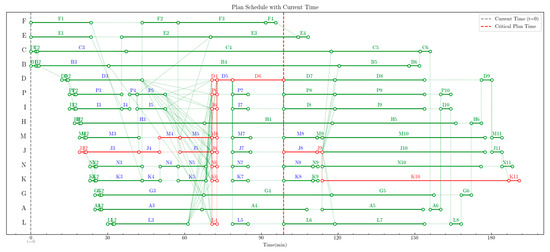
Figure 7.
Initial plan diagram.
In this plan, the controllable tasks are as follows: A3, B3, C3, D3, D5, E1, F1, G3, H3, I3, I4, I5, I7, P3, P4, P5, P7, J3, J4, J5, J7, J8, M3, M4, M5, M7, M8, L3, L5, K3, K4, K5, K7, K8, N3, N4, N5, N7, and N8, which are indicated in blue font; the critical task node is J8, with a scheduled start time of 98.8 min. This indicates that task J8 must start at this exact moment, and this time point is marked with a red dashed line. If during the task execution process, the scheduled start time of J8 is delayed beyond 98.8 min due to the postponement of its preceding tasks, it is deemed a delay, and control measures need to be implemented.
We then proceed to discuss the fuel capacity of UAVs. For non-refuellable UAVs (A, G, H), fuel consumption calculation is relatively straightforward—only the fuel consumption of their respective subtasks and hovering fuel need to be calculated. The calculation results show that their fuel capacity requirements are all satisfied, so detailed elaboration is omitted herein. For refuellable UAVs, their refueling planning is more complex. It is necessary to consider not only the refueling amount of each UAV (which determines the refueling duration and thus affects the start time of each task for each UAV) but also the refueling sequence of different receiver UAVs under the condition of limited refueling aircraft. The final refueling planning results are presented in Table 2.
Table 2.
UAV fuel usage plan.
To demonstrate the impact of disturbances on the plan, we artificially set several typical disturbances, which correspond to three scenarios: (1) the disturbance does not cause critical node delay (critical path remains unchanged); (2) the disturbance just causes critical node delay (critical path changes exactly); and (3) the disturbance causes critical node delay (critical path change leads to critical node postponement). The disturbances we set are as follows: task E1 is delayed by 10 min in its start time; task N1 is extended by 9.3 min in its completion time; and task K3 is extended by 5 min in its completion time.
Before the application of disturbances (i.e., in the planned state), the start times of all subtasks are presented in Table A1. Among these tasks, task E1 is scheduled to start at 0 min and end at 23.5 min; and task N1 is scheduled to start at 23 min and end at 25 min. At this stage, the critical paths consist of a total of 16 paths, with the representative path expressed as follows: J1-J2-J3-J4-M4-[J5, M5]-[D4, P6, I6, M6, J6, N6, K6, L4]-D5-D6-J8-K10-K11.
After disturbances occur in task E1 and task N1, the network schedule at time t = 34 is shown in Figure 8. At this moment, the actual start time of task E1 is 10 min, and its actual end time is 33.5 min; and the actual start time of task N1 remains 23 min, while its actual end time is extended to 34.3 min.
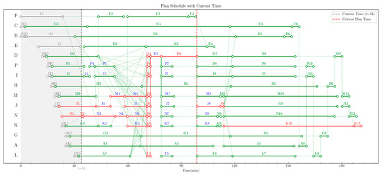
Figure 8.
Schedule diagram where disturbances occur without delaying critical task nodes.
As observed in Figure 8, task E has moved from the second row in Figure 7 to the fourth row in Figure 8, with the start time of task E1 also delayed; the delay of task N1 has caused task N1 and task N3 to be successively delayed. At this point, the scheduled end time of task N3 exactly coincides with the scheduled start time of task N4, leading to an exact change in the critical path. The critical paths now become two categories:
J3-J4-M4-[J5, M5]-[D4, P6, I6, M6, J6, N6, K6, L4]-D5-D6-J8-K10-K11;
N1-N2-N3-N4-[N5, K5]-[D4, P6, I6, M6, J6, N6, K6, L4]-D5-D6-J8-K10-K11.
However, the start time of task J8 remains 98.8 min, which still coincides with the red dashed line. This indicates that the disturbance has no impact on the critical node.
As shown in Figure 9, with the execution of tasks, at time t = 49, task K3 is delayed by 5 min. Its original schedule—scheduled to start at 25.5 min and end at 43.5 min—has changed to an actual start time of 25.5 min and an actual end time of 48.5 min. At this point, the critical path changes again, and the new critical path is as follows: K4-N4-[N5, K5]-[D4, P6, I6, M6, J6, N6, K6, L4]-D5-D6-J8-K10-K11. It can be observed that the start time of task J8 is now 101.5 min, meaning the critical task node is delayed by 2.7 min, and its start time is postponed relative to the red dashed line.
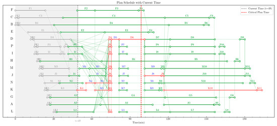
Figure 9.
Diagram of disturbances causing delays in critical task nodes.
In practice, between t = 46 and t = 49, the system had already detected the postponement of the critical task node, but no control was implemented. This is because the control conditions were not satisfied at that time—the delayed task K3 had not yet been completed. At time t = 49, the control conditions are met as follows:
- There is a disturbance at the current moment;
- All delayed tasks have been completed by the current moment;
- A delayed task is exactly completed at the current moment.
Thus, the control system begins to solve for the control strategy.
The time delay not only prevents the critical task node J8 from being executed on schedule but also results in insufficient fuel for UAV J and UAV M. At this point, the set of controllable tasks that meet the control conditions is M4, M5, J5, N4, N5, K5, D5, P7, I7, M7, J7, N7, K7, L5, M8, J8, N8, and K8, which are represented by all blue-font tasks in Figure 9. Based on the effectiveness of controllable tasks, the currently effective controllable tasks are calculated as [N4, N5, K5, D5]. This significantly reduces the decision-making dimension and improves the convergence speed of the algorithm.
At this stage, the algorithm starts to construct the “Critical Path Transition Tree”. Since the duration of the delay is exactly equal to the backward slack time of task N4, the critical path does not transition. The 2.7 min “task delay (referred to as ‘order dumping’ herein)” in the output can be fully “absorbed (referred to as ‘order receiving’ herein)” by the current critical path. Therefore, the algorithm proceeds to distribute the “order dumping” to each effective controllable task under the current path, with each effective controllable task undertaking the “order receiving”. At this point, each controllable task is subject to certain control constraints; for example, shortening tasks D5, N5, and K5 is constrained by both the flight speed limit and the UAV fuel capacity limit.
The final computed solution is as follows: the duration of refueling task N4 is shortened by 2.7 min. This means the amount of fuel for UAV N is changed from the originally planned 4200 kg to 2580 kg. The resulting network schedule after this control action is shown in Figure 10. With this solution, the system’s remaining anti-disturbance capability is 8.8 min, which is the maximum value among the 316 calculated control strategies.
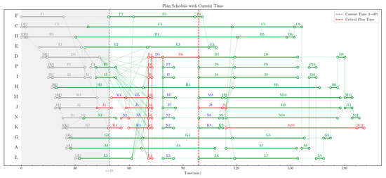
Figure 10.
Control system eliminating disturbances.
In the aforementioned experiments, to more intuitively demonstrate the dynamic change process of the network structure and the effect of control, we artificially set three typical disturbance magnitudes. These magnitudes correspond to three scenarios for solving the control quantity: (1) a disturbance that does not delay the critical node (the critical path remains unchanged), (2) a disturbance that causes a delay exactly at the threshold of changing the critical path, and (3) a disturbance that delays the critical node, causing the critical path to change and postpone the node.
Next, to compare the accuracy and timeliness of the “Critical Path Transition Tree” algorithm with those of traditional RCPSP model algorithms, we designed the following experiment: random Gaussian disturbances are applied to the 119 subtasks included in this mission scenario. The probability of generating disturbances is set to 0.5, and the generated disturbance values follow a normal Gaussian distribution. The task duration disturbance variances of each subtask are provided in Appendix 4. It should be noted that Gaussian disturbances may either extend or shorten task durations; however, the actual mission requirements dictate that changes to the plan should be minimized as much as possible. Therefore, disturbances that would shorten task durations are treated as having no shortening effect. In practical terms, this means that after a UAV completes its preceding subtasks ahead of schedule, it does not immediately execute the next subtask but hovers in place until the scheduled start time of the next subtask before executing it.
We conducted 100 Monte Carlo simulations to compare the “Critical Path Transition Tree” algorithm with the adaptive differential evolution algorithm [32] in three aspects: average algorithm accuracy (accuracy: the absolute value of the output y after control is applied), average algorithm time consumption (time consumption: the time taken for the algorithm to solve a control strategy once), and task success rate (after control is implemented, key task nodes are executed on time). Since intelligent optimization algorithms approach the global optimal solution through random search, the algorithm accuracy is not zero. In handling the task success rate, we relaxed the definition of “on-time” task execution by 0.8 min (i.e., execution within ±0.8 min of the planned time is considered on-time). The final experimental results are shown in Table 3.
Table 3.
Results of comparative experiments on different algorithms.
4. Conclusions
For the problem of resource-constrained project scheduling and control, this paper proposes a precise control method based on a “Critical Path Transition Tree.” By analyzing the effectiveness of controllable tasks, we define “reverse slack time” to precisely identify the conditions under which the critical path will change. Furthermore, for effective tasks on the critical path, the required reduction in duration equals the delay, which locally solves the difficult inverse mapping problem of the recursive formula. The “Critical Path Transition Tree” then allows the global, complex problem to be decomposed into multiple simpler, local problems. This transforms the dynamically changing network plan from a “black box” to a “gray box,” enabling precise control. Finally, simulation experiments were conducted, verifying that the algorithm’s solution time is 1–2 s, which demonstrates its strong timeliness for real-time applications. This method is not only applicable to aviation cluster missions but also to all schedule planning problems that consider time disturbances. The differences between different problem scenarios lie in the forms of resources and the subtasks decomposed by WBS. We hope the proposed method can provide valuable insights for future research, as unmanned real-time disturbance control under resource constraints has become a critical problem to solve with the expanding scale of modern production and logistics.
Meanwhile, this paper still has several limitations that can be addressed and improved in future research, specifically the following: overly strict control conditions, limited control measures, and a single type of disturbance variable.
- (1)
- Overly strict control conditions. The control system established in this paper intervenes in control only when three conditions are simultaneously satisfied, and control can only be implemented when all currently delayed tasks are completed. When the task scale is larger (with hundreds of UAVs) and multiple disturbances occur simultaneously, it may become difficult for the system to meet the control timing requirements, resulting in delays in control intervention. Future research can draw on the EVM, set multiple checkpoints for key tasks, and establish a disturbance prediction model to achieve proactive prediction of potential disturbances. This would enable estimating the disturbance magnitude as soon as a disturbance emerges and conducting more timely control interventions.
- (2)
- Limited control measures. The control measure proposed in this paper focuses on regulating task durations (essentially, the amount of fuel refueled also controls the refueling duration). However, in practical applications, more diverse control measures may be adopted to further eliminate delay disturbances, such as simplifying task processes (by removing subtasks) and dynamically modifying the dependency relationships among subtasks. Therefore, future research can explore incorporating such more diverse control variables into the scheduling framework.
- (3)
- A single type of disturbance variable. This paper only considers time disturbances and does not account for disturbances in the number of UAVs (e.g., a UAV being forced to land due to a malfunction after takeoff). In practical missions, changes in the number of UAVs may lead to dynamic modifications of strike targets, the formulation of entirely new tasks, or even the cancellation of tasks. This requires constructing a UAV quantity-target mapping model, which falls within the scope of dynamic task planning.
Author Contributions
Conceptualization, Y.S. and Q.S.; software, Y.S. and Q.S.; formal analysis, B.W.; investigation, J.L. and Q.S.; resources, Y.S. and Y.W.; data curation, Y.W. and D.W.; writing—original draft preparation, Y.S. and Q.S.; writing—review and editing, J.Z. and Y.W.; visualization, B.W. and J.Z.; supervision, J.L. and Y.S.; project administration, Y.S. and J.L.; funding acquisition, D.W. and Y.S. Y.S. and Q.S. contributed equally to this work. All authors have read and agreed to the published version of the manuscript.
Funding
This research was funded by the National Social Science Fund of China (Grant No. 2022-SKJJ-B-051).
Data Availability Statement
The data presented in this study is available on request from the corresponding author.
Conflicts of Interest
The authors declare no conflicts of interest.
Appendix A
Table A1.
Formation task list based on Work Breakdown Structure.
Table A1.
Formation task list based on Work Breakdown Structure.
| Task Code | Planned Task Duration/min | Duration Variance | Predecessor Task | Planned Start Time/min | Planned Finish Time/min |
|---|---|---|---|---|---|
| A1 | 2.0 | 0.1 | START | 25.0 | 27.0 |
| A2 | 0.5 | 0.1 | A1 | 27.0 | 27.5 |
| A3 | 39.3 | 4.0 | A2 | 27.5 | 66.8 |
| A4 | 50.0 | 10.0 | A3 | 66.8 | 107.8 |
| A5 | 39.3 | 5.0 | A4/J9 | 113.9 | 153.2 |
| A6 | 4.0 | 0.10 | A5/C6 | 156.1 | 160.1 |
| B1 | 2.0 | 0.1 | START | 0 | 2.0 |
| B2 | 0.5 | 0.05 | B1/C2 | 2.5 | 3.0 |
| B3 | 27.4 | 3.0 | B2 | 3.0 | 30.4 |
| B4 | 90.0 | 10.0 | B3 | 30.4 | 120.4 |
| B5 | 27.4 | 5.0 | B4/J9 | 120.4 | 147.8 |
| B6 | 4.0 | 0.1 | B5 | 147.8 | 151.8 |
| C1 | 2.0 | 0.1 | START | 0 | 2.0 |
| C2 | 0.5 | 0.1 | C1 | 2.0 | 2.5 |
| C3 | 34.8 | 4.0 | C2 | 2.5 | 37.3 |
| C4 | 90.0 | 10.0 | C3 | 37.3 | 117.3 |
| C5 | 34.8 | 5.0 | C4/J9 | 117.3 | 152.1 |
| C6 | 4.0 | 0.1 | C5/B6 | 152.1 | 156.1 |
| D1 | 2.0 | 0.1 | START | 12.0 | 14.0 |
| D2 | 0.5 | 0.1 | D1/B2 | 14.0 | 14.5 |
| D3 | 28.9 | 6.0 | D2 | 14.5 | 43.4 |
| D4 | 2.0 | 0.1 | D3/I5/J5/K5/L3 | 70.7 | 72.7 |
| D5 | 6.1 | 0.1 | D4/I6/J6/K6/L4/A3/G3/H3 | 72.7 | 78.8 |
| D6 | 20.0 | 2.0 | D5 | 78.8 | 98.8 |
| D7 | 20.0 | 3.0 | D6 | 98.8 | 118.8 |
| D8 | 55.0 | 7.0 | D7/J9 | 118.8 | 153.8 |
| D9 | 4.0 | 0.1 | D8/H6 | 176.1 | 180.1 |
| E1 | 23.5 | 5.0 | START | 0 | 23.5 |
| E2 | 50.0 | 2.0 | E1/I3 | 35.5 | 70.2 |
| E3 | 34.2 | 5.0 | E2/I4/J4 | 70.2 | 104.4 |
| E4 | 4.0 | 0.1 | E3/F4 | 104.4 | 108.4 |
| F1 | 23.5 | 0 | START | 0 | 23.5 |
| F2 | 50.0 | 2.0 | F1/K3 | 43.5 | 57.5 |
| F3 | 34.2 | 2.0 | F2/K4 | 57.5 | 91.7 |
| F4 | 4.0 | 0.1 | F3 | 91.7 | 95.7 |
| G1 | 2.0 | 0.1 | START | 25.0 | 27.0 |
| G2 | 0.5 | 0.1 | G1 | 27.0 | 27.5 |
| G3 | 40.0 | 5.0 | G2 | 27.5 | 67.5 |
| G4 | 50.0 | 5.0 | G3/B3 | 67.5 | 117.5 |
| G5 | 40.0 | 3.0 | G4/J9 | 117.5 | 157.5 |
| G6 | 4.0 | 0.1 | G5/L8 | 168.1 | 172.1 |
| H1 | 2.0 | 0.1 | START | 17.0 | 19.0 |
| H2 | 0.5 | 0.1 | H1 | 19.0 | 19.5 |
| H3 | 48.3 | 5.0 | H2 | 19.5 | 67.8 |
| H4 | 50.0 | 5.0 | H3 | 67.8 | 117.8 |
| H5 | 48.3 | 3.0 | H4/J9 | 117.8 | 166.1 |
| H6 | 4.0 | 0.1 | H5/G6 | 172.1 | 176.1 |
| I1 | 2.0 | 0.1 | START | 15.0 | 17.0 |
| I2 | 0.5 | 0.1 | I1/D2 | 160.1 | 164.1 |
| I3 | 18.0 | 2.0 | I2 | 17.0 | 17.5 |
| I4 | 9.0 | 0.5 | I3/E1 | 17.5 | 35.5 |
| I5 | 10.9 | 0.5 | I4 | 35.5 | 38.5 |
| I6 | 2.0 | 0.1 | D3/I5/J5/K5/L3 | 41.5 | 52.4 |
| I7 | 6.1 | 0.2 | I6/D5 | 70.7 | 72.7 |
| I8 | 20.0 | 1.2 | I7/D6 | 78.8 | 84.9 |
| I9 | 35.0 | 3.5 | I8/J9 | 98.8 | 118.8 |
| I10 | 4.0 | 0.1 | I9/A6 | 118.8 | 153.8 |
| J1 | 2.0 | 0.1 | START | 19.0 | 21.0 |
| J2 | 0.5 | 0.1 | J1 | 113.9 | 177.4 |
| J3 | 20.7 | 0.8 | J2 | 180.1 | 184.1 |
| J4 | 8.0 | 1.0 | J3/P4 | 21.0 | 21.5 |
| J5 | 12.5 | 0.8 | J4 | 21.5 | 42.2 |
| J6 | 2.0 | 0.1 | D3/I5/J5/K5/L3 | 42.2 | 50.2 |
| J7 | 7.0 | 1.0 | J6/D5 | 58.2 | 70.7 |
| J8 | 13.1 | 1.2 | J7/D6 | 70.7 | 72.7 |
| J9 | 2.0 | 0.5 | J8 | 78.8 | 85.8 |
| J10 | 63.5 | 10.0 | J9 | 98.8 | 111.9 |
| J11 | 4.0 | 0.1 | J10/D9 | 111.9 | 113.9 |
| K1 | 2.0 | 0.1 | START | 23.0 | 25.0 |
| K2 | 0.5 | 0.1 | K1/J2 | 113.9 | 186.8 |
| K3 | 18.0 | 4.1 | K2 | 186.8 | 190.8 |
| K4 | 7.0 | 1.0 | K3/F1 | 25.0 | 25.5 |
| K5 | 10.9 | 0.6 | K4 | 25.5 | 43.5 |
| K6 | 2.0 | 0.1 | D3/I5/J5/K5/L3 | 43.5 | 50.5 |
| K7 | 6.1 | 0.8 | K6/D5 | 57.5 | 68.4 |
| K8 | 11.4 | 1.0 | K7/D6 | 70.7 | 72.7 |
| K9 | 2.0 | 0.3 | K8 | 78.8 | 84.9 |
| K10 | 62.0 | 6.0 | K9/J9 | 98.8 | 110.2 |
| K11 | 4.0 | 0.1 | K10/J11 | 110.2 | 112.2 |
| L1 | 2.0 | 0.1 | START | 30.0 | 32.0 |
| L2 | 0.5 | 0.1 | L1 | 32.0 | 32.5 |
| L3 | 28.9 | 5.2 | L2 | 32.5 | 61.4 |
| L4 | 2.0 | 0.1 | D3/I5/J5/K5/L3 | 70.7 | 72.7 |
| L5 | 6.1 | 0.2 | L4/D5 | 78.8 | 84.9 |
| L6 | 20.0 | 2.0 | L5/D6 | 98.8 | 118.8 |
| L7 | 35.0 | 1.0 | L6/J9 | 118.8 | 153.8 |
| L8 | 4.0 | 0.10 | L7/I10 | 164.1 | 168.1 |
| M1 | 2.0 | 0.1 | START | 19.0 | 21.0 |
| M2 | 0.5 | 0.1 | M1 | 113.9 | 177.4 |
| M3 | 20.7 | 2.0 | M2 | 180.1 | 184.1 |
| M4 | 8.0 | 1.00 | M3/J4 | 21.0 | 21.5 |
| M5 | 12.5 | 0.5 | M4 | 21.5 | 42.2 |
| M6 | 2.0 | 0.1 | D3/I5/J5/K5/L3 | 50.2 | 58.2 |
| M7 | 7.0 | 0.3 | M6/D5 | 58.2 | 70.7 |
| M8 | 13.1 | 0.9 | M7/D6 | 70.7 | 72.7 |
| M9 | 2.0 | 0.2 | M8 | 78.8 | 85.8 |
| M10 | 63.5 | 5.0 | M9 | 98.8 | 111.9 |
| M11 | 4.0 | 0.1 | M10/D9 | 111.9 | 113.9 |
| N1 | 2.0 | 0.1 | START | 23.0 | 25.0 |
| N2 | 0.5 | 0.1 | N1/J2 | 113.9 | 175.9 |
| N3 | 18.0 | 0.6 | N2 | 184.1 | 188.1 |
| N4 | 7.0 | 1.0 | N3/K4 | 25.0 | 25.5 |
| N5 | 10.9 | 0.5 | N4 | 25.5 | 43.5 |
| N6 | 2.0 | 0.1 | D3/I5/J5/N5/L3 | 50.5 | 57.5 |
| N7 | 6.1 | 0.3 | N6/D5 | 57.5 | 68.4 |
| N8 | 11.4 | 0 | N7/D6 | 70.7 | 72.7 |
| N9 | 2.0 | 0.3 | N8 | 78.8 | 84.9 |
| N10 | 62.0 | 8.2 | N9/J9 | 98.8 | 110.2 |
| N11 | 4.0 | 0.1 | N10/J11 | 110.2 | 112.2 |
| P1 | 2.0 | 0 | START | 15.0 | 17.0 |
| P2 | 0.5 | 0 | P1/D2 | 160.1 | 164.1 |
| P3 | 18.0 | 2.0 | P2 | 17.0 | 17.5 |
| P4 | 9.0 | 0.2 | P3/I4 | 17.5 | 35.5 |
| P5 | 10.9 | 0.5 | P4 | 38.5 | 41.5 |
| P6 | 2.0 | 0.1 | D3/P5/J5/K5/L3 | 41.5 | 52.4 |
| P7 | 6.1 | 1.0 | P6/D5 | 70.7 | 72.7 |
| P8 | 20.0 | 3.0 | P7/D6 | 78.8 | 84.9 |
| P9 | 35.0 | 2.3 | P8/J9 | 98.8 | 118.8 |
| P10 | 4.0 | 0.10 | P9/A6 | 118.8 | 153.8 |
References
- Chen, F.; Wang, Z.; Tian, X.L. A production schedule evaluation method based on program evaluation and review technique. J. Ordnance Equip. Eng. 2016, 37, 177–180. [Google Scholar]
- Ma, G.F.; Chen, Q. Study on project scheduling management. Shanghai Manag. Sci. 2006, 28, 70–74. [Google Scholar]
- Sadri, S.; Ghomi, S.M.T.F.; Deghghanian, A. Analysis of a time-cost trade-off in a resource-constrained GERT project scheduling problem using the Markov decision process. Ann. Oper. Res. 2024, 338, 535–568. [Google Scholar] [CrossRef]
- Wang, L.; Liu, H.; Xia, M.; Wang, Y.; Li, M. A machine learning based EMA-DCPM algorithm for production scheduling. Sci. Rep. 2024, 14, 20810. [Google Scholar] [CrossRef] [PubMed]
- Davis, E.W. Project scheduling under resource constraints: Historical review and categorization of procedures. AIIE Trans. 1973, 5, 297–313. [Google Scholar] [CrossRef]
- Levchuk, G.M.; Levchuk, Y.N.; Luo, J.; Pattipati, K.R.; Kleinman, D.L. Normative design of organizations. I. mission planning. IEEE Trans. Syst. Man Cybern.–Part A Syst. Hum. 2002, 32, 346–359. [Google Scholar] [CrossRef]
- Machado Lf Paternina, C.D.; Velez, J. An adaptative bacterial foraging optimization algorithm for solving the MRCPSP with discounted cash flows. Top 2022, 30, 221–248. [Google Scholar] [CrossRef]
- Hu, M.; Zhou, M.; Zhang, Z.; Zhang, L.; Li, Y. A novel disjunctive-graph-based meta-heuristic approach for multi-objective resource-constrained project scheduling problem with multi-skilled staff. Swarm Evol. Comput. 2025, 95, 101939. [Google Scholar] [CrossRef]
- Peng, W.L.; Lin, X.J.; Li, H.T. Critical chain based Proactive-Reactive scheduling for Resource-Constrained project scheduling under uncertainty. Expert Syst. Appl. 2023, 214, 119188. [Google Scholar] [CrossRef]
- Passlanneau, A.; Bendotti, P.; Brunodindrigo, L. Exact and heuristic methods for Anchor-Robust and Adjustable-Robust RCPSP. Ann. Oper. Res. 2024, 337, 649–682. [Google Scholar] [CrossRef]
- Peng, W.L.; Lin, X.J. A Dynamic Reactive Scheduling Method for the Resource Constrained Project Scheduling Problem. Chin. J. Manag. Sci. 2025, 33, 200–209. [Google Scholar]
- Guo, W.K.; Vanhoucks, M.; Coelho, J. Comparison of two problem transformation-based methods in detecting the best performing branch-and-bound procedures for the RCPSP. Expert Syst. Appl. 2025, 281, 127383. [Google Scholar] [CrossRef]
- Melo, L.V.; Queiroz, T.A. Integer Linear Programming Formulations for the RCPSP considering Multi-Skill, Multi-Mode, and Minimum and Maximum Time Lags. IEEE Lat. Am. Trans. 2021, 19, 5–16. [Google Scholar] [CrossRef]
- Carvin, B.; Bellenguez, O.; Massonnet, G. Tabu search for a multi-mode RCPSP with generalized precedence sequence-dependent setup time. Comput. Ind. Eng 2025, 111142. [Google Scholar] [CrossRef]
- Cai, H.X.; Bian, Y.Q.; Liu, L.L. Deep reinforcement learning for solving resource constrained project scheduling problems with resource disruptions. Robot. Comput.-Integr. Manuf. 2024, 85, 102628. [Google Scholar] [CrossRef]
- Xue, W.R. Research on Project Schedule Management Oriented to Collaborative Construction. Ph.D. Thesis, Harbin Institute of Technology, Harbin, China, 2015; pp. 1–45. [Google Scholar]
- Guan, Y.; Du, X.L. Research on production planning management in supply chain management environment. Mod. Ind. Econ. Informationization 2023, 13, 236–238. [Google Scholar]
- Yang, X.J. Research on Production Schedule Control of Aerospace Products Based on Multi-Level Earned Value Method. Ph.D. Thesis, Harbin Engineering University, Harbin, China, 2015; pp. 1–38. [Google Scholar]
- Zhang, Y. Application of improved earned value method in cost control of road construction projects. Eng. Cost Manag. 2024, 69–75. [Google Scholar] [CrossRef]
- Li, S.M.; Hu, J.B.; Xu, S.Y.; Sun, D.J.; Wei, Z.H. Evaluation of flight plan robustness based on flight redistribution. J. Nanjing Univ. Aeronaut. Astronaut. 2023, 55, 1044–1054. [Google Scholar] [CrossRef]
- Qu, J.Y.; Wu, S.X.; Zhang, J.J. Flight delay propagation prediction based on deep learning. Mathematics 2023, 11, 494. [Google Scholar] [CrossRef]
- Wei, X.; Li, Y.; Shang, R.; Ruan, C.; Xing, J. Airport cluster delay prediction based on TS-BiLSTM-attention. Aerospace 2023, 10, 580. [Google Scholar] [CrossRef]
- Dong, B.; Peng, Z.C. Irregular flight recovery under resource restriction. Ship Electron. Eng. 2024, 44, 51–56. [Google Scholar]
- Wang, W.H.; Luan, S.C. The crucial technology research of operational plan management. Comput. Knowl. Technol. 2010, 6, 4841–4844. [Google Scholar]
- Zhang, Y.X. Research on Modeling and Optimization Method of Military Mission Plan in Uncertain Environment. Ph.D. Thesis, National University of Defense Technology, Changsha, China, 2014; pp. 1–35. [Google Scholar]
- Chen, X.J.; Qi, H.; Yang, D.S. Modeling and solution of joint operational plans with time windows. Syst. Eng-Theory Pract. 2012, 32, 1979–1985. [Google Scholar]
- Sun, P.; Chen, G.Y.; Zhang, J.Y.; Wu, J.S. Dynamic task plan adjustment model and algorithm based on battlefield emergencies. Control Decis. 2020, 35, 1052–1062. [Google Scholar]
- Wu, R.J.; Sun, P.; Sun, Y. Distributed dynamic task plan adjustment model and algorithm. Syst. Eng. Electron. 2017, 39, 322–328. [Google Scholar]
- Yang, X.M.; Yu, J.; Chen, Y.; Gao, Q.F. Design of battle management system based on workflow engine. Command Inf. Syst. Technol. 2024, 15, 21–27. [Google Scholar] [CrossRef]
- Fang, B.; Wang, Z.W.; Chen, A.; Chen, W.X. Technology for intelligent battle management. Command Inf. Syst. Technol. 2023, 14, 18–24. [Google Scholar] [CrossRef]
- Saputra, P.D.; Fansuri, M.H.; Laksmi, A.A. Development of work breakdown structure (WBS) for rapid damage runway repair (RADARR) time planning at military airbases. E3S Web Conf. 2024, 517, 05002. [Google Scholar] [CrossRef]
- Song, Q.; Zuo, J.L.; Wu, A.; Yang, R.N.; Wang, Y.; Li, L.Y. Collaborative mission schedule management method for air battle management. Acta Aeronaut. Et Astronaut. Sin. 2025, 46, 331480. (In Chinese) [Google Scholar] [CrossRef]
Disclaimer/Publisher’s Note: The statements, opinions and data contained in all publications are solely those of the individual author(s) and contributor(s) and not of MDPI and/or the editor(s). MDPI and/or the editor(s) disclaim responsibility for any injury to people or property resulting from any ideas, methods, instructions or products referred to in the content. |
© 2025 by the authors. Licensee MDPI, Basel, Switzerland. This article is an open access article distributed under the terms and conditions of the Creative Commons Attribution (CC BY) license (https://creativecommons.org/licenses/by/4.0/).