Research on the Indirect Solution Optimization Regularization Method for Ship Mechanical Excitation Force

Featured Application

The optimization regularization method proposed in this paper has achieved very good results in solving the indirect calculation problem of excitation force in the field of ships.

Abstract

Accurate identification of mechanical excitation forces is of great significance for the control of ship radiated noise and structural design. Currently, the identification of excitation forces mostly relies on indirect calculations, which suffer from ill-conditioned problems. Regularization correction is one of the main means to solve this problem. Although regularization methods have been widely developed, their application in the field of ships is relatively rare. Currently, the commonly used methods are truncation singular values and Givonov regularization methods. This paper starts from the practical application of ships and addresses the problem of poor correction effect of traditional regularization methods. Two optimized regularization methods, quasi-optimal discriminant criterion and B-spline interpolation function method, are proposed. These methods are verified through simulations and experiments. The results of the scaled model experiments show that compared with using the L-curve alone, the Q-O method reduces the regularization error by 29%, while the BL curve improves the robustness by 38% under a 15 dB noise condition.

1. Introduction

In the current engineering and technological fields, a large number of vibration problems exist in various equipment and structures. Issues such as structural safety and reliability caused by vibration have become the focus of attention. To solve vibration problems, it is first necessary to trace the source of vibration. However, in most cases, it is difficult or impossible to directly measure the vibration sources (i.e., the applied external loads) on structures in engineering practice [1].

The basic principle of dynamic load identification (or reconstruction, inversion) is to invert the dynamic excitation acting on a structural system based on the measured dynamic response of the structural system and the known dynamic characteristics of the structural system. It belongs to the second type of inverse problem in structural dynamics and is a typical source identification inverse problem in mathematics [2].

The dynamic load identification technology can be traced back to the 1970s, originating from the aviation industry, and was used to study the dynamic loads at the center of helicopter rotor hubs. So far, dynamic load identification has developed for nearly 50 years, attracting more and more scholars to engage in research in this field. Some classic algorithms and theories have also been formed, which have promoted the development of structural dynamics in the aerospace field. This technology has also been extended and applied to engineering fields such as transportation, building structures, wind resistance and disaster prevention, and health monitoring. However, its application in the marine field is relatively scarce [3]. In fact, effectively identifying the excitation force during the operation of marine mechanical equipment and the structural bearing load can effectively predict the radiated noise of ships, which is of great significance for ship noise control and acoustic design.

Dynamic load identification is a reverse solution process, and its core challenge lies in addressing the instability of the solution to this inverse problem [4]. In the field of marine engineering, the currently commonly used solutions are still in the primary stage, mainly involving methods based on Singular Value Decomposition (SVD) [5,6] and Tikhonov regularization technology [7,8,9].

In the field of marine engineering, the reason why the reverse solution of excitation force has not been fully developed might be due to the complex marine environment and unstable background noise, which makes it impossible to accurately determine the noise level and other relevant information in the data set. Therefore, only a posteriori strategies can be adopted to solve the ill-conditioned problem in the inverse problem solution. The commonly used posteriori strategies are Generalized Cross Validation (GCV) and L-curve method.

Truncated singular value decomposition (TSVD) [10,11], a classical approach for diagnosing matrix ill-conditioning, is widely used in SVD-based methods. The process begins with decomposing the original transfer function matrix through singular value decomposition (SVD). Then, singular values below a preselected threshold are set to zero, reconstructing a modified transfer matrix with a reduced condition number. Powell [12] improved this method by incorporating the coherence function analysis of excitation forces and structural responses across various frequencies, optimizing the truncation points. Meanwhile, Romano [13] proposed a fixed threshold criterion, suggesting discarding singular values below 10% of the maximum singular value. The underlying assumption is that when singular values are smaller than the secondary threshold, their removal has minimal impact on the calculation results.

In contrast to TSVD, Tikhonov regularization achieves a balance between stability and accuracy through a regularization parameter. Determining the optimal value of this parameter remains crucial. In ship engineering applications, the L-curve [14,15,16] and generalized cross-validation (GCV) [17,18] are the two dominant selection methods.

Based on the Tikhonov regularization method for solutions, the key lies in the calculation of the regularization parameter. By using the GCV method and the L-curve method to solve the regularization parameter, the essence is to balance the stability of the solution and the influence of errors. However, when the system disturbance or background noise is large, the accuracy of the two methods will also decrease. This is because the curvature feature distortion caused by noise leads to the convergence of the GCV and L-curve methods to pseudo-optimal parameters. Therefore, to solve the above problems, this paper, based on the GCV and L-curve methods, combines application and further proposes an improved quasi-optimal discrimination criterion (Q-O) and B-spline interpolation function method to seek the optimal regularization parameter:

(a)

Quasi-optimal (Q-O) refinement: Conduct grid search within the stable region of the L curve. Optimize the division of regions through Hausdorff distance to ensure stability.

(b)

Weighted B-spline Stabilization (BL-curve): Embeds residual confidence-weighted B-spline interpolation, reducing curvature calculation error from ±18.6% to ±4.9% under SNR < 15 dB.

The main structure of this paper is as follows: Section 2 conducts a theoretical analysis of traditional regularization methods and clarifies the potential reasons for their poor robustness in complex background environments; Section 3 proposes the theories related to the optimized Q-O and BL-curve regularization methods; Section 4 verifies the theories through numerical simulations to preliminarily confirm the feasibility of the theories; Section 5 conducts experimental verification using a scaled cabin section to test the feasibility of the methods in practical engineering applications; Section 6 serves as a conclusion.

2. Analysis of Limitations in Traditional Regularization Methods

2.1. Truncated Singular Value Decomposition

While TSVD offers computational simplicity and rapid matrix regularization, its practical applicability faces inherent constraints. The method achieves solution stability at the expense of precision by truncating small singular values that may carry genuine signal characteristics. This fundamental trade-off introduces two critical limitations:

(a)

Signal-Fidelity Paradox:

Singular values intrinsically encode matrix features. Excessive truncation thresholds (${\mathsf{\sigma }}_{\mathrm{t}\mathrm{h}\mathrm{r}\mathrm{e}\mathrm{s}\mathrm{h}\mathrm{o}\mathrm{l}\mathrm{d}}\uparrow$) discard substantial singular values, leading to over smoothing and irreversible feature loss, thereby amplifying reconstruction errors. Conversely, insufficient thresholds (${\mathsf{\sigma }}_{\mathrm{t}\mathrm{h}\mathrm{r}\mathrm{e}\mathrm{s}\mathrm{h}\mathrm{o}\mathrm{l}\mathrm{d}}\downarrow$) retain noise-contaminated small singular values, undermining regularization efficacy.

(b)

Transfer Matrix Distortion:

The method fails to smoothly reconstruct the transfer characteristic matrix H, as truncation disrupts the original singular value spectrum continuity. This spectral discontinuity introduces artificial perturbations in frequency-domain representations, particularly detrimental to vibration analysis requiring precise harmonic component preservation.

2.2. Tikhonov Regularization Method

The core principle of Tikhonov regularization lies in introducing a regularization term into the optimization objective function to enforce model simplicity and smoothness, thereby mitigating overfitting (i.e., ill-conditioned problems) [19,20]. It defines the cost function $\mathrm{J}\left(\lambda \right)$ as [21]:

$$\mathrm{J}\left(\lambda \right)=\min \left({‖\mathrm{H}{\mathrm{F}}_{\lambda }-{\mathrm{a}}_{\mathrm{r}\mathrm{u}\mathrm{n}}‖}_2^2+{\lambda }^2{‖{\mathrm{F}}_{\lambda }‖}_2^2\right)$$

(1)

where ${‖\mathrm{H}{\mathrm{F}}_{\lambda }-{\mathrm{a}}_{\mathrm{r}\mathrm{u}\mathrm{n}}‖}_2^2$ and ${‖{\mathrm{F}}_{\lambda }‖}_2^2$ denote the residual norm and solution norm, respectively, defined as:

$$\left\{\begin{array}{l}{‖{\mathrm{F}}_{\lambda }‖}_2^2={\displaystyle \sum _{\mathrm{j}=1}^{\mathrm{m}}\left({\left(\frac{{\mathsf{\sigma }}_{\mathrm{j}}}{{\lambda }^2+{\mathsf{\sigma }}_{\mathrm{j}}^2}\right)}^2{\left({\mathrm{u}}_{\mathrm{i}}^{\mathrm{T}}{\mathrm{a}}_{\mathrm{r}\mathrm{u}\mathrm{n}}\right)}^2\right)}\\ {‖\mathrm{H}{\mathrm{F}}_{\lambda }-{\mathrm{a}}_{\mathrm{r}\mathrm{u}\mathrm{n}}‖}_2^2={\displaystyle \sum _{\mathrm{j}=1}^{\mathrm{m}}\left({\left(\frac{{\lambda }^2}{{\lambda }^2+{\mathsf{\sigma }}_{\mathrm{j}}^2}\right)}^2{\left({\mathrm{u}}_{\mathrm{i}}^{\mathrm{T}}{\mathrm{a}}_{\mathrm{r}\mathrm{u}\mathrm{n}}\right)}^2\right)}\end{array}\right.$$

(2)

Consequently, the selection of the regularization parameter becomes critical in Tikhonov regularization. Numerous studies have investigated parameter selection strategies [22,23,24], with the generalized cross-validation (GCV) and L-curve methods being the most prevalent.

(1)

GCV

The GCV method determines the optimal by minimizing the generalized cross-validation function [22]:

$$\mathrm{G}\mathrm{C}\mathrm{V}(\lambda )={\displaystyle \frac{\frac{1}{\mathrm{m}}{‖{\mathrm{a}}_{\mathrm{r}\mathrm{u}\mathrm{n}}-\mathrm{H}{\mathrm{F}}_{\lambda }‖}^2}{{\left[\frac{1}{\mathrm{m}}\mathrm{t}\mathrm{r}\mathrm{a}\mathrm{c}\mathrm{e}\left({\mathrm{I}}_{\mathrm{r}}-\mathrm{H}{\mathrm{H}}^{\lambda }\right)\right]}^2}}$$

(3)

Analyzing Formula (3), the susceptibility of GCV to suboptimal convergence stems from its functional composition. The numerator term in GCV essentially computes the mean squared error (MSE) of vibrational responses:

$$\mathrm{M}\mathrm{S}\mathrm{E}\left(\lambda \right)={\displaystyle \frac{1}{\mathrm{m}}}\mathrm{H}{(\mathrm{H}{\mathrm{H}}^{\mathrm{T}}+{\lambda }^2{\mathrm{I}}_{\mathrm{m}})}^{-1}{\mathrm{H}}^{\mathrm{T}}{({\mathrm{a}}_{\mathrm{r}\mathrm{u}\mathrm{n}})}^2$$

(4)

Expanding the numerator reveals the MSE’s characteristic behavior: as regularization parameter $\lambda$ increases, model complexity decreases, inducing a non-monotonic MSE trajectory that typically descends to a minimum before ascending, with the valley corresponding to optimal regularization intensity.

The denominator’s analytical interpretation proves more nuanced:

$$\mathrm{t}\mathrm{r}\mathrm{a}\mathrm{c}\mathrm{e}\left({\mathrm{I}}_{\mathrm{r}}-\mathrm{H}{\mathrm{H}}^{\lambda }\right)=\mathrm{r}-{\displaystyle \sum _{\mathrm{j}=1}^{\mathrm{m}}\frac{{\mathsf{\sigma }}_{\mathrm{i}}^2}{{\mathsf{\sigma }}_{\mathrm{i}}^2+{\lambda }^2}}$$

(5)

Key observations emerge:

(a)

At $\lambda \to 0$: $\mathrm{t}\mathrm{r}\mathrm{a}\mathrm{c}\mathrm{e}\left({\mathrm{I}}_{\mathrm{r}}-\mathrm{H}{\mathrm{H}}^{\lambda }\right)\approx \mathrm{r}-\mathrm{m}$,the degree of freedom of the model is close to the number of parameters;

(b)

At $\lambda \to \infty$: $\mathrm{t}\mathrm{r}\mathrm{a}\mathrm{c}\mathrm{e}\left({\mathrm{I}}_{\mathrm{r}}-\mathrm{H}{\mathrm{H}}^{\lambda }\right)\to \mathrm{r}$, the model degenerates to constants.

Therefore, the denominator term constitutes a monotonically increasing function of $\lambda$, though its growth rate is governed by the singular value spectrum. The presence of small singular values may induce abrupt nonlinear amplification within specific ranges of $\lambda$, leading to pronounced denominator variability.

From this analytical derivation, a critical competition mechanism emerges:

Case 1: If within a specific interval the growth rate of MSE surpasses that of the denominator, the GCV function may exhibit initial descent followed by ascent.

Case 2: Conversely, when denominator growth dominates, the GCV function maintains its descending trajectory.

This competition mechanism consequently induces multiple local minima in the GCV function.

This comprehensive analysis demonstrates that the GCV method exhibits inherent susceptibility to suboptimal convergence, with this tendency becoming particularly pronounced under significant ambient noise levels.

(2)

L-curve

The L-curve method graphically characterizes the trade-off between the solution norm and residual norm $\widehat{\mathsf{\rho }}\left(\lambda \right)={‖\mathrm{H}{\mathrm{F}}_{\lambda }-{\mathrm{a}}_{\mathrm{r}\mathrm{u}\mathrm{n}}‖}_2^2$. These parametric functions are defined as:

$$\left\{\begin{array}{l}\widehat{\mathsf{\rho }}\left(\lambda \right)={‖\mathrm{H}{\mathrm{F}}_{\lambda }-{\mathrm{a}}_{\mathrm{r}\mathrm{u}\mathrm{n}}‖}_2^2\\ \widehat{\mathsf{\eta }}\left(\lambda \right)={‖{\mathrm{F}}_{\lambda }‖}_2^2\end{array}\right.$$

(6)

An L-shaped curve is generated by plotting $\log (\widehat{\mathsf{\rho }}\left(\lambda \right))$ versus $\log (\widehat{\mathsf{\eta }}\left(\lambda \right))$. The optimal regularization parameter corresponds to the point of maximum curvature on the L-curve, balancing minimal residual and solution norms. The curvature $\mathrm{L}\left(\lambda \right)$ is calculated as:

$$\mathrm{L}\left(\lambda \right)={\displaystyle \frac{\left|{\mathsf{\rho }}^{\prime }\left(\lambda \right){\mathsf{\eta }}^{″}\left(\lambda \right)-{\mathsf{\rho }}^{″}\left(\lambda \right){\mathsf{\eta }}^{\prime }\left(\lambda \right)\right|}{{\left({\mathsf{\rho }}^2\left(\lambda \right)+{\mathsf{\eta }}^2\left(\lambda \right)\right)}^{3/2}}}$$

(7)

The L-curve criterion selects optimal regularization parameters by balancing residual norm $\widehat{\mathsf{\rho }}\left(\lambda \right)$ and solution norm $\widehat{\mathsf{\eta }}\left(\lambda \right)$. However, its efficacy degrades significantly under marine noise environments through two principal mechanisms:

Mechanism 1: Noise-dominated Residual Norm

$${‖\mathrm{H}{\mathrm{F}}_{\lambda }-{\mathrm{a}}_{\mathrm{r}\mathrm{u}\mathrm{n}}‖}_2^2\ge {‖\mathsf{\delta }\mathrm{a}‖}_2^2$$

(8)

where represents noise components. Elevated ambient noise raises the residual norm floor, forcing L-curve displacement toward larger $\lambda$ values and inducing over-regularization.

Mechanism 2: Curvature Ambiguity

Noise contamination alters the geometric relationship between residual/solution norms, expressed through curvature derivatives:

The existence of noise makes the tradeoff relationship between the residual norm and the norm of the solution (i.e., the “inflection point” of L-curve) less obvious. Because of this, when L-curve method is used to calculate the optimal value $\lambda$, the first and second derivatives of the residual norm $\widehat{\mathsf{\rho }}\left(\lambda \right)$ and solution norm $\widehat{\mathsf{\eta }}\left(\lambda \right)$ are prone to large errors with the true value due to noise interference. As a result, the maximum curvature calculation results of L-curve are not reliable, and the optimal regularization parameters cannot be obtained.

While the Tikhonov regularization framework effectively mitigates the ill-posedness inherent in transfer matrix inversion compared to TSVD, conventional regularization parameter selection methods—generalized cross-validation (GCV) and L-curve criterion—in marine vessels operating within complex noise environments, the performance tends to be less than optimal. exhibit diminished parameter estimation fidelity under high background noise environment. Numerical instability arises when input-output measurement noise covariance matrices exceed threshold tolerance levels.

To enhance robust regularization parameter estimation, this study proposes two optimization solution approaches:

Quasi-optimality criterion (Q-O) integration with L-curve curvature analysis to prevent local minima convergence;

Confidence-weighted B-spline interpolation for noise-immune L-curve reconstruction.

3. Study of Regularization Methods Based on Optimal Regularization Parameter Solving

When the system perturbation or background noise is high, the accuracy of regularized parameter solution methods based on GCV and L-curve is reduced. To address the limitations of traditional regularization methods, this paper introduces and improves the quasi-optimal discriminant criterion (Q-O) [22,25] and the B-spline interpolation function method (BL-curve) [26,27], in order to find the optimal regularization parameters.

3.1. The Quasi-Optimal Discriminant Criterion

The quasi-optimal discriminant criterion is a mathematical method for determining the optimal regularization parameter. Its central idea is to select the parameter that minimizes the difference between the solutions corresponding to adjacent regularization parameters as the optimal value by comparing the differences.

The quasi-optimal discriminant criteria [28] is mathematically expressed as follows:

$${\lambda }_{\mathrm{o}\mathrm{p}\mathrm{t}}=\min {‖{\mathrm{F}}_{\lambda }-{\mathrm{F}}_{{\lambda }^{\prime }}‖}_2$$

(9)

The quasi-optimal discriminant criterion is calculated by selecting a discrete collection of $\lambda$ values, $\left[{\lambda }_1,{\lambda }_2,\cdots ,{\lambda }_{\mathrm{i}}\right]$. The difference between each ${\lambda }_{\mathrm{i}}$ and the solution corresponding to the surrounding parameter ${\lambda }_{\mathrm{i}+1}$ is computed.

$${\mathrm{d}}_{\mathrm{i}}={‖{\mathrm{F}}_{{\lambda }_{\mathrm{i}}}-F_{{\lambda }_{\mathrm{i}+1}}‖}_2$$

(10)

Then, find the value of parameter ${\lambda }_{\mathrm{i}}$ that minimizes the difference ${\mathrm{d}}_{\mathrm{i}}$. At this point, this value of ${\lambda }_{\mathrm{i}}$ is the optimal regularization parameter $\lambda$.

As can be seen from the mathematical description of the above quasi-optimal discriminant criterion, the quasi-optimal criterion conducts a refined search for the optimal regularization parameter. Compared with the GCV and L-curve methods, it can, to a certain extent, avoid the problem of local optimal solutions caused by noise interference. Meanwhile, it only needs to calculate the differences between adjacent solutions without complex optimization.

However, it can also be found that there is a problem, that is, how to select a set of discrete values of $\lambda$, $\left[{\lambda }_1,{\lambda }_2,\cdots ,{\lambda }_{\mathrm{i}}\right]$, for the refined search of the parameters.

To solve the above problem, this paper combines the quasi-optimal criterion with the L-curve method. First, the region near the inflection point is determined by the L-curve method, that is, through the formula:

$$\mathrm{L}\left(\lambda \right)={\displaystyle \frac{\left|{\mathsf{\rho }}^{\prime }\left(\lambda \right){\mathsf{\eta }}^{″}\left(\lambda \right)-{\mathsf{\rho }}^{″}\left(\lambda \right){\mathsf{\eta }}^{\prime }\left(\lambda \right)\right|}{{\left({\mathsf{\rho }}^2\left(\lambda \right)+{\mathsf{\eta }}^2\left(\lambda \right)\right)}^{3/2}}}$$

(11)

The inflection point region of the optimal regularization parameter is calculated, and then a refined search is carried out by combining the quasi-optimal criterion to solve for the optimal regularization parameter.

By combining the Q-O method with the L-curve method and leveraging their complementary features, the robustness of the method for solving the optimal regularization and the stability of the algorithm are enhanced. To a certain extent, it can avoid the problem of algorithm instability caused by noise interference.

3.2. B-Spline Interpolation Function Method

Ideally, the optimal regularization parameter can minimize both the residual norm and the solution norm simultaneously. While reducing the regularization error, it also maintains the stability of the solution. In this section, based on the L-curve method, we perform B-spline interpolation on the inflection point part of the L-curve. An improved BL-curve parameter solving method is introduced, and the optimal $\lambda$ is obtained by calculating and comparing the curvatures of each point after interpolation.

In this approach, ${\mathrm{N}}_{\mathrm{B}}$ points are selected on both sides of the point with the maximum curvature of the L-curve for B-spline interpolation. The coordinates of the i-th point can be expressed as $\left({\mathrm{x}}_{\mathrm{i}},{\mathrm{y}}_{\mathrm{i}}\right)$, where $\mathrm{i}=1,2,\cdots ,{\mathrm{N}}_{\mathrm{B}}$. The corresponding regularization parameter is ${\lambda }_{\mathrm{i}}$. The control vertices of the B-spline interpolation function are denoted as ${\mathrm{P}}_{\mathrm{i}}$. Suppose there is a node sequence of length $\left(\mathrm{k}+{\mathrm{N}}_{\mathrm{B}}+1\right)$.

Among them, the nodes are ${\mathrm{t}}_0,{\mathrm{t}}_1,\cdots ,{\mathrm{t}}_{\mathrm{j}}$, $\mathrm{j}=1,2,\cdots ,\mathrm{k}+{\mathrm{N}}_{\mathrm{B}}+1$, and k represents the number of B-spline basis functions. Then the expression of its k-th degree B-spline curve can be defined [27] as:

$$\mathrm{P}(\mathrm{t})={\displaystyle \sum _{\mathrm{i}=0}^{{\mathrm{N}}_{\mathrm{B}}}{\mathrm{B}}_{\mathrm{i},\mathrm{k}}(\mathrm{t})}{\mathrm{P}}_{\mathrm{i}}$$

(12)

Among them, ${\mathrm{B}}_{\mathrm{i},\mathrm{k}}(\mathrm{t})$ is called the k-th degree B-spline basis function, also known as the blending function. And ${\mathrm{B}}_{\mathrm{i},\mathrm{k}}(\mathrm{t})$ satisfies the following recurrence relation:

$$\mathrm{k}=0,{\mathrm{B}}_{\mathrm{i},0}(\mathrm{t})=\left\{\begin{array}{l}1,{\mathrm{t}}_{\mathrm{i}}\le \mathrm{t}\le {\mathrm{t}}_{\mathrm{i}+1}\\ 0,\mathrm{o}\mathrm{t}\mathrm{h}\mathrm{e}\mathrm{r}\end{array}\right.$$

(13)

$${\mathrm{B}}_{\mathrm{i},\mathrm{k}}\left(\mathrm{t}\right)={\displaystyle \frac{\mathrm{t}-{\mathrm{t}}_{\mathrm{i}}}{{\mathrm{t}}_{\mathrm{i}+\mathrm{k}}-{\mathrm{t}}_{\mathrm{i}}}}{\mathrm{B}}_{\mathrm{i},\mathrm{k}-1}\left(\mathrm{t}\right)+{\displaystyle \frac{{\mathrm{t}}_{\mathrm{i}+\mathrm{k}+1}-\mathrm{t}}{{\mathrm{t}}_{\mathrm{i}+\mathrm{k}+1}-{\mathrm{t}}_{\mathrm{i}+1}}}{\mathrm{B}}_{\mathrm{i}+1,\mathrm{k}-1}\left(\mathrm{t}\right)$$

(14)

It can be seen from the above formula that if the order $\mathrm{k}=0$ of the basis function ${\mathrm{B}}_{\mathrm{i},\mathrm{k}}\left(\mathrm{t}\right)$, it is in a step-like distribution. That is, on the i-th node interval $\left[\left.{\mathsf{\xi }}_{\mathrm{i}},{\mathsf{\xi }}_{\mathrm{i}+1}\right)\right.$, the basis function is 1, while on other node intervals, it is 0.

Due to the presence of noise interference, the L-curve will experience local fluctuations. If the traditional B-spline method is still used to fit all data points by equally taking values, it will be impossible to suppress the interference of noisy points. Therefore, in order to suppress the interference of noisy points, weights are assigned to the data points: reducing the weights of the noise regions and increasing the weights of the inflection point regions.

Thus, a residual confidence level ${\mathrm{w}}_{\mathrm{i}}$ is introduced for each data point, and its calculation formula is:

$${\mathrm{w}}_{\mathrm{i}}={\displaystyle \frac{1}{1+‖\mathrm{H}{\mathrm{F}}_{\mathrm{i}}-{\mathrm{a}}_{\mathrm{r}\mathrm{u}\mathrm{n}}‖}}$$

(15)

The above formula shows that the stronger the influence of noise is, that is, the larger the residual error in the denominator is, the smaller the weight ${\mathrm{w}}_{\mathrm{i}}$ will be. Thus, the expression of the k-th degree B-spline curve after introducing the weight is:

$$\mathrm{P}(\mathrm{t})={\displaystyle \sum _{\mathrm{i}=0}^{{\mathrm{N}}_{\mathrm{B}}}{\mathrm{w}}_{\mathrm{i}}{\mathrm{B}}_{\mathrm{i},\mathrm{k}}(\mathrm{t})}{\mathrm{P}}_{\mathrm{i}}$$

(16)

It can be seen that for the weighted B-spline interpolation, on the one hand, at the inflection point of the L-curve, the regularization parameter $\lambda$ is far greater than the number of selected control points, which shortens the calculation step size of $\lambda$. On the other hand, it reduces the impact of noise interference, making it possible to calculate the optimal $\lambda$ corresponding to the point with the maximum curvature under ideal conditions.

After interpolation, the solution of the curvature of the original L-curve can be transformed into the solution of the curvature of the B-spline function. By taking the first derivative of it and setting ${\mathrm{Q}}_{\mathrm{i}}=\mathrm{k}{\displaystyle \frac{{\mathrm{P}}_{\mathrm{i}+1}-{\mathrm{P}}_{\mathrm{i}}}{{\mathrm{t}}_{\mathrm{i}+\mathrm{k}+1}-{\mathrm{t}}_{\mathrm{i}+1}}}$, we can obtain:

$${\mathrm{P}}^{\prime }\left(\mathrm{t}\right)={\displaystyle \sum _{\mathrm{i}=1}^{{\mathrm{N}}_{\mathrm{B}}-1}{\mathrm{w}}_{\mathrm{i}}{\mathrm{B}}_{\mathrm{i},\mathrm{k}-2}\left(\mathrm{t}\right){\mathrm{Q}}_{\mathrm{i}}}$$

(17)

By comparing the calculation formulas, it can be seen that the first derivative ${\mathsf{\Gamma }}^{\prime }\left(\mathsf{\xi }\right)$ is a (k−1)-order B-spline function curve. Then, the second derivative ${\mathsf{\Gamma }}^{″}\left(\mathsf{\xi }\right)$ can be obtained by differentiating the first derivative ${\mathsf{\Gamma }}^{\prime }\left(\mathsf{\xi }\right)$:

$${\mathrm{P}}^{″}\left(\mathrm{t}\right)={\displaystyle \sum _{\mathrm{i}=1}^{{\mathrm{N}}_{\mathrm{B}}-2}{\mathrm{w}}_{\mathrm{i}}{\mathrm{B}}_{\mathrm{i},\mathrm{k}-2}\left(\mathrm{t}\right){\mathrm{Q}}_{\mathrm{i}-1}}$$

(18)

Assume that the corresponding coordinates in the first derivative and the second derivative are $\left({\mathrm{x}}^{\prime },{\mathrm{y}}^{\prime }\right)$ and $\left({\mathrm{x}}^{″},{\mathrm{y}}^{″}\right)$, respectively. Then the curvature ${\mathrm{L}}^{\prime }\left(\lambda \right)$ of each point after interpolation by the B-spline function can be expressed as follows:

$${\mathrm{L}}^{\prime }\left(\lambda \right)=\max \left({\displaystyle \frac{{\mathrm{x}}^{\prime }{\mathrm{y}}^{″}-{\mathrm{y}}^{\prime }{\mathrm{x}}^{″}}{{\left[{\left({\mathrm{x}}^{\prime }\right)}^2+{\left({\mathrm{y}}^{\prime }\right)}^2\right]}^{3/2}}}\right)$$

(19)

It is basically consistent with the steps and forms of solving the curvature based on the L-curve method. When the curvature ${\mathrm{L}}^{\prime }\left(\lambda \right)$ reaches the maximum value, the corresponding parameter is the optimal regularization parameter $\lambda$.

4. Simulation

In order to verify the correction effect of the improved regularization method, in this section, simulation analysis is carried out, respectively. Background noises of different levels are added simultaneously to simulate the interference from the external environment, and the stability and correction effects of different regularization methods under the interference conditions are discussed.

A simply supported plate model is constructed for simulation analysis. In the simulation, the size of the simply supported plate is $600\times 500\times 1.5\mathrm{m}\mathrm{m}$, the elastic modulus is $\mathrm{E}=2.07\times {10}^{11}\mathrm{N}/{\mathrm{m}}^2$, the Poisson’s ratio is $\mathsf{\upsilon }=0.3$, and the density is ${\mathsf{\rho }}_0=7800\mathrm{k}\mathrm{g}/{\mathrm{m}}^3$. According to the modal superposition method [28], for a rectangular simply supported plate with four sides, which has a length of ${\mathrm{L}}_{\mathrm{x}}$, a width of ${\mathrm{L}}_{\mathrm{y}}$, and a thickness of h, when a sinusoidal exciting force with a frequency of $\left({\mathrm{x}}_0,{\mathrm{y}}_0\right)$ and an amplitude of F is applied at the point $\left({\mathrm{x}}_0,{\mathrm{y}}_0\right)$ on the plate, the normal vibration velocity of any point $\left(\mathrm{x},\mathrm{y}\right)$ on the plate can be expressed as:

$$\mathrm{v}(\mathrm{x},\mathrm{y},\mathsf{\omega })={\displaystyle \frac{\mathrm{j}\mathsf{\omega }\mathrm{F}}{{\mathsf{\rho }}_0\mathrm{h}}}{\displaystyle \sum _{\mathrm{m}}^{\infty }{\displaystyle \sum _{\mathrm{n}}^{\infty }\frac{{\mathsf{\Phi }}_{\mathrm{m}\mathrm{n}}({\mathrm{x}}_0,{\mathrm{y}}_0){\mathsf{\Phi }}_{\mathrm{m}\mathrm{n}}(\mathrm{x},\mathrm{y})}{{\mathsf{\omega }}^2-{\mathsf{\omega }}_{\mathrm{m}\mathrm{n}}^2}}}$$

(20)

In the formula, ${\mathsf{\rho }}_0$ is the density of the flat plate, ${\mathsf{\omega }}_{\mathrm{m}\mathrm{n}}$ is the characteristic frequency of the $\left(\mathrm{m},\mathrm{n}\right)$-th order mode, and ${\mathsf{\Phi }}_{\mathrm{m}\mathrm{n}}$ is the mode shape of the $\left(\mathrm{m},\mathrm{n}\right)$-th order mode. The expression of its mode shape is:

$${\mathsf{\Phi }}_{\mathrm{m}\mathrm{n}}(\mathrm{x},\mathrm{y})={\displaystyle \frac{2}{\sqrt{{\mathrm{L}}_{\mathrm{x}}{\mathrm{L}}_{\mathrm{y}}}}}\sin \left({\displaystyle \frac{\mathrm{m}\mathsf{\pi }\mathrm{x}}{{\mathrm{L}}_{\mathrm{x}}}}\right)\sin \left({\displaystyle \frac{\mathrm{n}\mathsf{\pi }\mathrm{y}}{{\mathrm{L}}_{\mathrm{y}}}}\right)$$

(21)

In the formula, $\mathsf{\upsilon }$ is the Poisson’s ratio and E is the Young’s modulus. Then the modal frequency of the simply supported plate can be expressed as:

$${\mathsf{\omega }}_{\mathrm{m}\mathrm{n}}=\sqrt{{\displaystyle \frac{\mathrm{E}{\mathrm{h}}^2}{12{\mathsf{\rho }}_0\left(1-{\mathsf{\upsilon }}^2\right)}}}\left[{\left({\displaystyle \frac{\mathrm{m}\mathsf{\pi }\mathrm{x}}{{\mathrm{L}}_{\mathrm{x}}}}\right)}^2+{\left({\displaystyle \frac{\mathrm{n}\mathsf{\pi }\mathrm{y}}{{\mathrm{L}}_{\mathrm{y}}}}\right)}^2\right]$$

(22)

Thus, the modal frequencies of this simply supported plate are calculated, as shown in

Table 1. First 4th order modal frequencies of simply supported plate.

The First Order	The Second Order	The Third Order	The Fourth Order
45.994	83.21	103.61	138.07

.

Subsequently, it is assumed that there are three exciting forces on this simply supported plate and five structural response points are set. The model is shown in Figure 1, in which the positions of the red dots represent the positions of the exciting forces, and the positions of the blue dots represent the positions of the response points.

The corresponding coordinates are shown in

Table 2. Location of excitation force and structural response points.

F1	F2	F3	v1
(0.1, 0.1)	(0.4, 0.3)	(0.5, 0.4)	(0.15, 0.2)
v2	v3	v4	v5
(0.15, 0.4)	(0.3, 0.25)	(0.45, 0.2)	(0.45, 0.4)

.

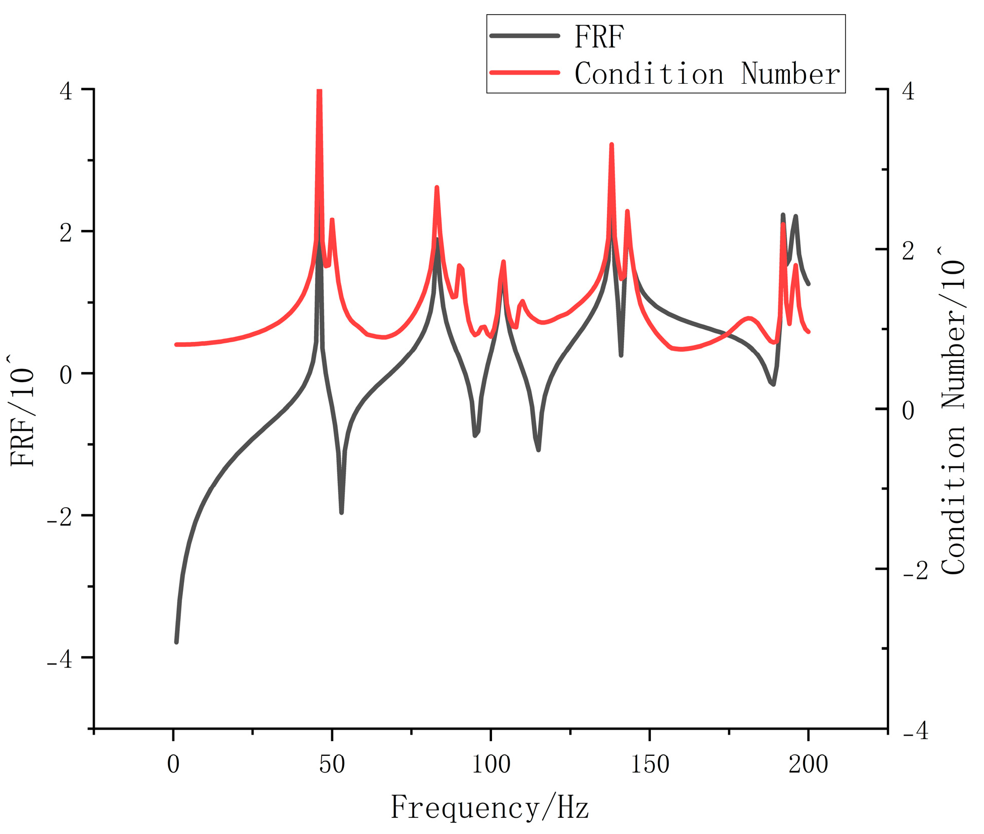
It is set that the amplitudes of the three exciting forces are all 1N, and the excitation is carried out in the full frequency band. The velocity responses of the five structural response points at the corresponding frequencies can be calculated by using the modal superposition formula, and the transfer characteristic matrix is correspondingly obtained. The condition numbers of each matrix and the frequency response function of the simply supported plate are calculated, and the results are compared as shown in Figure 2.

From the above images, it can be found that the condition numbers corresponding to the first four modal frequencies of 46 Hz, 83 Hz, 104 Hz, and 138 Hz are 22,154.1, 600.1, 69.6, and 2049.2, respectively. The condition number curve is highly consistent with the frequency response function curve of the simply supported plate, indicating that there is a correlation between the distribution law of the condition number of the structural transfer characteristic matrix in the frequency band and the modal frequency of this structure. Combining with the definition of the condition number, it shows that near the modal frequency, the structural transfer characteristic matrix has strong ill-conditioning, and the first-order modal frequency has the strongest ill-conditioning.

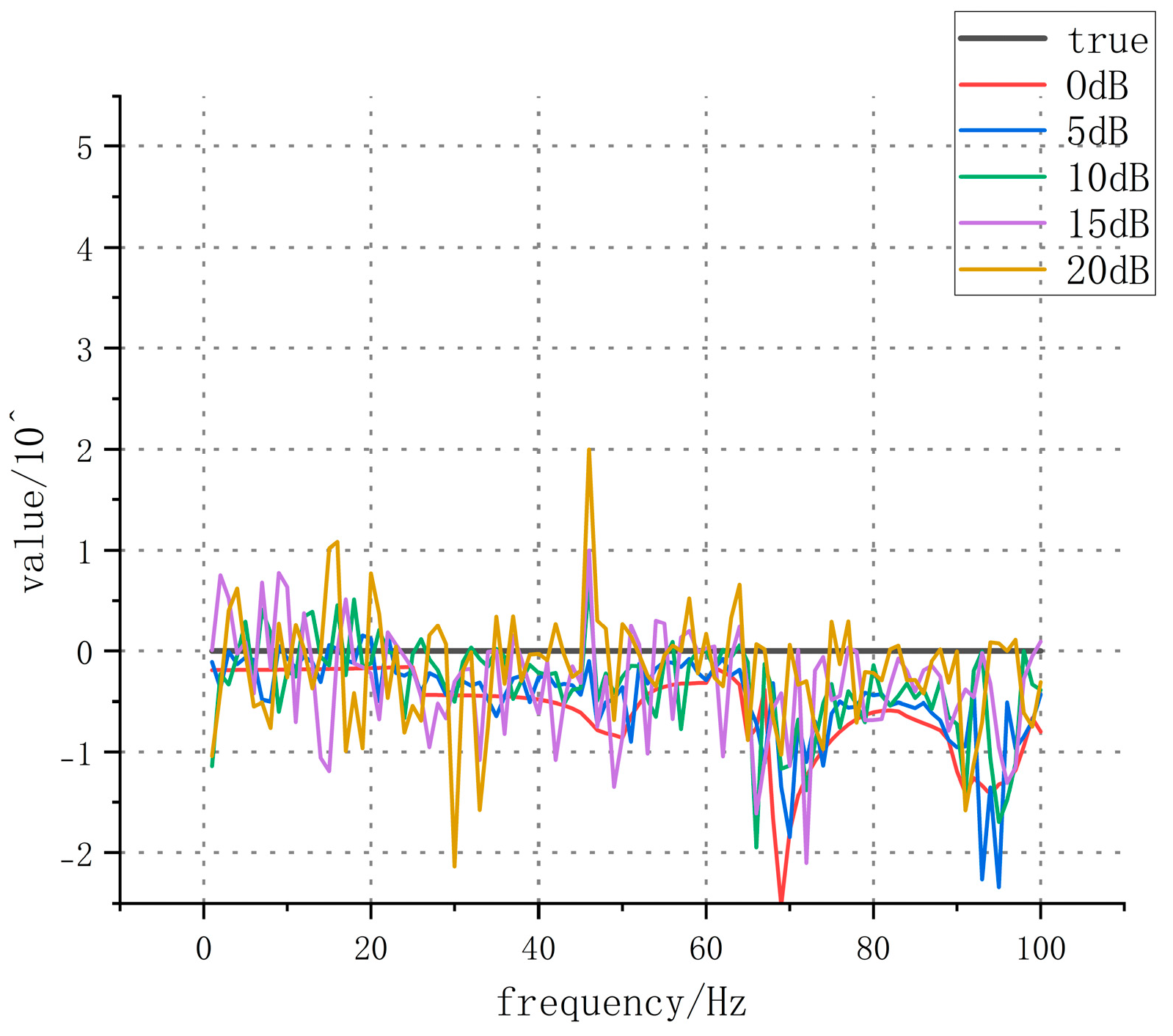
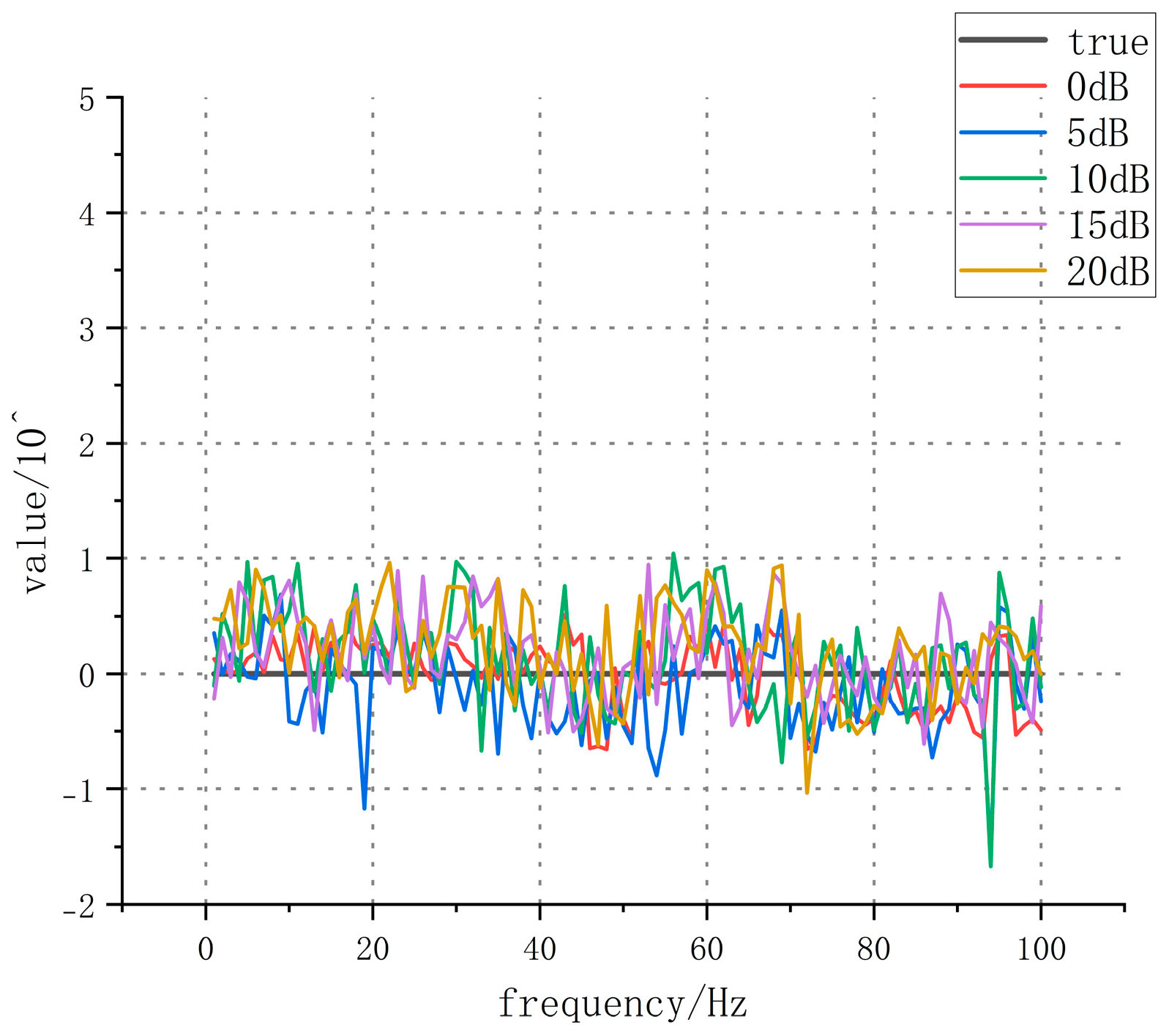
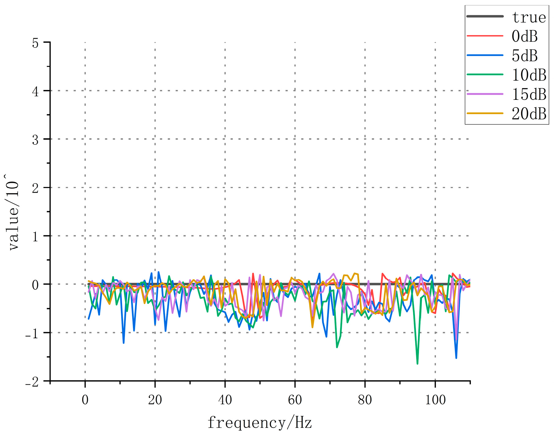
In order to simulate the environmental noise interference in the working environment of the ship, noise interferences of 0 dB, 5 dB, 10 dB, 15 dB, and 20 dB are, respectively, added to the vibration response signals. Then, the ill-conditioned matrices are processed by methods of no correction, TSVD, GCV, L-curve, Q-O and BL-curve, respectively. Subsequently, the magnitudes of the exciting forces are inversely solved, and the results are shown in Figure 3, Figure 4, Figure 5, Figure 6, Figure 7 and Figure 8.

From the results, it can be seen that when the transfer function matrix at the modal frequency (46 Hz) is not processed, even a slight noise interference will lead to a very large error in the inverse calculation of the force. Therefore, it is necessary to correct the ill-conditioned matrix. Meanwhile, the above results demonstrate that traditionally commonly used regularization methods exhibit instability and unsatisfactory outcomes under the interference of background noise. In contrast, the BL-curve and Q-O regularization methods proposed in this paper have achieved the expected results and improved stability in terms of the outcomes.

5. Experimental Validation

To further verify that the improved regularization method can maintain favorable correction performance in practical applications, and to simultaneously test the practical applicability of the real-ship mechanical equipment load identification test procedure proposed in this paper, analytical verification is conducted using test data from a 1:4 scaled cabin section model, respectively.

5.1. Experiment Settings

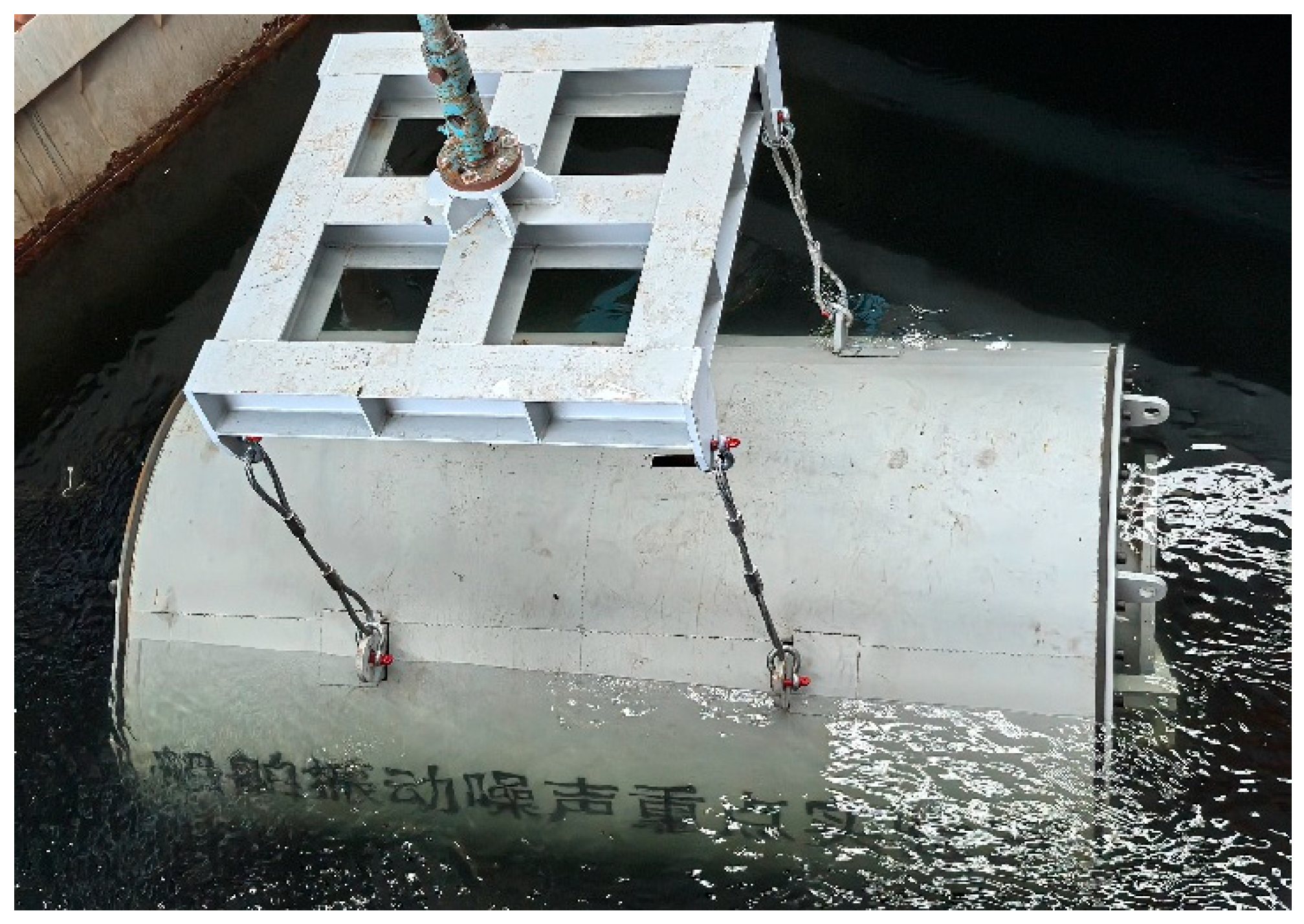
The test model is a 1:4 scaled model of a certain type of ship cabin section. It is structured as a double-shell cylindrical hull with a diameter of 2.2 m and a length of 3.5 m, as shown in Figure 9.

Equipment such as vibrators, seawater pumps, vibration motors, circulating water tanks, and pipeline systems are installed inside the cabin section model. Among them, the ends of the pipelines at the water inlet and outlet of the seawater pump are connected to the outer shell of the scaled cabin section model; all equipment is mounted on small rafts, which are connected to the base via rubber vibration isolators; a large number of acceleration sensors and hydrophones are arranged inside the cabin section. The relevant internal equipment and structure of the scaled cabin section model are shown in Figure 10.

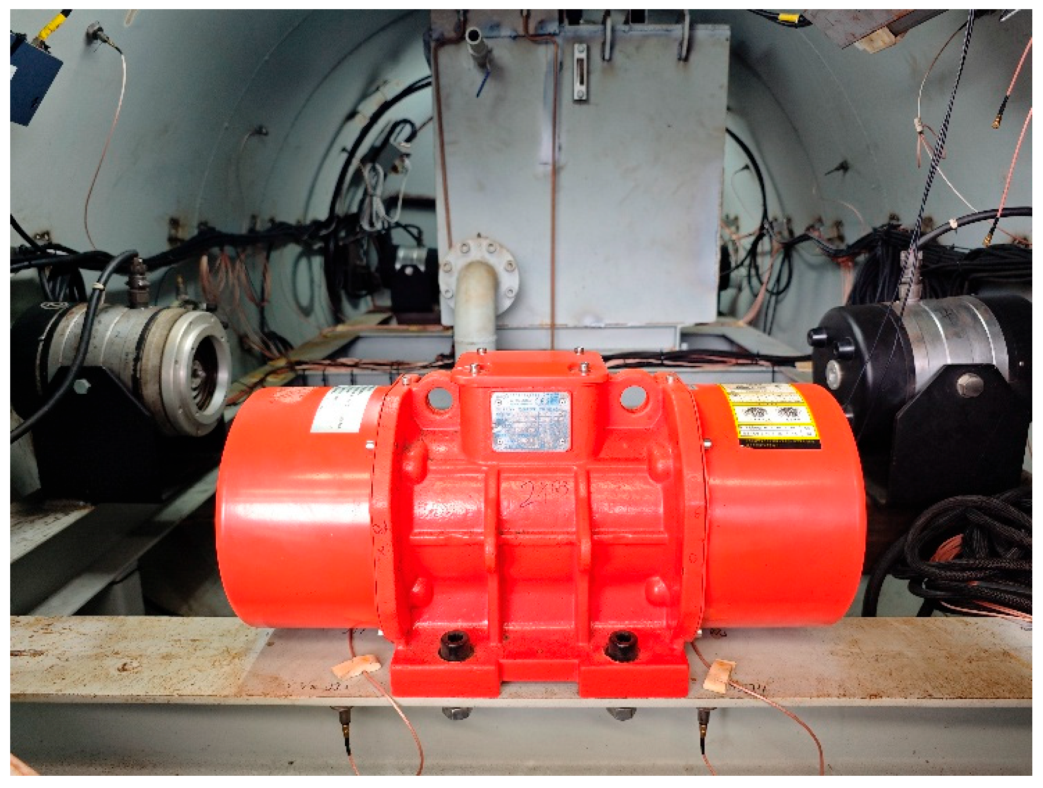
Among them, to better simulate the operation of mechanical equipment on an actual ship, a three-phase vibration motor was selected as the excitation source for load identification and solution, as shown in Figure 11.

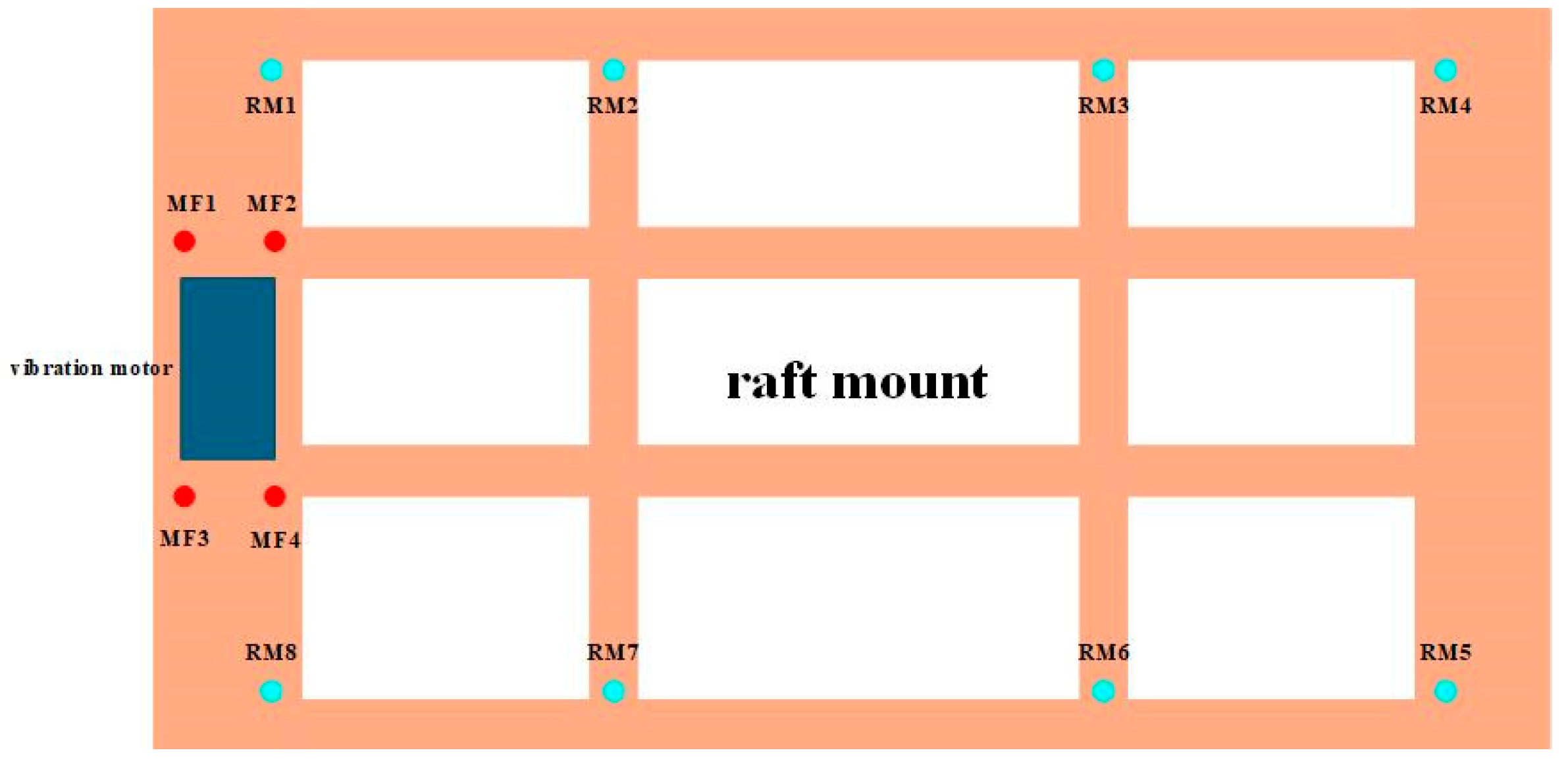
To solve for the excitation force, it is first necessary to determine the positions of the excitation force points and acceleration response points. In this experiment, 4 motor feet near the joint between the vibration motor and the raft mount were selected as the excitation force points, and acceleration sensors were arranged at a total of 8 positions on the raft mount. The specific positions are shown in the following Figure 12.

It should be noted that since the research content of this paper is only related to excitation force inversion, the relevant data and experiments are solely associated with the vibration motor. For this reason, other equipment and sensors at other positions have been simplified in subsequent parts.

Among them, MF1–MF4 represent the excitation force points numbered 1#–4#, respectively, and RM1–RM8 represent the acceleration response points numbered 1#–8#, respectively.

The test acquisition and analysis system mainly consists of data acquisition equipment, acceleration sensors, excitation sources, a force hammer, and a computer. Among them, the acceleration sensors are of the B&K 4513/4514 type; the acquisition equipment is a B&K Pulse acquisition and analysis instrument, which can perform synchronous data acquisition for nearly 100 channels with an analysis frequency of up to 20 kHz; and the force hammer is of the B&K 8207 type.

The testing part mainly includes the following two points.

(a)

Measurement of the acceleration structural transfer function matrix between the exciting force points and the structural response points: By adopting the impact hammer excitation method, MF1-MF4 were excited sequentially, and the response data of RM1-RM8 were measured synchronously. After screening and averaging processing, the transfer characteristic matrix H was calculated.

(b)

Solution and verification of the exciting force: After starting the motor, measure the real response signal ${\mathrm{a}}_{\mathrm{r}\mathrm{u}\mathrm{n}}$ at the structural response points, and calculate the exciting force through the equation ${\mathrm{F}}_{\mathrm{p}\mathrm{s}\mathrm{e}}={\mathrm{H}}^{+}{\mathrm{a}}_{\mathrm{r}\mathrm{u}\mathrm{n}}$. Meanwhile, to verify the accuracy of the excitation force solution and measure the error value, analysis and calculation were conducted through indirect verification. By selecting point RM5 as the verification point for acceleration field reconstruction, the acceleration field during the actual operation of the motor was compared with the reconstructed acceleration field, and the magnitude of the error value was calculated.

5.2. Test Results Analysis

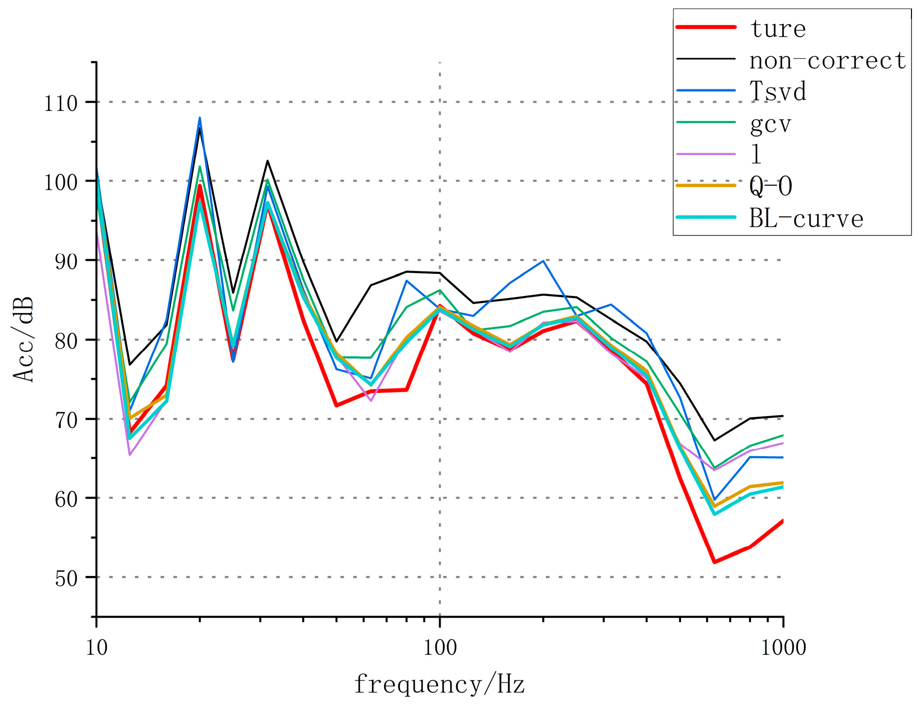
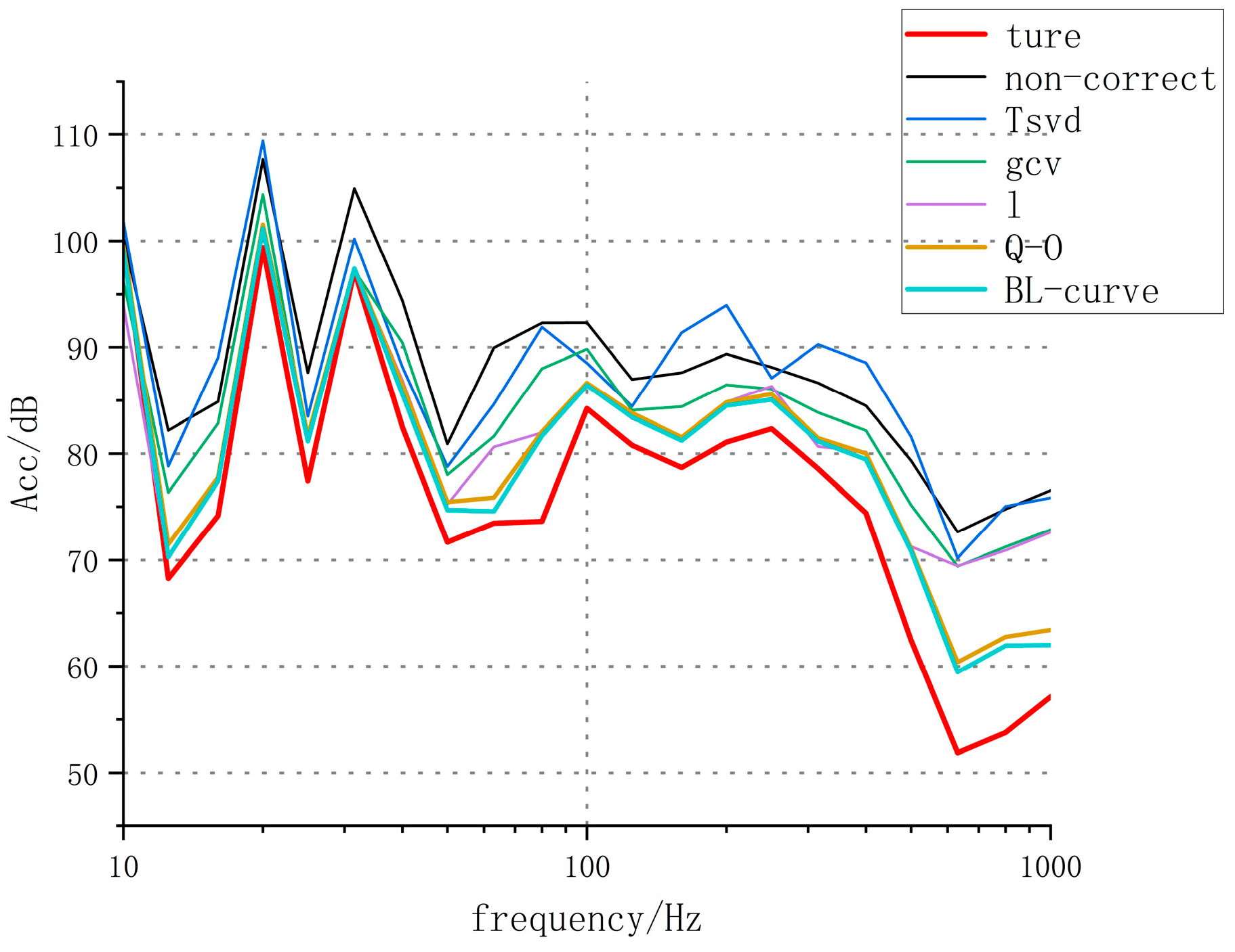
To simulate the complex background noise environment of an actual ship, the author added different levels of noise to the response signals (i.e., the measurement points RM1-RM8) within the frequency band of 10 Hz to 1 kHz and applied different regularization methods for correction. By comparing the acceleration reconstruction error values, the advantages and disadvantages of different regularization methods were evaluated.

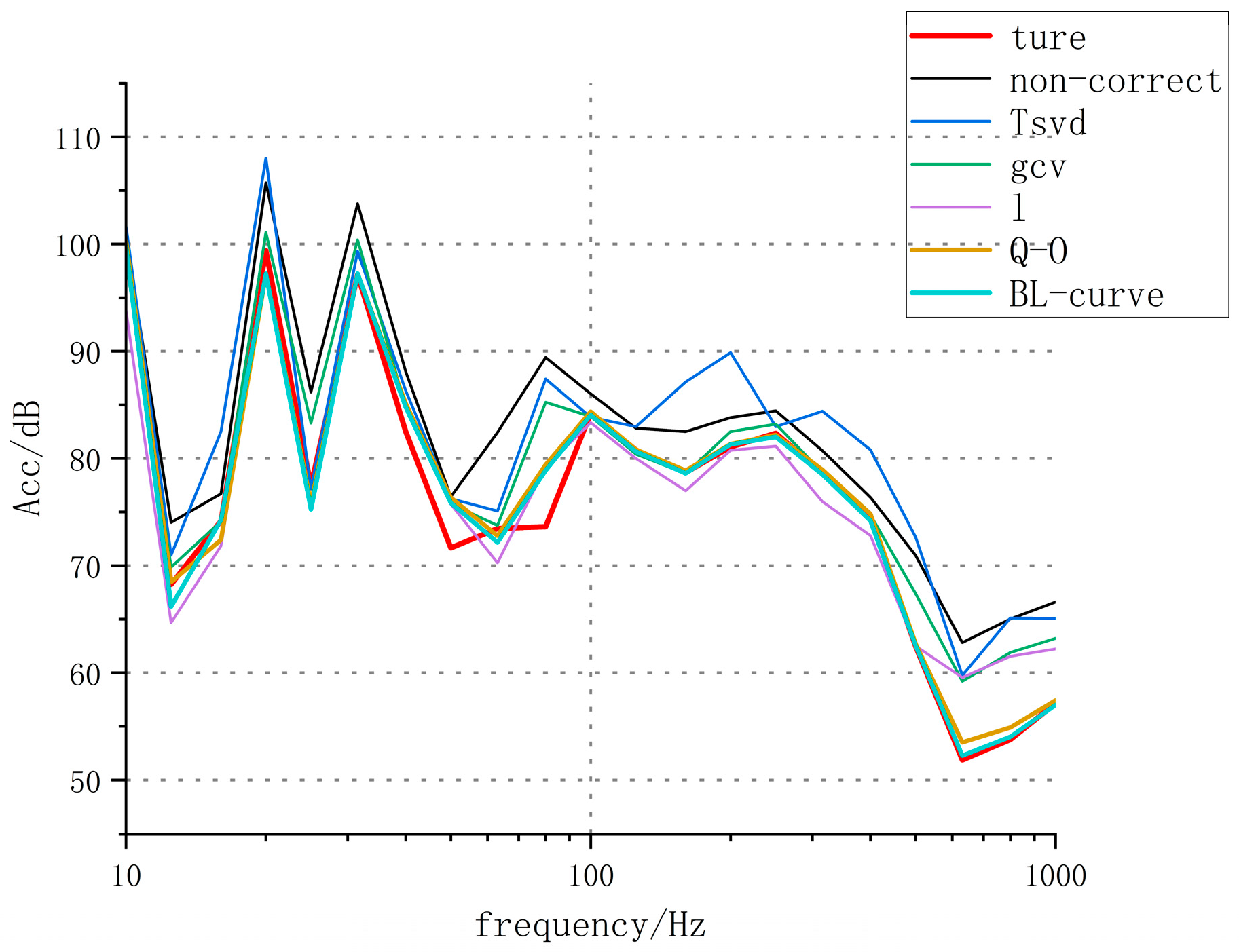
White noise interference of 0 dB, 5 dB, 10 dB, and 15 dB was added to the vibration response signals, respectively. Meanwhile, the truncated singular value decomposition (TSVD), generalized cross-validation (GCV), L-curve, Q-O, and BL-curve regularization methods were employed to calibrate the transfer characteristic matrix H. The 1/3 octave spectral density within this frequency band (10 Hz–1 kHz) was calculated, as shown in Figure 13, Figure 14, Figure 15 and Figure 16. Simultaneously, it was compared with the actual measured values to compute the error.

To more clearly compare the correction effects of different regularization methods, the error values of the 1/3 octave spectrum density within this frequency band were calculated. The calculation formula is:

$$\mathsf{\Delta }={\displaystyle \frac{20}{\mathrm{L}}}{\displaystyle \sum _{\mathrm{i}=1}^{\mathrm{L}}\left|\lg \left({\mathrm{a}}_{\mathrm{i}}/{\widehat{\mathrm{a}}}_{\mathrm{i}}\right)\right|}$$

(23)

where ${\mathrm{a}}_{\mathrm{i}}$ and ${\widehat{\mathrm{a}}}_{\mathrm{i}}$ are the measured and reconstructed values at the i-th center frequency, respectively, and L is the number of octave segments; the 1/3-octave center frequency in the paper is 10~1000 Hz, and L = 21.

The results are shown in

Table 3. Comparison of the error values of the 1/3 octave spectral density after the introduction of different noises.

	1/3-Octave Spectral Density Error
	0 dB	5 dB	10 dB	15 dB
No amendment	4.023	5.836	8.098	11.482
TSVD	4.405	5.607	5.607	10.968
GCV	1.882	2.954	5.041	7.910
L-curve	1.962	2.931	3.507	5.896
Q-O	1.074	1.187	2.551	4.210
BL-curve	0.923	1.036	2.264	3.676

.

From the results, before the transfer characteristic matrix H is corrected, even without the interference of white noise, there is an error of about 4 dB in the error value, which indicates that the ill-conditioning of the matrix has a great impact on the results. Therefore, regularization correction is necessary.

The results of the test data show that in a normal environment, that is, without the interference of noise, the performance of the BL-curve regularization parameter solution method is better than the existing L-curve and GCV methods. Its reconstruction error value is only 0.9 dB, and it is also better than the Q-O method. As the background noise level increases, the calculation error of the radiated noise is smaller than that of methods such as the L-curve. Under high background noise, the cumulative error can be reduced to 3.7 dB, the robustness and stability of the solution are improved, and the evaluation error of the radiated noise is reduced.

At the same time, it can be found that the solution error under the Q-O method is also smaller than that of the L-curve and GCV regularization methods. The reconstruction error value is 4.2 dB under high background noise, and its robustness is better than that of the L-curve and GCV regularization methods.

Therefore, based on the above analysis results, it can be concluded that after optimizing the solution method for regularization parameters, the correction effects of the Q-O and BL-curve regularization methods are relatively significant. They can not only correct the severe ill-conditioning of the matrix at the modal frequencies but also maintain good correction effects under the interference of a large amount of noise. Relatively speaking, the BL-curve method has better robustness.

6. Conclusions

(1)

This paper conducts research on the indirect solution process of excitation forces of marine mechanical equipment. Aiming at the ill-posed problem encountered in the solution of inverse problems, it points out the limitations of traditional regularization methods in application and solution under ships with complex acoustic environments. On this basis, optimized Q-O and BL-curve regularization parameter solution methods are proposed. The feasibility of the methods is verified through simulations and experiments, and the robustness of the regularization methods is improved.

(2)

This paper optimizes the indirect solution method for the excitation force of ship mechanical equipment and verifies it through scaled cabin section experiments. It provides guidance for the subsequent practical application of ships, which can be further implemented in engineering, and helps with ship structural design, acoustic design, radiated noise prediction, etc.

(3)

Meanwhile, further analysis of the experimental results shows that the Q-O regularization method is less effective than the BL-curve method. The reason is that Q-O is improved on the basis of the L-curve. Firstly, it is necessary to roughly estimate the possible value range of the regularization parameter through the L-curve method and then apply the fine-tuning criterion on this basis. However, due to noise interference, the L-curve tends to show local fluctuations. If the initial interval determined by the L-curve method has significant oscillations, the accuracy of the quasi-optimality criterion will also be affected. Therefore, the Q-O regularization method is not perfect and needs to be improved in the future.

References

1. Chen, H.H.; Bao, M. Force identify-cation for mechanical vibration: State-of-the-art and prospect. China Mech. Eng. 2002, 13, 526–531. [Google Scholar]
2. Jiang, J.H.; Zhang, F. Research Progress on Structural Dynamic Load Identification. J. Vib. Eng. 2024, 37, 1625–1650. [Google Scholar]
3. Liu, R.X.; Dobrlban, E.; Hou, Z.C.; Qian, K. Dynamic Load Identification for Mechanical Systems: A Review. Arch. Comput. Methods Eng. 2022, 29, 831–863. [Google Scholar] [CrossRef]
4. Mao, Y.M.; Lin, J.F.; Liu, J.H.; Di, W.B. Recent Advances of Dynamic Force Estimation Techniques. J. Dyn. Control 2014, 12, 97–104. [Google Scholar]
5. Wei, Y.; Xie, P.; Zhang, L. Tikhonov regularization and randomized GSVD. SIAM J. Matrix Analy. Appl. 2016, 37, 649. [Google Scholar] [CrossRef]
6. Chen, Z.; Qin, L.; Zhao, S.; Chan, T.H.; Nguyen, A. Toward efficacy of piecewise polynomial truncated singular value decomposition algorithm in moving force identification. Adv. Struct. Eng. 2019, 22, 2687. [Google Scholar] [CrossRef]
7. Jiang, W.S.; Wang, Z.Y.; Lv, J. A fractional-order accumulative regularization filter for force reconstruction. Mech. Syst. Signal Process 2018, 101, 405. [Google Scholar]
8. Wang, L.; Liu, J.; Lu, Z.R. Bandlimited force identification based on sinc-dictionaries and Tikhonov regularization. J. Sound Vib. 2020, 464, 114988. [Google Scholar] [CrossRef]
9. Choi, H.G.; Thite, A.N.; Thompson, D.J. Comparison of methods for parameter selection in Tikhonov regularization with application to inverse force determination. J. Sound. Vib. 2007, 304, 894–917. [Google Scholar] [CrossRef]
10. Chen, Z.; Chan, T.H.T. A truncated generalized singular value decomposition algorithm for moving force identification with ill-posed problems. J. Sound. Vib. 2017, 401, 297–310. [Google Scholar] [CrossRef]
11. Hansen, P.C. Truncated singular value decomposition solutions to discrete ill-posed problems with ill-determined numerical rank. SIAM J. Sci. Stat. Comput. 1990, 11, 503. [Google Scholar] [CrossRef]
12. Powell, R.E.; Seering, M. Multichannel structural inverse filtering. J. Vib. Acoust. Stress. Reliab. Des. 1984, 106, 22–28. [Google Scholar] [CrossRef]
13. Romano, J.; Lodpez, J.A. Practical application of transfer path analysis to resolve structure-borne noise problems in vehicle design. In Proceedings of the 21st International Seminar on Modal Analysis, Kissimmee, FL, USA, 3–6 February 1996; pp. 527–536. [Google Scholar]
14. Hansen, P.C.; Jensen, T.K.; Rodriguez, G. An adaptive pruning algorithm for the discrete L-curve criterion. J. Comput. Appl. Math. 2007, 198, 483. [Google Scholar] [CrossRef]
15. Qiu, B.B.; Zhang, M.; Li, X.; Qu, X.; Tong, F. Unknown impact force localisation and reconstruction in experimental plate structure using time-series analysis and pattern recognition. Int. J. Mech. Sci. 2020, 166, 105231. [Google Scholar] [CrossRef]
16. Hansen, P.C. The L-curve and its use in the numerical treatment of inverse problems. In Computational Inverse Problems in Electrocardiology; WIT Press: Billerica, MA, USA, 1999; pp. 119–142. [Google Scholar]
17. He, Z.; Zhang, Z.; Li, E. Multi-source random excitation identification for stochastic structures based on matrix perturbation and modified regularization method. Mech. Syst. Signal Process. 2019, 119, 266. [Google Scholar] [CrossRef]
18. He, Z.; Zhang, Z.; Li, E. Random dynamic load identification for stochastic structural-acoustic system using an adaptive regularization parameter and evidence theory. J. Sound Vib. 2020, 471, 115188. [Google Scholar] [CrossRef]
19. Chen, H.; Miao, B.R.; Zhao, L.T.; Zhang, Y.; Jiang, C.Y.; Zhou, F. Research on impact load identification based on L1-norm regularization and least squares optimization. Noise Vib. Control 2023, 43, 62–67. [Google Scholar]
20. Huang, C.; Wang, L.; Fu, M.; Lu, Z.R.; Chen, Y. A novel iterative integration regularization method for ill-posed inverse problems. Eng. Comput. 2020, 37, 1921–1941. [Google Scholar] [CrossRef]
21. Golub, G.H.; Hansen, P.C.; O’Leary, D.P. Tikhonov regularization and total least squares. SIAM J. Matrix Anal. Appl. 1999, 21, 185–194. [Google Scholar] [CrossRef]
22. Fenu, C.; Reichel, L.; Rodriguez, G.; Sadok, H. GCV for Tikhonov regularization by partial SVD. BIT Numer. Math. 2017, 57, 1019–1039. [Google Scholar] [CrossRef]
23. Wang, L.; Peng, Y.; Xie, Y.; Chen, B.; Du, Y. A new iteration regularization method for dynamic load identification of stochastic structures. Mech. Syst. Signal Process. 2021, 156, 107586. [Google Scholar] [CrossRef]
24. Li, X.; Zhao, H.; Chen, Z.; Wang, Q.; Chen, J.; Duan, D. Force identification based on a comprehensive approach combining Taylor formula and acceleration transmissibility. Inverse Probl. Sci. Eng. 2018, 26, 1612. [Google Scholar] [CrossRef]
25. Ruibiao, L.I.; Lin, H.E.; Wenjun, B.U.; Rongwu, X.U. Comparison and experimental study of different regularization methods in ship radiated noise calculation. Vib. Shock. 2021, 40, 151–158. [Google Scholar]
26. Gordon, W.J.; Riesenfeld, R.F. B-spline curves and surfaces. In Computer Aided Geometric Design; Academic Press: Salt Lake City, UT, USA, 1974; pp. 95–126. [Google Scholar]
27. Gunawan, F.E.; Homma, H.; Kanto, Y. Two-step B-splines regularization method for solving an ill-posed problem of impact-force reconstruction. J. Sound Vib. 2006, 297, 200–214. [Google Scholar] [CrossRef]
28. Regińska, T. Two-parameter discrepancy principle for combined projection and Tikhonov regularization of ill-posed problems. J. Inverse III-Posed Probl. 2013, 21, 561–577. [Google Scholar] [CrossRef]
Figure 1. Model diagram of simply supported plate.
Applsci 15 10238 g001
Figure 2. Distribution Curve of the Condition Numbers of the Transfer Characteristic Matrix at Different Frequencies.
Applsci 15 10238 g002
Figure 3. Comparison of the effect of different noises on reconstructed values without correction.
Applsci 15 10238 g003
Figure 4. Comparison of the effects of different noises on the TSVD corrected reconstruction values.
Applsci 15 10238 g004
Figure 5. Comparison of the effects of different noises on the corrected reconstructed values of GCV.
Applsci 15 10238 g005
Figure 6. Comparison of the effect of different noises on the L-curve correction reconstruction value.
Applsci 15 10238 g006
Figure 7. Comparison of the effect of different noises on the reconstructed value of Q-O correction.
Applsci 15 10238 g007
Figure 8. Comparison of the effects of different noises on the corrected reconstructed values of BL curves.
Applsci 15 10238 g008
Figure 9. Actual test scene diagram.
Applsci 15 10238 g009
Figure 10. Model diagram of mechanical equipment.
Applsci 15 10238 g010
Figure 11. Equipment Actual Layout Drawing.
Applsci 15 10238 g011
Figure 12. Measurement Point Layout Schematic.
Applsci 15 10238 g012
Figure 13. 1/3-octave spectrogram of 0 dB background noise.
Applsci 15 10238 g013
Figure 14. 1/3-octave spectrogram of 5 dB background noise.
Applsci 15 10238 g014
Figure 15. 1/3-octave spectrogram of 10 dB background noise.
Applsci 15 10238 g015
Figure 16. 1/3-octave spectrogram of 15 dB background noise.
Applsci 15 10238 g016