Article

A Study on the Soil Seismic Liquefaction Artificial Neural Network Probabilistic Assessment Method Based on Standard Penetration Test Data

1
State Key Laboratory of Simulation and Regulation of Water Cycle in River Basin, China Institute of Water Resources and Hydropower Research, Beijing 100038, China
2
Engineering Research Center on Anti-Earthquake and Emergency Support Techniques of Hydraulic Projects, Ministry of Water Resources, Beijing 100048, China
*
Author to whom correspondence should be addressed.
Appl. Sci. 2025, 15(18), 10229; https://doi.org/10.3390/app151810229
Submission received: 23 July 2025 / Revised: 4 September 2025 / Accepted: 12 September 2025 / Published: 19 September 2025

Abstract

Constructing a probabilistic assessment method is the primary task and key step in liquefaction research. This paper presents a systematic investigation into liquefaction potential evaluation methods. Through a comparative analysis of three conventional assessment methods, we identify critical limitations in existing approaches regarding accuracy and adaptability. A probabilistic ANN model was developed using field-collected standard penetration test (SPT) data from 311 liquefaction case histories. The model demonstrates superior performance with an overall accuracy of 86.17%, achieving 83.33% and 90.00% recognition rates for liquefied and non-liquefied cases, respectively. Key metrics, including precision (91.84%), recall (83.33%), and F1-score (87.38%), indicate robust discriminative capability. Comparative studies confirm the ANN model’s advantages over traditional methods in terms of prediction reliability and operational practicality. The research outcomes offer significant value for improving current liquefaction hazard assessment protocols in geotechnical engineering practice.

1. Introduction

Soil seismic liquefaction refers to the phenomenon where saturated sandy soils or silty sands lose shear strength and stiffness within a short period under dynamic loading, exhibiting behaviors similar to liquid. The essence of liquefaction lies in the instability of the soil skeleton and the rise in pore water pressure. Under liquefaction conditions, surface sand boiling, uplift, subsidence, foundation instability, tilting, and the buoyancy of underground pipelines may occur, posing a serious threat to people’s safety [1]. Therefore, it is essential to study soil seismic liquefaction.
Soil seismic liquefaction research mainly includes three aspects: liquefaction potential evaluation, deformation prediction, and engineering prevention and mitigation [2]. Soil liquefaction likelihood assessment is the foundation of liquefaction research. Currently, various liquefaction assessment methods have been developed, including physical testing, numerical simulation, and empirical equations [3]. Among those, the empirical equation established based on cases is the most commonly used currently and has been incorporated into relevant codes and standards in many countries for guiding engineering practice. Particularly, the standard penetration test (SPT), commonly used in engineering, has accumulated amounts of data under various soil layer depths, soil types, and seismic load intensities, making it widely employed in liquefaction potential assessment [4].
Empirical assessment methods based on SPT data were generally divided into two types: deterministic and probabilistic assessment methods. The deterministic method, represented by the simplified Seed method, provides a binary conclusion of “yes” or “no”, but it cannot provide the specific liquefaction likelihood for a particular case [4]. In the probabilistic method, represented by the R.B. Seed method, featuring an explicit equation, sample parameters were substituted to obtain a specific liquefaction probability [5]. Performance-based seismic engineering design methods are highly recommended currently. Traditional deterministic assessment methods are unable to meet the requirements of superstructure performance design. The methods that can provide specific liquefaction probabilities, even the total liquefaction probability within a future recurrence period, are a hot research topic at present [6].
The current probabilistic statistical methods employed for liquefaction assessment involve statistical modeling grounded on case data, the most common being logical/probabilistic regression and, most recently, machine learning classifiers [7]. As early as 1988, a logistic regression model was proposed for liquefaction probability calculation [8], where parameters such as cyclic shear stress ratio (CSR) and the corrected SPT blow counts ((N1)60) were included. The Bayesian estimation method was employed to consider uncertainties contained in the discrimination result, thereby developing the probabilistic equations for liquefaction assessment [2]. Various liquefaction influence factors were considered and the multiple regression method, First-Order Second-Moment method (FOSM), and joint committee method were employed, respectively for probability assessment, thus promoting the development of liquefaction assessment [9,10,11,12].
Nevertheless, the methods mentioned above were developed based on case datasets from different regions and time periods, with varying amounts of information and representativeness. Additionally, these methods were developed at different times, and the understanding of earthquake-induced liquefaction disasters has evolved over time [5]. Early assessment methods generally assumed that liquefaction would not occur in soils at depths exceeding 20 m and that gravelly soils, due to high permeability and porosity, had low liquefaction likelihood. However, with actual case occurrences in gravel soils and deeply buried sandy soils during the 2008 Wenchuan Earthquake and the 2011 New Zealand Earthquake, methods such as those proposed by Liao and R.B. Seed did not consider the possibilities under gravelly soils, deep burial, and high seismic intensity conditions. Applying these methods directly to these cases inevitably resulted in discriminatory biases [13]. Moreover, the aforementioned methods were built based on the simplified Seed method; the empirical equations typically established include secondary calculated variables like CSR. As a result, a series of assumptions from the Seed method were naturally inherited, and a large amount of uncertainties were introduced, which often lead to relatively conservative assessments. Therefore, it is necessary to adopt appropriate modeling variables to develop new probabilistic assessment methods based on more representative datasets [14].
Another common method for establishing a probabilistic method is combining current machine learning or deep learning approaches. Under the guidance of liquefaction mechanisms and assessment theories, data-driven liquefaction assessment methods were developed [15]. These methods, involving model development, input setup, and a series of mathematical functions, such as logistic functions, were typically used to convert the binary output results into probability values from 0 to 1. The liquefaction potential was then assessed based on the probability value, which aligned with current performance-based liquefaction assessment methods [16].
Accordingly, Muftuoglu and Juang adopted support vector machines and Bayesian networks to study probabilistic liquefaction assessment methods [17,18,19], while Han et al. (2024) and Fan et al. (2025) also integrated different machine learning methods into probabilistic assessment, achieving good classification performance [20,21]. However, the above methods differ in the representativeness of the SPT datasets used, the representativeness of the selected variables, and whether secondary calculated variables were introduced, thereby adding extra assumptions and uncertainties [22]. In machine learning methods, the choice of input data plays a decisive role in determining outcomes. A model has practical significance only when the inputs faithfully represent real conditions. Yet, in current studies, the representative parameter of ground motion—earthquake magnitude—has been inconsistently used, with researchers employing local magnitude (ML), body wave magnitude (mb), surface wave magnitude (MS), or moment magnitude (Mw). Such inconsistencies hinder the model’s ability to reflect actual seismic loading and often cause confusion, since the same earthquake can be assigned different magnitudes, with particularly large discrepancies for small and moderate events. While moment magnitude (Mw) is widely recommended internationally, it tends to perform well only for earthquakes above 7.5, while noticeable biases remain for smaller magnitudes. Therefore, a unified, non-saturating, and globally applicable scale is needed to standardize seismic load input so that it truly captures actual features. To this end, Das et al. have constructively introduced the concept of a generalized moment magnitude (Mwg) and its calculation method. Developed using data from the International Seismological Centre (ISC) and the Global Centroid Moment Tensor (CMT) databases, its formula is given as Mwg = logM0/1.36 − 12.68 [23,24]. Further research is required to train models using this new magnitude scale as an input.
In liquefaction probability assessment, input variables such as seismic loading intensity, soil properties, and site conditions exhibit significant nonlinear relationships and complex interactions. Existing logistic regression methods rely on pre-defined linear or specific functional forms, which are limited in capturing multivariable coupling and high-order nonlinear features. Although support vector machines can introduce nonlinearity via kernel functions, their performance is highly sensitive to kernel type and parameter selection, and their probability outputs require additional calibration [25]. This often results in performance instability under class imbalance or suboptimal parameter settings. Moreover, previous machine learning methods also suffer from limitations such as small dataset size and limited representativeness, dependence on manual feature selection, lack of feature importance analysis, and insufficient applicability under deep burial or high seismic loading conditions. In contrast, artificial neural networks (ANNs) offer multilayer nonlinear mapping and automatic feature combination capabilities, without requiring explicit assumptions about variable relationships. They can simultaneously handle multidimensional, nonlinear, and interaction effects and can directly output threshold-adjustable probabilities, making them more suitable for complex classification tasks like liquefaction probability, which is driven by multiple interacting factors [26].
In recent years, ANNs have been increasingly applied in liquefaction research. For example, Zhao et al. (2022) used a multilayer perceptron model based on standard penetration test (SPT) data to conduct liquefaction classification, achieving overall accuracy superior to logistic regression models, although they did not analyze the model’s generalization capability under different working conditions [26]. Talas proposed a hyper-parameterized ANN architecture, employing random search, grid search, and Bayesian optimization algorithms to predict liquefaction safety factors. While this method achieved higher accuracy than some traditional approaches, it still requires improvement in terms of data diversity, robustness, and interpretability.
The limitations and shortcomings of current liquefaction assessment methods were first reviewed. A soil seismic liquefaction probabilistic model was developed using an artificial neural network based on field liquefaction investigation cases and SPT data. The model’s discrimination results were assessed with five metrics over accuracy (OA), precision (Pre), recall (Rec), F1-score (F1), and area under the ROC curve (AUC). The model’s effectiveness was compared with existing deterministic and probabilistic methods. Further comparative analysis was conducted on the model’s performance across different depth ranges, soil types, and seismic load intensities. Finally, it was applied in a real engineering case from the Ji Ji Earthquake to investigate its applicability. The research results provide a new reference for soil seismic liquefaction probability assessment.

2. Comparative Analysis of Existing Liquefaction Assessment Methods

2.1. Liquefaction Assessment Method Based on Critical Standard Penetration Test Blow Number Criteria

The majority of engineering codes in China rely on critical standard penetration test blow counts as the criterion for liquefaction assessment currently. Liquefaction occurrence was assessed by comparing the field-measured SPT blow counts to the critical thresholds calculated using various established methods [27]. The “Code for Seismic Design of Buildings (GB/T50011-2010)” [20], widely applied in civil engineering; the “Geological Survey Code for Hydropower Engineering (GB50287/2016)” used in hydropower projects [20]; and the “General Principles for Seismic State Design of Building Engineering,” a model standard, were analyzed as examples to highlight the characteristics based on this criterion.
The “Code for Seismic Design of Buildings (GB/T50011-2010)” and “Geological Survey Code for Hydropower Engineering (GB50287/2016)” were constructed based on field liquefaction investigation cases from major earthquakes in the 1960s and 1970s, totaling 156 samples. The data mainly came from the 1970 Tangshan Earthquake. In terms of data characteristics, liquefied sandy layers were mainly distributed at shallow depths, with very few liquefied samples at depths greater than 10 m. The peak acceleration values were mostly within 0.40 g, and no cases were available under higher peak acceleration conditions. When considering seismic intensity and duration time, these are represented by design intensity, seismic grouping, surface peak acceleration, and magnitude, with uncertainties arising from simplified assumptions about seismic loading. The equations and parameters for these two methods were summarized in Table 1.
According to the research of [20], a reasonable critical standard penetration curve should vary rapidly in shallow layers while gradually approaching an asymptote in deeper layers. The ‘General Principles for Seismic Design of Building Engineering’ proposes a new explicit method to overcome the overly conservative nature of the two existing methods when applied to soils at depths of 10–20 m or deeper. The proposed method has been validated under deep-buried sandy soils and strong seismic loading conditions during the Hanshin Earthquake, Ji Ji Earthquake, and New Zealand Earthquake, which expanded its applicability. However, it is a deterministic method and cannot provide specific liquefaction probabilities.

2.2. Liquefaction Assessment Method Based on CSR Criteria

Liquefaction is determined in the cyclic stress ratio method by comparing the cyclic shear stress ratio caused by seismic loading with the soil’s inherent resistance [2]. Based on the cyclic stress ratio theory, various liquefaction assessment methods have been developed and widely applied internationally. The theory was first proposed by Seed et al. and has since been continuously developed and improved, as represented by the NCEER method, the Idriss method, and the Japanese code method [7]. CSR calculation equation forms are consistent, with the specific equation being referenced from Idriss and Boulanger (2006) [9]. Nevertheless, the calculation of specific parameters shows significant differences.
The stress reduction factor, rd, included in the equation was derived from dynamic finite element calculations. Due to differences in the original seismic records, the forms for rd and its values at different depths vary obviously [9]. In particular, for soils at depths below 10 m, the calculated results differ greatly, leading to unreasonable bending of the critical curve under low seismic load conditions. Under strong seismic loading conditions, the critical curve increases with depth, which results in samples with high standard penetration blow counts being determined to be liquefied. The CSR equation involves a series of assumptions and simplifications, introducing certain errors and uncertainties. Additionally, these methods relied on secondary calculated variables, which increased the uncertainty in the discrimination results. Moreover, the mathematical methods used in the development were different, and the datasets they relied on also varied. For instance, the dataset used in the NCEER method only included Seed’s dataset, and the representativeness needs to be further enhanced [2].

2.3. Liquefaction Assessment Method Based on Probability Criteria

Probabilistic liquefaction assessment methods refer to those that can calculate the liquefaction probability of a sample as the final output. Liquefaction is then determined by comparing the probabilities of liquefaction and non-liquefaction. It can be integrated with current performance-based seismic hazard analysis [28]. Probabilistic methods were developed later than the two previous types, beginning around 1988 when Liao et al. established a regression model, and various soil seismic liquefaction probability assessment methods have been developed since then [8]. Explicit methods included the regression model established by Liao et al., the equations established by Kishida and Tsai (2014), and the logistic regression model established by Jas et al. (2024) [15,25]. CSR, as a secondary calculated variable, was used in those methods. Inherited uncertainty from the cyclic stress ratio method was integrated. Sample data for deep burial and high seismic load conditions were still inadequate.
With the rise of machine learning methods, the application in soil liquefaction discrimination has gradually increased, including support vector machine models, neural network models, random forest models, and Bayesian network models. It has no explicit discrimination equations and relies on its own theoretical foundations or introduces logical functions to transform the results into probabilities [14]. Machine learning methods can typically provide liquefaction probabilities, greatly enhancing the practical applicability in soil seismic liquefaction assessment. However, issues still exist. All measured fundamental variables were not integrated during modeling. There was insufficient data representativeness, and there was low discrimination accuracy under deep burial and strong seismic load conditions, and further research is still required [13].
In summary, the liquefaction assessment methods based on critical blow counts, CSR theory, and probability often involve the use of secondary calculated variables instead of original measured variables during modeling. Certain errors or uncertainties were introduced, and the performance declined. Furthermore, data representativeness used in modeling was uneven, and most methods have not been trained on deep burial conditions and strong seismic loading samples, resulting in insufficient assessment ability. Further research is urgently needed for liquefaction probabilistic assessment.

3. Liquefaction Probability Assessment Model Based on Artificial Neural Network

3.1. Collection and Organization of Liquefaction Cases

In this study, for field liquefaction investigation cases, SPT data were systematically collected and integrated, and a dataset comprising nine information items was established. Considering the potential biases inherent in existing magnitude scales, this study adopts the generalized moment magnitude (Mwg) proposed by Das et al [23]—a unified, non-saturating, and globally applicable measure—as the input parameter for earthquake magnitude [23,24]. The magnitudes of the case data are converted into Mwg following the approach described by Das et al. The dataset includes the generalized moment magnitude (Mwg), peak ground acceleration (amax), groundwater table depth (dw), burial depth (ds), total stress (σv), effective overburden stress (σv), fine-particle content (FC), mean grain size (D50), and corrected standard penetration blow counts ((N1)60). The primary data sources include the databases compiled by Cetin et al. (2004) and Idriss and Boulanger (2006), supplemented with additional field liquefaction case histories from the Chi-Chi Earthquake and the New Zealand Earthquake [2,9]. After data compilation, cases with incomplete information were removed, and obvious outliers were cleaned by the box diagram method referenced in the research of Fan et al. (2025), resulting in a final dataset containing 311 data points from 55 earthquakes that occurred between 1944 and 2016, covering major high-intensity seismic zones worldwide [20]. Descriptive statistical analyses were then conducted to examine the distribution of liquefaction cases in the dataset, as summarized in Table 1.
According to the existing research, which suggests that liquefaction generally does not occur when the earthquake moment magnitude is below 5, deep-buried soils still have liquefaction potential [29]. Liquefaction cases have been observed in sandy soils, silty sands, and even gravelly soils. The field liquefaction investigation cases collected in this paper all have earthquake magnitudes above 5, including liquefaction cases in soils below 20 m from New Zealand and Ji Ji. A wide variety of soil types, such as sandy soils, silty soils, and fine sands, was included, and the representativeness of the data was improved [20].

3.2. Analysis of Liquefaction’s Influencing Factors and Determination of Modeling Variables

Referring to the study by Cetin et al. (2018), relying on a single indicator is insufficient to accurately distinguish liquefied and non-liquefied cases [5]. Liquefaction is typically influenced by seismic loading, soil environment, and soil properties [20]. Among those, there is a close relationship between magnitude and the occurrence of soil liquefaction. Larger magnitudes release greater seismic energy, which increases both the intensity and duration of ground shaking, thereby making soil liquefaction more likely. amax is also one of the key indicators for assessing liquefaction potential; higher values indicate stronger seismic shaking and greater dynamic loading on the soil. Intense shaking tends to accelerate the buildup of excess pore water pressure, reduce effective stress, and consequently trigger liquefaction. Therefore, Mwg and amax can be regarded as representative factors of seismic loading.
Groundwater table depth (dw) also plays a significant role in the occurrence of liquefaction. A higher groundwater table increases the saturation of the soil, making pore water pressure more prone to rapid buildup under seismic loading, which reduces effective stress and facilitates liquefaction. Soil burial depth (ds) significantly affects liquefaction susceptibility as well; in general, shallow soils are more vulnerable to liquefaction due to their greater exposure to direct seismic wave action, higher shaking intensity, and slower dissipation of pore water pressure. The total stress (σv) and effective overburden stress (σv) have a significant influence on soil liquefaction. The stress state of the soil affects the contact strength between particles and the stability of the soil structure. Under seismic loading, excess pore water pressure increases, leading to a reduction in effective stress, which in turn decreases the soil strength and may trigger liquefaction. When the total stress and effective overburden stress are relatively high, the liquefaction resistance of the soil is enhanced, and greater overburden pressure helps maintain soil stability and reduce the risk of liquefaction. dw, ds, σv, and σv can therefore be considered representative factors of soil environmental conditions.
The fine-particle content (FC) of soils also has a marked influence on liquefaction potential. As the fine or clay fraction increases, soil permeability decreases, slowing pore water pressure dissipation and increasing the risk of liquefaction. Being a granular material, soil is often characterized in engineering practice by the mean grain size (D50), which reflects particle size distribution and permeability, and is closely related to liquefaction resistance. Soil density is another key factor affecting liquefaction potential: denser soils have more compact particle arrangements, lower void ratios, and greater interparticle contact, resulting in higher shear strength and reduced likelihood of sudden particle rearrangement and pore water pressure buildup under seismic loading. In standard penetration tests, soil density can be approximately represented by the corrected standard penetration blow counts ((N1)60). Consequently, D50, FC, and (N1)60 can be regarded as representative factors reflecting soil properties.
When developing a liquefaction assessment model, it is essential to comprehensively consider representative factors from the perspectives of dynamic loading, soil environmental conditions, and soil properties so as to more accurately capture the mechanism of earthquake-induced soil liquefaction. Mwg and amax can reflect the intensity and duration of seismic motion. ds, dw, σv, and σv can collectively reflect the environmental conditions of the soil during an earthquake. (N1)60, FC, and D50 can serve as the indicators of soil properties and compaction. All the influential factor data were collected in this study, and these nine factors were employed as the base variables for modeling the artificial neural network model in this paper.

3.3. Model Establishment Process and Principles

A feedforward neural network was employed to establish a soil seismic liquefaction assessment model in this paper. The basic theory is to map the input features to the output target space through multiple nonlinear layers of neuronal combinations. The network structure was represented by Equation (1). The form of the artificial neural network is shown in Figure 1.
y = f X ; θ
where Xd represents the input vector, y 2 represents the probabilities of two categories, and θ represents the network weights and biases.
The feature vector that has been normalized using the Min-Max method was received by the input layer, with a dimension of d. The feature combinations in sequence were extracted by hidden layers, and the output calculation of each hidden layer neuron was performed according to Equation (2).
h l = R e   L u W l × h l 1 + b l
where h(0) = X, W(l) ∈nl×l−1, and b(l)nl. The definition of the activation function ReLu was ReLu(z) = max(0,z). Compared with other activation functions, ReLu has a constant gradient within the positive interval, which can significantly accelerate the convergence speed.
The output layer contained two neurons, and the results were mapped as a probability distribution, employing the Softmax method, as shown in Figure 1. Additionally, during the model training process, the training objective was to minimize the cross-entropy loss between the predicted distribution and the true labels [11], as illustrated in Equation (3):
L = 1 N i = 1 N l o g   y i , y i
where yi ∈ {0,1} represents the true sample label, and y i , y i represents the probability.

3.4. Overall Implementation Process of the Model

Traditional liquefaction assessment methods are often based on empirical criteria and statistical regression models. It has certain limitations in terms of applicability. Artificial neural networks, with nonlinear feature mapping ability, excellent adaptability, and generalization capabilities, can model the complex nonlinear relationships between input variables and liquefaction status and can be modeled through multiple layers of neurons [7]. In this paper, a feedforward neural network binary classification model for soil seismic liquefaction assessment was built under the TensorFlow (TensorFlow2.20.0) deep learning framework in a Python environment to achieve precise sample predictions. The calculations for the process in this paper were implemented in PyCharm 2024, and the programming language was Python 3.12.2.
The artificial neural network model training process can be divided into the following stages: data batching, forward propagation, loss function calculation, backpropagation and parameter updates, the early stopping mechanism, etc. Before training data were input into the network, a data splitting method was employed to divide the dataset into several batches. Each batch underwent forward propagation sequentially, where input features XRb×d were linearly transformed by the weight matrices layer and activated by activation functions [7].
In the data batch processing stage, before feeding the raw data into the network, the entire dataset was divided into several smaller mini-batches, with the batch size set to 16 in reference to the study by Zhao et al. (2022) [26]. This batching strategy improves computational efficiency, introduces a degree of randomness into gradient calculations to help avoid local minima, and reduces memory consumption.
The next stage is forward propagation, in which each mini-batch is sequentially passed through the network constructed by the “build_model ()” function. To ensure that the model can effectively capture the nonlinear mechanisms of soil liquefaction, this study conducted multiple rounds of comparative experiments in the preliminary testing phase, varying the number of hidden layers (from two to five) and the number of neurons in each layer (32, 64, 128, 256). The results show that a three-layer fully connected structure achieves a relatively optimal balance between training convergence speed, model stability, and generalization performance. Therefore, the model adopts a sequential architecture comprising three fully connected hidden layers (128, 64, and 32 neurons, respectively), each activated by a ReLU function to introduce nonlinearity, with dropout layers (drop rates of 0.3 and 0.2) inserted after the first two hidden layers to mitigate overfitting. The output layer contains two units with a Softmax activation function to produce the probability distribution for the binary classification task [22].
In the loss function computation stage, the model calculates the prediction error between the output and the true labels according to Equation (3). The loss function “sparse_categorical_crossentropy” is employed during model compilation, which is suitable for multi-class classification problems with integer-encoded labels, and “accuracy” is used as the evaluation metric for real-time monitoring during training [22].
The backpropagation and parameter update stage is automatically executed by the “model.fit()” method, where the backpropagation algorithm computes gradients of the loss with respect to the network parameters, and the Adam optimizer iteratively updates these parameters to minimize the loss [22].
Finally, the early stopping mechanism (“Early Stopping”) monitors the validation loss (“val_loss”). The hyperparameters (learning rate and batch size) were referenced from the method by [22]. Based on the scale of the dataset and available computational resources for this study, multiple pre-experiments were conducted for tuning. The final chosen parameters were a batch size of 16 and an early stopping patience of 20 epochs. Training is terminated if no improvement is observed for 20 consecutive epochs, while “restore_best_weights = True” ensures that the model reverts to the best-performing weights, thereby preventing overfitting. After training, the model uses the “predict()” function to generate probability outputs for the test set, and the predicted class labels are obtained via “np.argmax”. By iteratively executing these five stages, the ANN model gradually converges toward an optimal set of parameters, achieving effective modeling and prediction of the target task. The detailed core source code is provided in the Supplementary Materials.
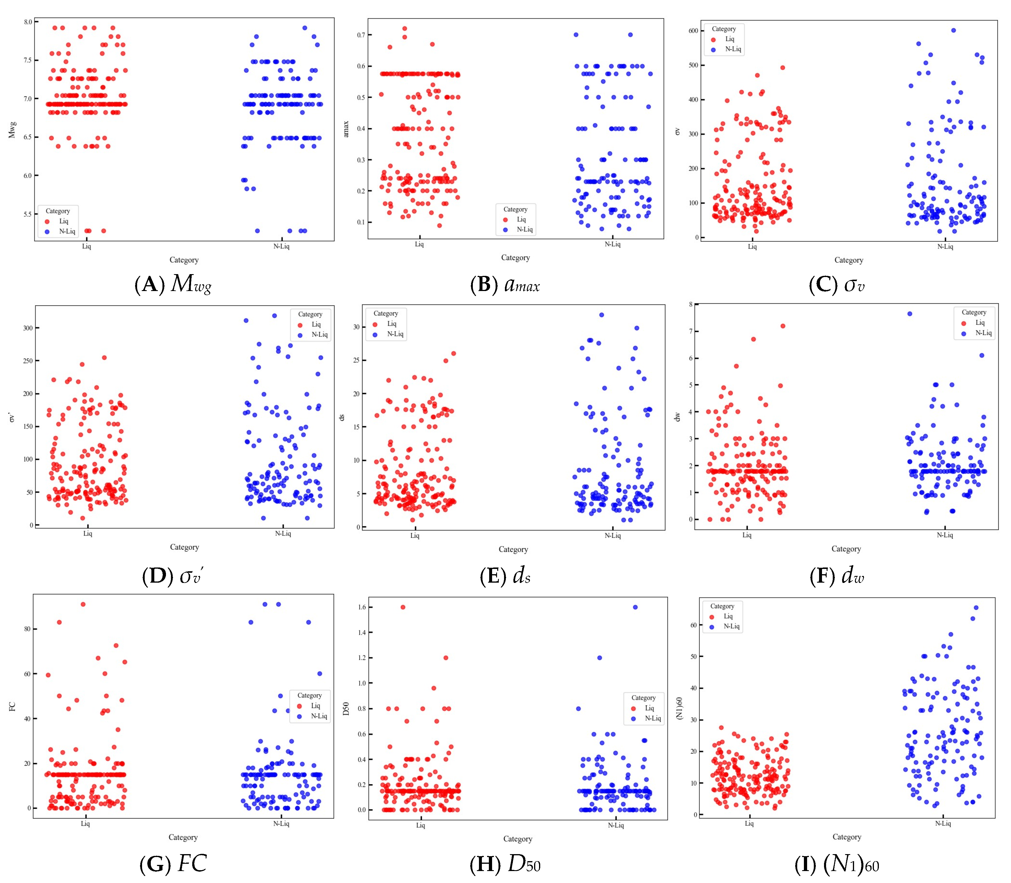
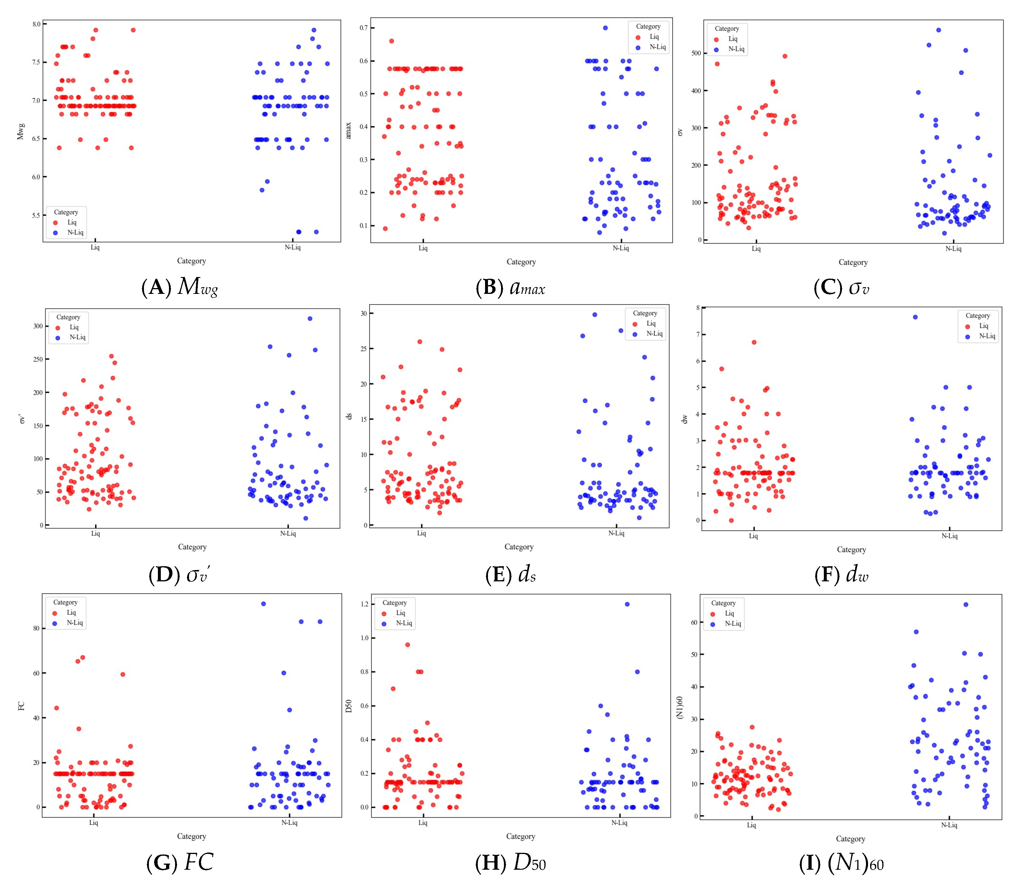
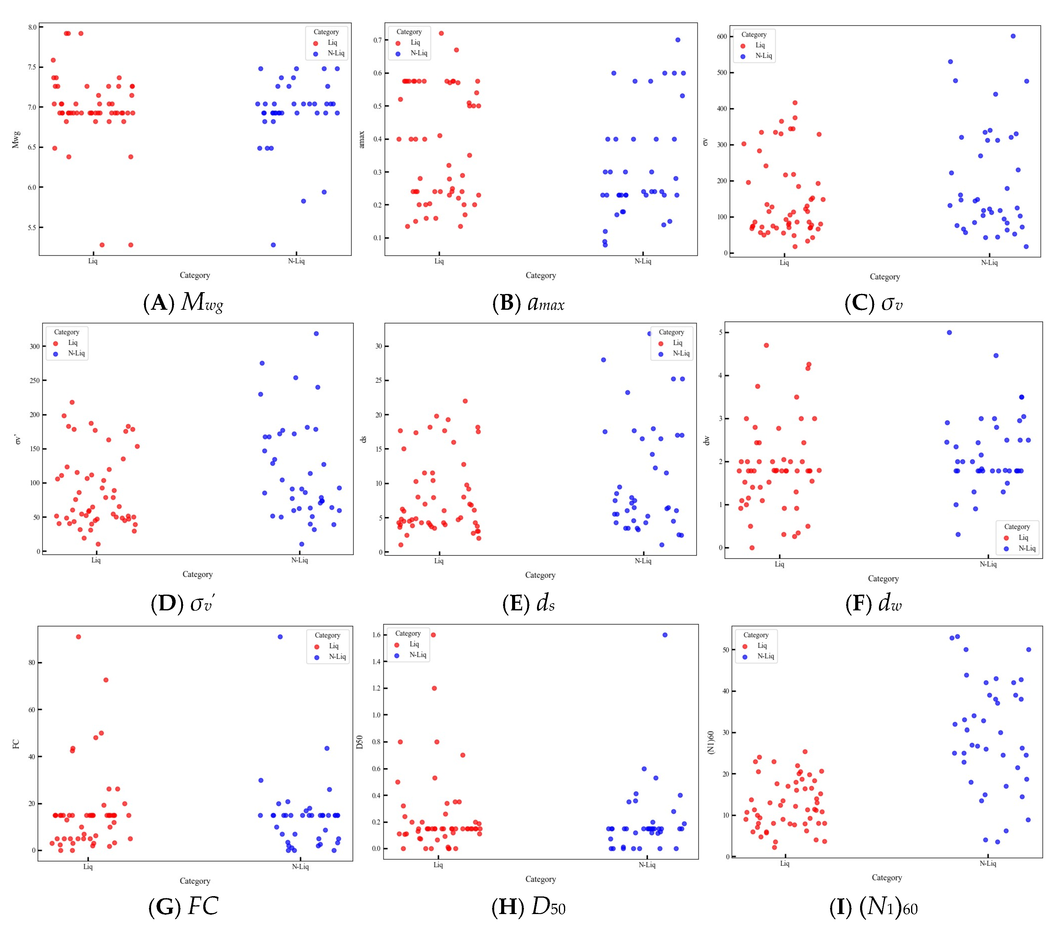
For the specific process of model training, an indicator system was established for the input and output of the artificial neural network model. The complete dataset was normalized using the MinMaxScaler, scaling all input features to the range [0,1]. The data were then randomly split into 70% training and 30% testing subsets with stratification (random_state = 42), ensuring that class proportions remained consistent across both sets. During training, 20% of the training set (approximately 14% of the total dataset) was further set aside as a validation set, which was used to monitor the validation loss (val_loss) and enable EarlyStopping. Consequently, the final data allocation was approximately 56% for training, 14% for validation, and 30% for testing. The data distribution of different variables in each dataset is shown in Figure 2, Figure 3, Figure 4 and Figure 5. It should be emphasized that the test set was not involved at any stage of training or tuning and was only used for the final model evaluation.
The loss and accuracy on both the training and validation sets for each epoch were calculated during the training process. The validation set loss was monitored by the early stopping mechanism. If it did not decrease over 20 consecutive epochs, training was automatically stopped, and the weights corresponding to the best validation set performance were restored. It can effectively prevent overfitting on the training set, and the model’s generalization ability on unseen data was improved. Once training was completed, weight parameters, loss curves for both training and validation, and classification performance metrics were output [22].
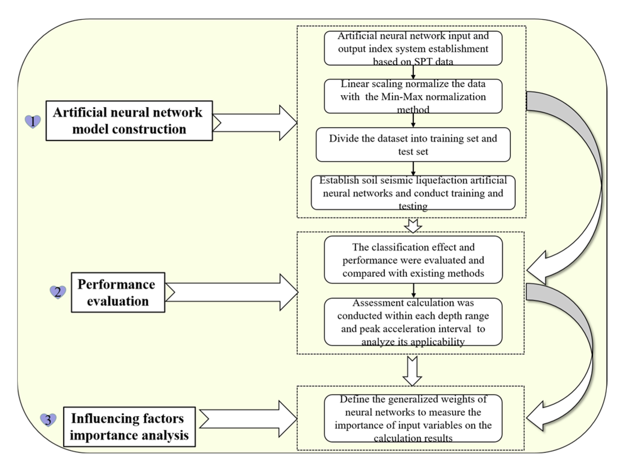
Afterward, a neural network was constructed under the TensorFlow Keras framework, featuring a deep feedforward neural network with three fully connected hidden layers. The input layer was based on the indicator system constructed from SPT data, and the output was a binary classification. In the hidden layers, the ReLU nonlinear activation function was employed for each neuron, while the Softmax activation function was applied for the output layer [22]. Sparse categorical cross-entropy was then used as the loss function, and the Adam adaptive optimizer was employed for gradient descent iterations. The model’s maximum training cycles were set, and early stopping monitors the validation set loss to complete model training. The liquefaction probability for each sample was output on the test set after training. Finally, the importance of each input variable on the calculated liquefaction probability was analyzed. The overall model implementation flowchart is shown in Figure 6.

3.5. Calculation of Model Performance Evaluation Indicators

It is necessary to evaluate model performance after the model has been trained completely. Soil seismic liquefaction assessment is essentially a classification problem. For classification models, the confusion matrix provides an intuitive way to describe the classifier’s ability to assign actual samples to different categories. It compares the predicted results of the classifier with the true classes by calculating the counts of true positives (TP), false positives (FP), true negatives (TN), and false negatives (FN) [13]. Based on the confusion matrix, several evaluation metrics can be computed.
Table 2 presents the equations for these metrics and the corresponding model performance they can reflect. A comprehensive assessment of the model’s performance can be conducted with the confusion matrix and related metrics, which help to identify its strengths and weaknesses. These metrics provide a way to visualize and quantify model results, facilitating comparison, selection, and optimization.

4. Research Results

4.1. Evaluation of the Model’s Discrimination Performance on Test Set Samples

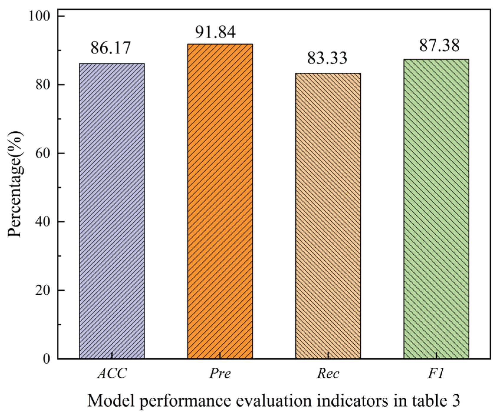
After training and testing the model using the artificial neural network model implementation process shown in Figure 1, the model performance evaluation metrics were employed to assess the discrimination effect. The results are illustrated in Figure 7.
As indicated in Figure 7, the ACC of the model on the test set is 86.17%, which was quite high, indicating the good ability in classifying cases. The Pre, Rec, and F1 scores of the model were 91.84%, 83.33%, and 87.38%, respectively, demonstrating it has high precision and recall rates. Moreover, the F1 score, as the harmonic average of precision and recall, is also at a high level, indicating that the model had excellent classification prediction performance and can efficiently determine whether liquefaction occurs in the soil.
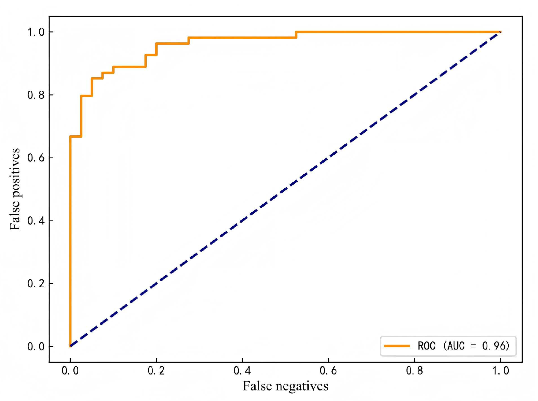
The model’s receiver operating characteristic (ROC) curve calculation results are illustrated in Figure 8. It is commonly employed to assess a classification model’s performance by describing it at different thresholds. The curve reflects the model’s training performance, with the area under the curve (AUC) serving as an indicator of the model training process quality. A higher AUC indicates better model performance. The AUC of the artificial neural network model proposed in this paper was 0.96, indicating that a model with strong classification ability can successfully discriminate seismic liquefaction cases based on probabilistic significance.
To further clarify the model’s applicability under different soil types, depth ranges, and seismic load intensities, the model’s reliability and generalization ability were validated. The test set samples were classified according to the research of Fan et al. (2025) [20], with the ds divided into three categories: 0–10 m, 10–20 m, and greater than 20 m. amax was categorized according to Hu et al.’s method [13] and divided into four levels: 0.07–0.13 g, 0.13–0.24 g, 0.24–0.44 g, and 0.44–0.83 g, corresponding to moderate, strong, very strong, and intense seismic intensities, respectively. Soil properties were classified based on Fan et al. (2025) into four categories: loose, slightly dense, moderately dense, and dense, with corresponding (N1)60 values of (N1)60 ≤ 10, 10 < (N1)60 ≤ 15, 15 < (N1)60 ≤ 30, and (N1)60 > 30 [20]. The discrimination performance of the artificial neural network model proposed in this paper under each condition was analyzed, and the calculation results were summarized in Table 3. In the Table 3, “/” indicates that there are no samples in this interval of the test set. Liq and N-Liq represented the liquefaction cases and non-liquefaction cases, respectively.
As illustrated in Table 3, the model showed good discrimination accuracy across samples under different depth ranges, peak acceleration conditions, and soil property conditions. At the depth of 0–10 m, the accuracy for liquefaction and non-liquefaction cases was 76.32% and 84.00%, respectively, indicating a good classification performance. At depths below 10 m, the model successfully discriminated all liquefaction and non-liquefaction cases, demonstrating remarkable ability under deep burial conditions. It compensated for the limitation of existing methods that are mostly only applicable within 20 m depth and extended the applicability of current methods.
Except for the samples within the range of 0.13–0.24 g, the model’s liquefaction discrimination results were somewhat conservative; the model performed excellently in other peak acceleration ranges. It was convenient for liquefaction assessment under moderate seismic loading conditions and can also successfully classify under intense seismic load intensities. The performance limitations of existing methods under strong seismic loading were improved. Further analysis of the samples that were not successfully classified in the 0.13–0.24 g peak acceleration range revealed that the liquefaction probability was between 30% and 50%. According to the research by R.B. Seed et al. [2], these samples may be close to the critical curve, and the model failed to fully classify liquefaction samples near the critical curve but successfully classified almost all non-liquefaction samples, indicating that the model was slightly conservative. Its performance on critical samples can be improved in the future by adjusting the hyperparameters of the neural network. Additionally, the model showed good discrimination performance with different compaction levels and demonstrated a certain degree of balance, making it applicable to liquefaction assessment under various soil conditions.
Table 4 presents the misclassified cases of the model. When considering individual factors, the potential for misclassification exists within different intervals of each variable, indicating that relying solely on one factor is insufficient for accurate classification. However, when analyzing from the perspective of seismic load, it is evident that misclassified samples generally have a magnitude lower than 7.5, with amax at relatively low levels. This suggests that the model is conservative in classifying samples with low seismic intensity, while almost all samples with strong seismic loads are correctly identified. Future improvements can be made by optimizing model parameters to enhance classification accuracy for such samples.

4.2. Comparison of the Model with Previous Methods

Liquefaction assessment results of the artificial neural network model for the test set samples were presented in Section 4.1, and the model’s generalization ability under different depth ranges, peak accelerations, and soil property conditions was analyzed. Based on this, a comparative analysis was conducted between the model and existing deterministic and probabilistic liquefaction methods. The comparison methods employed were drawn from currently promoted methods both domestically and internationally, as well as the latest research. Deterministic methods include the NCEER method [3], the Idriss method [9], the Geological Survey Code for Hydropower Engineering of China (denoted as the Code method) [20], and the General Principles method (also known as the principle method) [30]. Probabilistic methods include the logistic regression model (LRM) [8] and the support vector machine (SVM) model [13]. The principles, calculation processes, and meanings of equations for each method were referenced from Fan et al. (2025) [20]. Specifically, the discrimination equation of the NCEER method is as shown in Equations (4)–(6). The liquefaction discrimination equation of the Idriss method are as shown in Equations (4)–(7). The calculation equation of the Code method is as shown in Equations (8) and (9). The discrimination equation of the Principle method is as shown in Equations (9) and (10), and the probability calculation equation of the LRM method is as shown in Equation (11). The calculation equation of the R.B. Seed method is shown in Equation (12). The discrimination and establishment process of the SVM model can be found in the previous research of the author of this article, Fan et al. (2025) [20].
C S R C R R
C S R = 0.65 a m a x g σ v σ v r d
C R R = 1 34 N 1 60 + N 1 60 135 + 50 10 N 1 60 + 45 2 1 200
C R R = e x p N 1 60 14.1 + N 1 60 126 2 N 1 60 23.6 3 + N 1 60 25.4 4 2.8
N c r = N 0 β [ I n 0.6 d s + 1.5 0.1 d w ] 3 / ρ c
N N c r
N c r = β 69 a max a max + 0.4 1 0.02 d w 0.21 + 0.79 d s d s + 6.2 3 / ρ c
P L = 1 1 + F S 1.06 3.8
P L = Φ N 1 60 1 + 0.004 F C 13.32 L n C S R 29.53 L n M w 3.7 L n σ v P a + 0.05 F C + 16.85 2.7
where N0 is the standard penetration test blow number benchmark value, β is the adjustment coefficient, amax is the peak acceleration, ds is the depth, dw is the groundwater table, ρc is the clay particle content, Ncr is the critical SPT blow counts, FS is the safety factor, PL is the liquefaction probability, Φ is the normal function, and Pa is the atmospheric pressure.
Comparison as well as the calculation results of the model evaluation metrics were illustrated in Table 5. The artificial neural network (ANN) model proposed in this paper has the highest ACC among all methods, reaching 86.17%. The ANN outperforms other models in Pre, achieving 91.84%, while its Rec is at a moderate level. Accuracy and recall measure different aspects. Precision refers to the proportion of correct predictions among all predictions, while recall focuses on whether the model can correctly identify all actual positive samples. For the evaluation of soil seismic liquefaction, an accuracy of 91.84% indicates that 91.84% of the cases predicted by the model as liquefied are actually liquefied, which shows that the model has high accuracy in identifying liquefaction cases. Although the recall rate is moderate, meaning the model may miss some liquefaction cases (i.e., false negatives), this conservative approach is acceptable in practical engineering applications as it provides a certain safety margin, avoiding the risk of missing liquefaction cases. Given the class imbalance in the dataset, the ANN tends to predict the majority class (non-liquefied cases), and even though it misses some liquefaction cases, it is still able to maintain high accuracy. Therefore, the ANN model is recommended for soil seismic liquefaction probabilistic assessment.
Further analysis of the case data revealed that the dataset used in this study has a liquefaction-to-non-liquefaction case ratio of 178:133, indicating some degree of class imbalance in both categories. For soil seismic liquefaction evaluation, the number of liquefaction cases is higher than that of non-liquefaction cases, and the model may tend to predict liquefaction in order to achieve higher accuracy. Therefore, class imbalance is indeed a significant factor contributing to the moderate recall rate of the ANN. It represents a limitation of the current model, and in the future, sampling techniques could be introduced to balance the class distribution, leading to a more balanced performance.
In terms of model computational efficiency, the ANN model typically requires longer training times and more computational resources [13]. Its training process involves extensive parameter updates, necessitating high memory and processing power, especially when the dataset is large. As a result, the training process may be more resource-intensive compared to other methods. In this study, although the training of the ANN model requires more computational resources, the computational cost is deemed acceptable considering the model’s accuracy and performance. To further enhance efficiency in practical applications, hardware acceleration (such as a GPU) or model optimization techniques (such as pruning, quantization, etc.) can be used in the future to reduce the computational burden.
Figure 9 presents the confusion matrix of the ANN model’s predictions for the two classes of samples. In the dataset, 83.33% of liquefaction cases were accurately predicted by the ANN model as liquefied; 16.67% of non-liquefaction cases were misclassified as liquefied, resulting in false positives; 10.00% of liquefaction cases were misclassified as non-liquefied, resulting in false negatives; and 90.00% of non-liquefaction cases were correctly predicted as non-liquefied. This shows that the model performs well in recognizing both liquefaction and non-liquefaction samples, especially in correctly identifying non-liquefaction samples, where the accuracy is high (90%). Although the model performs excellently, there is a certain false positive rate, indicating that the model mistakenly predicts some non-liquefaction samples as liquefied, showing a slight conservatism. In the future, sampling techniques or further optimization of the model can be applied to improve overall performance, especially in reducing false positives and false negatives.
The accuracy for all samples, as well as samples under different depth conditions, was presented in Table 6. For samples beyond the applicable depth range of the method, the upper equation was continued to apply for calculation. The overall accuracy of the ANN model was the highest among all methods, and its balance between liquefaction and non-liquefaction cases was also higher than that of others. For samples within the 0–20 m depth range, the overall accuracy of the ANN model was 85.23%, the highest among all methods. The accuracies for liquefaction and non-liquefaction cases were 83.32% and 88.57%, respectively. Some liquefaction cases were occasionally classified as liquefied, indicating some conservatism. Future study on prediction accuracy can be conducted by adjusting the neural network’s hyperparameters.
For depths below 20 m, the model successfully classified all samples, with the same discrimination results as the SVM model and outperforming other methods. The applicability of current methods was extended. Additionally, the specific prediction results and liquefaction probabilities for each sample were summarized in Table 7. It is clearly evident that the model’s predicted probabilities for liquefaction and non-liquefaction cases rarely approach the 50% probability level, which indicates that it is highly confident in its predictions. The model demonstrated favorable performance.
One significant advantage of the ANN model is its efficiency in performing liquefaction classification during both operation and inference once the appropriate number of hidden layers and neurons has been determined. Therefore, in the future, if massive datasets are collected in the field of soil seismic liquefaction classification, the model has the potential to process real-time data streams. A survey of current industry applications using artificial neural networks (ANN) for real-time evaluation and large-scale computations reveals that ANN is feasible for both of these application scenarios, but its actual performance may depend on various factors [13]. Firstly, the feasibility of real-time evaluation depends on the model’s inference speed and computational resources. In this case, using GPU acceleration or cloud computing platforms can improve inference speed, ensuring the model meets real-time evaluation requirements. For large-scale geotechnical surveys or liquefaction assessments using the ANN model, it also shows potential. Geological data often involve large sample sizes and complex patterns. Through parallel and distributed computing, the ANN model can efficiently handle massive data, ensuring the timeliness and accuracy of predictions. Similarly, processing large-scale data comes with significant computational costs, so in these applications, future improvements could include the adoption of incremental or online learning methods. This would allow the model to gradually adapt to new data, avoiding the computational bottleneck of retraining the entire model [26].

4.3. Liquefaction Influence Factor Analysis

In addition to an accurate prediction result, another advantage of the artificial neural network model compared to other methods is that it can assess the impact of various factors on liquefaction by evaluating the weight distribution of the neural network model. Generally, the greater the weight assigned to a variable, the greater influence on the model, and the more sensitive the model output is to that input feature [27]. The factors of seismic load (Mw, amax), soil environment (ds, dw, σv, σv), and soil properties ((N1)60, FC, D50) were considered when constructing the artificial neural network. The importance coefficient of each factor’s impact on liquefaction probability, wi, can be calculated with Equation (13):
w i = j = 1 n v i × w i j i = 1 m w i j
where i = 1, 2,…, m, j = 1, 2, …, n, m, n represents the number of neurons in the input layer and hidden layer of the neural network, respectively; vi represents the connection weights of the hidden layer; and wij represents the comprehensive weight of the input layer and the hidden layer.
The sunrise chart of the impact for each variable on the liquefaction assessment results is illustrated in Table 8. The influence of seismic load, soil properties, and soil environment was increased in order of the assessment results, with respective percentages of 28.21%, 46.88%, and 41.40%. Soil environment conditions were the most important factor. It is understandable that those environmental conditions include the groundwater table, depth, and the stress state of the soil. If the groundwater table is located below the measured soil layer or at a deeper level, and the soil at the measurement point is unsaturated or extremely dry, liquefaction will not occur even under intense seismic loading conditions.
In terms of the specific contribution of influencing factors, (N1)60 and amax have the greatest impact on the calculation results, with influence levels of 20.28% and 14.37%, respectively. (N1)60 reflects the soil’s compaction level, which obviously affects the soil’s plasticity and drainage capacity, thereby having a marked impact on liquefaction. amax, on the other hand, reflects the strength of the soil’s response under seismic loading, and the intensity of seismic load is the fundamental cause of liquefaction; the influence on liquefaction is also evident. The conclusion drawn in this paper is consistent with existing research [9].

4.4. Engineering Application

The field liquefaction investigation case of the SPT borehole Yuanlin-YL-BH-6 was selected as the research object. Seven previous methods and the ANN model mentioned in this paper were employed to evaluate the typical site liquefaction and analyze the performance of each method, clarifying the reliability of the proposed ANN model for practical engineering applications. The actual engineering case in this study came from the 1999 Earthquake, during which widespread sand soil liquefaction occurred in Taiwan, China. A large number of field standard penetration tests were conducted, and the data were sourced from the research of [19].
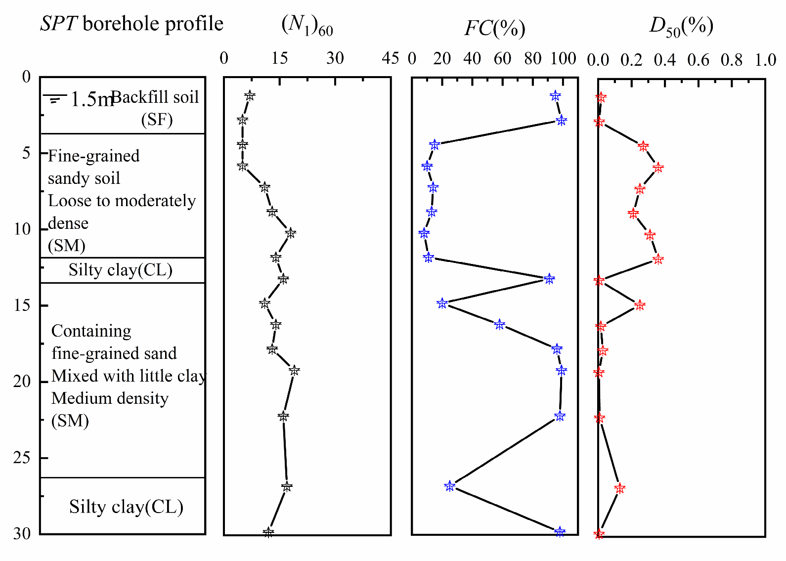
The 1999 Ji Ji Earthquake had a magnitude of Mw = 7.6. The Yuanlin-YL-BH-6 borehole was located near Yuanlin Township in Zhanghua County, Taiwan. During this earthquake, severe liquefaction of sandy soils occurred in the town, resulting in liquefaction-related disasters. The borehole was located at a longitude of 120.56° and a latitude of 23.97°. The maximum surface peak acceleration measured was 0.19 g, and the groundwater table was 1.5 m. The borehole profile is shown in Figure 10. The soil layers consisted of fine sand and silt layers, and it was in a saturated state. Preliminary assessment using the Code method indicated that it is possible for liquefaction under strong seismic loading, and further assessment is required. The assessment results from various methods were shown in Figure 10.
Typical site liquefaction assessment results for each method are illustrated in Figure 11. There were significant differences in the calculation results. For the Yuanlin-YL-BH-6 borehole, the NCEER, Idriss, and LRM methods concluded that liquefaction occurred in the soil within 1.5 m below the surface, while other methods, including the ANN model, suggest that the soil at this depth did not liquefy under the seismic conditions. The soil within 1.5 m was in an unsaturated state, with almost zero likelihood of liquefaction. The results from the three methods above appear slightly conservative under these conditions.
The Idriss method, R.B. Seed method, LRM method, and Code method all indicated that liquefaction would occur in the third layer of the silty clay layer. However, according to the field survey results, no significant liquefaction was observed at the borehole site. It demonstrated that the calculations of these methods were somewhat conservative. The R.B. Seed method and Code method classified soils below 20 m as liquefied, which does not align with the actual observations, indicating that the application under deep burial conditions required further improvement. The ANN model proposed in this paper considered the 1.5–4.5 m soil layer as liquefied, which was inconsistent with the actual observations and slightly conservative. It was consistent with the conclusions drawn from the above liquefaction assessment process and can be improved further to enhance its classification accuracy. Overall, the model proposed in this paper classified significantly fewer soil layers as liquefied compared to others, demonstrating a lower degree of conservatism, making it a recommended probabilistic assessment method.
It is worth noting that the dataset used in this study was collected from around the world, covering most of the major high-intensity seismic zones globally, as well as samples with different burial depths and soil types. The model training and validation processes have proven effective under these conditions. Although the proposed model in this study was only analyzed using actual engineering cases from the Chi-Chi Earthquake, the ANN model proposed here can be applied to liquefaction evaluation in different seismic zones worldwide. However, in the future, as the dataset is further updated, cases from different regions across the globe should be used for more comprehensive validation to demonstrate the model’s generalization capability. In addition, the dataset contains liquefaction samples from different time periods, which may introduce potential biases and uncertainties—for example, differences in experimental errors and measurement standards across regions. These factors were not considered in the model training process of this study, and future work should further analyze the impact of such potential uncertainties on model performance.

5. Conclusions

Three types of liquefaction assessment methods based on critical standard penetration blow counts, CSR theory, and probability were qualitatively analyzed in this paper; the limitations and shortcomings of existing methods in practical applications were also explored. Based on the established field liquefaction investigation case dataset, a forward artificial neural network probabilistic model incorporating representative factors from soil environment, soil properties, and seismic loading for soil seismic liquefaction assessment was constructed. The performance was compared with existing methods under different conditions, and the influence of various factors on liquefaction probability calculations was explored. Finally, the model’s practicality in real-world engineering applications was analyzed, and the research results provide valuable references for soil seismic liquefaction probability assessment. The main conclusions are as follows:
(1) Previous liquefaction assessment methods based on critical standard penetration blow counts, CSR theory, and probability have certain applicability limitations under deep burial and high seismic intensity conditions. The proposed nine-factor artificial neural network model can partially overcome these limitations, and its applicability was extended compared to existing methods, while high discrimination accuracy was maintained
(2) The overall accuracy of the artificial neural network model developed in this study reached 86.17%, which is efficient for liquefaction assessment. The accuracies for liquefaction and non-liquefaction cases were 83.33% and 90.00%, respectively; most liquefaction and non-liquefaction cases were successfully classified. The model’s Pre, Rec, and F1 scores were 91.84%, 83.33%, and 87.38%, respectively, demonstrating an excellent classification performance.
(3) Based on the neural network weight distribution calculation, the influence order of the three factors on liquefaction probability is as follows: seismic loading, soil properties, and soil environment, with respective contributions of 28.21%, 46.88%, and 41.40%. Soil environment conditions were the greatest for liquefaction. Among the specific factors affecting liquefaction, the most influential are (N1)60 and amax, with influence levels of 20.28% and 14.37%, respectively.
It is noted that some limits still exist in the proposed ANN model. The classification imbalance needs to be studied further to improve the classification accuracy, and more liquefaction data should be collected to update the dataset to improve the adaptability of the model. In addition, the consumption of computational resources will become a major limitation of the ANN model in real-time liquefaction evaluation and large-scale geotechnical surveys. In the future, sampling techniques can be combined to alleviate the model’s class imbalance. Additionally, model optimization techniques and GPU acceleration technologies can be implemented to achieve large-scale liquefaction evaluation. Moreover, a globally applicable seismic magnitude scale is essential to standardize seismic loading and truly reflect the actual characteristics of the event. This is a scientific issue that deserves the attention of researchers in the field of liquefaction assessment. Currently, the most widely recommended method for measuring seismic size is the moment magnitude (Mw). However, this method performs well for magnitudes greater than 7.5, while there are some deviations for magnitudes less than 7.5, particularly in the small and moderate earthquake range. Das constructively introduced the concept of the generalized moment magnitude (Mwg) and its calculation method to address the shortcomings of Mw. The author also suggests that future research should consider using the Mwg scale as a potential solution.

Supplementary Materials

The following supporting information can be downloaded at: https://www.mdpi.com/article/10.3390/app151810229/s1, Original Data; Code.

Author Contributions

J.L.: Supervision and Writing—Review and Editing; M.F.: Writing—Original Draft, Writing—Review and Editing, Data Curation, Formal Analysis, Investigation, Methodology, Resources, and Validation; Z.Y.: Writing—Review and Editing, Conceptualization, Supervision, and Funding Acquisition; X.L.: Supervision and Writing—Review and Editing; J.Z.: Supervision and Writing—Review and Editing. All authors have read and agreed to the published version of the manuscript.

Funding

This work was funded by the National Key Research and Development Program of China [No. 2024YFF1700505, 2024YFF1700504], the China Institute of Water Resource and Hydropower Research Basic Research Funds special project [No. GE0145B052021], and the China Institute of Water Resource and Hydropower Research Sciences Scientific and Technological Achievements Transformation Fund [No. GE121003A0032024, GE121003A0032022], and State Key Laboratory of Simulation and Regulation of Water Cycle in River Basin [SKL2022ZD05].

Data Availability Statement

The data and code that support the findings of this study are available from the author upon reasonable request. If interested in the data used in the research work, contact fanmeng@edu.iwhr.com for the original dataset.

Conflicts of Interest

The authors declare no conflicts of interest.

References

  1. Kayen, R.; Moss, R.E.S.; Thompson, E.M.; Seed, R.B.; Cetin, K.O.; Kiureghian, A.D.; Tanaka, Y.; Tokimatsu, K. Shear-Wave Velocity–Based Probabilistic and Deterministic Assessment of Seismic Soil Liquefaction Potential. J. Geotech. Geoenviron. Eng. 2013, 1393, 407–419. [Google Scholar] [CrossRef]
  2. Cetin, K.O.; Seed, R.B.; Der Kiureghian, A.; Tokimatsu, K.; Harder, L.F., Jr.; Kayen, R.E.; Moss, R.E.S. Standard Penetration Test-Based Probabilistic and Deterministic Assessment of Seismic Soil Liquefaction Potential. J. Geotech. Geoenviron. Eng. 2004, 13012, 1314–1340. [Google Scholar] [CrossRef]
  3. Youd, T.L.; Idriss, I.M. Liquefaction Resistance of Soils: Summary Report from the 1996 NCEER and 1998 NCEER/NSF Workshops on Evaluation of Liquefaction Resistance of Soils. J. Geotech. Geoenviron. Eng. 2001, 12710, 817–833. [Google Scholar] [CrossRef]
  4. Boulanger, R.W.; Idriss, I.M. Probabilistic Standard Penetration Test–Based Liquefaction–Triggering Procedure. J. Geotech. Geoenviron. Eng. 2012, 13810, 1185–1195. [Google Scholar] [CrossRef]
  5. Cetin, K.O.; Seed, R.B.; Kayen, R.E.; Moss, R.E.S.; Bilge, H.T.; Ilgac, M.; Chowdhury, K. SPT-based probabilistic and deterministic assessment of seismic soil liquefaction triggering hazard. Soil Dyn. Earthq. Eng. 2018, 115, 698–709. [Google Scholar] [CrossRef]
  6. Hu, J.; Wang, J. Prediction of liquefaction of gravelly soils based on a cost-sensitive Bayesian network combined with rough set weighting. Gondwana Res. 2024, 131, 57–68. [Google Scholar] [CrossRef]
  7. Wang, J.; Hu, J. A new method of interval Bayesian penalized network for gravelly soil seismic liquefaction prediction considering parameter confidence and model flaws uncertainties. Reliab. Eng. Syst. Saf. 2025, 264, 111383. [Google Scholar] [CrossRef]
  8. Liao, S.S.C.; Whitman, R.V. Overburden Correction Factors for SPT in Sand. J. Geotech. Eng. 1986, 1123, 373–377. [Google Scholar] [CrossRef]
  9. Idriss, I.M.; Boulanger, R.W. Semi-empirical procedures for evaluating liquefaction potential during earthquakes. Soil Dyn. Earthq. Eng. 2006, 262, 115–130. [Google Scholar] [CrossRef]
  10. Yang, H.; Liu, Z.; Xie, Y. Probabilistic Liquefaction Assessment Based on an In-situ State Parameter Considering Soil Spatial Variability and Various Uncertainties. KSCE J. Civ. Eng. 2023, 2710, 4228–4239. [Google Scholar] [CrossRef]
  11. Young, S.K.; Byung, T.K. Use of Artificial Neural Networks in the Prediction of Liquefaction Resistance of Sands. J. Geotech. Geoenviron. Eng. 2006, 13211, 1502–1504. [Google Scholar] [CrossRef]
  12. Bradley, B.A.; Cubrinovski, M. Simplified probabilistic state concept characterization of sandy soils and application to liquefaction resistance assessment. Soil Dyn. Earthq. Eng. 2013, 48, 104–118. [Google Scholar] [CrossRef]
  13. Wang, J.; Hu, J. A GLPI framework for gravelly soil liquefaction hazard assessment based on fuzzy mathematics. Eng. Geol. 2025, 353, 108134. [Google Scholar] [CrossRef]
  14. Duan, W.; Congress, S.S.C.; Cai, G.; Liu, S.; Dong, X.; Chen, R.; Liu, X. A hybrid GMDH neural network and logistic regression framework for state parameter–based liquefaction evaluation. Can. Geotech. J. 2021, 99999, 1801–1811. [Google Scholar] [CrossRef]
  15. Jas, K.; Mangalathu, S.; Dodagoudar, G.R. Evaluation and analysis of liquefaction potential of gravelly soils using explainable probabilistic machine learning model. Comput. Geotech. 2024, 167, 106051. [Google Scholar] [CrossRef]
  16. Ordaz, M.; Salgado-Gálvez, M.A.; Mánica, M.A.; Ovando-Shelley, E.; Faccioli, E.; Osorio, L.; Madrigal, M.C. Event-based probabilistic liquefaction hazard analysis for defining soil acceptance criteria. Soil Dyn. Earthq. Eng. 2023, 166, 107781. [Google Scholar] [CrossRef]
  17. Muftuoglu, G.M.; Dehghanian, K. Soil liquefaction assessment using machine learning. Artif. Intell. Geosci. 2025, 61, 100122. [Google Scholar] [CrossRef]
  18. Juang, C.H.; Yuan, H.; Lee, D.H.; Ku, C.S. Assessing CPT-based methods for liquefaction evaluation with emphasis on the cases from the Chi-Chi, Taiwan, earthquake. Soil Dyn. Earthq. Eng. 2002, 223, 241–258. [Google Scholar] [CrossRef]
  19. Juang, C.H.; Yuan, H.; Lee, D.H.; Lin, P.S. Simplified Cone Penetration Test-based Method for Evaluating Liquefaction Resistance of Soils. J. Geotech. Geoenviron. Eng. 2002, 129, 66. [Google Scholar] [CrossRef]
  20. Fan, M.; Li, J.J.; Yang, Z.Q.; Liu, X.S.; Zhu, K.B.; Zhao, J.M. Applicability of standard penetration test based liquefaction assessment methods for sandy soil in deep layer. Rock Soil Mech. 2025, 46, 2085–2094. [Google Scholar] [CrossRef]
  21. Han, X.; Gong, W.; Juang, C.H. Probabilistic evaluation of earthquake-induced liquefaction using Bayesian network based on a side-by-side SPT–CPT database. Can. Geotech. J. 2024, 6112, 2653–2666. [Google Scholar] [CrossRef]
  22. Kurnaz, T.F.; Erden, C.; Kökçam, A.H.; Dağdeviren, U.; Demir, A.S. A hyper parameterized artificial neural network approach for prediction of the factor of safety against liquefaction. Eng. Geol. 2023, 319, 107109. [Google Scholar] [CrossRef]
  23. Das, R.; Das, A. Limitations of Mw and M Scales: Compelling Evidence Advocating for the Das Magnitude Scale (Mwg)—A Critical Review and Analysis. Indian Geotech. J. 2025. [Google Scholar] [CrossRef]
  24. Das, R.; Sharma, M.L.; Wason, H.R.; Choudhury, D.; Gonzalez, G. A Seismic Moment Magnitude Scale. Bull. Seismol. Soc. Am. Dropdown Menu 2019, 109, 1542–1555. [Google Scholar] [CrossRef]
  25. Kishida, T.; Tsai, C.C. Seismic Demand of the Liquefaction Potential with Equivalent Number of Cycles for Probabilistic Seismic Hazard Analysis. J. Geotech. Geoenviron. Eng. 2014, 1403, 04013023. [Google Scholar] [CrossRef]
  26. Zhao, Z.; Duan, W.; Cai, G.; Wu, M.; Liu, S. CPT-based fully probabilistic seismic liquefaction potential assessment to reduce uncertainty: Integrating XGBoost algorithm with Bayesian theorem. Comput. Geotech. 2022, 149, 104868. [Google Scholar] [CrossRef]
  27. Kamura, A.; Kurihara, G.; Mori, T.; Kazama, M.; Kwon, Y.; Kim, J.; Han, J.T. Exploring the possibility of assessing the damage degree of liquefaction based only on seismic records by artificial neural networks. Soils Found. 2021, 613, 658–674. [Google Scholar] [CrossRef]
  28. Xu, T.; Wang, Y.; Qin, G.; Qin, J. Probabilistic Performance Evaluation of Buried Onshore and Offshore Pipelines Subjected to Earthquakes: Perspectives on Uncertainties. J. Pipeline Syst. Eng. Pract. 2025, 163, 04025024. [Google Scholar] [CrossRef]
  29. Guan, Z.; Wang, Y. SPT-based probabilistic evaluation of soil liquefaction potential considering design life of civil infrastructures. Comput. Geotech. 2022, 148, 104807. [Google Scholar] [CrossRef]
  30. Yuan, X.M.; Fei, Y.; Chen, L. An unified formula for predicting sand liquefaction in different buried depths under severe seismic ground motionAn unified formula for predicting sand liquefaction in different buried depths under severe seismic ground motion. Chin. J. Rock Mech. Eng. 2021, 40, 2101–2112. [Google Scholar]
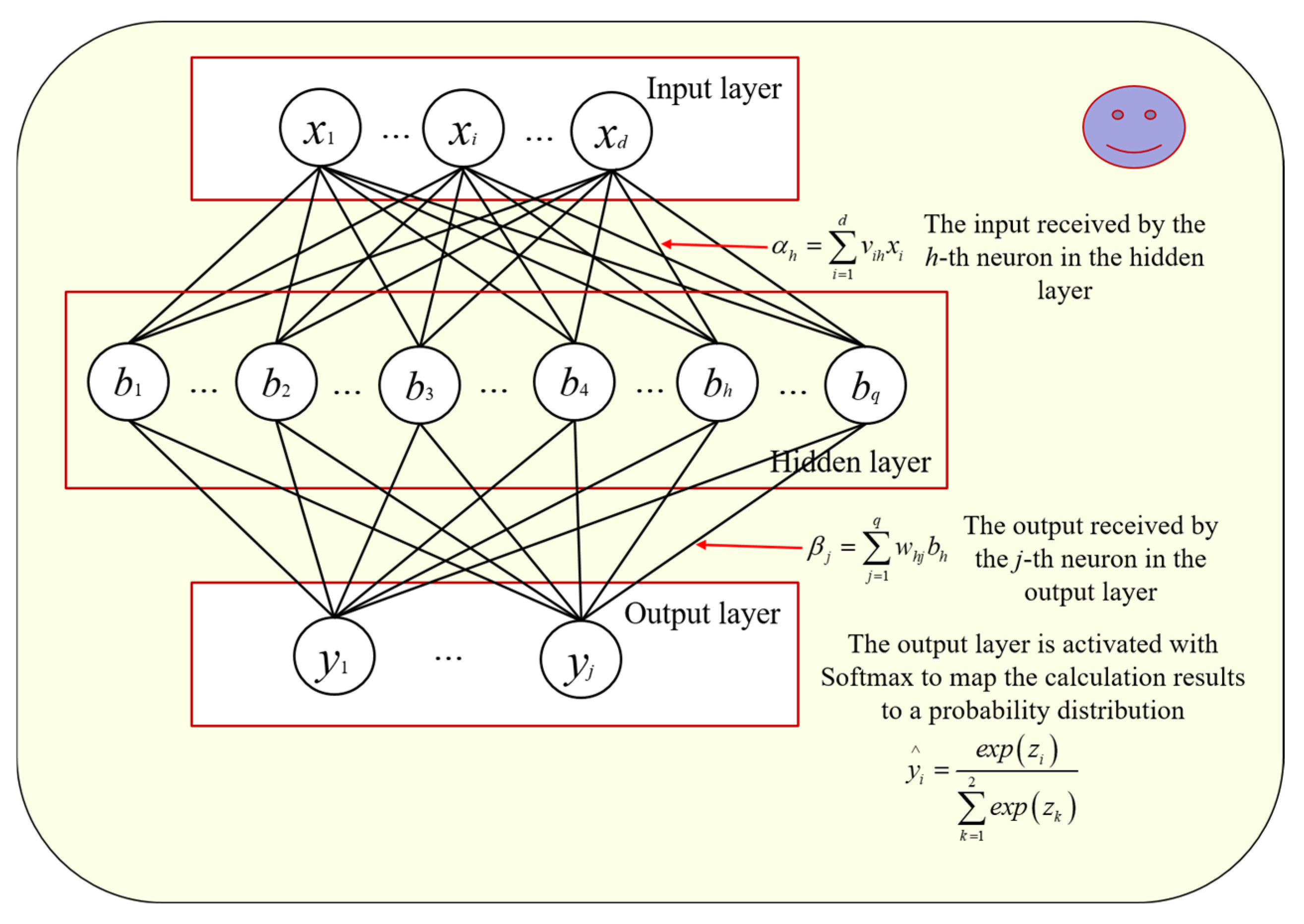
Figure 1. Neural network structure.
Applsci 15 10229 g001
Figure 2. Scatter plot of the distribution of each variable in all of the data.
Applsci 15 10229 g002
Figure 3. Scatter plot of the distribution of each variable in the training dataset.
Applsci 15 10229 g003
Figure 4. Scatter plot of the distribution of each variable in the validation dataset.
Applsci 15 10229 g004
Figure 5. Scatter plot of the distribution of each variable in the test dataset.
Applsci 15 10229 g005
Figure 6. Overall implementation process of the model.
Applsci 15 10229 g006
Figure 7. Calculation of evaluation indicators for the neural network model.
Applsci 15 10229 g007
Figure 8. ROC curve calculation after training.
Applsci 15 10229 g008
Figure 9. Confusion matrix calculation result of the ANN model.
Applsci 15 10229 g009
Figure 10. Borehole profile of Yuanlin-YL-BH-6.
Applsci 15 10229 g010
Figure 11. Calculation results of each method.
Applsci 15 10229 g011
Table 1. Descriptive statistics of data characteristics.
FactorsMwgamax (g)σv (kPa)σv (kPa)ds (m)dw (m)FC (%)D50 (mm)(N1)60
Cases
Liquefaction casesMinimum5.170.0828.84.150.500.000.000.041.10
Maximum8.361.00492.22316.1426.0016.7499.001.6042.70
Mean7.190.35142.1374.556.271.8021.610.2412.04
Standard deviation0.380.17111.7656.095.831.1615.180.225.70
Non-liquefaction casesMinimum5.610.0535.005.340.300.000.000.042.50
Maximum8.360.78363.30257.0031.809.6092.001.6070.50
Mean7.110.27114.1068.137.832.0616.260.2521.17
Standard deviation0.480.17140.3769.897.361.1116.140.2113.83
Table 2. Model performance evaluation indicators calculation.
Evaluation IndicatorsComputing EquationsPerformance Evaluation
Accuracy
(ACC)
ACC = (TP + TN)/(TP + FN + FP + TN)A larger number indicates higher accuracy in prediction
Precision (Pre)Pre = TP/(TP + FP)Restrict each other with Rec
Recall (Rec)Rec = TP/(TP + FN)Restrict each other with Pre
F1F1 = 2Prex × Rec/(Prex + Rec)A larger number indicates that Pre and Rec are better
Table 3. Calculation results under different conditions for the model.
ds (m)Liq (%)N-Liq (%)amax
(g)
Liq (%)N-Liq (%)(N1)60Liq (%)N-Liq (%)
0–1076.3284.000.07–0.13/100.00≤1086.36100.00
10–20100.00100.000.13–0.2466.6784.2110–1584.6266.67
>20/100.000.24–0.4481.8290.0015–3078.9585.71
///0.44–0.83100.00100.00>30/100
Table 4. Misclassified cases of the model.
VariablesMwgamax (g)σv (kPa)σv (kPa)ds (m)dw (m)FC (%)D50 (mm)(N1)60Liq
Number
16.820.1579.1365.444.903.5050.000.093.51Yes
25.280.2386.2248.864.720.9126.200.1111.28Yes
36.820.41133.82111.267.004.7013.000.1920.63Yes
47.260.2442.7931.632.441.307.001.6018.69Yes
56.820.22115.5186.096.003.005.000.3216.38Yes
66.380.1617.7110.381.050.3091.000.013.98Yes
76.380.2086.2248.864.720.9126.200.1111.28Yes
87.370.1448.8630.924.272.443.000.809.31Yes
97.150.35147.74106.347.973.753.290.5020.56Yes
106.930.23112.2270.886.001.7815.000.1517.00No
117.370.18117.8678.646.502.500.000.3614.40No
127.260.2875.8163.794.273.050.000.4117.96No
137.260.2484.0663.144.572.4426.000.1214.92No
Table 5. Comparison results of the discrimination performance for each method.
IndicatorACC
(%)
Pre
(%)
Rec
(%)
F1
(%)
Method
ANN86.1791.8483.3387.38
SVM85.1181.2596.3088.14
LRM70.7466.8097.1979.18
R.B. Seed83.9281.3793.2686.91
NCEER71.0667.0597.1979.36
Idriss81.3590.5475.2882.21
Code method66.5664.8091.0175.70
Principle method79.4289.5872.4780.12
Table 6. The assessment results of each method at different depths.
DepthAll Samples0–20 m>20 m
MethodACC (%)Liq (%)N-Liq (%)ACC (%)Liq (%)N-Liq (%)ACC (%)Liq (%)N-Liq (%)
ANN86.1783.3390.0085.2383.0288.57100.00100.00100.00
SVM85.1196.3070.0083.9196.2364.71100.00100.00100.00
LRM70.7497.1935.3470.6997.0832.7771.43100.0057.14
R.B. Seed83.9283.2671.4385.1792.4074.7966.67100.0050.00
NCEER71.0697.1936.0964.8397.0818.4961.90100.0042.86
Idriss81.3575.2889.4780.6974.8589.0890.4885.7192.86
Code Method66.5691.0166.1783.4590.6473.1038.10100.007.14
Principle Method79.4272.4788.7279.6671.3591.6076.19100.0064.29
Table 7. The specific liquefaction probability prediction results of the ANN model.
Caseds (m) Observed ResultPredicted ResultProbability (%)
119.3LiqLiq94.93
28LiqLiq98.18
34.5LiqLiq99.29
44.9LiqN-Liq9.81
510.3LiqLiq87.00
610.4LiqLiq99.84
73LiqLiq99.10
83LiqLiq99.60
94.7LiqN-Liq48.84
104.3LiqLiq82.40
117LiqN-Liq10.07
124LiqLiq96.90
1312.8LiqLiq79.06
1411.5LiqLiq65.79
156.3LiqLiq95.58
802.5N-LiqN-Liq
816.0N-LiqN-Liq
8225.2N-LiqN-Liq0.00
836.3N-LiqN-Liq0.00
845.2N-LiqN-Liq11.05
856.5N-LiqLiq67.58
863.5N-LiqN-Liq0.22
8728.0N-LiqN-Liq0.01
8816.5N-LiqN-Liq0.00
8914.3N-LiqN-Liq0.00
9016.5N-LiqN-Liq0.03
917.5N-LiqN-Liq7.93
926.5N-LiqN-Liq0.00
935.5N-LiqN-Liq0.00
9425.2N-LiqN-Liq0.01
Table 8. Sunrise chart of the influence degree for each variable in the ANN model liquefaction probability calculation.
FactorSeismic LoadSoil EnvironmentSoil Properties
MwgamaxσvσvdsdwFCD50(N1)60
Percentage (%)13.8414.3714.1713.9413.2913.4013.9112.6920.28
Disclaimer/Publisher’s Note: The statements, opinions and data contained in all publications are solely those of the individual author(s) and contributor(s) and not of MDPI and/or the editor(s). MDPI and/or the editor(s) disclaim responsibility for any injury to people or property resulting from any ideas, methods, instructions or products referred to in the content.