A Deep Learning-Based Plantar Pressure Measurement System for Accurate Foot Arch Index Estimation

Abstract

The medial longitudinal arch is fundamental to weight distribution, balance, and lower limb biomechanics, and its evaluation is important for identifying abnormalities such as flatfoot or high arch. Traditional clinical methods for assessing the foot arch index (FAI) are often constrained by limited accessibility and inconsistent accuracy. To overcome these limitations, this study proposes a deep learning-based plantar pressure measurement system (DLPPMS) designed for accurate and affordable static foot arch evaluation. The system integrates two resistive pressure sensor arrays combined into a 24 × 24 matrix to acquire plantar pressure data in real time. To enhance spatial resolution and improve the fidelity of pressure distribution, Bessel interpolation is employed to generate smooth, high-resolution plantar pressure maps. Deep learning-based pose estimation and instance segmentation models are further applied to isolate the plantar region and identify anatomical keypoints relevant for FAI computation. The system was validated on participants with flatfoot, normal arch, and high arch conditions, demonstrating high segmentation accuracy, reliable keypoint localization, and consistent FAI estimation with minimal error compared to reference values. These results confirm that the DLPPMS provides accurate, repeatable, and low-cost assessment of the medial longitudinal arch under static conditions. Overall, this work highlights the potential of combining pressure sensing, interpolation algorithms, and deep learning into a portable and scalable system, offering promising applications not only for clinical diagnostics but also for biomechanical research, preventive healthcare, and rehabilitation monitoring.

1. Introduction

The human foot is a complex anatomical structure that plays a crucial role in maintaining balance and facilitating mobility. Based on the height of the medial longitudinal arch, it is typically categorized into three primary types: high arch, normal arch, and low arch [1,2]. Such classification is clinically significant, as deviations from a neutral foot type, such as flatfoot or high arch, have been linked to various musculoskeletal and lower-extremity injuries. Previous studies indicate that aberrant foot structures alter plantar pressure distribution and may increase the risk of injuries, including knee pain, ankle sprains, and stress fractures [3,4,5,6]. For instance, individuals with low arches exhibit elevated plantar pressure in the midfoot area when standing, potentially predisposing them to midfoot collapse and related complications [3,4]. Furthermore, foot misalignment, such as excessive pronation or supination, has been associated with knee and back pain, underscoring the importance of foot posture assessment in both clinical and athletic contexts [5].

Foot posture significantly influences biomechanics, shaping gait patterns, weight distribution, and injury susceptibility. Variations in foot posture, such as pes planus and pes cavus, can affect plantar pressure distribution and gait dynamics. Studies have demonstrated that foot type influences muscle strength and pressure distribution, resulting in distinct biomechanical adaptations [6]. Among various morphological indicators of foot structure, the foot arch index (FAI) is widely recognized due to its simplicity and strong correlation with clinical benchmarks such as navicular height [7]. However, accurate estimation of FAI remains challenging, particularly under static conditions, due to limitations in sensor resolution and segmentation precision. These constraints necessitate more robust computational techniques for improving measurement fidelity, which motivates the development of advanced plantar pressure analysis systems.

Conventional gold-standard systems, such as force plates and podoscopes, provide important benchmarks for foot assessment. Force plates enable accurate dynamic gait analysis but are costly and unsuitable for routine static evaluation, while podoscopes are inexpensive but largely qualitative and poorly standardized. The proposed DLPPMS addresses these limitations by providing a low-cost, portable, and quantitative system for static FAI estimation, offering greater precision and repeatability than podoscopes and improved accessibility compared with force plates.

In recent years, artificial intelligence has emerged as a powerful tool in foot health monitoring, enabling automated analysis of plantar pressure patterns and foot posture. Numerous studies have demonstrated that AI-driven models can classify foot types, detect abnormal gait, and support early diagnosis of conditions such as flatfoot and supination [8,9,10]. Zhao et al. [8] proposed a deep learning approach combining an improved YOLOv5 architecture with attention mechanisms and a multilabel ResNet-50 classifier to identify flatfoot from plantar pressure images. Domínguez-Morales et al. [9] developed a smart insole system integrated with a real-time neural network that classifies foot posture into pronation, supination, and neutral types based on dynamic plantar pressure data collected during gait. Özateş et al. [10] implemented a machine learning pipeline using models such as k-nearest neighbors and random forest, enhanced by explainable AI techniques like local interpretable model-agnostic explanations, to classify six types of foot conditions, including planovalgus and cavovarus, based on gait kinematic features.

Plantar pressure measurement systems are generally classified into two main types: platform-based systems and in-shoe systems [11]. Compared with in-shoe systems, platform-based systems offer higher spatial resolution and greater measurement stability under static conditions, making them especially suitable for research scenarios requiring detailed plantar pressure analysis. Hence, this study utilizes a platform-based system for plantar pressure data collection. These systems gather plantar pressure data via sensors embedded in a flat surface, enabling high-resolution measurements ideal for assessing plantar pressure distribution with precision. In a recent example, Zheng et al. [12] introduced an automated FAI measurement technique that employs a flexible membrane pressure sensor in conjunction with image processing for noise removal. Similarly, Chae et al. [13] applied a platform-based system combined with deep learning to classify foot types, emphasizing the role of artificial intelligence in enhancing objectivity and diagnostic efficiency. With the rapid evolution of machine learning and deep learning, computer vision techniques have become pivotal for improving plantar pressure analysis and foot classification [14,15]. Among various deep learning techniques, the You Only Look Once (YOLO) series has emerged as one of the most widely adopted object detection frameworks due to its one-stage architecture, which allows classification and localization in a single forward pass, significantly reducing inference latency. Unlike two-stage detectors such as Faster R-CNN, YOLO offers a favorable balance between accuracy and computational efficiency, making it highly suitable for real-time applications on embedded devices. Recent studies have further validated its portability, including walnut detection with YOLOv11 on UAV edge platforms [16], rice panicle detection with YOLOv8n on Raspberry Pi 5 [17], and infrared target detection using Edge-YOLO on RK3588 devices [18]. Based on these advantages, this study adopts YOLOv11n for plantar region segmentation and anatomical keypoint detection within the proposed DLPPMS.

However, the spatial resolution of sensors constrains the precision of plantar pressure measurements. Interpolation is a numerical technique used to estimate unknown values between discrete data points. B-spline interpolation and Bessel interpolation both enhance the resolution and continuity of data representations while maintaining geometric structures and visual quality [19,20,21]. B-spline interpolation is widely adopted in computer graphics and image processing due to its high smoothness and strong local control, making it particularly suitable for curve and surface reconstruction [20,21]. In contrast, Bessel interpolation leverages the mathematical properties of Bessel functions, especially their well-defined boundary behavior and oscillatory characteristics, to preserve fine details and edge features. This makes it especially effective in tasks that require smooth extension and structural fidelity [22].

While these techniques contribute to improving data resolution and structural accuracy, it remains essential to validate the overall performance of the proposed system. Thus, this study employs the footprint imaging measurement (FIM) method as a benchmark for comparison. Traditional ink-based footprint techniques are often labor-intensive and difficult to standardize due to manual procedures [23]. To address these limitations, this study utilizes the VERS MP-5 pressure-sensitive footprint device, which captures high-quality plantar contact images without the need for ink, offering greater measurement consistency and operational convenience. Based on prior discussion, this study employs a platform-type deep learning-based plantar pressure measurement system (DLPPMS) combined with YOLOv11n for foot axis detection and sole segmentation to enhance the accuracy of the FAI calculation. However, the limited spatial resolution of the sensors constrains the precision of pressure measurements. In order to address this issue, numerical interpolation techniques are incorporated to reconstruct a more continuous and detailed pressure distribution. This approach yields more complete and accurate data, thereby supporting more robust biomechanical and clinical analyses.

The novelty of this study lies in demonstrating that accurate and repeatable foot arch classification can be achieved under sparse sensing conditions by combining deep learning and interpolation techniques on a compact embedded platform. The main contributions are as follows: (1) design and implementation of the DLPPMS as an in-house foot arch classification framework integrating resistive sensing, image-based analysis, and automated FAI estimation; (2) integration of YOLOv11n-based keypoint detection and Bessel interpolation to enhance accuracy under low-resolution conditions; and (3) full local execution of the entire pipeline, from data acquisition to FAI computation, on a resource-constrained Raspberry Pi Zero 2 W, confirming the feasibility of low-cost embedded deployment.

The remainder of this paper is organized as follows. Section 2 details the hardware architecture of the proposed DLPPMS, including the sensor arrays and signal acquisition circuit. Section 3 introduces the algorithmic methodology, encompassing preprocessing, interpolation, pose estimation, segmentation, and FAI estimation. Section 4 presents the experimental results and discusses the performance of the system in comparison with conventional methods. Finally, Section 5 concludes the study and outlines potential applications.

2. Hardware Architecture of the DLPPMS

The proposed DLPPMS adopts a platform-type architecture and comprises a Raspberry Pi Zero for data processing, a Raspberry Pi Pico for sensor control, two 12 × 24 resistive pressure sensor arrays, with one assigned to the left foot and the other to the right foot, seamlessly combined into a 24 × 24 pressure-sensing matrix, a custom signal acquisition circuit, and a display module, as illustrated in Figure 1. 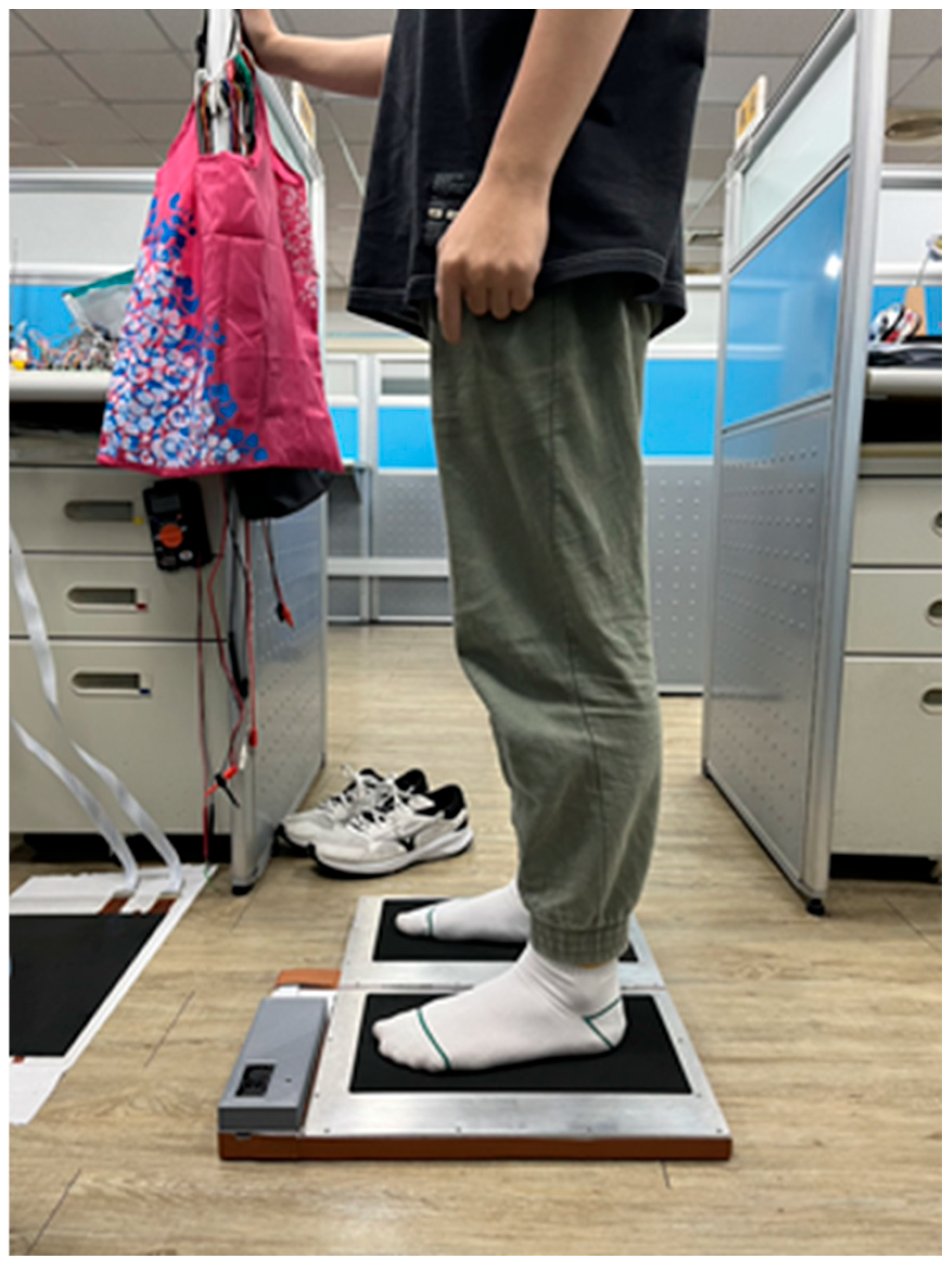Figure 2 presents a schematic illustration of a participant standing on the system during measurement.

Each pressure-sensing unit consists of a flexible conductive layer, an insulating spacer, and a pair of electrodes. In the absence of external load, the spacer maintains a separation between the electrodes, resulting in an open-circuit state, as illustrated in Figure 3a. Under applied pressure, the conductive layer undergoes compression, enabling electrical contact between the electrodes and thereby closing the circuit, as shown in Figure 3b. Each sensor element has a diameter of 10 mm, with an inter-element spacing of 3 mm vertically and 5 mm horizontally, facilitating high-resolution plantar pressure acquisition for foot arch index (FAI) estimation.

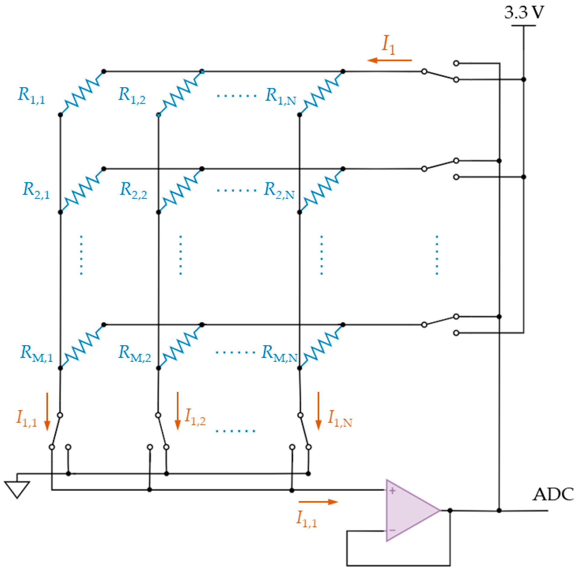
Pressure signals acquired from the resistive pressure sensor array are transmitted through a dedicated signal acquisition circuit and converted into digital form by the onboard analog-to-digital converter (ADC) of the Raspberry Pi Pico. The schematic diagram of the signal acquisition system is shown in Figure 4. This architecture employs a multiplexer-based switching mechanism that sequentially selects individual sensor elements using a row and column addressing scheme, allowing for precise voltage sampling. The digitized signals are then communicated to the Raspberry Pi Zero through a universal asynchronous receiver and transmitter interface. The Raspberry Pi Zero functions as the primary processing unit of the proposed DLPPMS, performing critical computational tasks such as Bessel and B-spline interpolation, pose estimation, and instance segmentation based on the YOLOv11n model, and the final calculation of the FAI.

3. Methodology

The algorithmic architecture of the proposed DLPPMS is designed to process raw sensor signals and enable accurate estimation of the FAI through a structured computational pipeline. This methodology consists of sequential stages, including data preprocessing, principal component analysis (PCA)-based alignment, image interpolation, pose estimation, and instance segmentation. Each stage enhances the geometric coherence and numerical precision of plantar pressure maps, thereby improving the overall accuracy of the analysis. Figure 5 illustrates an overview of the complete system workflow, covering Web BLE communication, sensor data acquisition, signal validation, pressure map construction, alignment, segmentation, and FAI estimation. 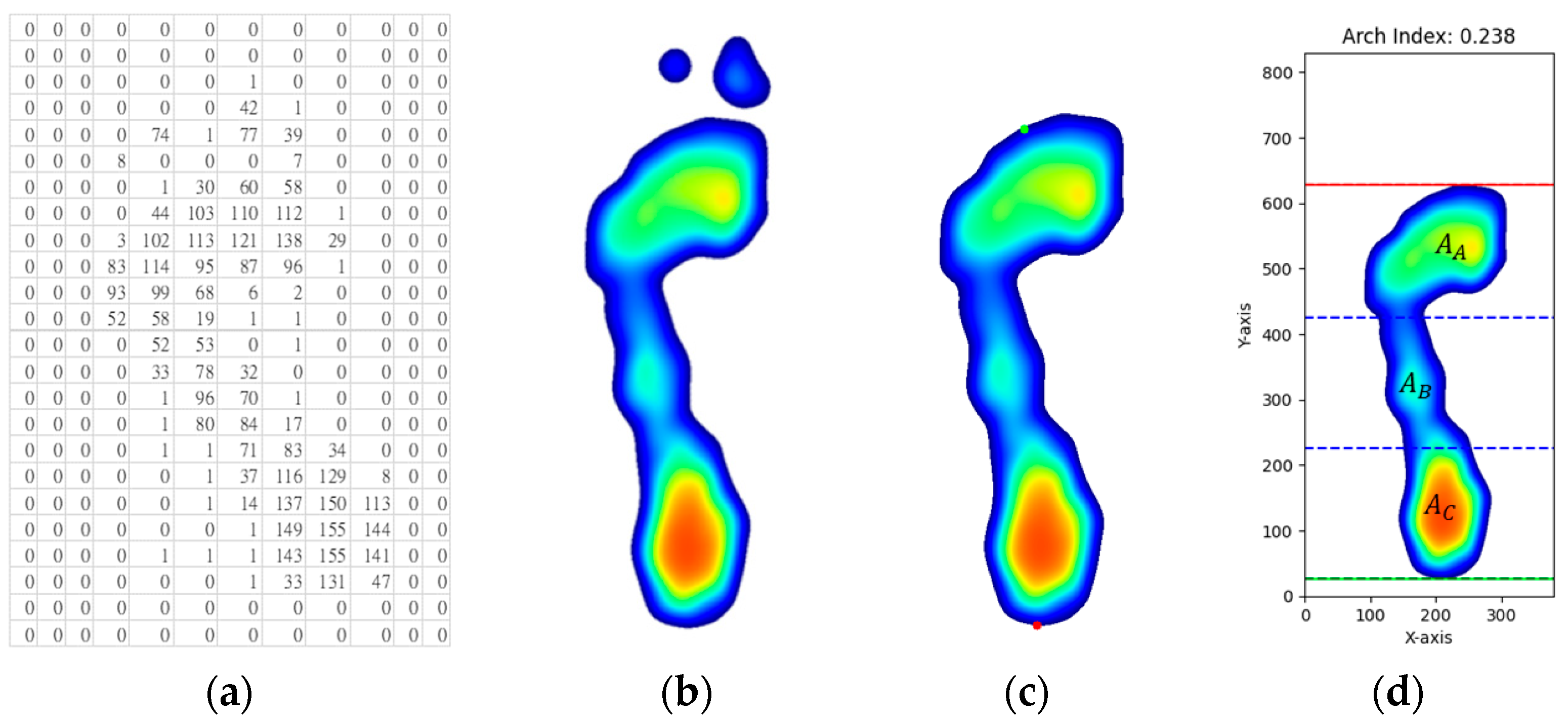Figure 6 summarizes the transformation from raw input to anatomically structured output. The raw pressure matrix acquired from the resistive sensor array is depicted in Figure 6a. The interpolated plantar pressure image after PCA-based alignment is shown in Figure 6b. The anatomically aligned and segmented plantar region with irrelevant areas removed is presented in Figure 6c. Its division into three equal parts for FAI estimation is illustrated in Figure 6d. The DLPPMS achieves real-time performance by combining efficient hardware and lightweight algorithms. Sensor data are acquired and transmitted to the Raspberry Pi Zero, where interpolation and YOLO-based processing are executed within seconds, enabling immediate visualization of plantar pressure distribution and FAI values. Such real-time feedback is particularly important in clinical contexts, as it allows rapid assessment and decision-making without the need for offline data processing. The algorithmic components comprising the DLPPMS pipeline are detailed in the following subsections.

3.1. Principal Component Analysis (PCA) Based Alignment

During static stance, certain participants exhibited noticeable foot rotation patterns, such as in-toeing or out-toeing, leading to orientation deviations in the captured plantar pressure images. These deviations can negatively impact the accuracy of YOLO-based keypoint detection, particularly when locating anatomical landmarks such as the heel and the base of the second toe. To address this issue, this study applies PCA for spatial alignment. PCA examines the distribution of non-zero pressure pixels to determine the direction of maximum variance, thereby identifying the principal axis of the foot. The pressure image is then rotated along this axis to achieve vertical alignment across all samples. Unlike methods requiring explicit foot boundary detection, PCA offers a global statistical approach that is resilient to low resolution, sensor noise, and partial occlusion. It enables reliable orientation estimation based solely on the spatial distribution of pressure data. Furthermore, PCA is computationally efficient and broadly applicable to diverse foot morphologies. This alignment process improves the consistency of plantar pressure representations, thereby enhancing the robustness and accuracy of subsequent anatomical landmark detection and FAI estimation [24]. Let the set of non-zero pressure coordinates X be defined as follows [25]:

$$\mathbf{X}={\left\{\left(x_i, y_i\right)\right\}}_{i=1}^n$$

(1)

where $x_i$ and $y_i$ represent the horizontal and vertical coordinates of the i-th non-zero pressure point, and $n$ denotes the total number of such points. To eliminate translational bias, the coordinates are mean-centered as follows:

$$\overline{x}={\displaystyle \frac{1}{n}}\sum _{i=1}^n{x}_i, \overline{y}={\displaystyle \frac{1}{n}}\sum _{i=1}^n{y}_i$$

(2)

$${\mathbf{X}}_{\mathbf{C}}={\left\{\right(x_i-\overline{x},{ y}_i-\overline{y}\left)\right\}}_{i=1}^n$$

(3)

The mean-centered dataset ${\mathbf{X}}_{\mathbf{C}}$ is then used to compute the covariance matrix $\mathbf{\Sigma }$∈ R^2×2 as follows:

$$\mathbf{\Sigma }={\displaystyle \frac{1}{n-1}}\sum _{i=1}^n\left[\begin{array}{c}{x}_i-\overline{x}\\ y_i-\overline{y}\end{array}\right]\left[\begin{array}{cc}{x}_i-\overline{x}& y_i-\overline{y}\end{array}\right]=\left[\begin{array}{cc}Var\left(x\right)& Cov(x,y)\\ Cov(x,y)& Var\left(y\right)\end{array}\right]$$

(4)

where $\mathrm{V}\mathrm{a}\mathrm{r}\left(x\right)$ and $\mathrm{V}\mathrm{a}\mathrm{r}\left(y\right)$ denote the variances along the horizontal and vertical axes, respectively, and $\mathrm{C}\mathrm{o}\mathrm{v}(x,y)$ represents the covariance between them.

To identify the direction of maximum variance, the eigenvalues of the covariance matrix Σ are derived by solving its characteristic equation:

$$\det \left(\mathbf{\Sigma }-\lambda \mathit{I}\right)=0$$

(5)

which expands into the quadratic form:

$${\lambda }^2-\left({\sigma }_{xx}+{\sigma }_{yy}\right)\lambda +\left({\sigma }_{xx}{\sigma }_{yy}-{\sigma }_{xy}^2\right)=0$$

(6)

where ${\sigma }_{xx}$ is the $\mathrm{V}\mathrm{a}\mathrm{r}\left(x\right)$, ${\sigma }_{yy}$ is the $\mathrm{V}\mathrm{a}\mathrm{r}\left(y\right)$, and ${\sigma }_{xy}$ is the $\mathrm{C}\mathrm{o}\mathrm{v}(x,y)$. Solving this equation yields two real eigenvalues, ${\lambda }_1$≥${\lambda }_2$, corresponding to the variances along the principal and secondary axes, respectively. The eigenvector associated with the larger eigenvalue λ₁ defines the orientation of the principal axis, which is subsequently used for spatial alignment of the plantar pressure image.

The principal axis vector ${\mathit{v}}_1$∈ R² is obtained by solving the following homogeneous linear system:

$$\left(\mathbf{\Sigma }-{\lambda }_1\mathit{I}\right){\mathbf{v}}_1=0$$

(7)

Let ${\mathit{v}}_1=\left[\begin{array}{c}{v}_x\\ v_y\end{array}\right]$, where $v_x$ and $v_y$ denote the horizontal and vertical components of the eigenvector, respectively. To achieve vertical alignment of the foot image, the angular deviation $\theta$ between the principal axis and the vertical axis is calculated using the two-argument arctangent function:

$$\theta ={\mathit{tan}}^{-1}\left({\displaystyle \frac{v_y}{v_x}}\right)$$

(8)

Each plantar pressure image is then rotated by $\theta$ to align the principal axis with the vertical orientation. This alignment step not only ensures visual consistency across participants but also significantly enhances the accuracy of subsequent keypoint detection. Without such preprocessing, YOLO-based pose estimation models are prone to performance degradation due to rotational variance in the input data.

3.2. Bessel and B-Spline Interpolation

Bessel interpolation was selected for its advantageous characteristics in preserving local anatomical features and minimizing abrupt intensity transitions. As a type of radial basis function interpolation, it estimates unknown pressure values by calculating distance-weighted contributions from surrounding known points. The interpolation kernel is derived from the zeroth-order Bessel function of the first kind, which exhibits oscillatory behavior. This high-frequency sensitivity is particularly effective in retaining fine-scale pressure gradients and structural nuances in the reconstructed plantar pressure map. The mathematical formulation and kernel behavior are detailed in the following section.

3.2.1. Bessel Interpolation

Bessel interpolation is a radial basis function technique that employs the zeroth-order Bessel function of the first kind $J_0\left(z\right)$, as its interpolation kernel. This function exhibits radial symmetry and oscillatory behavior, with amplitudes that gradually attenuate with increasing distance. The analytical expression of $J_0\left(z\right)$ is defined by the following integral form [26]:

$$J_0(z)={\displaystyle \frac{1}{2\pi }}{\int }_0^{2\pi }cos(z\mathit{sin}\theta )d\theta$$

(9)

In two-dimensional interpolation scenarios, the estimated value at a location $\left(x,y\right)$ is computed as a weighted sum of nearby sampled values $f\left(i+m, j+n\right)$, where the weights are determined by the Euclidean distance between the sample locations and the interpolation point. The interpolation formula is given by the following [27]:

$$f\left(x,y\right)\approx {\sum }_{m=-M}^M{\sum }_{n=-N}^N{J}_0\left[\alpha ·\sqrt{{\left(x_r-i-m\right)}^2+{(y_r-j-n)}^2}·f\left(i+m, j+n\right)\right]$$

(10)

where $\left(x_r,y_r\right)$ denotes the nearest integer grid point to the target location $\left(x,y\right)$, and $\alpha$ is a scaling parameter that modulates the spatial decay rate of the Bessel kernel. The parameters $M$ and $N$ define the neighborhood window along the horizontal and vertical axes, respectively. By applying a distance-weighted average based on the Bessel kernel, this method effectively suppresses aliasing artifacts and mitigates abrupt intensity transitions, thereby enhancing gradient continuity and preserving fine structural details in the reconstructed plantar pressure image.

3.2.2. B-Spline Interpolation

B-spline interpolation is a piecewise polynomial technique designed to achieve smooth, locally controlled transitions between data points. The zeroth-order B-spline basis function $B_{i,0}\left(x\right)$ is defined as follows:

$$B_{i,0}\left(x\right)=\left\{\begin{array}{cc}1,& t_i\le x<t_{i+1}\\ 0,& \mathrm{o}\mathrm{t}\mathrm{h}\mathrm{e}\mathrm{r}\mathrm{w}\mathrm{i}\mathrm{s}\mathrm{e}\end{array}\right.$$

(11)

This function is a piecewise constant representation that equals 1 over a specific knot interval and zero elsewhere. For B-splines of order $k$ > 0, the basis functions are defined recursively using a weighted combination of two lower-order B-splines [28]:

$$B_{i,k}\left(x\right)={\displaystyle \frac{x-t_i}{t_{i+k}-t_i}}{B}_{i,k-1}\left(x\right)+{\displaystyle \frac{t_{i+k+1}-x}{t_{i+k+1}-t_{i+1}}}{B}_{i+1, k-1}\left(x\right)$$

(12)

where $t_i$ denotes the elements of the knot vector and $k$ is the spline order. This recursive formulation ensures that the basis functions possess compact support and exhibit continuity up to C^k−1, meaning that the function and its derivatives up to order $k$ − 1 are continuous. For example, a cubic B-spline (i.e., $k$ = 3) maintains C² continuity, offering smooth first- and second-order derivatives at segment boundaries.

In two-dimensional interpolation, a B-spline surface is constructed as a tensor product of one-dimensional basis functions along the $x$ and $y$ directions. Let $P_{i,j}$ denote the control point values (e.g., pressure measurements), and $B_{i,k}\left(x\right)$, $B_{j,l}\left(y\right)$ represent the respective B-spline basis functions in each dimension with degrees $k$ and $l$. The interpolated surface $S\left(x,y\right)$ is defined as

$$S\left(x,y\right)=\sum _{i=0}^d\sum _{j=0}^g{P}_{i,j}·B_{i,k}\left(x\right)·B_{j,l}(y)$$

(13)

where d and g denote the number of control points along the $x$ and $y$ directions, respectively. This formulation provides efficient and smooth two-dimensional interpolation across a grid, ensuring both high-order continuity and local adaptability in the reconstructed surface. The effective support of each basis function determines the number of neighboring control points influencing a given interpolated value. In visualization contexts, filters such as spline16 adopt wider cubic B-spline kernels to enhance smoothness by incorporating broader neighborhoods. Moreover, the choice between uniform and non-uniform knot vectors, as well as appropriate boundary conditions, significantly affects the overall shape and smoothness of the interpolated surface.

3.3. Deep Learning YOLO Models for Image Processing

A total of 700 plantar pressure images were acquired, encompassing both left and right feet under natural bipedal standing conditions. The dataset was partitioned into 500 images for training, 100 images for validation, and 100 images for testing. All images were manually annotated with key anatomical landmarks and plantar boundaries to support supervised learning. These annotated datasets were utilized to train and evaluate deep learning models for pose estimation and instance segmentation, forming a critical component of the DLPPMS pipeline. The integration of YOLO-based models enabled precise detection of foot orientation, heel position, and toe landmarks, which are essential for accurate FAI estimation.

3.3.1. Pose Estimation for Foot Alignment (YOLOv11n-Pose)

As a key component of the DLPPMS, the YOLOv11n-pose model was implemented to detect two critical anatomical keypoints: the base of the second toe and the center of the heel. These keypoints enable image alignment via rotation correction, thereby enhancing the geometric consistency of plantar pressure maps and improving the accuracy of FAI estimation. The model was trained on a custom-labeled dataset comprising manually annotated keypoints for supervised learning.

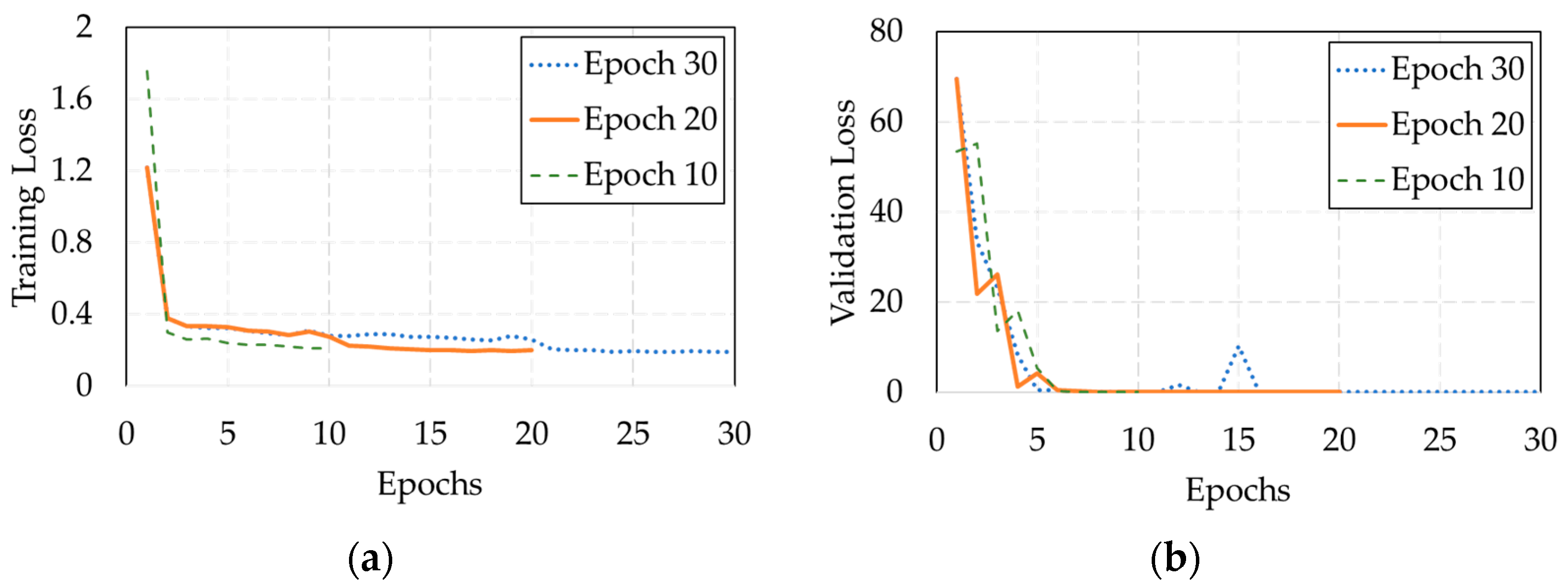
To assess how training duration influences model performance, three experiments were conducted with training epochs set to 10, 20, and 30, while keeping all other configurations constant. The training process utilized the AdamW optimizer with an initial learning rate of 0.001, a batch size of 32, and input images sized at 640 × 320 pixels. A cosine annealing schedule was applied to adjust the learning rate dynamically, with a weight decay of 0.0005 and three warm-up epochs to stabilize early learning. Automatic mixed precision (AMP) was enabled to improve computational efficiency on a GPU (NVIDIA T4 via Google Colab, Mountain View, CA, USA).

The training and validation loss curves for the three epoch settings are shown in Figure 7. Among the models, the 20-epoch model demonstrated the most favorable balance between convergence speed and generalization performance. It exhibited rapid initial convergence, followed by a stable reduction in loss, ultimately achieving a lower final validation loss than both the 10-epoch and 30-epoch models. Although the 30-epoch model achieved a comparable final loss, it showed minimal performance gains beyond 20 epochs. These findings suggest that 20 epochs are sufficient for achieving robust and accurate keypoint localization under the given training conditions. Accordingly, the 20-epoch model was adopted for all subsequent pose estimation tasks in this study.

The accuracy of keypoint localization was evaluated using the root mean square error (RMSE) metric [29], defined as follows:

$$\mathrm{R}\mathrm{M}\mathrm{S}\mathrm{E}=\sqrt{{\displaystyle \frac{1}{N}}\sum _{i=1}^N\left[{\left(x_i-{\widehat{x}}_i\right)}^2+{\left(y_i-{\widehat{y}}_i\right)}^2\right]}$$

(14)

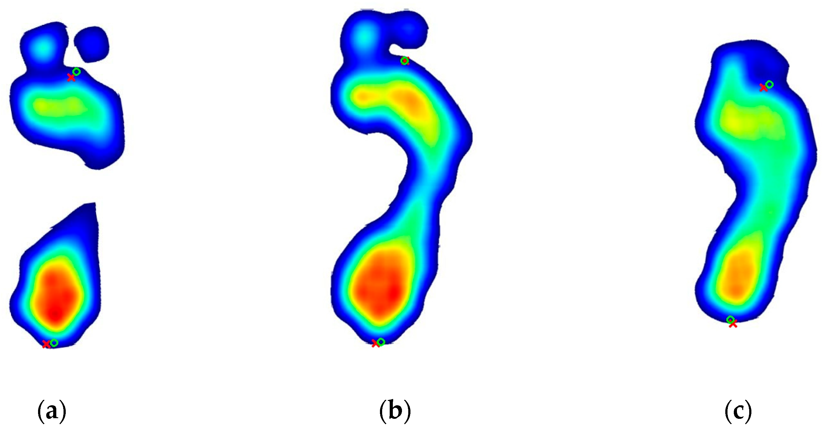
where ($x_i,y_i$) denote the ground-truth coordinates, (${\widehat{x}}_i,{\widehat{y}}_i$) are the corresponding predicted keypoints, and $N$ is the total number of keypoints evaluated. The proposed YOLOv11n-pose model achieved an RMSE of 3.8 mm, demonstrating high precision in anatomical landmark localization. Figure 8 illustrates a visual comparison between the predicted keypoints and the corresponding ground-truth annotations across three foot arch types: high, normal, and flat.

Once the two anatomical keypoints were identified, the angular deviation between the foot’s orientation and the vertical axis was computed to perform alignment correction. Let ($x_1$, $y_1$) denote the coordinates of the heel and ($x_2$, $y_2$) the base of the second toe. The rotation angle θ between the line connecting these two points and the vertical direction was calculated as

$${\theta }_c={\mathrm{t}\mathrm{a}\mathrm{n}}^{-1}\left({\displaystyle \frac{x_2-x_1}{y_2-y_1}}\right)$$

(15)

The ${\theta }_c$ represents the inclination of the foot with respect to the vertical axis. To standardize the orientation, the entire image was rotated counterclockwise by $-{\theta }_c$ degrees, aligning the two keypoints along a common vertical line. This alignment procedure effectively compensates for rotational variance during data acquisition and significantly improves the consistency and reliability of subsequent FAI estimations.

3.3.2. Instance Segmentation for Plantar Region (YOLOv11n-Seg)

To enhance the precision of FAI estimation, the YOLOv11n-seg model was implemented to perform instance segmentation of the plantar region by excluding the toe area. This refinement of the region of interest ensures that FAI calculations are restricted to the anatomically relevant midfoot and hindfoot zones. The model was trained on a custom-labeled dataset containing manually annotated plantar boundaries.

To explore the relationship between training duration and segmentation accuracy, three training configurations with epoch settings of 10, 20, and 30 were tested under consistent experimental conditions. The model was trained using the AdamW optimizer (learning rate: 0.001), with a batch size of 32 and an input resolution of 640 × 320 pixels. A cosine learning rate scheduler and a weight decay of 0.0005 were adopted, along with three warm-up epochs to promote training stability. To accelerate computation, AMP was employed on an NVIDIA T4 GPU hosted on Google Colab.

The training and validation loss curves for each epoch setting are presented in Figure 9. Among these, the 10-epoch model demonstrated the optimal balance between training speed and segmentation accuracy. It achieved rapid early convergence, a stable loss decline, and the lowest final validation loss with minimal fluctuation. While the 20- and 30-epoch models exhibited similar final losses, no notable improvement was observed beyond 10 epochs. These results suggest that 10 epochs provide sufficient capacity for robust and accurate segmentation under the current configuration, with segmentation outputs exemplified in Figure 10.

Segmentation accuracy was evaluated using the intersection over union (IoU) metric [30], which quantifies the ratio between the area of overlap and the area of union between the predicted region P and the ground truth Q. As each input image contains a single plantar region and the model outputs a corresponding mask, the evaluation reduces to a binary classification per sample. At a given IoU threshold, t, a prediction is classified as a true positive if the IoU exceeds t; otherwise, it is treated as a false negative. Since only one prediction is produced per image, false positives are excluded from the evaluation. Accordingly, the average precision at each threshold $\mathrm{A}{\mathrm{P}}_{\mathrm{t}}$ assumes a value of either 1 or 0, and the final average is computed across all samples.

Two commonly adopted metrics were used: $\mathrm{A}{\mathrm{P}}_{50}$, representing the average precision at an IoU threshold of 50%, and $\mathrm{A}{\mathrm{P}}_{50:5:95}$, representing the mean average precision across ten IoU thresholds ranging from 50% to 95% in 5% increments, calculated as follows:

$$\mathrm{A}{\mathrm{P}}_{50:5:95}={\displaystyle \frac{1}{10}}\sum _{\mathrm{t}\in \mathbf{T}}\mathrm{A}{\mathrm{P}}_{\mathrm{t}}$$

(16)

where T is the set of IoU thresholds {50%, 55%, …, 95%}.

In this study, the YOLOv11n-seg model achieved an $\mathrm{A}{\mathrm{P}}_{50}$ of 0.99 and an $\mathrm{A}{\mathrm{P}}_{50:5:95}$ of 0.98, demonstrating high segmentation accuracy across varying thresholds. The resulting segmentation masks reliably exclude the toe regions, thereby ensuring that only the relevant plantar surface is retained for subsequent pressure map analysis and FAI estimation.

3.4. Foot Arch Index Estimation

Following keypoint detection and instance segmentation, the plantar pressure distribution is analyzed to estimate the FAI, a well-established quantitative metric for classifying foot arch morphology. The FAI quantifies the proportion of midfoot contact area relative to the total plantar surface area, excluding the toes. In this study, the segmented plantar region is partitioned longitudinally into three equal sections: the forefoot, midfoot, and heel, as shown in Figure 6d. The FAI value is calculated as follows:

$$\mathrm{F}\mathrm{A}\mathrm{I}={\displaystyle \frac{A_B}{A_A+A_B+A_C}}$$

(17)

where $A_A$, $A_B$, and $A_C$ denote the contact areas of the forefoot, midfoot, and heel, respectively. Based on established thresholds, an FAI value below 0.21 indicates a high arch, values between 0.21 and 0.26 represent a normal arch, and values greater than 0.26 are indicative of flatfoot. This standardized estimation method enables objective evaluation of foot structure from static plantar pressure data, thereby supporting applications in both biomechanical analysis and clinical assessment.

3.5. Comparative Method Using the FIM Method

To assess the validity of the proposed DLPPMS, this study employs the FIM method as a comparative reference standard. The FIM procedure utilizes the VERS MP-5 pressure-sensitive footprint device to capture high-resolution static plantar images, providing a reliable basis for FAI estimation. In the FIM-based measurement procedure, the participant stands on one foot on the MP-5 pressure-sensitive platform, ensuring full plantar contact with the sensing plate to generate a static plantar pressure map, as shown in Figure 11a. After image acquisition, researchers manually delineate the plantar region by tracing the boundary of the visible sole, excluding the toes and surrounding background, and manually aligning the image, as illustrated in Figure 11b. The refined contact region is then used to compute the FAI, as depicted in Figure 11c. The FAI values obtained through the FIM method are compared with those derived from the DLPPMS to evaluate measurement accuracy, consistency, and suitability for clinical and research applications.

In summary, the proposed DLPPMS emphasizes not only functional implementation but also low cost, portability, and clinical feasibility. The 24 × 24 sensor matrix balances spatial resolution with circuit complexity, while numerical methods and deep learning compensate for hardware limitations. This design ensures stability and accuracy even on embedded platforms, thereby laying a solid foundation for subsequent experimental validation.

4. Experimental Results and Discussion

To evaluate the accuracy and consistency of FAI estimation using the proposed DLPPMS, which incorporates both Bessel and B-spline interpolation techniques, a comparative assessment was conducted against the conventional FIM method. Three male participants with distinct foot arch types were recruited: a 24-year-old with flatfoot, a 21-year-old with a normal arch, and a 24-year-old with a high arch. All participants were instructed to maintain a natural upright standing posture during measurement to ensure standardized loading conditions. For each participant, FAI values were computed using both interpolation techniques under the DLPPMS and the conventional FIM method. The corresponding experimental results are summarized in

Table 1. Foot arch index (FAI) measurements for the flatfoot group using three different techniques.

Foot Arch Index	DLPPMS (Bessel)		DLPPMS (B-Spline)		FIM
	Left Foot	Right Foot	Left Foot	Right Foot	Left Foot	Right Foot
Measurement 1	0.319	0.304	0.308	0.304	0.327	0.318
Measurement 2	0.317	0.306	0.313	0.303	0.329	0.300
Measurement 3	0.319	0.308	0.310	0.300	0.333	0.304
Measurement 4	0.320	0.308	0.314	0.298	0.330	0.297
Measurement 5	0.320	0.305	0.310	0.302	0.307	0.309
Measurement 6	0.318	0.305	0.310	0.301	0.330	0.317
Measurement 7	0.318	0.308	0.314	0.304	0.326	0.301
Measurement 8	0.322	0.306	0.312	0.302	0.292	0.306
Measurement 9	0.320	0.306	0.316	0.305	0.307	0.311
Measurement 10	0.322	0.305	0.313	0.304	0.316	0.299
Average	0.320	0.306	0.312	0.302	0.320	0.306

,

Table 2. Foot arch index (FAI) measurements for the normal arch group using three different techniques.

Foot Arch Index	DLPPMS (Bessel)		DLPPMS (B-Spline)		FIM
	Left Foot	Right Foot	Left Foot	Right Foot	Left Foot	Right Foot
Measurement 1	0.244	0.224	0.241	0.226	0.235	0.242
Measurement 2	0.243	0.223	0.240	0.224	0.254	0.232
Measurement 3	0.242	0.226	0.241	0.228	0.241	0.235
Measurement 4	0.242	0.226	0.242	0.228	0.253	0.235
Measurement 5	0.243	0.224	0.244	0.223	0.235	0.241
Measurement 6	0.242	0.227	0.244	0.224	0.249	0.222
Measurement 7	0.245	0.226	0.241	0.223	0.240	0.227
Measurement 8	0.246	0.227	0.246	0.224	0.246	0.214
Measurement 9	0.245	0.226	0.245	0.224	0.248	0.210
Measurement 10	0.244	0.226	0.244	0.223	0.237	0.208
Average	0.244	0.226	0.243	0.225	0.244	0.226

and

Table 3. Foot arch index (FAI) measurements for the high arch group using three different techniques.

Foot Arch Index	DLPPMS (Bessel)		DLPPMS (B-Spline)		FIM
	Left Foot	Right Foot	Left Foot	Right Foot	Left Foot	Right Foot
Measurement 1	0.203	0.210	0.199	0.202	0.199	0.208
Measurement 2	0.195	0.209	0.194	0.199	0.215	0.208
Measurement 3	0.193	0.206	0.186	0.204	0.216	0.212
Measurement 4	0.199	0.207	0.200	0.206	0.190	0.210
Measurement 5	0.201	0.204	0.194	0.205	0.186	0.202
Measurement 6	0.205	0.205	0.188	0.201	0.188	0.202
Measurement 7	0.203	0.197	0.197	0.211	0.199	0.193
Measurement 8	0.198	0.205	0.191	0.213	0.175	0.206
Measurement 9	0.205	0.197	0.184	0.201	0.173	0.188
Measurement 10	0.188	0.210	0.203	0.212	0.200	0.183
Average	0.199	0.205	0.194	0.205	0.194	0.201

.

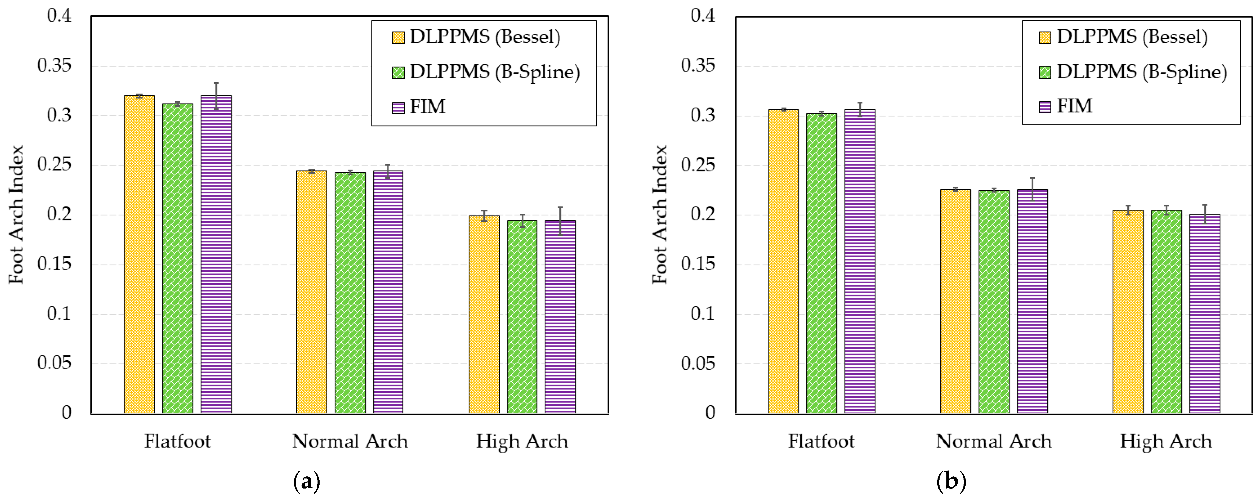
To facilitate comparison of bilateral FAI differences across foot arch types, bar charts display the left and right foot FAI measurements obtained from three distinct methods: DLPPMS with Bessel interpolation, DLPPMS with B-spline interpolation, and the conventional FIM method, as illustrated in Figure 12. These visualizations serve as a complement to Table 1, Table 2 and Table 3 by emphasizing the differences in FAI values associated with each method across flatfoot, normal arch, and high arch conditions. The error bars in Figure 12 represent the standard deviation (SD) calculated from 10 repeated measurements, providing an indication of the measurement consistency for each approach.

The measurement results demonstrate a high level of agreement between the FAI values obtained using the DLPPMS and those derived from the FIM method, suggesting that the DLPPMS serves as a reliable and objective alternative to conventional footprint-based assessments. In contrast, the FIM method demonstrated greater variability across repeated measurements.

To assess the measurement stability of each method, statistical metrics including the SD, coefficient of variation (CV), and mean absolute deviation (MAD) were calculated to quantify variability. The results of this analysis are summarized in

Table 4. Statistical analysis of foot arch index (FAI) variability for the flatfoot group.

Statistical Analysis	DLPPMS (Bessel)		DLPPMS (B-Spline)		FIM
	Left Foot	Right Foot	Left Foot	Left Foot	Right Foot	Left Foot
CV	0.0049	0.0045	0.0074	0.0049	0.0045	0.0074
SD	0.0016	0.0014	0.0023	0.0016	0.0014	0.0023
MAD	0.0013	0.0012	0.0020	0.0013	0.0012	0.0020

,

Table 5. Statistical analysis of foot arch index (FAI) variability for the normal arch group.

Statistical Analysis	DLPPMS (Bessel)		DLPPMS (B-Spline)		FIM
	Left Foot	Right Foot	Left Foot	Left Foot	Right Foot	Left Foot
CV	0.0056	0.0057	0.0080	0.0056	0.0057	0.0080
SD	0.0014	0.0013	0.0019	0.0014	0.0013	0.0019
MAD	0.0012	0.0011	0.0018	0.0012	0.0011	0.0018

and

Table 6. Statistical analysis of foot arch index (FAI) variability for the high arch group.

Statistical Analysis	DLPPMS (Bessel)		DLPPMS (B-Spline)		FIM
	Left Foot	Right Foot	Left Foot	Left Foot	Right Foot	Left Foot
CV	0.0267	0.0218	0.0310	0.0267	0.0218	0.0310
SD	0.0053	0.0045	0.0060	0.0053	0.0045	0.0060
MAD	0.0044	0.0034	0.0051	0.0044	0.0034	0.0051

.

The DLPPMS with Bessel interpolation exhibited the highest measurement stability for the flatfoot group, as shown in Table 4. For the right foot, the CV, SD, and MAD were 0.0045, 0.0014, and 0.0012, respectively; for the left foot, the corresponding values were 0.0049, 0.0016, and 0.0013, indicating excellent consistency across repeated measurements. By contrast, the FIM method showed the greatest variability, with CV, SD, and MAD values of 0.0232, 0.0062, and 0.0062 for the right foot, and 0.0408, 0.0131, and 0.0115 for the left foot, reflecting lower operational stability and greater susceptibility to manual segmentation errors. The DLPPMS with B-spline interpolation demonstrated moderate performance, with CV, SD, and MAD values of 0.0068, 0.0023, and 0.0017 for the right foot, and 0.0074, 0.0026, and 0.0020 for the left foot, suggesting reasonable but less optimal measurement consistency compared to the Bessel-based approach.

The DLPPMS with Bessel interpolation again demonstrated the highest measurement stability for the normal arch group, as shown in Table 5. For the right foot, the CV, SD, and MAD were 0.0032, 0.0010, and 0.0009, respectively; for the left foot, the corresponding values were 0.0056, 0.0016, and 0.0012, confirming the robustness and repeatability of the Bessel-based approach. The DLPPMS with B-spline interpolation showed slightly greater variability, with CV, SD, and MAD values of 0.0080, 0.0023, and 0.0016 for the right foot, and 0.0080, 0.0023, and 0.0018 for the left foot, indicating moderate consistency. The FIM method exhibited the highest variability, with CV, SD, and MAD values of 0.0522, 0.0118, and 0.0104 for the right foot, and 0.0277, 0.0066, and 0.0062 for the left foot, reflecting lower stability and greater susceptibility to manual processing errors.

The FIM method once again exhibited the highest measurement variability for the high arch group, as shown in Table 6. For the right foot, the CV, SD, and MAD were 0.0404, 0.0079, and 0.0079, respectively; for the left foot, the corresponding values increased to 0.0713, 0.0094, and 0.0117, indicating poor repeatability and reduced reliability in manually segmented measurements. In comparison, the DLPPMS with Bessel interpolation maintained better consistency, with CV, SD, and MAD values of 0.0218, 0.0041, and 0.0034 for the right foot, and 0.0267, 0.0052, and 0.0044 for the left foot. The DLPPMS with B-spline interpolation showed moderate variability, with values of 0.0232, 0.0040, and 0.0041 for the right foot, and 0.0310, 0.0051, and 0.0051 for the left foot. A slightly elevated fluctuation was observed on the right foot, indicating a marginal reduction in stability compared to the Bessel-based approach.

In summary, the results demonstrate that all three methods, including the DLPPMS with Bessel interpolation, the DLPPMS with B-spline interpolation, and the conventional FIM method, are capable of producing consistent FAI measurements. However, the DLPPMS shows clear advantages in terms of measurement stability and precision. Among the interpolation techniques, Bessel interpolation provides smoother plantar pressure maps and lower variability, making the DLPPMS especially suitable for applications that require high repeatability and diagnostic reliability, such as clinical assessments. In comparison, the lower accuracy of the FIM method is primarily due to its reliance on manual processing. The need to manually outline and align the plantar region introduces human-induced variability, which reduces the precision and consistency of the resulting FAI values.

5. Conclusions

This study developed a deep learning-based plantar pressure measurement system (DLPPMS) to improve the precision and repeatability of foot arch index (FAI) estimation under static conditions. The system integrates YOLOv11n-pose for anatomical keypoint detection, YOLOv11n-seg for plantar region segmentation, and numerical algorithms including Bessel and B-spline interpolation. With this framework, the system achieved automated identification of critical landmarks such as the heel and the base of the second toe, with a root mean square error (RMSE) of 3.8 mm in keypoint localization. The segmentation module effectively excluded the toe regions to retain only the load-bearing plantar surface, achieving an average precision of 0.99 at an IoU threshold of 0.50 and 0.98 across the 0.50–0.95 range. Compared with the conventional footprint imaging measurement method, the DLPPMS demonstrated strong agreement across flatfoot, normal arch, and high arch feet, with average FAI deviations below 0.01. Among the interpolation methods, Bessel interpolation exhibited the highest stability, producing smoother and anatomically coherent pressure maps while overcoming the challenge of limited sensor resolution. Collectively, these results highlight the DLPPMS as a reliable, accurate, repeatable, and real-time tool for static foot posture evaluation. Beyond its technical contributions, the DLPPMS provides significant clinical value as a low-cost, standardized, and rapid method for foot arch assessment, offering clinicians immediate support for screening, patient monitoring, rehabilitation follow-up, and decision-making in clinical practice. Nevertheless, this study has certain limitations, including the limited number of sensing points, the small sample size, and the absence of large-scale clinical validation. The relatively small sample size reflects the methodological validation nature of this work rather than large-scale clinical trials. These aspects will be addressed in future work to further strengthen the clinical applicability and generalizability of the system.

Future work will, therefore, focus on extending the system from static measurement to dynamic gait analysis, enabling more comprehensive evaluation of foot function during walking. Validation with larger and more diverse populations will also be pursued, together with the integration of additional sensing modalities to enrich diagnostic insights. These developments are expected to further expand the applicability of the DLPPMS and enhance its impact on clinical diagnostics, preventive healthcare, sports science, and rehabilitation monitoring.