Diffusion-Q Synergy (DQS): A Generative Approach to Policy Optimization via Denoised Action Spaces

Abstract

In this paper, we propose a novel algorithm that integrates diffusion models with reinforcement learning, called Diffusion-Q Synergy (DQS). The methodology formalizes an equivalence relationship between the iterative denoising process in diffusion models and the policy improvement mechanism in Markov Decision Processes. Central to this framework is a dual-learning mechanism: (1) a parametric Q-function is trained to evaluate noise prediction trajectories through temporal difference learning, effectively serving as a differentiable critic for action quality assessment; and (2) this learned Q-scoring function is then structurally integrated into the training objective of a conditional diffusion model, formulating a constrained optimization problem that simultaneously maximizes expected returns while minimizing policy deviation from behavioral priors. The algorithmic superiority of DQS stems from its hybrid architecture combining the (i) diffusion policy cloning for stable behavior regularization and (ii) adaptive noise rectification through Q-value-guided key denoising step correction, which is particularly effective for refining suboptimal action sequences, thereby guiding the entire diffusion trajectory toward policy optimality. Rigorous ablation studies across benchmark environments demonstrate statistically significant performance improvements ($p<0.01$) over baseline methods in both computational efficiency and asymptotic policy quality. The implementation has been open-sourced at AOLIGOOD/Diffusion_Q_Synergy, to facilitate reproducibility.

1. Introduction

Contemporary industrial systems have experienced unprecedented expansion and development, with control objects evolving toward higher-dimensional, increasingly nonlinear, and more complex operational objectives. This paradigm shift has imposed substantially elevated demands on control system design. Reinforcement learning (RL) has emerged as a particularly promising solution, as it obviates the need for complete a priori knowledge of environmental dynamics. This capability enables robotic systems, automated equipment, and other intelligent agents to autonomously adapt and optimize their behavior in dynamic, uncertain environments, thereby enhancing operational efficiency, minimizing resource expenditure, and facilitating more sophisticated task execution. Notably, in domains such as Large Language Models (LLMs), embodied intelligence, and autonomous driving, RL has proven instrumental in developing more flexible and responsive solutions that drive technological innovation.

The conceptual foundations of RL can be traced back to the mid-20th century, when Minsky [1] first formalized the notions of “reinforcement” and “reinforcement learning”. His seminal work emphasized the critical role of reward–punishment mechanisms in learning processes and identified trial-and-error as the fundamental paradigm of RL.

From a methodological perspective, dynamic programming provided essential mathematical tools for RL development. Bellman’s 1960 formulation of dynamic programming [2,3] not only established the theoretical framework for solving Markov Decision Processes (MDPs) but also introduced the Bellman equation, which remains the cornerstone of modern RL algorithms. Subsequent work on policy iteration methods further refined the MDP solution framework. However, these early developments remained largely theoretical until the breakthrough introduction of Q-learning [4]. This algorithm enabled practical applications by discovering optimal action policies without requiring explicit reward functions or state transition models. As a model-free approach that provably converges to optimal policies in deterministic MDP, Q-learning represented a watershed moment in RL research.

The 21st century witnessed transformative advances with the integration of deep learning. In 2013, DeepMind’s pioneering work [5] combined deep neural networks with Q-learning to create Deep Q-Networks (DQNs), effectively addressing the critical challenge of high-dimensional state space representation. This innovation spawned numerous advanced algorithms, including DDQN [6], TRPO [7], PPO [8], DDPG [9], A3C [10], SAC [11], TD3 [12], and [13,14,15], collectively propelling RL into mainstream artificial intelligence research and applications.

While deep neural networks have significantly enhanced the capability of reinforcement learning agents to handle complex decision-making tasks, conventional RL methodologies necessitate continuous environmental interaction for experience collection during agent training. This exploration process often incurs substantial costs in real-world applications. Specifically, agents typically require millions of interactions to develop effective policies, which proves particularly problematic in domains such as robotic control and autonomous driving—scenarios where such extensive interaction is not only cost-prohibitive but also poses significant safety risks. Furthermore, the inherent randomness in environmental interactions coupled with frequent policy updates during exploration may lead to training gradient instability.

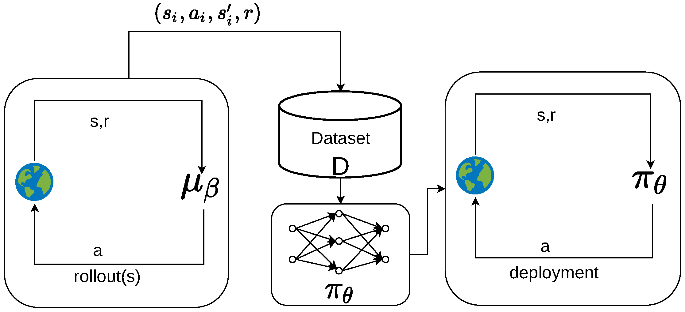
Offline reinforcement learning (Figure 1), also known as batch reinforcement learning, has emerged as a promising research direction to address these challenges. This paradigm enables policy learning exclusively from pre-collected datasets, eliminating the need for online environmental interaction. The principal advantages of this approach are threefold: First, the use of fixed datasets substantially improves training stability; second, the elimination of real-time interaction allows for the optimal utilization of historical data, particularly valuable in high-cost or safety-critical applications (e.g., healthcare, autonomous vehicles, and robotics); finally, offline RL facilitates policy optimization using large-scale offline datasets, thereby mitigating traditional RL’s sample inefficiency while enhancing data utilization.

However, offline RL introduces unique challenges. Since it relies solely on pre-collected data, standard RL methods encounter distributional shift during policy optimization, generating out-of-distribution actions. Q-learning exacerbates this issue through extrapolation error, overestimating the value of OOD (out-of-distribution actions). This overestimation triggers a destructive feedback loop: the policy increasingly selects overestimated OOD actions, and the Q-function amplifies these errors, ultimately resulting in significant policy performance degradation.

Prior research in offline RL has typically addressed this problem through one of four approaches: 1. Policy Constraints [12,16,17,18,19,20]: Restricting the policy from selecting actions that deviate substantially from the offline data distribution. While effective in preventing OOD action selection and subsequent Q-value overestimation, this method renders policy learning critically dependent on dataset quality. 2. Uncertainty Estimation [21,22]: Adjusting policies based on estimated uncertainty (e.g., in policy or value functions) to avoid decisions in high-uncertainty regions. Practical implementations often underestimate uncertainty, potentially increasing OOD action selection. 3. Regularization [19,23,24]: Incorporating regularization terms without explicit policy constraints. Generally less conservative than policy constraints, this approach typically achieves superior performance in practice. 4. Trajectory Optimization [25,26]: Framing RL as a sequence generation task with multiple state–action anchor points throughout trajectories. While theoretically eliminating distributional shift, this method demands substantial computational resources and exhibits slow prediction times.

In the majority of prior work, the policy is typically parameterized as a Gaussian distribution, with its mean and (often diagonal) covariance determined by the output of a neural network. However, in the context of offline reinforcement learning, datasets are frequently collected from a mixture of diverse behavior policies. Consequently, the true underlying behavior policy may exhibit complex characteristics such as strong multimodality, significant skewness, or intricate dependencies between different action dimensions. A standard diagonal Gaussian policy inherently struggles to adequately model these complex properties [27]. This inherent limitation in policy representation capacity can severely constrain the expressiveness of the learned policy. As a result, offline reinforcement learning methods that rely on this restrictive parameterization, particularly those incorporating policy regularization, often tend to converge to suboptimal policies and may exhibit performance that is slightly inferior compared to alternative approaches.

Owing to the superior performance of diffusion models, recent studies have increasingly adopted them as policy networks, as exemplified by Diffuser [28] and Diffusion Policy [29]. However, these methods rely solely on behavioral cloning for policy training without directly optimizing the policy, leading to performance that critically depends on the neural network’s scale and often suffers from suboptimal real-time efficiency. In contrast, Diffusion-QL aligns with our approach by leveraging the Q-function for policy improvement to learn the optimal policy. Nevertheless, its training process necessitates frequent sampling, which substantially increases computational overhead. Notably, if we model the action distribution of the dataset as a perturbed optimal policy distribution, based on prior studies [30], the later stages of the denoising process have the most significant impact on sample quality, where the noise prediction near $t=0$ can be viewed as estimating the perturbed noise of the optimal policy distribution. This insight enables highly efficient sampling during training with only a minimal number of diffusion steps.

Building upon these observations, we propose DQS, a novel reinforcement learning algorithm that formalizes the dataset’s action distribution as a noise-injected optimal policy distribution and employs a diffusion (or score-based) model for policy regularization. Specifically, DQS utilizes a multilayer perceptron (MLP)-based Denoising Diffusion Probabilistic Model (DDPM) as its policy. The training objective comprises two key components: 1. a behavioral cloning term, ensuring alignment with the empirical action distribution of the training data, and 2. a policy optimization term, where the Q-function guides the diffusion model in noise prediction during the later stages of denoising. Crucially, this framework enables highly efficient training by requiring only minimal denoising steps during sampling.

In summary, this paper contributes DQS, an improved offline RL algorithm that leverages diffusion models’ exceptional data distribution learning capability for precise policy regularization while successfully employing Q-learning to guide noise prediction in suboptimal actions toward optimal action discovery. Comprehensive evaluation on the D4RL offline RL benchmark demonstrates that DQS achieves performance comparable to or superior to recent offline RL baselines.

2. Preliminaries

This section systematically delineates the formal definition of Markov Decision Processes, the application of weighted regression to policy improvement, and the mathematical underpinnings of diffusion models. This exposition establishes the theoretical foundation for the subsequent development of methodologies.

2.1. Offline Reinforcement Learning

A Markov Decision Process (MDP) is formally defined as a tuple $\mathcal{M}=(\mathcal{S},\mathcal{A},P,R,\gamma )$. $\mathcal{S}$ represents the state space, consisting of the set of all possible states. $\mathcal{A}$ represents the action space, consisting of the set of all possible actions. $P\left(s^{\prime }\right|s,a)$ is the state transition probability function, which specifies the probability of transitioning to state $s^{\prime }$ from state s when taking action a. This function satisfies the property ${\sum }_{s^{\prime }}P\left(s^{\prime }\right|s,a)=1$ for all $s\in \mathcal{S},a\in \mathcal{A}$. $R(s,a)$ is the reward function, which defines the immediate reward received upon taking action a in state s. $\gamma \in [0,1)$ is the discount factor, which weights the importance of immediate versus future rewards.

Markov Decision Processes constitute the theoretical foundation for reinforcement learning, providing a mathematical framework to model the interaction dynamics between an intelligent agent and its environment. The primary objective in reinforcement learning is to learn an optimal policy ${\pi }_{\theta }$ by maximizing the expected cumulative discounted return, denoted by $J\left({\pi }_{\theta }\right)$:

$$\begin{array}{c}\hfill J\left({\pi }_{\theta }\right)=E_{\tau \sim {\pi }_{\theta }}\left[\sum _{t=0}^{\infty }{\gamma }^{t}R(s_t,a_t)\right]\end{array}$$

(1)

Here, $\tau =(s_0,a_0,s_1,a_1,\dots )$ denotes a trajectory (or sequence of state–action pairs) generated by following policy ${\pi }_{\theta }$.

Specifically, the action–value function $Q^{{\pi }_{\theta }}(s,a)$ is defined as the expected cumulative discounted return obtained by taking action a in state s and thereafter following policy ${\pi }_{\theta }$:

$$\begin{array}{c}\hfill Q^{{\pi }_{\theta }}(s_t,a_t)=E_{a\sim {\pi }_{\theta }}\left[G_t|s_t=s,a_t=a\right]\end{array}$$

(2)

where $G_t={\sum }_{k=t}^{\infty }{\gamma }^{k-t}R(s_k,a_k)$ is the cumulative discounted return from timestep t.

The action–value function $Q^{{\pi }_{\theta }}$ satisfies the Bellman equation, which offers a recursive relationship between the value of a state–action pair and the expected value of the subsequent state–action pair:

$$\begin{array}{c}\hfill Q^{{\pi }_{\theta }}(s_t,a_t)=R(s_t,a_t)+\gamma E_{s_{t+1}\sim P,a_{t+1}\sim {\pi }_{\theta }}\left[Q^{{\pi }_{\theta }}(s_{t+1},a_{t+1})|s_t,a_t\right]\end{array}$$

(3)

Maximizing the reinforcement learning objective function is equivalent to maximizing the expected values of the action–value function.

In contrast to online reinforcement learning, offline reinforcement learning solely utilizes a static dataset $\mathbb{D}=\left\{(s_i,a_i,r_i,s_i^{\prime })\right\}$ of previously collected transitions for policy optimization, without explicit interaction with the environment. This dependency introduces significant challenges, including distribution shift (or covariate shift) and extrapolation errors, as the learned policy might select actions outside the distribution of the dataset’s behavior policy $\mu$. To address these challenges, a common approach in offline RL is to constrain the learned policy $\pi$ to adhere closely to the behavior policy $\mu$ that generated the dataset $\mathbb{D}$, while concurrently optimizing for high Q-values.

This objective is formally expressed as maximizing the expected Q-value under the behavior policy’s state distribution ${\rho }_{\mu }\left(s\right)$, penalized by the KL divergence between the learned policy $\pi (·|s)$ and the behavior policy $\mu (·|s)$:

$$\begin{array}{cc}\hfill arg\underset{\pi }{max}& {\int }_S{\rho }_{\mu }\left(s\right){\int }_A\pi \left(a\right|s)Q_{\varphi }(s,a)dads\hfill \\ \hfill & -{\displaystyle \frac{1}{\alpha }}{\int }_S{\rho }_{\mu }\left(s\right)D_{\mathrm{KL}}(\pi (·|s)\parallel \mu (·|s))ds.\hfill \end{array}$$

(4)

Here, $Q_{\varphi }(s,a)$ denotes the learned action–value function parameterized by $\varphi$, ${\rho }_{\mu }\left(s\right)$ is the stationary state distribution induced by the behavior policy $\mu$, and $D_{\mathrm{KL}}$ represents the Kullback-Leibler divergence. The term $-{\displaystyle \frac{1}{\alpha }}{D}_{\mathrm{KL}}(\pi (·|s)\parallel \mu (·|s))$ acts as a regularization term, scaled by ${\displaystyle \frac{1}{\alpha }}$ (where $\alpha$ is a hyperparameter) to penalize deviations of the learned policy $\pi$ from the behavior policy $\mu$.

2.2. Policy Improvement via Weighted Regression

The optimal policy ${\pi }^{*}$ for the objective in Equation (4) is derived using Lagrange multipliers, yielding [17]

$${\pi }^{*}\left(a\right|s)={\displaystyle \frac{1}{Z\left(s\right)}}\mu \left(a\right|s)exp\left(\alpha Q_{\varphi }(s,a)\right),$$

(5)

where $Z\left(s\right)$ is the partition function. This expression for ${\pi }^{*}$ represents a policy improvement step.

Directly sampling from ${\pi }^{*}$ requires explicit modeling of the behavior policy $\mu$. This poses a considerable challenge, particularly in continuous action spaces, as $\mu$ can be highly complex or multimodal. Previous methods [17] address this challenge through projecting the optimal policy ${\pi }^{*}$ onto a parameterized policy class ${\pi }_{\theta }$. This projection is typically accomplished by minimizing the KL divergence between ${\pi }^{*}$ and ${\pi }_{\theta }$:

$$\begin{array}{cc}\hfill & arg\underset{\theta }{min}{\mathbb{E}}_{s\sim D^{\mu }}\left[D_{\mathrm{KL}}\left({\pi }^{*}(·|s)\parallel {\pi }_{\theta }(·|s)\right)\right]\hfill \\ \hfill =& arg\underset{\theta }{max}{\mathbb{E}}_{(s,a)\sim D^{\mu }}\left[{\displaystyle \frac{1}{Z\left(s\right)}}log{\pi }_{\theta }\left(a\right|s)exp\left(\alpha Q_{\varphi }(s,a)\right)\right].\hfill \end{array}$$

(6)

This approach is typically referred to as weighted regression or advantage-weighted regression (specifically when Q is replaced by the advantage $A=Q-V$), where $exp\left(\alpha Q_{\varphi }(s,a)\right)$ serves as the regression weight.

2.3. Diffusion Models

Diffusion models [31,32] represent a prominent class of generative models in deep learning, which employ thermodynamic diffusion principles to iteratively reconstruct data from noise. These models have exhibited notable performance in various generation tasks, including image, audio, and video synthesis. The framework encompasses two fundamental phases: the forward process and the reverse process.

Forward Process: The forward process, also known as the diffusion phase, systematically transforms the original data sample $x_0$ into pure Gaussian noise through T discrete timesteps. This transformation is mathematically represented as

$$\begin{array}{c}\hfill x_t={\alpha }_t{x}_{t-1}+{\beta }_tϵ,ϵ\sim \mathcal{N}(0,I)\end{array}$$

(7)

Here, ${\beta }_t$ denotes the noise intensity at step t, $ϵ\sim \mathcal{N}(0,I)$ represents standard normal distribution noise, and ${\alpha }_t$ corresponds to the scaling factor at timestep t.

Reverse Process: The reverse process constitutes the central innovation of diffusion models, which aims to learn the gradual reconstruction of data $x_0$ from noisy observations $x_t$. This parameterized Markov chain is realized through neural network learning, with the transition given by

$$\begin{array}{c}\hfill x_{t-1}={\displaystyle \frac{x_t-{\beta }_t{ϵ}_{\theta }(s_t,x_t,t)}{{\alpha }_t}}+{\sigma }_{t}z,z\sim \mathcal{N}(0,I)\end{array}$$

(8)

In this formulation, ${ϵ}_{\theta }(s_t,x_t,t)$ denotes the parameterized noise prediction network, while ${\sigma }_t$ represents the noise variance.

The neural network training objective is expressed as

$$\begin{array}{c}\hfill L_{DDPM}\left(\theta \right)=\mathbb{E}\left[\left|\right|ϵ(x_0,t)-{ϵ}_{\theta }(x_t,c,t){\left|\right|}^2\right]\end{array}$$

(9)

3. Diffusion-Q Synergy

As the control requirements of intelligent systems exhibit increasing complexity (e.g., dynamic gait regulation in quadrupedal robots, multimodal decision-making in autonomous vehicles), the limitations inherent in conventional control methodologies when applied to high-dimensional, nonlinear, and time-varying systems have become more pronounced. To effectively address these challenges, a novel offline reinforcement learning algorithm, predicated upon the diffusion model and designated as DQS, is proposed.

This methodology capitalizes on the progressive distribution-fitting capabilities characteristic of diffusion models to execute behavioral cloning based on the policy present within the dataset. Furthermore, through rigorous theoretical analysis, the mathematical equivalence between the reverse denoising process of the diffusion model and the policy learning process is demonstrably established. This equivalence ensures that the learned policy, denoted as ${\pi }_{\theta }$, maintains alignment with the dataset’s behavioral policy while simultaneously enabling the Q-learning-guided noise prediction network, ${ϵ}_{\theta }$, to generate optimized denoised actions.

3.1. Diffusion Policy Cloning

For the purpose of clearly distinguishing between two distinct temporal processes, the following notation is adopted: Specifically, the subscript $t\in \{1\dots T\}$ is utilized to denote discrete timesteps associated with the diffusion process. The superscript $n\in \{1\dots N\}$ is employed to represent timesteps within the reinforcement learning (RL) trajectory.

In the field of reinforcement learning (RL), a policy $\pi$ is formally defined as a conditional probability function that characterizes the probability distribution over actions given a specific state. Concurrently, diffusion models, as a class of generative models, can also be conceptualized as a conditional probability function. This function describes the probabilistic generation of a final output $x_0$ (e.g., an action a) from an initial random noise $x_T$, contingent upon a given state s, through an iterative reverse denoising process. Given the demonstrated efficacy of diffusion models in accurately modeling and generating complex data distributions, it is posited that these models can be directly employed for the parameterization of policies within RL frameworks.

$$\begin{array}{c}\hfill {\pi }_{\theta }\left(a\right|s)=P_{\theta }\left(x_0\right|s,x_T)\end{array}$$

(10)

In this context, ${\pi }_{\theta }\left(a\right|s)$ represents the learned policy, and $P_{\theta }\left(x_0\right|s,x_T)$ represents the reverse process of the diffusion model, indicating the likelihood of the diffusion model generating a clean sample $x_0$ given the state s and the final noisy sample $x_t$.

A rigorous mathematical equivalence is established between the conditional generation process of the diffusion model and the process of RL policy optimization. Consequently, the standard objective function utilized in reinforcement learning may be reformulated as follows:

$$\begin{array}{cc}\hfill J\left(\theta \right)& ={\mathbf{E}}_{s\sim \mathcal{D},a\sim {\pi }_{\theta }(·|s)}\left[\sum _{t=0}^{\infty }{\gamma }^{t}R(s,a)\right]\hfill \\ \hfill & =\mathbf{E}\left[{\mathcal{D}}_{KL}\left({\pi }^{\star }\left(a\right|s)\Vert P_{\theta }\left(x_0\right|s,x_T,T)\right)\right]\hfill \\ \hfill & =\mathbf{E}\left[{\mathcal{D}}_{KL}\left({\pi }^{\star }\left(a\right|s)\Vert {\pi }_{\theta }\left(a\right|s)\right)\right]\hfill \end{array}$$

(11)

Here, $\theta$ represents the set of learnable parameters, and ${\pi }^{\star }\left(a\right|s)$ denotes the optimal policy.

Remark 1. 

${\pi }^{\star }$ is defined as the policy that maximizes $J\left(\theta \right)$:

$$\begin{array}{c}\hfill {\pi }^{\star }=argmaxJ\left(\pi \right)\end{array}$$

(12)

If ${\pi }^{\star }$ matches ${\pi }_{\theta }$, i.e., ${\pi }^{\star }={\pi }_{\theta }$, then $J\left(\theta \right)$ must reach its maximum value. Therefore, minimizing the discrepancy between ${\pi }_{\theta }$ and ${\pi }^{\star }$ can be regarded as a surrogate objective for maximizing $J\left(\theta \right)$, as expressed in Equation (12).

Remark 2. 

Within the framework presented in Equation (10), the policy improvement process characteristic of reinforcement learning is modeled as the reverse denoising trajectory of the diffusion model, wherein a clean sample $x_0$ is generated from noise ϵ. This specific formulation necessitates two conditions: 1. The diffusion model must possess the requisite capacity to approximate arbitrary policy distributions, a capability previously demonstrated in ref. [33]. 2. Knowledge or reliable estimability of the optimal policy ${\pi }^{\star }$ is required. It is pertinent to note that in the context of offline RL, ${\pi }^{\star }$ is typically unknown and must therefore be inferred from a dataset that has been generated by a suboptimal behavioral policy, denoted by μ.

To apply ${\mathcal{D}}_{KL}$ definition to the objective function,

$$\begin{array}{c}\hfill J\left(\theta \right)={\mathbb{E}}_{s\sim {\rho }_{\mu }\left(s\right)}\left[{\mathbb{E}}_{a\sim {\pi }^{*}(·|s)}\left[log{\pi }^{*}\left(a\right|s)-log{P}_{\theta }\left(x_0\right|s,x_T)\right]\right]\end{array}$$

(13)

Following the methodology established in [31], the diffusion model’s training objective (Equation (9)) relates to the noise prediction error:

$$\begin{array}{c}\hfill -log{P}_{\theta }\left(x_0\right|s,x_T)\propto \sum _{t=1}^T{\mathbb{E}}_{ϵ\sim N(0,I)}\left[\left|\right|ϵ-{ϵ}_{\theta }(s,x_t,t){\left|\right|}^2\right].\end{array}$$

(14)

Thus, minimizing $J\left(\theta \right)$ is equivalent to minimizing the diffusion model’s noise prediction error.

3.2. Q-Learning-Guided Noise Prediction

Remark 3. 

Q-Learning-guided can be reformulated through the application of KL divergence to quantify the dissimilarity between the optimal policy ${\pi }^{\star }$ and the denoised action distribution $P_{\theta }\left(x_0\right|a_D,s)$ for a given state, thereby facilitating the guidance of noise prediction for suboptimal actions. However, analogous to the challenge encountered in Equation (12), the optimal policy remains unknown, necessitating the determination of its relationship with other components. As delineated in the preliminaries (Equation (5)), connections have been established between the behavioral policy μ and the optimal policy ${\pi }^{\star }$, as well as between the parameterized policy and ${\pi }^{\star }$. Correspondingly, a relationship between the denoising model ${ϵ}_{\theta }$ and the optimal policy can be derived.

Building upon the weighted regression formulation presented in Equation (6), it is further derived that

$$\begin{array}{c}\hfill {\pi }^{\star }(·|s)\propto P_{\theta }\left(x_0\right|a_D,s)·exp\left(\alpha Q(s,x_0)\right)\end{array}$$

(15)

In the context of offline reinforcement learning, weighted regression imposes a constraint on the policy to maintain proximity to $\mu$ while employing the Q-value as regression weights to direct policy optimization. Similarly, Q-Learning-guided term within the objective function adjusts the direction of noise prediction while preserving the overall noise prediction trajectory (a characteristic ensured by the behavior cloning term), thereby optimizing the policy to better approximate the optimal policy. Consequently, $J\left(\theta \right)$ is simplified by adapting the weighted regression methodology:

$$\begin{array}{c}\hfill J\left(\theta \right)={\mathbb{E}}_{s\sim {\rho }_{\mu }\left(s\right)}\left[{\mathbb{E}}_{a\sim {\pi }^{*}(·|s)}\left[log(\mu (·|s)+\alpha {\mathbb{E}}_{a\sim \mu (·|s)}\left[Q(s,a)\right]-log{P}_{\theta }\left(x_0\right|s,x_T)\right]\right].\end{array}$$

(16)

where $\alpha$ functions as a normalization factor for the Q-function.

Substituting Equation (14) into the $J\left(\theta \right)$ objective gives

$$\begin{array}{c}\hfill J\left(\theta \right)={\mathbb{E}}_{s\sim {\rho }_{\mu }\left(s\right)}\left[\sum _{t=1}^T{\mathbb{E}}_{ϵ\sim N(0,I)}\left[\left|\right|ϵ-{ϵ}_{\theta }(s,x_t,t){\left|\right|}^2\right]+\alpha {\mathbb{E}}_{a\sim \mu (·|s)}\left[Q(s,a)\right]\right].\end{array}$$

(17)

As indicated in Equation (17), the objective $J\left(\theta \right)$ is ultimately reduced to the evaluation of generated actions $x_0$ through the Q-network $Q_{\varphi }$. This process facilitates the adjustment of the diffusion model’s parameters $\theta$ to enable ${ϵ}_{\theta }$ to yield higher expected Q-values. Given that the objective $J\left(\theta \right)$ is defined by leveraging the Q-function, the accuracy of Q-value estimation is rendered critical. To mitigate potential overestimation issues, double Q-learning is employed for Q-function estimation. Specifically, two Q-networks, $Q_{{\varphi }_1}$ and $Q_{{\varphi }_2}$, are utilized to independently estimate action values, and their parameters are updated by minimizing the discrepancy between their estimates. This approach serves to reduce Q-value variance and enhance the stability of policy optimization. Furthermore, target networks are implemented to stabilize the training procedure. These networks, updated through Exponential Moving Average (EMA), contribute to relative stability during training by serving as delayed-update replicas for the computation of Q-value targets. The objective function for Q-learning is formulated as

$$\begin{array}{c}\hfill L_Q\left(\varphi \right)={\mathbf{E}}_{(s,a)\sim \mathcal{D}}\left[{\left(r+\gamma \underset{i=1,2}{min}{Q}_{{\varphi }_i^{\prime }}(s^{\prime },a^{\prime })-Q_{{\varphi }_i}(s,a)\right)}^2\right]\end{array}$$

(18)

Reducing the function to its simplest form, the complete optimization objective is expressed as

$$\begin{array}{c}\hfill J\left(\theta \right)={(ϵ-{ϵ}_{\theta }(s,x_t,t))}^2+\alpha {\mathbf{E}}_{(s,a_D)\sim \mathcal{D},x_0\sim P_{\theta }(·|s,a_D)}\left[Q_{\varphi }(s,x_0)\right]\end{array}$$

(19)

This section presents the derivation of the policy optimization term as a formulation that maximizes the expected Q-value of denoised actions. This derivation is predicated upon weighted regression under the premise of an unknown optimal policy. Through the application of double Q-learning and target networks, the stability and accuracy of Q-value estimation are enhanced. The final optimization objective integrates both the noise prediction error and Q-function-guided policy optimization, thereby ensuring behavior cloning while simultaneously adjusting the direction of noise prediction to approximate the optimal policy.

3.3. Algorithm Details

To help readers better understand our algorithm process, we will introduce the main steps of our algorithm below [34]:

1.

Initialization Phase: Initially, the noise prediction network ${ϵ}_{\theta }$ and dual Q-learning networks $Q_{{\varphi }_1},Q_{{\varphi }_2}$ are constructed and initialized, along with their corresponding target networks $Q_{{\varphi }_1^{\prime }},Q_{{\varphi }_2^{\prime }}$ and ${ϵ}_{{\theta }^{\prime }}$. Subsequently, the offline dataset ${\mathcal{D}}_{\mu }$ is loaded to acquire state-action-next state-reward tuples ($s,a,s^{\prime },r$) for use as training samples.

2.

Critic Training Phase: During this phase, potential actions $a^{\prime }$ for subsequent states $s^{\prime }$ are generated. The target Q-values are computed using the Bellman equation and the target networks. The loss function (Equation (18)) is computed by minimizing the mean squared error between the current state–action Q-values predicted by $Q_{{\varphi }_1}$ and $Q_{{\varphi }_2}$ and their target values. The backpropagation process is then employed to update the parameters (${\varphi }_1$ and ${\varphi }_2$) of the dual Q-network, thereby enhancing value estimation accuracy.

3.

Policy Training Phase: The policy training procedure comprises two principal components:

(a)

Behavior Cloning Term: Starting from actions within the dataset $a_D$, intermediate noisy states ($x_t$) are generated through random timestep noising ($ϵ\sim \mathcal{N}(0,\mathbf{I})$). These states, along with the corresponding timestep (t), are input into the noise prediction network ${ϵ}_{\theta }$ to yield predicted noise (${ϵ}_{\theta }(s,x_t,t)$). The loss function is computed by minimizing the mean squared error between the actual noise ($ϵ$) and the predicted noise (${ϵ}_{\theta }(s,x_t,t)$) for the current state (s) and timestep (t).

(b)

Policy Improvement Term: Optimized actions ($x_0$) are generated through the denoising process, starting from noisy samples derived from dataset actions $a_D$. Policy gradient signals are constructed by evaluating the Q-function values ($Q_{\varphi }$) for state s and the optimized action $x_0$.

The compound loss function (Equation (19)) integrates these two components, with gradient descent utilized to update the parameters ($\theta$) of the noise prediction network.

4.

Target Network Update: An Exponential Moving Average (EMA) mechanism is employed to execute soft updates on the target network parameters (${\varphi }_1^{\prime }$, ${\varphi }_2^{\prime }$, and ${\theta }^{\prime }$). This gradual update strategy effectively stabilizes the training process by mitigating instability induced by high target value variance, thereby promoting steady improvement in model performance.

During both policy training and critic training, policy gradient clipping is applied to ensure training stability. The pseudocode and specific algorithm are shown in the following Algorithm 1.

Algorithm 1 DQS

Require:  Initialize the score-based model ${ϵ}_{\theta }$, training parameters ${\varphi }_1$ and ${\varphi }_2$ of the action  evaluation model $Q_{\varphi }$, training parameters ${\varphi }_1^{\prime }$ and ${\varphi }_2^{\prime }$ of the target action evaluation  model $Q_{{\varphi }^{\prime }}$,Loading the Dataset $D_{\mu }$.   1: for each gradient step do   2:    $(s,a_D,r,s^{\prime })\sim D_{\mu }$, $i\sim \mathrm{Uniform}(1,N)$, $ϵ\sim \mathcal{N}(0,\mathbf{I})$   3:    // Training Critic   4:    Sample $a^{*}$ by $a^{*}={\displaystyle \frac{x_t-\beta {ϵ}_{\theta }(s,x_t,t)}{\alpha }}$   5:    Update ${\varphi }_1$ and ${\varphi }_2$ by (18)   6:    // Training Policy   7:    Adding Noise to $a_D$ to get $a_n$   8:    Recovering $a^{*}$ by $a^{*}={\displaystyle \frac{a_n-\beta {ϵ}_{\theta }(s,x_t,t)}{\alpha }}\mathrm{for}t>n$   9:    Update $\theta$ by (19) 10:    // Update Target Network 11:    Update ${\varphi }_1^{\prime }$ and ${\varphi }_2^{\prime }$ by EMA 12:    Update ${\theta }^{\prime }$ by EMA 13: end for

4. Experimental Evaluation

The efficacy of the proposed methodology was systematically evaluated using the D4RL benchmark dataset [35], a widely recognized standard in offline reinforcement learning. To comprehensively validate the algorithm’s performance within the domain of intelligent control systems, the standard Gym test environments were selected as the evaluation platform. This test suite comprises three representative locomotion tasks: Hopper-v2, Walker2d-v2, and HalfCheetah-v2. Additionally, the Kitchen-v2 environment was included to assess the algorithm’s capability in complex manipulation tasks. Each task presents distinct challenges in biomechanical control, simulating various robotic locomotion and manipulation paradigms.

The Hopper-v2 environment models the control dynamics of a monopedal robotic system, analogous to the locomotion observed in kangaroos. This task requires the precise regulation of torque at the agent’s articulated joints to achieve stable forward hopping while concurrently maintaining dynamic equilibrium. The primary control objective is the joint optimization of forward velocity and postural stability to prevent instability or falls.

In the Walker2d-v2 environment, the control of a bipedal robotic system is simulated, emulating the mechanical principles of human ambulation. Effective control in this environment necessitates the coordinated application of torque across multiple leg joints to generate and sustain stable gait patterns. The central control challenge lies in the simultaneous maximization of forward velocity and preservation of upright balance.

The HalfCheetah-v2 environment simulates the control requirements of a quadrupedal robotic platform, inspired by the locomotion of cheetahs. Successful performance in this task demands sophisticated inter-limb coordination to achieve high-speed running gaits. The paramount control objective centers on maximizing horizontal velocity through the optimal distribution of torque across all actuated joints.

The Kitchen environment introduces a new dimension of evaluation by simulating a robotic manipulation scenario with multiple articulated objects. This environment tests the agent’s ability to perform sequential manipulation tasks, such as opening microwave doors, moving kettles, and turning knobs, requiring precise motor control and long-term task planning. The key challenge lies in coordinating high-dimensional continuous control while maintaining object interactions and avoiding collisions in a constrained workspace.

4.1. Comparison with Other Methods

Baselines

To establish a comprehensive performance benchmark, the proposed approach was systematically evaluated against several representative baselines from distinct methodological categories.

Within the domain of regularization-based offline reinforcement learning, baselines include Conservative Q-Learning (CQL) [23], TD3+BC [12], DQL [36], AWR [17], SAC [11], BEAR [37], BCQ [16], and Implicit Q-Learning (IQL) [19]. Within the model-based offline RL paradigm, Model-Based Offline Planning (MBOP) [38] was considered. Additionally, a comparative analysis was performed against trajectory prediction approaches, specifically Decision Transformer (DT) [25], Trajectory Transformer (TT) [26], and Diffuser [28].

The reported performance metrics for baseline methods are derived from either (1) the optimal results published in their respective original papers, or (2) the standardized evaluations conducted by ref. [35]. Our experimental results (see

Table 1. Comparing performance of DQS with other baseline algorithms.

Gym Tasks	BC	CQL	IQL	DT	TT	TD3+BC	Diffuser	MBOP	DQL	DQS (Ours)
Medium-Expert-HalfCheetah	55.2	91.6	86.7	86.8	95.0	90.7	88.9	105.9	96.8	94.0 ± 0.94
Medium-Expert-Hopper	52.5	105.4	91.5	107.6	110.0	98.0	103.3	55.1	111.1	97.0 ± 1.01
Medium-Expert-Walker2d	107.5	108.8	109.6	108.1	101.9	110.1	106.9	70.2	110.1	109.3 ± 0.29
Medium-HalfCheetah	42.6	44.0	47.4	42.6	46.9	48.3	42.8	44.6	51.1	47.0 ± 0.70
Medium-Hopper	52.9	58.5	66.3	67.6	61.1	59.3	74.3	48.8	90.5	84.6 ± 1.30
Medium-Walker2d	75.3	72.5	78.3	74.0	79.0	83.7	79.6	41.0	87.0	85.9 ± 1.70
Medium-Replay-HalfCheetah	36.6	45.5	44.2	36.6	41.9	44.6	37.7	42.3	47.8	44.4 ± 0.61
Medium-Replay-Hopper	18.1	95.0	94.7	82.7	91.5	60.9	93.6	12.4	101.3	96.1 ± 0.01
Medium-Replay-Walker2d	26.0	77.2	73.9	66.6	82.6	81.8	70.6	9.7	95.5	94.8 ± 1.32
Average	51.9	77.6	77.0	74.7	78.9	75.3	77.5	47.8	88.0	83.7
Kitchen Tasks	BC	CQL	IQL	BEAR	AWR	SAC	BCQ	BEAR-p	DQL	DQS (Ours)
Kitchen-Complete	33.8	43.8	62.5	0.0	0.0	15.0	8.1	0.0	84.0	72.1 ± 13.2
Kitchen-Partial	33.8	49.8	46.3	13.1	15.4	0.0	18.9	0.0	60.5	73.5 ± 6.6
Kitchen-Mixed	47.5	51.0	51.0	47.2	10.6	2.5	8.1	0.0	62.6	65.1 ± 13.5
Average	38.4	48.2	53.3	20.1	8.7	5.8	11.7	0.0	69.0	69.7

Only the absolute highest value in each row is highlighted in boldface. We report scores with 5 diffusion steps.

) were evaluated across five random seeds and 150 episodes, with performance variance quantified using standard deviation to ensure statistical reliability. This ensures a fair and consistent comparison framework. We employed permutation testing to assess statistical significance, with the detailed implementation and hyperparameters of our method provided in Appendix A,

Table A1. The hyperparameter settings for all evaluation tasks.

Task	$\mathit{\eta }$	$\mathit{\alpha }$	Grad Norm	Noise Scheduling
Medium-Expert-HalfCheetah	$3\times {10}^{-4}$	1.0	7.0	Cosine
Medium-Expert-Hopper	$3\times {10}^{-4}$	1.0	5.0	Cosine
Medium-Expert-Walker2d	$3\times {10}^{-4}$	1.0	5.0	Cosine
Medium-HalfCheetah	$3\times {10}^{-4}$	1.0	9.0	Cosine
Medium-Hopper	$3\times {10}^{-4}$	1.0	9.0	Cosine
Medium-Walker2d	$3\times {10}^{-4}$	1.0	1.0	Cosine
Medium-Replay-HalfCheetah	$3\times {10}^{-4}$	1.0	2.0	Cosine
Medium-Replay-Hopper	$3\times {10}^{-4}$	1.0	4.0	Cosine
Medium-Replay-Walker2d	$3\times {10}^{-4}$	1.0	4.0	Cosine
Kitchen-Complete	$3\times {10}^{-4}$	0.005	9.0	Cosine
Kitchen-Partial	$3\times {10}^{-4}$	0.005	10.0	Cosine
Kitchen-Mixed	$3\times {10}^{-4}$	0.005	10.0	Cosine

The hyperparameters for DQS in this table were adopted directly from the DQL baseline without additional tuning.

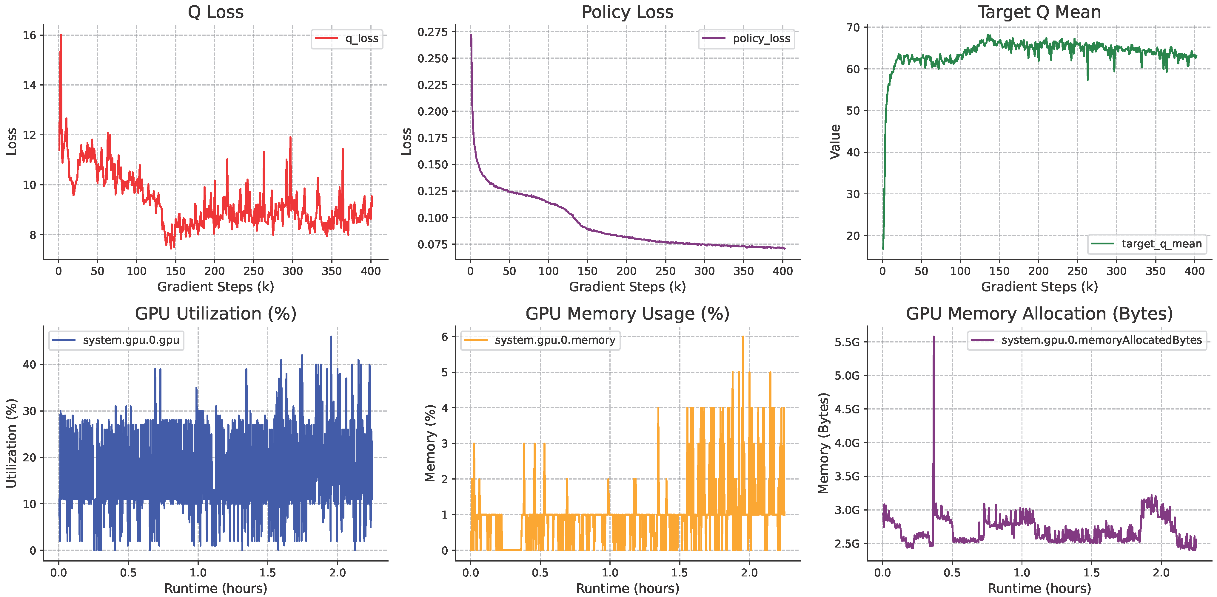
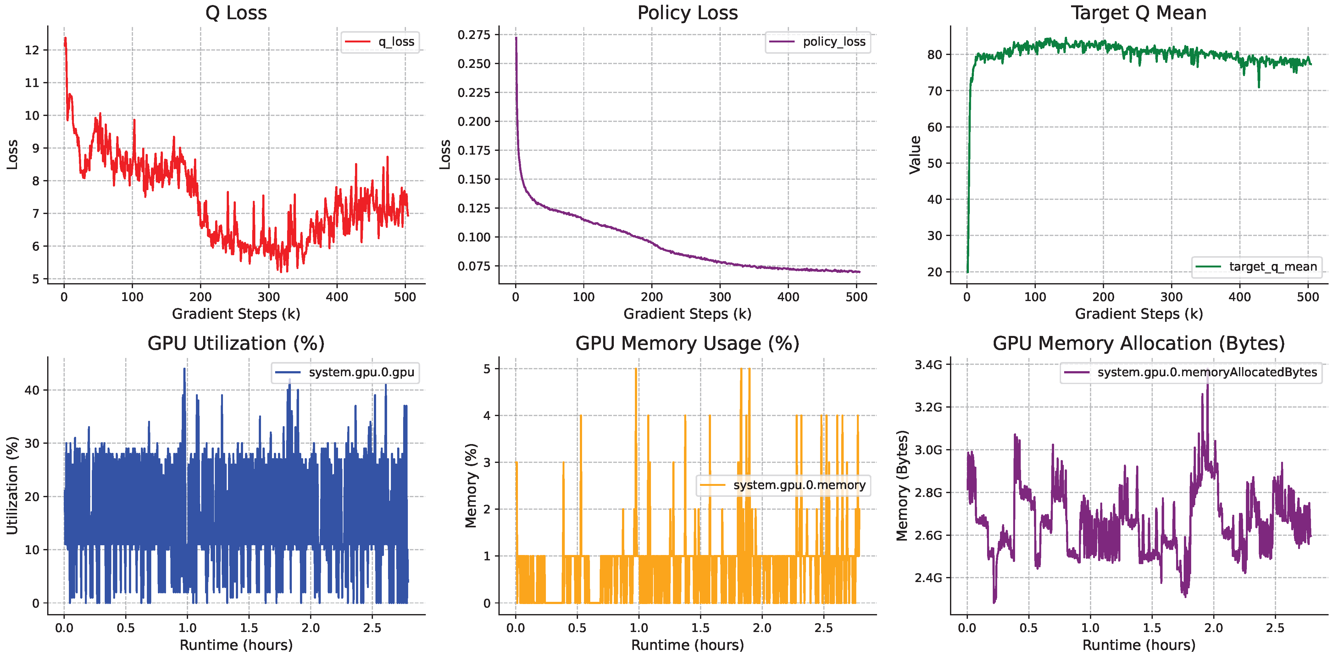
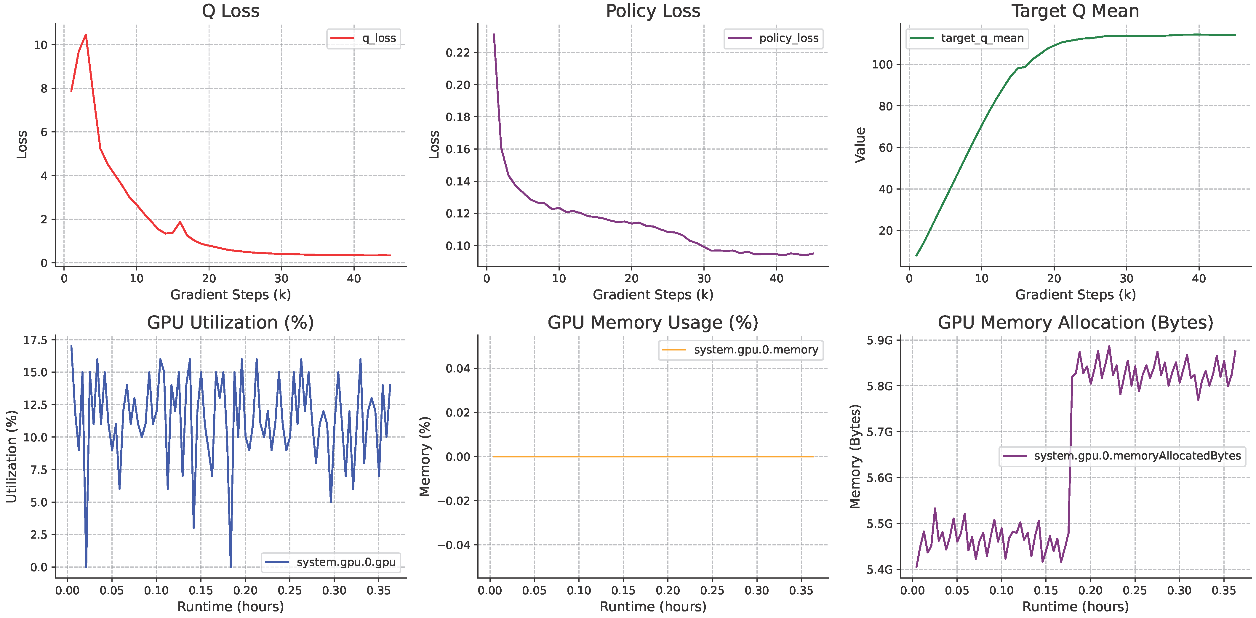
. Furthermore, the training details of our method are comprehensively described in Figure A1, Figure A2, Figure A3 and Figure A4.

Our method’s suboptimal performance in Gym tasks compared to DQL [36] might stem from the Q-function primarily guiding the denoising process only during its later stages. This late-stage guidance could be detrimental to effective motor control. Conversely, our method’s superior performance in Kitchen tasks could be attributed to the Q-function’s guidance during the earlier stages of the denoising process, which appears to be either less critical or even counterproductive for this specific task.

Table 2. Comparing computational efficiency of DQS with other baseline algorithms.

Time	CQL	BC	DT	TD3 + BC	DQL	DQS
Training Time	140 m	11 m	400 m	38 m	160 m	120 m
Inference Time	-	-	-	-	10.6 m	11.1 m

Training time is defined as the duration needed to accomplish one million training steps. Inference time is after 150 episodes of inference.

presents a comparison of the computational efficiency of an algorithm named DQS against several baseline algorithms on an NVIDIA 4090 GPU. The table shows two key metrics: training time and inference time. Training time is defined as the duration required to complete one million training steps. Inference time is measured after 150 inference episodes.

4.2. Impact of Hyperparameters

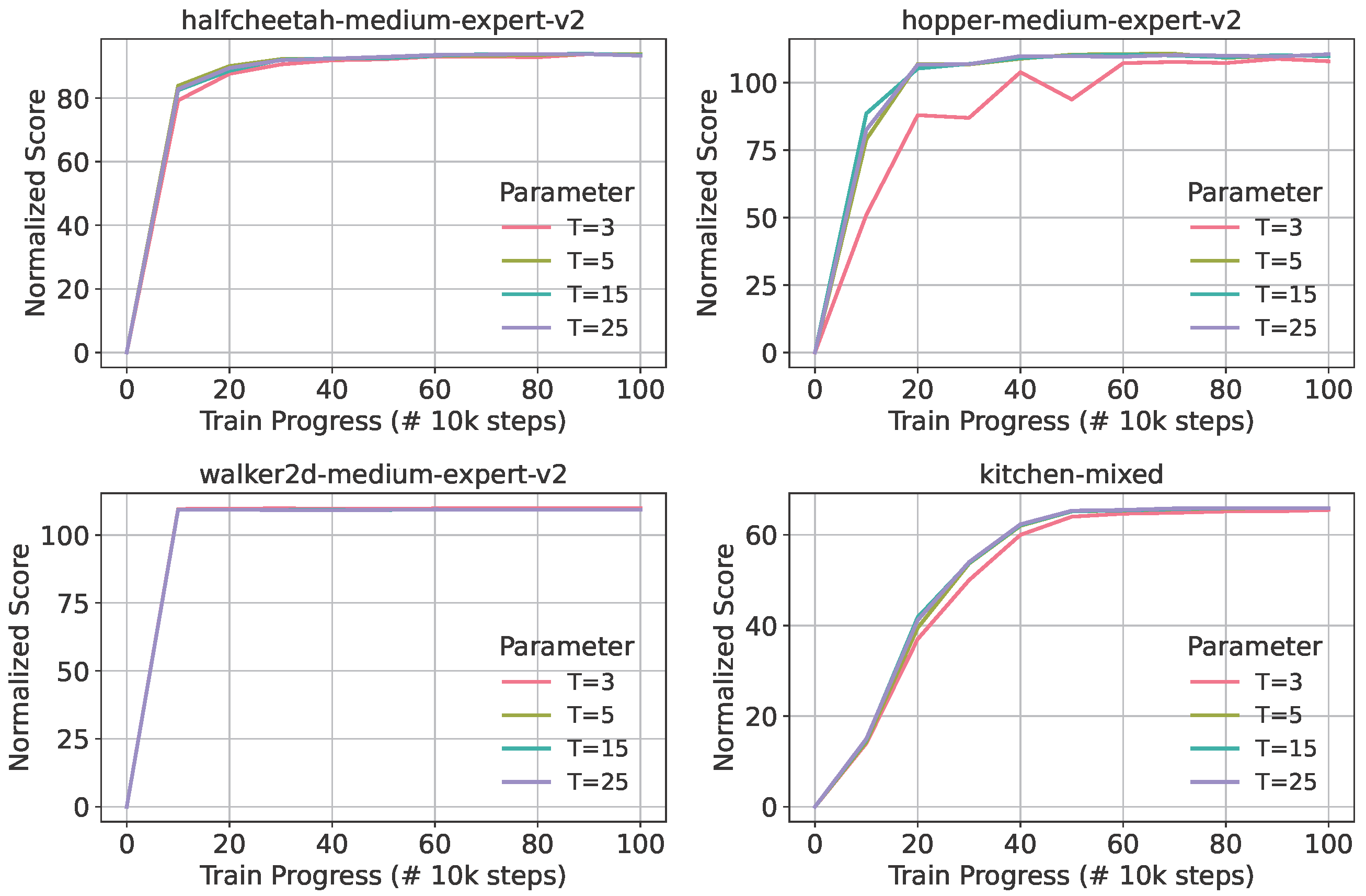
The number of denoising steps, denoted as t, within diffusion models is a critical hyperparameter that significantly influences both the quality of generated samples and the efficiency of the inference process. Generally, increasing the number of denoising steps facilitates the progressive refinement of the output through more meticulous noise removal, thereby yielding samples characterized by enhanced fidelity and realism. Each successive step applies subtle adjustments to the generated data, with the cumulative effect leading to a sharper final result. However, each additional denoising step necessitates a distinct forward pass through the model, consequently increasing the total generation time. Thus, selecting the number of denoising steps involves a fundamental trade-off between generation quality and computational efficiency. In applications such as control systems where real-time performance is paramount, minimizing the value of t becomes essential. As depicted in Figure 2, empirical analysis conducted in this study indicates that setting $t=5$ achieves an optimal balance between sample quality and real-time performance requirements.

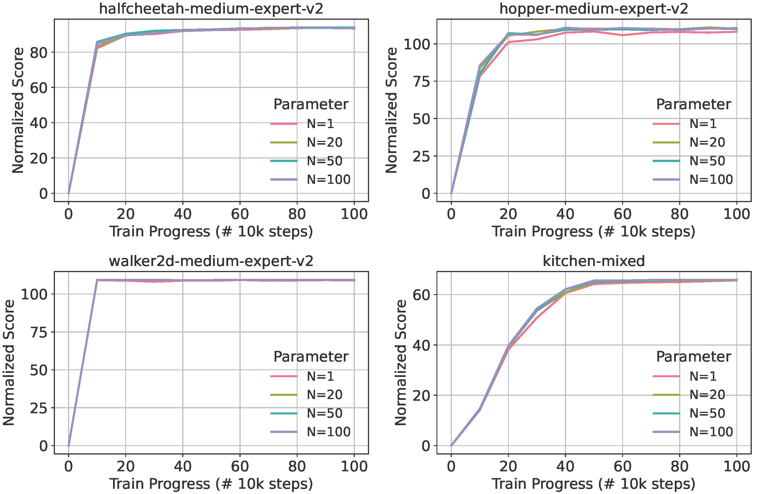
The alternative action parameter, denoted as n, governs the generation of N candidate actions for a given state s. These candidates are subsequently evaluated utilizing the learned critic $Q_{\varphi }$ prior to resampling the optimal action. This parameter similarly impacts both generation quality and computational efficiency. In principle, exploring multiple action candidates enables the model to select superior subsequent actions, potentially mitigating suboptimal local convergence and enhancing overall output quality. This process is analogous to conducting a broader search within the action space. While generating N candidate actions inherently demands greater computational resources compared to single-action generation, the parallelizable nature of this process renders the impact of N on generation speed less pronounced than that of t. Consequently, the parameter selection space for n typically affords greater flexibility. As demonstrated in Figure 3, experimental results indicate that setting $n=50$ optimally reconciles generation quality with real-time constraints.

4.3. Ablation Study

This section presents a comprehensive analysis validating the superior quantitative performance of Diffusion-Q Synergy (DQS) compared to other policy-constrained methods on D4RL benchmark tasks. Ablation studies were conducted to examine the two principal components of DQS: (1) the utilization of diffusion models as expressive policies and (2) Q-learning-guided denoising of suboptimal actions. Regarding the policy component, behavioral cloning comparisons were performed between the diffusion model and prevalent Transformer architectures. With respect to the Q-learning component, policy improvement was evaluated against BCQ methods.

As evidenced in

Table 3. Comparison of our diffusion model with CVAE models, and our Q-learning method with BCQ method.

Dataset	Diffusion vs. CVAE		Q-Synergy vs. BCQ
	CVAE-BC	Diffusion-BC	Diffusion-BCQ	DQS (Ours)
Medium-Replay-HalfCheetah	34.4	39.7	46.1	45.4
Medium-Replay-Hopper	84.7	92.8	94.7	96.1
Medium-Replay-Walker2d	67.3	71.4	90.9	95.8
Mixed-Kitchen	49	51.2	58.5	68.0
Average	58.9	63.8	72.6	76.3

, diffusion-based behavioral cloning (Diffusion-BC) demonstrates performance superior to that of baseline approaches. This outcome validates the diffusion policy’s greater expressiveness and enhanced capability in fitting data distributions within control domains. The performance advantage of DQS over Diffusion-BC substantiates that the Q-learning-guided denoising of suboptimal actions provides additional policy enhancement. Table 3 further reveals that the Q-learning component of DQS yields more significant policy improvement than baseline methods, such as BCQ. Collectively, these results demonstrate the synergistic interaction between DQS’s dual components, which culminates in superior overall performance.

We conducted systematic evaluations of the actions generated at each temporal step under a fixed sampling horizon (T = 5) within the experimental environment. As depicted in Figure 4, these actions are referred to as “Sampling samples”. Our analysis reveals that the action outputs of the diffusion policy exhibit predominant dependence on the terminal sampling step. Importantly, the implementation of guidance mechanisms at this final sampling stage yields substantial improvements in the quality of generated actions.

5. Conclusions

The critical challenges of distributional shift and complex policy distributions in offline RL are investigated in this paper. Through rigorous theoretical analysis, an equivalence is established between policy optimization and the reverse process of diffusion models. This enables the interpretation of dataset actions as actions from the optimal policy that have been contaminated by noise. Building upon this insight, DQS is proposed; this novel algorithmic framework addresses these fundamental limitations. Experimental evaluations conducted on the D4RL benchmark demonstrate that the proposed method achieves superior performance compared to state-of-the-art approaches across most tasks, while maintaining computational efficiency (diffusion steps = 5, candidate actions = 50). However, the empirical results reveal certain limitations, particularly high variance in D4RL scores, which indicates potential instability in policy optimization. To mitigate this issue, future research may consider incorporating consistency models and event-triggered sampling to balance sampling efficiency and performance. In summary, this work contributes a new theoretical perspective and represents a methodological advancement within the field of offline reinforcement learning.