Article

Research, Verification and Uncertainty Analysis of Aircraft Structural Load/Strain Testing

1
College of Aerospace Engineering, Nanjing University of Aeronautics and Astronautics, Nanjing 210016, China
2
College of Instrument Science and Opto-Electronics Engineering, Beijing Information Science & Technology University, Beijing 100101, China
*
Author to whom correspondence should be addressed.
Appl. Sci. 2025, 15(18), 10116; https://doi.org/10.3390/app151810116
Submission received: 19 July 2025 / Revised: 30 August 2025 / Accepted: 8 September 2025 / Published: 16 September 2025

Abstract

The load/strain time–history experienced by aircraft structures during service is crucial original input data for structural life reliability design, life extension, and health monitoring management. Accurately and reliably measuring the strain time–history of aircraft structures and their corresponding loading states is key. Aiming to improve upon the shortcomings of traditional airborne strain measurement methods, this paper proposes a key strain airborne measurement method suitable for load-bearing structures based on the characteristics and requirements of a certain type of aircraft load-bearing structure. An airborne multi-channel synchronous sampling test and acquisition system is designed and integrated for airborne measurement and acquisition of key strains and corresponding loading states of load-bearing structures. The main factors affecting the output of aircraft structure strain airborne measurements are summarized. Based on this, an uncertainty evaluation model for the airborne strain testing system is established, and the uncertainty of the output strain is quantitatively given using multivariate fuzzy evaluation. The key strain time–history of the load-bearing structure is obtained through flight measurement data collection and processing, and the collected strain history is analyzed in combination with simultaneously collected flight parameters. The results show that the proposed airborne strain measurement method and the integrated airborne strain measurement and acquisition system can reliably measure and reproduce the real loading history of the structure, providing reliable data support for structural damage estimation and life prediction management. It also provides an effective and practical reference for strain measurement of other aircraft structures.

1. Introduction

The service life of an aircraft structure is one of the important technical indicators of an aircraft. With the increasing costs of the manufacturing and maintenance of newly developed aircraft, the expected service life of aircraft has gradually been extended from an economic perspective. Correspondingly, the reliability and operational safety of aircraft structures have become more prominent. As the service environment faced by in-service aircraft becomes more complex, harsh, and uncertain, the structural damage accumulation rate will increase significantly, and the structural life consumption rate will also accelerate. To ensure that aircraft can fully exert their combat effectiveness and improve the combat effectiveness of the aircraft fleet, it is necessary to continuously monitor and evaluate in real time the loading history and load status of aircraft structures and their key components [1,2,3,4,5].
The purpose of aircraft load/strain measurement is to measure the complete load/strain time–history caused by external loads acting on the structure. On the one hand, through flight tests, the actual loading experience of aircraft structures during flight can be determined, and the correctness of ground test and theoretical analysis results can be verified. On the other hand, the measured data can be used to compile the load/stress spectra of various structural components, providing data support and a scientific basis for structural service life assessment, design modification, structural health monitoring, and management [2,3,4,5,6,7].
The electrical strain measurement method, as a widely used testing technology, has been applied in the load spectrum testing of multiple domestic and foreign aircraft models and related fields. Through flight tests, the load/time–history of structures such as aircraft wings, landing gears, and engines has been obtained [3,4,5,6,7], which truly reflects the loading status of aircraft structures during service. In addition, a high-resolution multi-channel dynamic strain observation system was constructed in seismic simulation experiments to obtain a high-density and high-precision dynamic strain field [8]. In structural load measurement, strain gauges are typically arranged in areas with uniform stress and low strain gradients, and a full-bridge configuration is used to connect to the circuit for data acquisition. Subsequently, ground-based load calibration tests are carried out to establish the mapping relationship between structural load input and strain output. In the measurement of key structural strains, strain gauges are placed on critical structural components or heavily loaded areas, such as hole edges and structural butt joints. Bridges excited by constant voltage or constant current sources are used for acquisition to obtain the strain time–history of the tested parts during actual flight.
Ideally, the strain gauge pasted onto the test component should only respond to the external load applied to the component without being affected by other factors. However, in practical engineering applications, the output of the strain bridge circuit varies not only with the external load but also with changes in the surrounding environment [9]. The error factors of the resistance strain gauge measurement system come from many sources, which can be roughly divided into several categories [10,11]: (1) strain gauge performance factors, including sensitivity coefficient, transverse effect, etc.; (2) external environmental factors, including the influence of the ambient temperature where the strain gauge is located; (3) time effect factors, including creep, hysteresis, number of cycles, etc.; (4) installation and operation factors, including adhesive, geometric dimensions and surface of the test part, bridge connection form, etc.; and (5) force thermal characteristic factors of the tested structure, including the temperature of the structure measuring point, surface roughness, etc.
For the uncertainty measurement in the process of structural stress and strain testing, H.B. Motra [10] and others analyzed the sources of uncertainty when using various technologies to measure the mechanical properties of materials and proposed an uncertainty analysis method for stress and strain measurement of steel structures. W. Montero et al. [11] introduced two methods to define uncertainty, GUF and MMC, and applied these two methods to the uncertainty analysis of stress determined by resistance strain gauges for strain. Haslbeck and Arpin-Pont, among others [12,13,14], have proposed a method using Monte Carlo simulation to estimate the influence of deviations and uncertainties caused by the following factors: uncertainty in strain gauge position, averaging effect, and transverse sensitivity error.
In this paper, we carry out relevant research on the airborne measurement of aircraft structure strain and its uncertainty. First, we review some cases and existing problems of aircraft structure strain airborne measurement and analyze the causes of these problems. On this basis, an improved airborne measurement method suitable for the key strain of aircraft load-bearing structure parts is proposed. The main factors affecting the output of aircraft structure strain airborne measurement are systematically summarized, and an uncertainty evaluation model of the airborne strain testing system based on multivariate fuzzy comprehensive evaluation is established to quantitatively evaluate the uncertainty of the strain testing system. Finally, the key strain time–history of the aircraft load-bearing structure parts is obtained by converting the measured code values, and the effectiveness and robustness of the measured strain are verified and analyzed.

2. Structural Strain Measurement Principle

In the actual measurement of aircraft structural load spectra, resistance strain gauges are often used to form a test bridge circuit for measuring the load or stress of the structures. The most used measurement circuit is the Wheatstone bridge [15]. When the structure is loaded and deformed, this change is transmitted to the resistance strain gauge pasted on the structure surface. The strain gauge changes its resistance, and the change in this resistance is linearly proportional to the elongation or shortening of the structure surface. Figure 1 shows a typical DC (Direct Current) constant voltage source excited Wheatstone bridge. R 1 ,   R 2 ,   R 3 , and R 4 are resistance strain gauges or fixed resistors. An input excitation voltage Eexc is applied across terminals AB, and the analog strain signal V out at terminals CD is the output of the bridge. When R i changes, the analog strain signal V out output by the bridge is as follows:
V out = R 1 + Δ R 1 R 3 + Δ R 3 R 2 + Δ R 2 R 4 + Δ R 4 R 1 + Δ R 1 + R 2 + Δ R 2 R 3 + Δ R 3 + R 4 + Δ R 4 E exc
If Δ R i is much smaller than R i , the higher-order terms can be removed to obtain the following:
V out = E exc 4 ( 1 χ ) Δ R 1 R 1 Δ R 2 R 2 + Δ R 3 R 3 Δ R 4 R 4
where χ = 1 / ( 1 + 2 / i = 1 4 R 1 / R 1 ) is the nonlinear coefficient of the test bridge.
When all bridge arms are strain gauges, the relationship between the output analog strain signal V out and the strain ε is as follows:
V out = E exc 4 F g ( 1 χ ) ε 1 ε 2 + ε 3 ε 4
where Fg is the gauge factor.
During the flight measurement process, the time–history values of V out collected by real-time measurement can be converted and calculated by Equation (3a) to obtain the comprehensive strain output Δ ε = ε 1 - ε 2 + ε 3 - ε 4 of the bridge, which is
ε = ε 1 ε 2 + ε 3 ε 4 = 4 V out E exc F g ( 1 χ )
For isotropic materials, the generalized Hooke’s law simplifies to the following under plane stress conditions:
σ x = E 1 ν 2 ε x + ν ε y σ y = E 1 ν 2 ε y + ν ε x τ xy = E 2 1 + ν γ xy γ xy = 2 ε xy
wherein σ x is the stress in the x direction, σ y is the stress in the y direction, and τ x y is the shear stress; ε x is the linear strain in the x direction, ε y is the linear strain in the y direction, γ x y is the engineering shear strain, and ε x y is the shear strain; E is the elastic modulus; and ν is Poisson’s ratio.
(1) If the directions of principal stresses σ 1 and σ 2 are known and perpendicular to each other, then the principal strains ε 1 and ε 2 along the principal stress directions are measured using a Wheatstone bridge circuit. Assuming that the principal strains ε 1 and ε 2 form an angle θ with the x-axis (counterclockwise is positive), then
ε x = ε 1 cos 2 θ + ε 2 sin 2 θ ε y = ε 1 sin 2 θ + ε 2 cos 2 θ γ xy = ε 2 ε 1 sin 2 θ
By means of Equation (3d), ε x ,   ε y , and γ x y are obtained, which are then substituted into Equation (3c) to derive stresses σ x ,   σ y , and τ x y .
(2) If the directions of the principal stresses σ 1 and σ 2 are unknown, the linear strains ε θ 1 ,   ε θ 2 , and ε θ 3 in any three known directions within the plane are measured using a Wheatstone bridge circuit. Assuming that θ 1 ,   θ 2 , and θ 3 are the angles between these linear strains and the x-axis (counterclockwise is positive), the equations are solved simultaneously to obtain the results.
ε θ 1 = ε x + ε y 2 + ε x ε y 2 cos 2 θ 1 + γ xy 2 sin 2 θ 1 ε θ 2 = ε x + ε y 2 + ε x ε y 2 cos 2 θ 2 + γ xy 2 sin 2 θ 2 ε θ 3 = ε x + ε y 2 + ε x ε y 2 cos 2 θ 3 + γ xy 2 sin 2 θ 3
Solving Equation (3e) yields ε x ,   ε y , and γ x y , which are then substituted into Equation (3b) to obtain stresses σ x ,   σ y , and τ x y .

3. Strain Airborne Measurement Cases and Existing Problems

In the strain measurement of previous aircraft models, two typical bridge configurations, shown in Figure 2 and Figure 3, were used to measure the strain time–history of the key structural components.
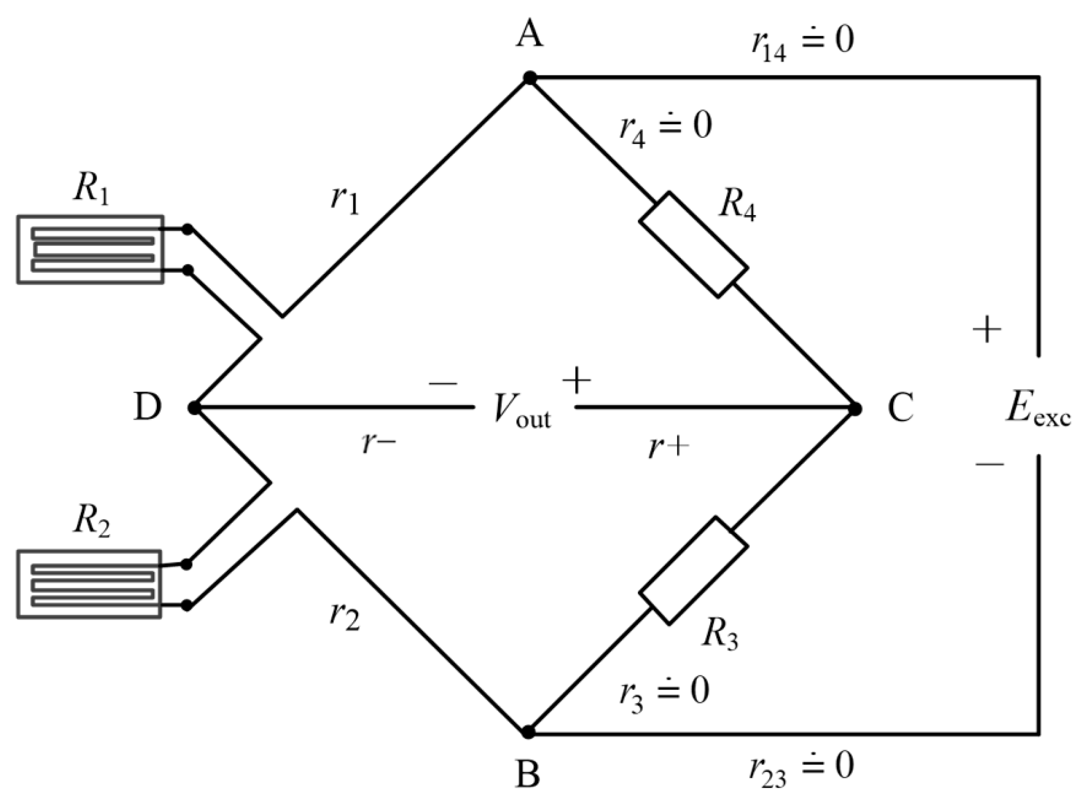
Figure 2 shows an airborne DC constant voltage source excited double-arm short-circuit test bridge. R1 is the working strain gauge arranged at the measuring point on the surface of the tested structure, and R 2   is the temperature compensation strain gauge placed on the compensation block near the working strain gauge. The positive terminal D of the output signal is connected to the signal terminal of the acquisition device, and the negative terminal C of the output signal is short-circuited with the casing, so the potential of point C is always equal to the potential of the casing.
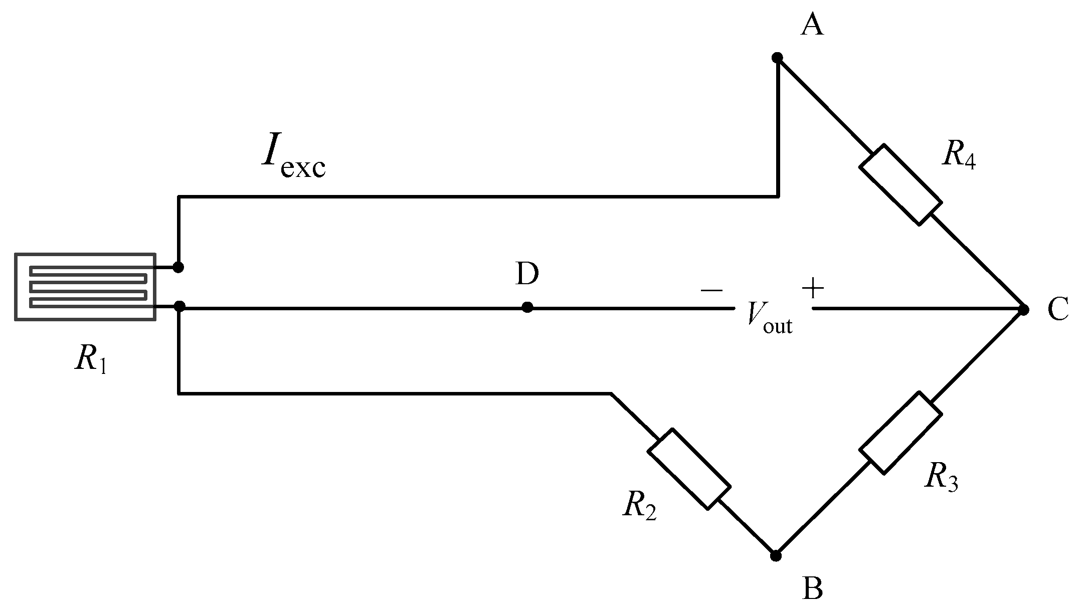
Figure 3 shows a constant current source excited single-arm bridge, where the strain gauge R 1 is connected to the bridge in a three-wire configuration. R 1 is the working strain gauge arranged at the measuring point on the surface of the tested structure. The current through the strain gauge R 1 remians constant, unaffected by lead wire resistance or strain gauge resistance. The resistance change Δ R 1 in the strain gauge is directly converted into the analog strain signal V out output at terminals CD, and the two show a linear proportional relationship. The reason for adopting this bridge design is that the structural test part does not have the space to arrange a temperature compensation strain gauge, or the environmental conditions where it is located do not allow for arranging a temperature compensation strain gauge and using a DC constant voltage source excitation.
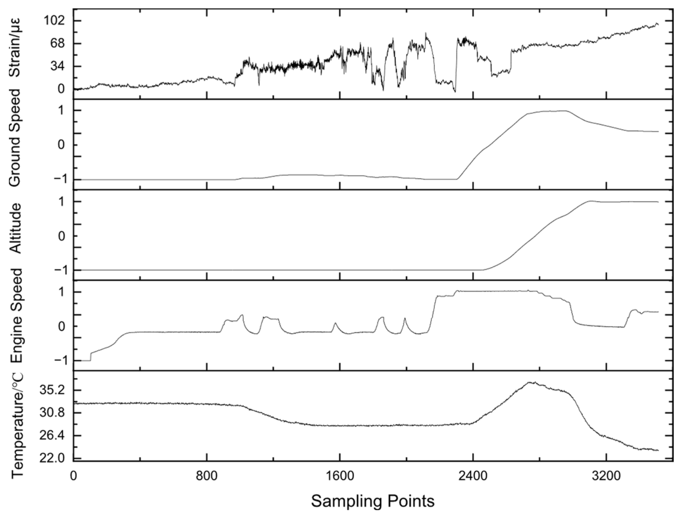
Figure 4 shows the time–history curves of key strains of the aircraft structure, along with ground speed, altitude, engine speed, and temperature, measured by the test bridge circuit shown in Figure 2 during the pre-takeoff ground segment and climb segment. All parameters have a sampling rate of 64 Hz, and the horizontal axis represents the sequence numbers of discrete sampling points in a single flight takeoff and landing.
It can be seen from Figure 4 that during the ground segment, the aircraft structure is not subjected to external loads, and the temperature fluctuation range is small, but the measured key structural strain shows a time-related drift trend. During the climb segment, the measured key structural strain also exhibits a time-related drift trend, which may be due to the increase in external loads on the structure or the decrease in temperature, leading to thermal strain in the output of the strain bridge circuit.
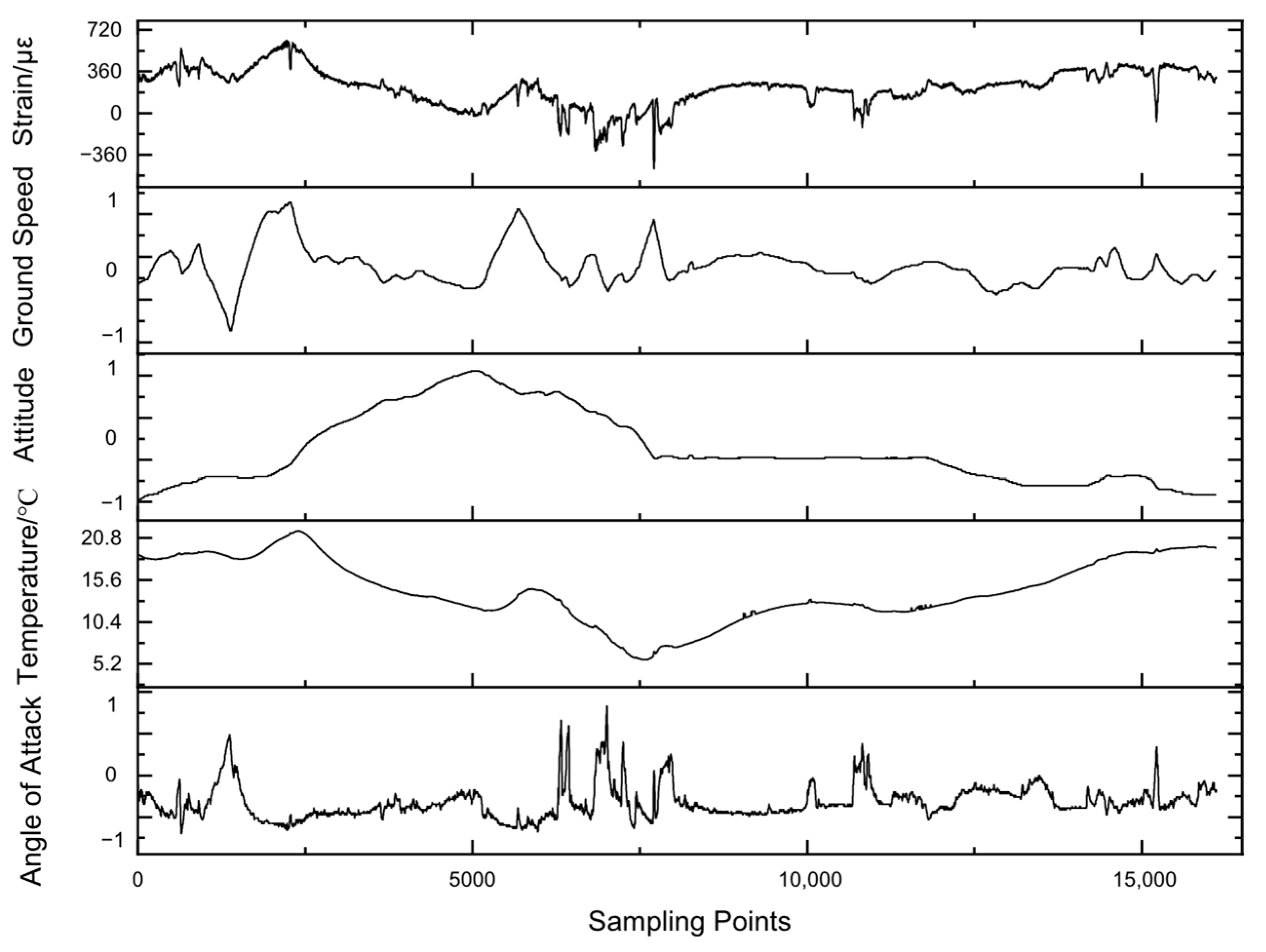
Figure 5 shows the time–history curves of key strains of the aircraft structure, along with ground speed, altitude, temperature, and angle of attack, measured by the test bridge circuit shown in Figure 3. All parameters have a sampling rate of 64 Hz, and the horizontal axis represents the sequence numbers of discrete sampling points in a single flight takeoff and landing.
It can be seen from Figure 5 that during the in-flight phase, temperature changes continuously due to variations in altitude and speed. The key structural strain shows a temperature-related trend: when the temperature decreases, the key structural strain decreases accordingly; when the temperature increases, the key structural strain increases. In addition, the key structural strain changes with the angle of attack. Overall, thermal strain caused by temperature changes constitutes the main component of the measured key structural strain.
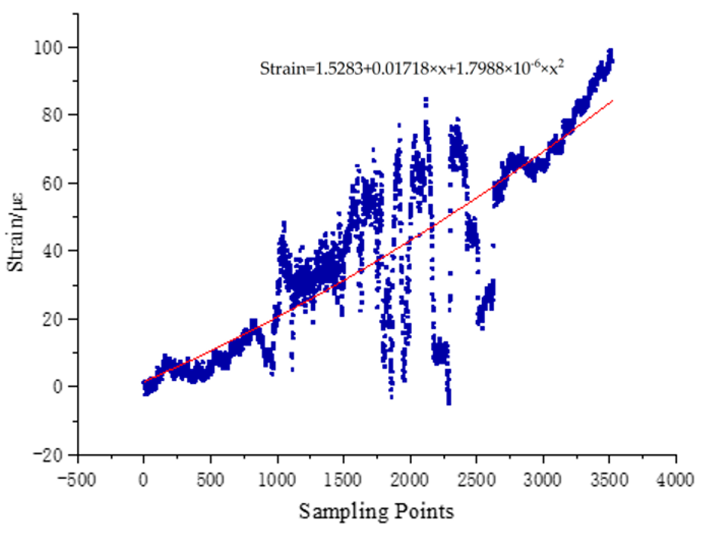
Utilizing the sampling point sequence numbers shown in Figure 4 as the horizontal axis (independent variable) and structural strain as the vertical axis (dependent variable), a scatter plot was drawn and fitted with a quadratic polynomial to obtain the variation law of structural strain over time, as shown in Figure 6. It can be seen from Figure 6 that the strain output by the bridge shows a significant drift trend over time from the start of the test system power supply.
With the temperature shown in Figure 5 as the horizontal axis (independent variable) and structural strain as the vertical axis (dependent variable), a scatter plot was drawn and fitted linearly to obtain the relationship between structural strain and temperature, as shown in Figure 7. It can be seen from Figure 7 that the strain output by the bridge has an obvious positive correlation with the ambient temperature, where ambient temperature fluctuations are mainly caused by altitude changes combined with maneuvering actions.
In Figure 6, the strain output by the bridge shows a drift trend over time from the start of the test system power supply. In Figure 7, the bridge output strain is obviously correlated with the ambient temperature, and the ambient temperature fluctuation is mainly caused by the superposition of altitude changes and maneuvering actions.
The problems existing in the abovementioned flight measurements will affect the accuracy and reliability of the strain data. The causes for this are summarized as follows:
(1)
Due to the resistance temperature effect of the strain gauge’s sensitive grid, the heating of the sensitive grid during normal operation will cause changes in its own resistance value, and real-time effective compensation cannot be performed due to the bridge characteristics;
(2)
According to Fourier’s law of heat conduction, the temperature of the sensitive grid will reach dynamic thermal equilibrium with its surrounding environment. Currently, there is a temperature gradient between the sensitive grid and the measured structural part, leading to inconsistent thermal deformation between the two, which causes thermal strain output;
(3)
In Figure 2, due to the resistance of the short-circuit wire, there is always a certain potential difference between point C and the casing, and this potential difference will change with the working state of the bridge and the external environment; that is, the zero point of the output signal will fluctuate during the entire airborne measurement process;
(4)
During the flight measurement process, there are differences in specimen materials, strain gauge pasting and protection processes, service environments, etc., between the thermal strain output results of the strain test bridge and the ground thermal output calibration test of the strain gauge. These differences may cause the actual thermal strain output of the strain gauge to deviate from the ground calibration thermal output curve or exceed the expected acceptable range, resulting in a significant increase in thermal strain output.

4. Improved Structural Strain Measurement Method

4.1. Structural Strain Measuring Point Location and Bridge Design

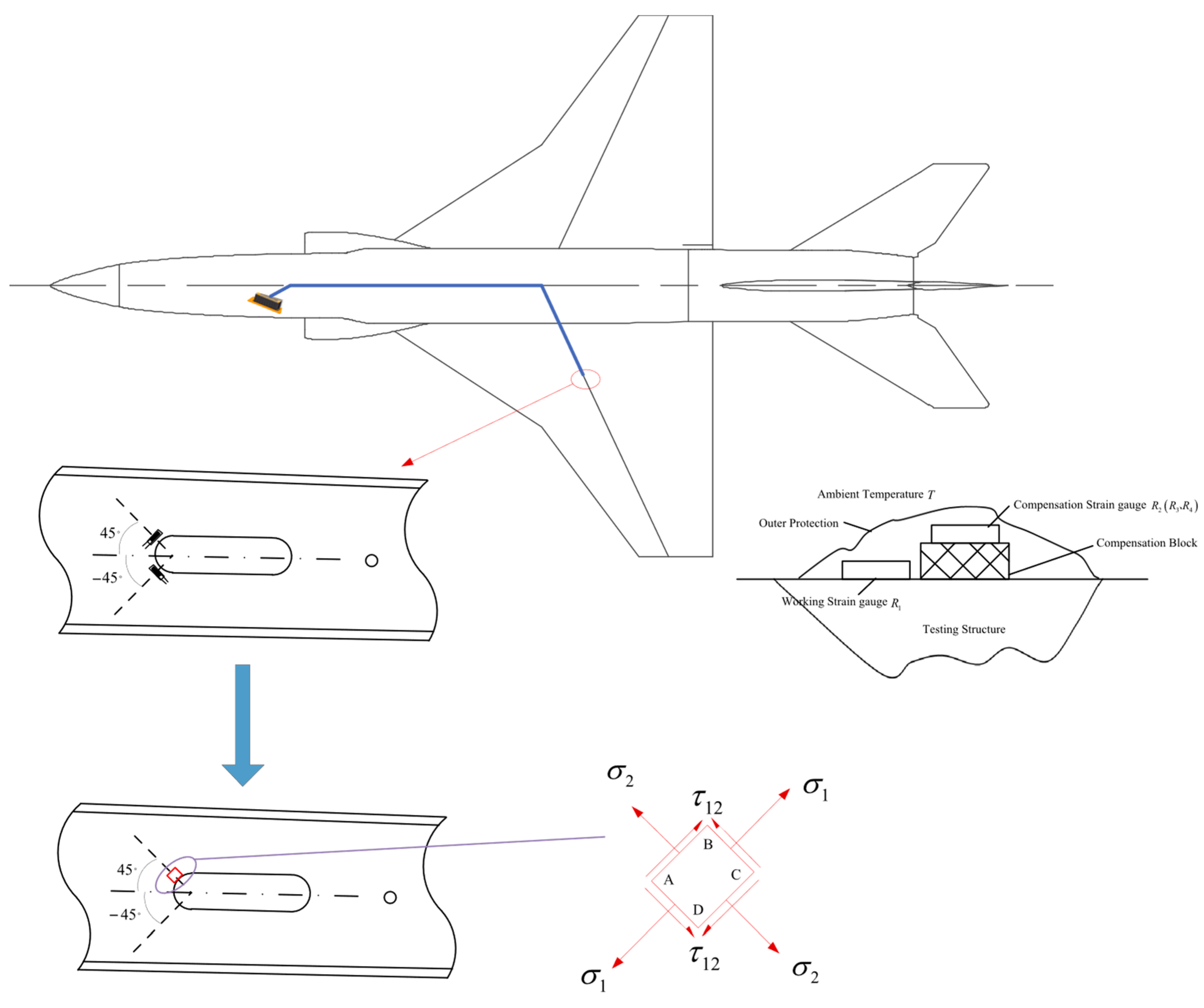
As shown in Figure 8, there is an oblong opening in the middle of the web of the load-bearing beam of the aircraft wing. To obtain the key strain time–history along the tangential direction at ±45° on the semicircular side of the hole through actual measurement, a tiny element is taken at the measuring point for in-plane force analysis. As shown in Figure 8, since the CD side of this tiny element is a free end face, it is easy to know that σ 1 0 , σ 2 = 0 , and τ 12 = 0 , and this strain measuring point is in a uniaxial stress state. Therefore, one set of uniaxial strain gauges R 1   is arranged close to the edge of the hole in each of the ±45° directions. And temperature compensation of the bridge circuit is carried out by arranging compensation strain gauges R 2   near the measuring point. The test cables are laid forward along the airframe to the test the acquisition system located near the cockpit of the front fuselage. Based on the strain test bridges shown in Figure 2 and Figure 3, the improved bridge design schemes for the strain measurement of the key parts of the aircraft structure are shown in Figure 9 and Figure 10. Figure 9 uses DC constant voltage as the bridge excitation. The working strain gauge R 1 and the compensation strain gauge R 2 are arranged at the structural test position end, and the low-temperature drift resistors R 3 and R 4 are used at the other end to form a Wheatstone test bridge. Figure 10 also uses DC constant voltage as the bridge excitation. Different from Figure 9, the working strain gauge R 1 and compensation strain gauges R 2 ,   R 3 , and R 4 at the structural test position directly form a Wheatstone test bridge, which is connected to the airborne strain test system.
R 1 is the working strain gauge, R 2 is the compensation strain gauge, and R 3 and R 4 are low-temperature drift resistors or strain gauges. The input excitation voltage E is applied to terminal AB, and the differential analog strain signal V out output by the bridge is at terminal CD. The resistance values are matched so that R 1 = R 2 and R 3 = R 4 . Currently, the bridge reaches an equilibrium state; that is, R 1 R 3 = R 2 R 4 .
Figure 9 uses DC constant voltage as the bridge excitation. A working strain gauge R 1 and a compensation strain gauge R 2 are arranged at the structural test position, and low-drift resistors R 3 and R 4 are used at the test acquisition system end to form a Wheatstone test bridge. r 1 and r 2 are the lengths of the test cables connected to the strain gauges, r 3 and r 4   are the lengths of the test cables connected to the low-drift resistors, and r 13 and r 14 are the lengths of the test cables connected to the excitation voltage E. It can be known that r 3 0 ,   r 4   0 ,   r 13 0 ,   r 14 0 , and E AB E exc .
Figure 10 also uses DC constant voltage as the bridge excitation. Different from Figure 9, the working strain gauge R 1 and compensation strain gauges R 2 , R 3 , and R 4 at the structural test position are directly used to form a Wheatstone test bridge, which is connected to the airborne strain test system. r 1   and r 2 ,   r 3 , and r 4 are the lengths of the test cables connected to the strain gauges, and r 13   and r 14   are the lengths of the test cables connected to the excitation voltage E exc . It can be known that r 1 , r 2 , r 3 , r 4 , r 13 , and r 14 are all not zero, and E AB < E exc .
When R i changes, the output analog strain signals V out of the test bridges shown in Figure 9 and Figure 10 are as follows:
V out = E AB 4 ( 1 χ ) Δ R 1 + Δ r 1 R 1 + r 1 Δ R 2 + Δ r 2 R 2 + r 2 + Δ R 3 R 3 Δ R 4 R 4
V out = E AB 4 ( 1 χ ) Δ R 1 + Δ r 1 R 1 + r 1 Δ R 2 + Δ r 2 R 2 + r 2 + Δ R 3 + Δ r 3 R 3 + r 3 Δ R 4 + Δ r 4 R 4 + r 4
where χ is the nonlinear coefficient of the test bridge; r is the resistance of the test cable from the acquisition channel to the strain gauge end; Δ r is the change in r ; and Δ R i is the change in the resistance value of R i . Correspondingly, the nonlinear coefficients χ of the test bridges are
χ 1 2 ( R 1 + r 1 R 1 + r 1 + R 2 + r 2 R 2 + r 2 + R 3 r 3 + R 4 r 4 )
and ,   χ 1 2 ( R 1 + r 1 R 1 + r 1 + R 2 + r 2 R 2 + r 2 + R 3 + r 3 R 3 + r 3 + R 4 + r 4 R 4 + r 4 )
The combination of temperature self-compensating strain gauges and bridge compensation methods is employed to reduce the thermal strain output caused by environmental temperature variations. Simultaneously, the output analog strain signals are converted into differential signals for acquisition and measurement, which significantly enhances the stability of the analog strain signals.

4.2. Multi-Channel Strain Testing System Construction and Calibration

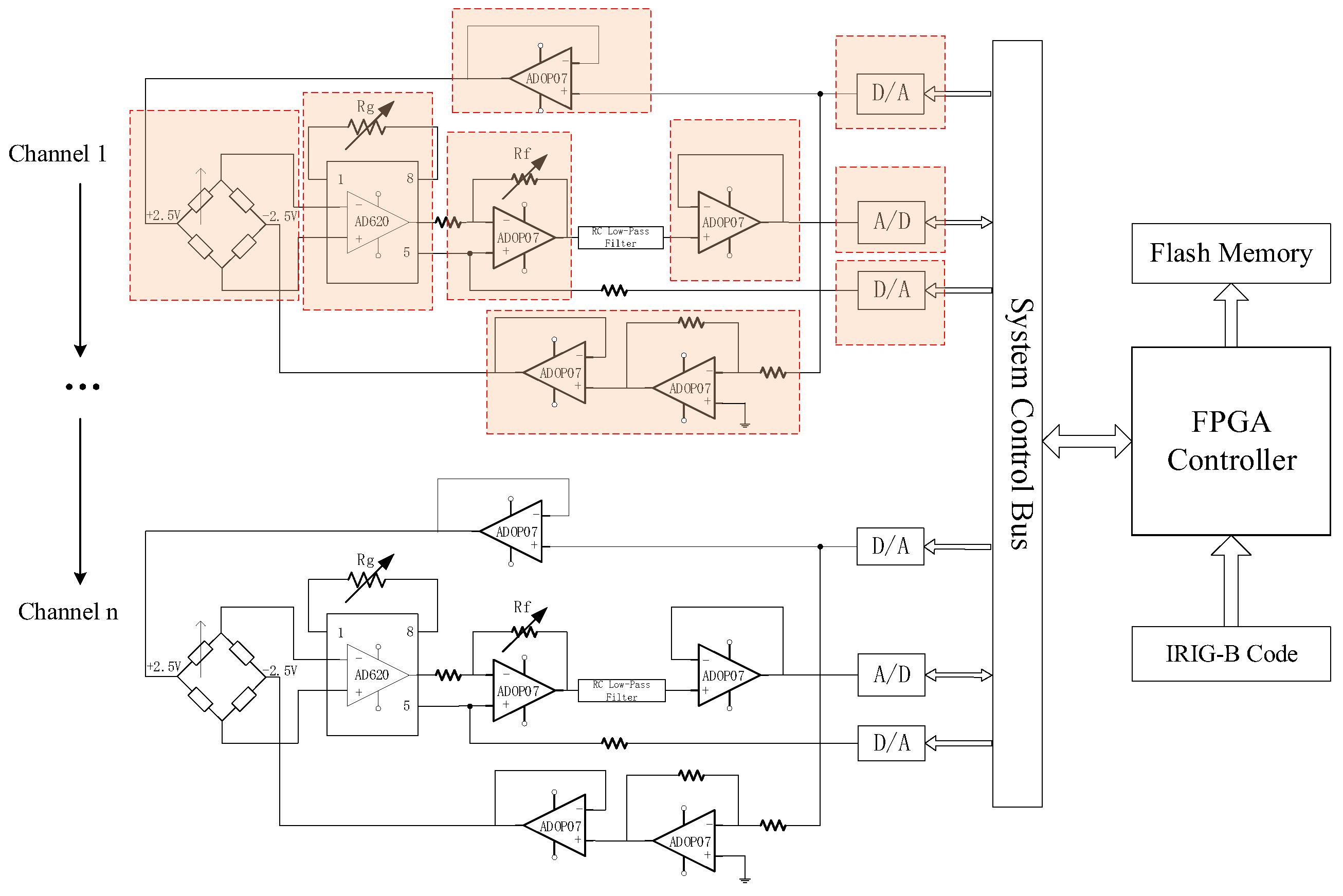
A programmable strain signal acquisition system with multi-channel synchronous sampling is constructed. The millivolt voltage signals generated by the Wheatstone strain bridges undergo two-stage amplification and filtering and are finally converted into digital signals via A/D (analog to digital) conversion for storage. The acquisition system is equipped with a serial interface for communication with a PC (personal computer). The FPGA (Field-Programable Gate Array) controller is programmed using host computer software to implement the system’s control logic and set acquisition parameters [16]. Key parameters for each channel, such as amplification gain, low-pass filter cutoff frequency, bias current, and sampling rate, can be independently configured via the host software [17]. The system incorporates an IRIG-B (Inter-Range Instrumentation Group-B) time code as the sampling clock for the A/D chips to achieve the synchronous sampling of all parameters. Data are encoded using PCM (Pulse Code Modulation) and stored as binary files on removable flash cards. Figure 11 illustrates the working principle of the multi-channel strain testing system.
The response process of the test acquisition system to structural strain signals includes the following parts: (1) the differential analog signal V out output by the strain bridge at the structural measurement point is transmitted to the collector end through the test cable; (2) the signal undergoes two-stage amplification and filtering processing by the collector; and (3) finally, it is converted into a digital signal via A/D conversion and stored. The total time of the above signal transmission and processing constitutes the system response time. Among them, the time for signal transmission, two-stage amplification, and A/D conversion is at the microsecond level, which is negligible compared to the filtering processing time. The strain signal sampling rate is 64 Hz, and an eighth-order Butterworth filter with a cutoff frequency of 16 Hz is used, so the filtering time is approximately 175 ms. Therefore, the system response time is approximately 175 ms.
The time synchronization accuracy between all channels of the test acquisition system is less than 300 ns, and when the strain sampling rate is set to 64 Hz, it is sufficient to ensure the time synchronization of all test signals.
The maximum excitation source noise of the test acquisition system is 0.01   mv rms , the full-scale range of the analog strain signal output by the bridge is 50 mv, the noise ratio is 0.01 mv rms 50 mv × 100 % = 0.125 FSR   (FSR stands for full-scale range), and the theoretical signal-to-noise ratio is SNR = 20 log 10 50 mv 0.01 mv rms = 74   dB .
To establish the mapping relationship between the structural strain ε and the analog strain signal V out , the analog strain signal V out output by the bridge is converted into a strain value. In underground room temperature conditions, the test cable from the strain gauge end to the collector end at the structural measurement point is considered a whole, and a standard strain source is used to calibrate the strain-to-analog strain signal coefficient η . The analog strain signal undergoes two stages of amplification and filtering and is finally converted into a digital signal by an AD converter. The code value-to-analog strain signal conversion coefficient ξ is obtained through calibration.
In Figure 12 and Figure 13, R A A ,   R B B ,   R C C ,   R D D denote the resistance value of the test cable from the strain gauge end at the structural measurement point to the collector end. Each test acquisition channel and its connecting wires are calibrated as an integral unit. The acquisition channel settings during calibration, including excitation voltage and gain coefficient, are maintained consistently with the actual measurement configuration. By adjusting the internal resistance of the strain source to output the standard strain ε c and synchronously recording the code value M c of the acquisition channel from the strain measurement system, the strain code value conversion coefficient ψ is obtained. In conclusion, the strain–analog strain signal coefficient η = ξ ψ can be derived.
The expression for η is as follows:
η = 1 E AB 4 R c R c + r K
where
R c is the internal resistance of the standard strain source; K is the set value of the sensitivity coefficient of the standard strain source.
In summary, the strain output expressions of the test acquisition channels for the bridges shown in Figure 9 and Figure 10 are, respectively, as follows:
ε = M ε c M c = E AB η 4 ( 1 χ ) Δ R 1 + Δ r 1 R 1 + r 1 Δ R 2 + Δ r 2 R 2 + r 2 + Δ R 3 R 3 Δ R 4 R 4
ε = M ε c M c = E AB η 4 ( 1 χ ) Δ R 1 + Δ r 1 R 1 + r 1 Δ R 2 + Δ r 2 R 2 + r 2 + Δ R 3 + Δ r 3 R 3 + r 3 Δ R 4 + Δ r 4 R 4 + r 4

5. Uncertainty Estimation of Strain Airborne Measurement Output

5.1. Influencing Factors of Strain Airborne Measurement Output

During actual flight tests, the bridge strain output value ε recorded by the airborne strain measurement system is composed of two components: one is the strain ε σ induced by the external mechanical loads borne by the structure and the other is the strain output ε T caused by temperature variations.
Thus, Equation (7a) can be decomposed into
ε = E AB η 4 1 χ Δ R 1 + Δ r 1 R 1 + r 1 Δ R 2 + Δ r 2 R 2 + r 2 + Δ R 3 R 3 Δ R 4 R 4 = E AB η 4 ( 1 χ ) Δ R 1 + Δ r 1 R 1 + r 1 σ Δ R 2 + Δ r 2 R 2 + r 2 σ + Δ R 3 R 3 σ Δ R 4 R 4 σ + E AB η 4 ( 1 χ ) Δ R 1 + Δ r 1 R 1 + r 1 T Δ R 2 + Δ r 2 R 2 + r 2 T + Δ R 3 R 3 T Δ R 4 R 4 T   = ε σ , 1 g ε σ , 2 g + ε σ , 3 g ε σ , 4 g + ε T , 1 g ε T , 2 g + ε T , 3 ρ ε T , 4 ρ = ε σ , 1 g + ε T , 1 - 2 g + ε T , 3 - 4 ρ
Similarly, Equation (7b) can be decomposed into
ε = E AB η 4 ( 1 χ ) Δ R 1 + Δ r 1 R 1 + r 1 Δ R 2 + Δ r 2 R 2 + r 2 + Δ R 3 + Δ r 3 R 3 + r 3 Δ R 4 + Δ r 4 R 4 + r 4 = E AB η 4 ( 1 χ ) Δ R 1 + Δ r 1 R 1 + r 1 σ Δ R 2 + Δ r 2 R 2 + r 2 σ + Δ R 3 + Δ r 3 R 3 + r 3 σ Δ R 4 + Δ r 4 R 4 + r 4 σ + E AB η 4 ( 1 χ ) Δ R 1 + Δ r 1 R 1 + r 1 T Δ R 2 + Δ r 2 R 2 + r 2 T + Δ R 3 + Δ r 3 R 3 + r 3 T Δ R 4 + Δ r 4 R 4 + r 4 T     = ε σ , 1 g ε σ , 2 g + ε σ , 3 g ε σ , 4 g + ε T , 1 g ε T , 2 g + ε T , 3 g ε T , 4 g   = ε σ , 1 g + ε T , 1 - 2 g + ε T , 3 - 4 g
where
ε σ , i g = E AB η 4 ( 1 χ ) Δ R i R i + r i σ , i = 1 , 2 , 3 , 4
ε σ , i g is the strain output of the strain gauge caused by the external mechanical loads borne by the structure
ε T , i g = E AB η 4 ( 1 χ ) Δ R i + Δ r i R i + r i T , i = 1 , 2 , 3 , 4
ε T , i g is the strain output of the strain gauge due to temperature variations
ε T , i ρ = E AB η 4 ( 1 χ ) Δ R i R i T , i = 3 , 4
ε T , i ρ is the strain output of the low-temperature drift resistor due to temperature changes.
To obtain the strain ε σ induced by external mechanical loads on the structure through strain airborne measurement, it is necessary to control the strain outputs ε T g and ε T ρ caused by temperature changes to be as small as possible and minimize their proportion in the total measured strain ε . Based on Equations (8a) and (8b), the main factors influencing the strain airborne measurement output are [9,14,18] the following:
(1)
Uncertainty of the channel excitation voltage E AB ;
(2)
Nonlinearity χ between the bridge output voltage V out and strain ε , especially significant when measuring large strains;
(3)
Difference between the strain ε output by the strain bridge and the strain ε c output by the standard strain source during calibration, affected by factors such as the transverse sensitivity effect of strain gauges, performance, and thickness of strain adhesive layers;
(4)
Dispersion of the strain channel calibration coefficient η ;
(5)
[ ( Δ R i + Δ r i ) / ( R i + r i )   ] T and ( Δ R i / R i )   T are affected by environmental temperature T changes, differences between adjacent bridge arm strain gauges R 1 and R 2 , low-temperature drift resistors R 3 and R 4 , or strain gauges R 3 and R 4 , as well as differences in linear expansion coefficients among sensitive grids, strain adhesive layers, and measured structural parts.

5.2. Summary of Influence Factors and Corresponding Variables

From the above analysis, the influencing factors of strain airborne measurement output involve many variables, with different primary and secondary effects, and different factors may include the same variable. Therefore, it is necessary to summarize the variables corresponding to each influencing factor and model and estimate the uncertainty of the strain airborne measurement output, which is of great significance for the improvement in the test system performance and data processing and analysis.
(1)
Expression of Structural Strain ε σ g
Considering the transverse effect coefficient H of the strain gauge and the strain transfer efficiency λ of the adhesive layer, the strain ε transmitted from the structural strain ε m to the sensitive grid of the strain gauge is
ε = 1 + ε ε m H 1 ν 0 H λ ε m
Substitute Equation (10) into Equation (9a) to obtain the structural strain ε σ g caused by mechanical loads as
ε σ g = E AB η 4 ( 1 χ ) R R + r F g 1 + ε ε m H 1 ν 0 H λ ε m = E AB η 4 ( 1 χ ) 1 + k F g 1 + ε ε m H 1 ν 0 H λ ε m
In the formula, ε m is the strain of the measured structural part along the testing direction; ε is the structural strain along the direction perpendicular to ε m ; F g is the gauge factor of the strain gauge; H is the transverse effect coefficient of the strain gauge; and λ is the strain transfer efficiency of the adhesive layer.
(2)
The expression for the thermal output ε T g ; of the strain gauge bridge arm
The thermal output of the strain gauge bridge arm R i i = 1,2 , 3,4 is expressed as strain ε T g ; that is,
ε T g = Δ R / R T F g = β g F g + g ( H ) α s α g Δ T
where g H = 1 + H 1 ν 0 H . Considering the strain transfer efficiency λ of the bottom layer and its linear expansion coefficient α a , Equation (12) can be written as follows:
ε T g = β g F g + g ( H ) α a α g + λ ( α s α a ) Δ T = β g F g + g ( H ) λ α s + 1 λ α a α g Δ T
By comparing Equation (12) and Equation (13), we obtain the following:
Δ R / R T = β g + g ( H ) F g α s α g + 1 λ α a α s Δ T
In the equations, Δ R R T is the relative resistance change rate; β g is the resistance temperature coefficient of the sensitive grid; α s is the linear expansion coefficient of the measured structural part; α g is the linear expansion coefficient of the sensitive grid; α a is the linear expansion coefficient of the strain adhesive layer; and ν 0 is the Poisson’s ratio of the structural material.
Specifically, when λ = 1 or α a = α s , Equation (13) degenerates into Equation (12).
Decompose Δ T into the temperature changes in the sensitive grid, the strain adhesive layer, and the measured structural part; that is,
Δ R / R T = β g g ( H ) F g α g Δ T g + g ( H ) F g α s Δ T s + ( 1 λ ) ( α a Δ T a α s Δ T s )
Simplifying Equation (15) gives the following:
Δ R / R T = β g g ( H ) F g α g Δ T g +   g ( H ) F g α s Δ T s 1 ( 1 λ ) ( 1 α a Δ T a α s Δ T s )
In Equation (16), Δ T g is the temperature change in the sensitive grid, Δ T a is the temperature change in the strain adhesive layer, and Δ T s is the temperature change in the measured structural part.
Based on Equation (16), considering the resistance r change in the test cable, the relative resistance change rate is
Δ R + Δ r R + r T = β g g ( H ) F g α g Δ T g + g ( H ) F g α s Δ T s 1 ( 1 λ ) ( 1 α a Δ T a α s Δ T s ) R + β r Δ T r r R + r
Let k = r R be the ratio of the test cable resistance to the strain gauge resistance. Simplifying Equation (17) gives
Δ R + Δ r R + r T = β g g ( H ) F g α g Δ T g + g ( H ) F g α s Δ T s ( 1 ( 1 λ ) ( 1 α a Δ T a α s Δ T s ) ) 1 1 + k + β r Δ T r k 1 + k
Substituting Equation (18) into (9b) to obtain the temperature strain of the strain gauge bridge arm R i i = 1,2 , 3,4 gives
ε T g = E AB η 4 ( 1 χ ) 1 + k β g g ( H ) F g α g Δ T g + g ( H ) F g α s Δ T s ( 1 ( 1 λ ) ( 1 α a Δ T a α s Δ T s ) ) + β r Δ T r k = E AB η 4 ( 1 χ ) 1 + k β g 1 + H 1 ν 0 H F g α g Δ T g + 1 + H 1 ν 0 H F g α s Δ T s ( 1 ( 1 λ ) ( 1 α a Δ T a α s Δ T s ) ) + β r Δ T r k
(3)
Expression for the thermal output ε T ρ of the low-temperature drift resistance bridge arm
Express the thermal output of the low-temperature drift resistance bridge arm R 3 or R 4 as strain ε T ρ ; that is,
ε T ρ = E AB η 4 ( 1 χ ) β R Δ T R
In Equation (20), β R is the temperature coefficient of the low-temperature drift resistance, and Δ T R is the temperature change in the low-temperature drift resistance.
The variables corresponding to the influencing factors of the strain airborne measurement output of the test system are summarized as shown in Table 1, which gives the median value, lower limit value, and upper limit value of each influencing variable.
Substitute the median values of various influencing variables in Table 1 into Equations (11), (19), and (20) and assume that χ = 0.01 ,   ε m = 1 μ ε ,   Δ T g = Δ T a = Δ T s = Δ T r = 1 °C.
(1)
Structural Strain Causedby Mechanical Loads ε σ _ ref g
For the strain measurement bridge circuit shown in Figure 9, the structural strain caused by mechanical loads is ε σ _ ref g = 0.985 μ ε ; for the strain measurement bridge circuit shown in Figure 10, the structural strain caused by mechanical loads is ε σ _ ref g = 0.987 μ ε . The structural strains caused by mechanical loads obtained from the strain measurement bridge circuits in Figure 9 and Figure 10 are consistent, and the strains obtained from the strain measurement bridge circuits are generally smaller than the actual strain values of the structure.
(2)
Thermal Output of Strain Measurement Bridge Circuit ε T _ ref g and ε T _ ref ρ
For the strain measurement bridge circuit shown in Figure 9, the strain output value under unit temperature change is ε T _ ref g = 25.713 μ ε , ε T _ ref ρ = 0.2 μ ε . In the thermal output of the strain gauge bridge arm ε T g _ ref , the thermal outputs caused by the characteristics of the strain gauge and the resistance change in the test cable are, respectively, as follows:
ε T _ ref g _ 1 = E AB η 4 ( 1 χ ) 1 + k β g 1 + H 1 ν 0 H F g α g Δ T g + 1 + H 1 ν 0 H F g α s Δ T s ( 1 ( 1 λ ) ( 1 α a Δ T a α s Δ T s ) )   = 1.437 μ ε ε T _ ref g _ 2 = E AB η 4 ( 1 χ ) 1 + k β r Δ T r k = 24.276 μ ε
The proportions of the two are ε T _ ref g _ 1 ε T _ ref g = 5.59 % and ε T _ ref g _ 2 ε T _ ref g = 94.41 % , respectively.
For the strain measurement bridge circuit shown in Figure 10, the strain output value under unit temperature change is ε T _ ref g = 2.657 μ ε . The thermal outputs caused by the characteristics of the strain gauge and the resistance change in the test cable are, respectively, as follows:
ε T _ ref g _ 1 = E AB η 4 ( 1 χ ) 1 + k β g 1 + H 1 ν 0 H F g α g Δ T g + 1 + H 1 ν 0 H F g α s Δ T s ( 1 ( 1 λ ) ( 1 α a Δ T a α s Δ T s ) )   = 1.440 μ ε ε T _ ref g _ 2 = E AB η 4 ( 1 χ ) 1 + k β r Δ T r k = 1.216 μ ε
The proportions of the two are ε T _ ref g _ 1 ε T _ ref g = 54.2 % and ε T _ ref g _ 2 ε T _ ref g = 45.8 % , respectively.
From the above analysis, it can be concluded that (1) compared with Figure 9, for the strain measurement bridge circuit shown in Figure 10, the thermal output of the bridge arm ε T _ ref g under unit temperature change is reduced by about 90%. (2) For the strain measurement bridge circuit shown in Figure 9, under unit temperature change, the proportion of the thermal output caused by the resistance of the test cable in the thermal output of the bridge arm is relatively large, while the proportion of the thermal output caused by the characteristics of the strain gauge is relatively small.

5.3. Uncertainty Measurement Based on Multivariate Fuzzy Comprehensive Evaluation

Due to the influences of measurement errors, manufacturing processes, and environmental factors, the impact variables summarized in Table 1 exhibit dispersions or uncertainties of varying degrees. In engineering practice, probabilistic methods such as probability density functions are often employed to describe variable uncertainties, treating impact variables as random variables for analysis. However, uncertainty is not equivalent to randomness; fuzziness and incertitude also constitute uncertainties. Probabilistic statistical density functions involving uncertain parameters require substantial statistical data as support or real-time acquisition and analysis via installed instruments, which often demands significant human and material resources for experiments, making it difficult to implement in practical engineering.
Through in-depth understanding of these impact variables or historical test data, the value ranges and membership degrees of these variables can be estimated. In this section, we describe these variables using fuzzy sets and establish an uncertainty measurement model for structural strain testing systems based on fuzzy sets. The measurement model adopts a multivariate fuzzy comprehensive evaluation method, which can evaluate the uncertainty of strain airborne measurement outputs affected by multiple factors and, on this basis, explore the variable factors that significantly influence strain airborne measurement outputs [19,20].

5.3.1. Establishment of Factor Set

Taking the influence variables summarized in Table 1 as the influencing factors of the multivariate fuzzy comprehensive evaluation, the factor sets for the output of resistance strain gauges and low-temperature drift resistance strain gauges are established, respectively, namely
U σ g = E AB , η , k , F g , H , λ , ν 0 , ε ε m U T g = E AB , η , k , F g , α a , α g , α s , β g , β r , H , ν 0 , λ , Δ T a , Δ T g , Δ T r , Δ T s U T ρ = E AB , η , β R , Δ T R

5.3.2. Determine Variable Weights

The second-order Taylor expansion of the multivariate function f x 1 , x 2 , x n at the point X = X 0 = x 01 , x 02 , x 0 n is given by
f X = f X 0 + f X 0 T X X 0 + 1 2 δ X T H X 0 δ X + O δ X δ X T   = f X 0 + f X 0 T δ X + 1 2 δ X T H X 0 δ X + O δ X δ X T  
In the formula, f X i = f x i , H X is the Hessian matrix and H X i j = 2 f x i x j , and O δ X δ X T is the second-order remainder term.
(1)
Variable weights of the structural strain ε σ g caused by mechanical loads
Performing the second-order Taylor expansion on ε σ g gives Expression (22); that is,
ε σ g   = ε σ g _ ref + i = 1 8 ε σ g U σ , i g δ U σ , i g + 1 2 i = 1 8 j = 1 8 2 ε σ g U σ , i g U σ , j g δ U σ , i g δ U σ , j g + O δ U σ g δ U σ g T = ε σ g _ ref + ε σ g E AB ε σ g ε ε m δ E AB δ ε ε m + 1 2 δ E AB δ ε ε m T 2 ε σ g E AB 2 2 ε σ g E AB ε ε m 2 ε σ g ε ε m E AB 2 ε σ g δ ε ε m 2 δ E AB δ ε ε m + O δ U σ g δ U σ g T = ε σ g _ ref + δ E AB δ ε ε m δ E AB 2 δ ε ε m 2 T a σ E AB a σ ε ε m a σ E AB 2 a σ ε ε m 2 + O δ U σ g δ U σ g T
Omitting the high-order terms of the second order and above, expanding Equation (22) gives
ε σ g = ε σ g _ ref + ψ E AB a σ E AB ζ E AB / 2 + + ψ ε ε m a σ ε ε m ζ ε ε m / 2 + ψ E AB 2 a σ E AB 2 ζ E AB 2 / 2 + + ψ ε ε m 2 a σ ε ε m 2 ζ ε ε m 2 / 2
In the formula, δ x = ψ x ζ x ,   ζ x = max x min x represents the difference between the maximum and minimum values of variable x . The value range of ψ x is 1,1 ; ψ x approaching 0 indicates that x is close to the median value; approaching 1 indicates that x is close to the minimum value; and approaching 1 indicates that x is close to the maximum value. a σ x ζ x 2 is the weight value of variable x . Table 2 lists the influencing variables with relatively large weights in the expression of ε σ g for the strain bridges in Figure 9 and Figure 10 and their corresponding weight values. The relative magnitude of the weight value indicates the sensitivity of the variable. A larger weight value means that when the variable changes by one unit due to uncertainty, the variation in the strain signal is greater, correspondingly implying higher uncertainty.
Since the component H ε ε m includes the variable H , the weight value of variable H is retained in the table.
(2)
Variable weights of the thermal output ε T g of the strain measurement bridge circuit
Performing the second-order Taylor expansion on ε T g gives Expression (24); that is,
ε T g   = ε T g _ ref + i = 1 12 ε T g U T , i g δ U T , i g + 1 2 i = 1 12 j = 1 12 2 ε T g U T , i g U T , j g δ U T , i g δ U T , j g + O δ U T g δ U T g T = ε T g _ ref + ε T g E AB ε T g λ δ λ δ E AB δ λ + 1 2 δ E AB δ λ T 2 ε T g E AB 2 2 ε T g E AB λ 2 ε T g λ E AB 2 ε T g δ λ 2 δ E AB δ λ   + O δ U T g δ U T g T = a Δ T a Δ T a + a Δ T g Δ T g + a Δ T r Δ T r + a Δ T s Δ T s + a Δ T a E AB Δ T a + a Δ T g E AB Δ T g + a Δ T r E AB Δ T r + a Δ T s E AB Δ T s δ E AB + + a Δ T a λ Δ T a + a Δ T g λ Δ T g + a Δ T r λ Δ T r + a Δ T s λ Δ T s δ λ + a Δ T a E AB 2 Δ T a + a Δ T g E AB 2 Δ T g + a Δ T r E AB 2 Δ T r + a Δ T s E AB 2 Δ T s δ E AB 2 & + a Δ T a λ 2 Δ T a + a Δ T g λ 2 Δ T g + a Δ T r λ 2 Δ T r + a Δ T s λ 2 Δ T s δ λ 2 + O δ U T g δ U T g T = a Δ T a + a Δ T a E AB δ E AB + + a Δ T a ν 0 δ λ + a Δ T a E AB 2 δ E AB 2 + a Δ T a ν 0 2 δ λ 2 Δ T a + a Δ T g + a Δ T g E AB δ E AB + + a Δ T g ν 0 δ λ + a Δ T g E AB 2 δ E AB 2 + a Δ T g ν 0 2 δ λ 2 Δ T g + a Δ T r + a Δ T r E AB δ E AB + + a Δ T r ν 0 δ λ + a Δ T r E AB 2 δ E AB 2 + a Δ T r ν 0 2 δ λ 2 Δ T r + a Δ T s + a Δ T s E AB δ E AB + + a Δ T s ν 0 δ λ + a Δ T s E AB 2 δ E AB 2 + a Δ T s ν 0 2 δ λ 2 Δ T s + O δ U T g δ U T g T = 1 δ E AB δ λ δ E AB 2 δ λ 2 T a Δ T a a Δ T g a Δ T r a Δ T s a Δ T a E AB a Δ T g E AB a Δ T r E AB a Δ T s E AB a Δ T a λ a Δ T a E AB 2 a Δ T a λ 2 a Δ T g λ a Δ T g E AB 2 a Δ T g λ 2 a Δ T r λ a Δ T r E AB 2 a Δ T r λ 2 a Δ T s λ a Δ T s E AB 2 a Δ T s λ 2 Δ T a Δ T g Δ T r Δ T s + O δ U T g δ U T g T = 1 δ E AB δ λ δ E AB 2 δ λ 2 T A T g Δ T a Δ T g Δ T r Δ T s + O δ U T g δ U T g T
Omitting the high-order terms of order two and above, the strain output caused by the temperature of the adjacent bridge arms of the test strain bridge circuit is as follows:
ε T , 1 - 2 g = ε T , 1 g ε T , 2 g = 0 δ E AB , 1 δ E AB , 2 δ ν 0 , 1 δ ν 0 , 2 δ E AB , 1 2 δ E AB , 2 2 δ λ 1 2 δ λ 2 2 T A T g Δ T a , 1 Δ T g , 1 Δ T r , 1 Δ T s , 1 + 1 δ E AB , 2 δ λ 2 δ E AB , 1 2 δ λ 2 2 T A T g Δ T a , 1 Δ T a , 2 Δ T g , 1 Δ T g , 2 Δ T r , 1 Δ T r , 2 Δ T s , 1 Δ T s , 2 = 0 δ E AB , 1 - 2 δ λ 1 - 2 δ E AB , 1 - 2 2 δ λ 1 - 2 2 T A T g Δ T a , 1 Δ T g , 1 Δ T r , 1 Δ T s , 1 + 1 δ E AB , 2 δ λ 2 δ E AB , 2 2 δ λ 2 2 T A T g Δ T a , 1 - 2 Δ T g , 1 - 2 Δ T r , 1 - 2 Δ T s , 1 - 2 = ε T , 1 - 2 g δ E AB , 1 - 2 , δ λ 1 - 2 2 + ε T , 1 - 2 g Δ T a , 1 - 2 , , Δ T s , 1 - 2
Similarly,
ε T , 3 - 4 g = ε T , 3 g ε T , 4 g = 0 δ E AB , 3 - 4 δ λ 3 - 4 δ E AB , 3 - 4 2 δ λ 3 - 4 2 T A T g Δ T a , 3 Δ T g , 3 Δ T r , 3 Δ T s , 3 + 1 δ E AB , 4 δ λ 4 δ E AB , 4 2 δ λ 4 2 T A T g Δ T a , 3 - 4 Δ T g , 3 - 4 Δ T r , 3 - 4 Δ T s , 3 - 4 = ε T , 3 - 4 g δ E AB , 3 - 4 , δ λ 3 - 4 2 + ε T , 3 - 4 g Δ T a , 3 - 4 , , Δ T s , 3 - 4
The first term ε T , 1 - 2 g δ E AB , 1 - 2 , δ λ 1 - 2 2 in Equation (25) is expanded as follows
0 δ E AB , 1 - 2 δ λ 1 - 2 δ E AB , 1 - 2 2 δ λ 1 - 2 2 T A T g Δ T a , 1 Δ T g , 1 Δ T r , 1 Δ T s , 1 = 0 ψ E AB , 1 - 2 ψ λ 1 - 2 ψ E AB , 1 - 2 2 ψ λ 1 - 2 2 T 0 ζ E AB ζ λ ζ E AB 2 ζ λ 2 T A T g Δ T a , 1 Δ T g , 1 Δ T r , 1 Δ T s , 1 = ψ E AB , 1 - 2 a Δ T a E AB ζ E AB Δ T a , 1 + a Δ T g E AB ζ E AB Δ T g , 1 + a Δ T r E AB ζ E AB Δ T r , 1 + a Δ T s E AB ζ E AB Δ T s , 1 + + ψ λ 1 - 2 2 a Δ T a λ 1 - 2 2 ζ λ 1 - 2 2 Δ T a , 1 + a Δ T g λ 1 - 2 2 ζ λ 1 - 2 2 Δ T g , 1 + a Δ T r λ 1 - 2 2 ζ λ 1 - 2 2 Δ T r , 1 + a Δ T s λ 1 - 2 2 ζ λ 1 - 2 2 Δ T s , 1
In the formula, δ x 1 - 2 = ψ x 1 - 2 ζ x ,   ζ x = max x min x represents the difference between the maximum and minimum values of variable x . The value range of ψ x is 1,1 ;   ψ x 1 - 2 approaching 0 indicates that the difference between x 1 and x 2 is small; conversely, approaching 1 indicates that the difference between x 1 and x 2 is large. a Δ T a x ζ x Δ T a , 1 + a Δ T g x ζ x Δ T g , 1 + a Δ T r x ζ x Δ T r , 1 + a Δ T s x ζ x Δ T s , 1 is the weight value of variable x .
The second term ε T , 1 - 2 g Δ T a , 1 - 2 , , Δ T s , 1 - 2 of Equation (25) is expanded as follows
1 δ E AB , 2 δ λ 2 δ E AB , 2 2 δ λ 2 2 T A T g Δ T a , 1 - 2 Δ T g , 1 - 2 Δ T r , 1 - 2 Δ T s , 1 - 2 = 1 δ E AB , 2 δ λ 2 δ E AB , 2 2 δ λ 2 2 T A T g ζ Δ T a ζ Δ T g ζ Δ T r ζ Δ T s ψ T a , 1 - 2 ψ T g , 1 - 2 ψ T r , 1 - 2 ψ T s , 1 - 2 = ψ T a , 1 - 2 a Δ T a + δ E AB , 2 a Δ T a E AB + + δ λ 2 a Δ T a λ + δ E AB , 2 2 a Δ T a E AB 2 + + δ λ 2 2 a Δ T a λ 2 ζ Δ T a + ψ T g , 1 - 2 a Δ T g + δ E AB , 2 a Δ T g E AB + + δ λ 2 a Δ T g λ + δ E AB , 2 2 a Δ T g E AB 2 + + δ λ 2 2 a Δ T g λ 2 ζ Δ T g + ψ T r , 1 - 2 a Δ T r + δ E AB , 2 a Δ T r E AB + + δ λ 2 a Δ T r λ + δ E AB , 2 2 a Δ T r E AB 2 + + δ λ 2 2 a Δ T r λ 2 ζ Δ T r + ψ T s , 1 - 2 a Δ T s + δ E AB , 2 a Δ T s E AB + + δ λ 2 a Δ T s λ + δ E AB , 2 2 a Δ T s E AB 2 + + δ λ 2 2 a Δ T s λ 2 ζ Δ T s
In the formula, δ x 1 2 = ψ x 1 2 ζ x , and ζ x = max x min x represents the difference between the maximum and minimum values of variable x . The value range of ψ x is 1,1 ;   ψ x 1 2 approaching 0 indicates that the difference between x 1 and x 2 is small; conversely, approaching 1 indicates that the difference between x 1 and x 2 is large. a x + δ E AB , 2 a x E A B + + δ λ 2 a x λ + δ E A B , 2 2 a x E A B 2 + + δ λ 2 2 a x λ 2 ζ x is the weight value of variable x .
The first term ε T , 3 - 4 g δ E AB , 3 - 4 , δ λ 3 - 4 2 and the second term ε T , 3 - 4 g Δ T a , 3 - 4 , , Δ T s , 3 - 4 in Equation (26) have the same variable weight values as in Equation (25). Table 3 lists the influencing variables with relatively large weights in the expression of ε T g for the strain bridges in Figure 9 and Figure 10 and their corresponding weight values. The relative magnitude of the weight value indicates the sensitivity of the variable. A larger weight value means that when the variable changes by one unit due to uncertainty, the variation in the strain signal is greater, correspondingly implying higher uncertainty.
(3) Variable weights of the thermal output ε T ρ of the strain measurement bridge circuit
Performing the second-order Taylor expansion on ε T ρ gives Expression (28); that is,
ε T ρ   = ε T ρ _ ref + i = 1 4 ε T ρ U T , i ρ δ U T , i g + 1 2 i = 1 4 j = 1 4 2 ε T ρ U T , i ρ U T , j ρ δ U T , i ρ δ U T , j ρ + O δ U T ρ δ U T ρ T = ε T ρ _ ref + ε T ρ E AB ε T ρ η ε T ρ β R ε T ρ Δ T R δ E AB δ η δ β R δ Δ T R T + 1 2 δ E AB δ η δ β R δ Δ T R T 2 ε T ρ E AB 2 2 ε T ρ E AB η 2 ε T ρ E AB β R 2 ε T ρ E AB Δ T R 2 ε T ρ η E AB 2 ε T ρ η 2 2 ε T ρ η β R 2 ε T ρ η Δ T R 2 ε T ρ β R E AB 2 ε T ρ β R η 2 ε T ρ η 2 2 ε T ρ β R Δ T R 2 ε T ρ Δ T R E AB 2 ε T ρ Δ T R η 2 ε T ρ Δ T R β R 2 ε T ρ Δ T R 2 δ E AB δ η δ β R δ Δ T R + O δ U T ρ δ U T ρ T
Omitting the high-order terms of order two and above, the strain output caused by the temperature of the adjacent bridge arms of the test strain bridge circuit is
ε T , 3 - 4 ρ = ε T , 3 ρ ε T , 4 ρ = 0 δ E AB , 3 - 4 δ η 3 - 4 δ β R , 3 - 4 δ E AB , 3 - 4 2 δ E AB , 3 - 4 δ η 3 - 4 δ E AB , 3 - 4 δ β R , 3 - 4 δ η 3 - 4 2 δ η 3 - 4 δ β R , 3 - 4 δ β R , 3 - 4 2 T a Δ T R a Δ T R E AB a Δ T R η a Δ T R β R a Δ T R E AB 2 a Δ T R E AB η a Δ T R E AB β R a Δ T R η 2 a Δ T R η β R a Δ T R β R 2 Δ T R , 3 + 1 δ E AB , 4 δ η 4 δ β R 4 δ E AB , 4 2 δ E AB , 4 δ η 4 δ E AB , 4 δ β R 4 δ η 4 2 δ η 4 δ β R 4 δ β R 4 2 T a Δ T R a Δ T R E AB a Δ T R η a Δ T R β R a Δ T R E AB 2 a Δ T R E AB η a Δ T R E AB β R a Δ T R η 2 a Δ T R η β R a Δ T R β R 2 Δ T R , 3 - 4 = 0 δ E AB , 3 - 4 δ η 3 - 4 δ β R , 3 - 4 δ E AB , 3 - 4 2 δ E AB , 3 - 4 δ η 3 - 4 δ E AB , 3 - 4 δ β R , 3 - 4 δ η 3 - 4 2 δ η 3 - 4 δ β R , 3 - 4 δ β R , 3 - 4 2 T A T ρ Δ T R , 3 + 1 δ E AB , 4 δ η 4 δ β R 4 δ E AB , 4 2 δ E AB , 4 δ η 4 δ E AB , 4 δ β R 4 δ η 4 2 δ η 4 δ β R 4 δ β R 4 2 T A T ρ Δ T R , 3 - 4 = ε T , 3 - 4 ρ δ E AB , 3 - 4 , δ β R , 3 - 4 2 + ε T , 3 - 4 ρ Δ T R , 3 - 4
The definition method of the variable weight values contained in the first term and the second term of Equation (29) is the same as that in Equation (25). Table 4 lists the influencing variables with non-zero weights in the expression of ε T ρ for the strain bridge in Figure 9 and their corresponding weight values. The relative magnitude of the weight value indicates the sensitivity of the variable. A larger weight value means that when the variable changes by one unit due to uncertainty, the variation in the strain signal is greater, correspondingly implying higher uncertainty.
By minimizing the difference in the thermal output between adjacent bridge arms, the overall thermal output of the strain bridge is minimized. From the thermal output expressions ε T , 1 - 2 g ,   ε T , 3 - 4 g , and ε T , 3 - 4 ρ of adjacent bridge arms, it can be seen that there are several main reasons for the unequal thermal output of adjacent bridge arms: (1) The force thermal properties of the strain gauges and fixed resistors used in adjacent bridge arms are inconsistent, such as differences in strain gauge sensitivity coefficient Fg, sensitive grid resistance temperature coefficient βg, etc. (2) The ambient temperatures of the strain gauges, fixed resistors, and test cables in adjacent bridge arms are inconsistent, and the greater the temperature difference, the greater the thermal output. (3) The bridge thermal output caused by differences in the linear expansion coefficients of the strain gauge sensitive grid, strain adhesive layer, and the tested structural part. (4) Differences in force thermal properties between the tested structure and the temperature compensation block.

5.3.3. Determination of Judgment Set and Membership Degree

Establish the judgment set is V = { v 1 (Small), v 2 (Relatively Small), v 3 (Medium), v 4 (Relatively Large), v 5 (Large) } for each factor, and this is quantitatively expressed as V = 1,2 , 3,4 , 5 T . The difference values between the strain and resistance corresponding variables of adjacent bridge arms change fluctuantly within a certain interval. The possibility of the value-taking of the difference values of variables is described by the fuzzy membership function; that is, the single-variable judgment matrix R. As shown in Table 5 and Table 6, a possible judgment value of the influencing variable and its difference value is given, respectively. If the interaction x i x j between variables x i and x j is considered, the judgment value of the interaction x i x j can be obtained according to the single-variable judgment matrix R.
The value of ψ x 1 - 2 corresponds one-to-one with the judgment value of x 1 - 2 : (1) if 0 ψ x 1 - 2 < 0.2 , its judgment value is v 1 (Small); (2) if 0.2 ψ x 1 - 2 < 0.4 , its judgment value is v 2 (Relatively Small); (3) if 0.4 ψ x 1 - 2 < 0.6 , its judgment value is v 3 (Medium); (4) if 0.6 ψ x 1 - 2 < 0.8 , its judgment value is v 4 (Relatively Large); and (5) if 0.8 ψ x 1 - 2 1 , its judgment value is v 5 (Large).

5.3.4. Fuzzy Comprehensive Evaluation

For the convenience of analysis, assume that
Δ T g , 1 = Δ T a , 1 = Δ T s , 1 = Δ T r , 1 = 1 ° C , Δ T R , 3 = 1 ° C , x = E AB , λ , E AB 2 λ 2 , δ x , 4 = ζ x 2 , x = η , β R , δ x , 2 = ζ x 2 .
Use the weighted average model M = , + to calculate the comprehensive judgment B of the uncertainty of the strain output as B = b 1 b 2 b 3 b 4 b 5 = A R , and normalize B to obtain B ~ = b ~ 1 b ~ 2 b ~ 3 b ~ 4 b ~ 5 , b ~ i = b i j = 1 5 b j , i = 1 5 b ~ i = 1 .
The judgment set is V = { v 1 (Small), v 2 (Relatively Small), v 3 (Medium), v 4 (Relatively Large), v 5 (Large) }, and this is quantitatively expressed as V = 1,2 , 3,4 , 5 T ; then, the score of the evaluation item is S   =   B ~ V .
Table 7 shows the normalized comprehensive judgment B ~ and score S of each evaluation item.
As can be seen from Table 7, for the evaluation item ε σ , 1 g , the normalized comprehensive judgment B ~ has a relatively large proportion in v 1 (Small) and v 2 (Relatively Small), and the score S is slightly greater than 2. This indicates that the uncertainty of the evaluation item ε σ , 1 g obtained from the judgment values of the influencing variables in Table 2 is at a relatively small level.
For the evaluation items ε T , 1 - 2 g ,   ε T , 3 - 4 ρ , and ε T , 3 - 4 g , the normalized comprehensive judgment B ~ has a relatively large proportion in v 1 (Small) and v 2 (Relatively Small), and the score S is between 1 and 2. This indicates that the uncertainty of the evaluation items ε T , 1 - 2 g ,   ε T , 3 - 4 ρ , and ε T , 3 - 4 g obtained from the judgment values of the influencing variables in Table 3 are at a small level. The score S of each evaluation item depends on the distribution of the judgment values of the influencing variables. If the evaluation values are distributed towards v 1 (Small) and v 2 (Relatively Small), then the score S will be correspondingly smaller. However, if the evaluation values are distributed towards v 4 (Relatively Small) and v 5 (Large), then the score S will be correspondingly larger.
In practical engineering applications, the mechanical and thermal properties of the strain gauges on adjacent bridge arms, or fixed resistance values, compensation blocks, and the measured structure, test cables, etc., in Table 2 and Table 3 should be kept consistent, and the environmental temperature changes in these parts should also be kept as consistent as possible. Then, the output uncertainty of the constructed strain testing system will be greatly reduced, ensuring the accuracy and reliability of the aircraft structure strain testing.

6. Flight Test Verification and Statistical Analysis

6.1. Measured Strain Time–History

The strain time–history of the structural test location is obtained by converting the original measured strain code values into physical quantities. Figure 14 shows the synchronous time–history curves of the airborne measured strain of the structure during flight takeoff and landing, along with flight parameters such as normal overload, altitude, ground speed, and temperature, covering mission segments including pre-takeoff ground segment, climb segment, in-flight maneuver segment, descent segment, and landing ground segment. All parameters have a sampling rate of 64 Hz, and the horizontal axis represents the sequence numbers of discrete sampling points in the flight takeoff and landing.
It can be obtained from the figure that (1) the measured structural strain has a high correlation with the normal load factor throughout the flight process, and (2) in the ground segment, from the start of the data collection on the test system to before the aircraft accelerates and leaves the ground, the strain at the measurement location is near zero, while in the air segment, when the ambient temperature changes greatly, the strain at the measurement location does not show an obvious trend related to temperature changes.

6.2. Strain and Flight Parameters Statistical Analysis

The loads and strains endured by an aircraft structure are closely related to its flight conditions, which can be described by a set of flight parameters. To verify the effectiveness of the structural airborne strain measurement method proposed in this paper and its test results, the variation law of structural airborne strain with flight conditions is analyzed and discussed, and the effectiveness evaluation criteria are proposed: (1) the measured strain can reflect the real loading condition of the structure; (2) the proportion of strain output related to ambient temperature in the measured strain should be as small as possible.
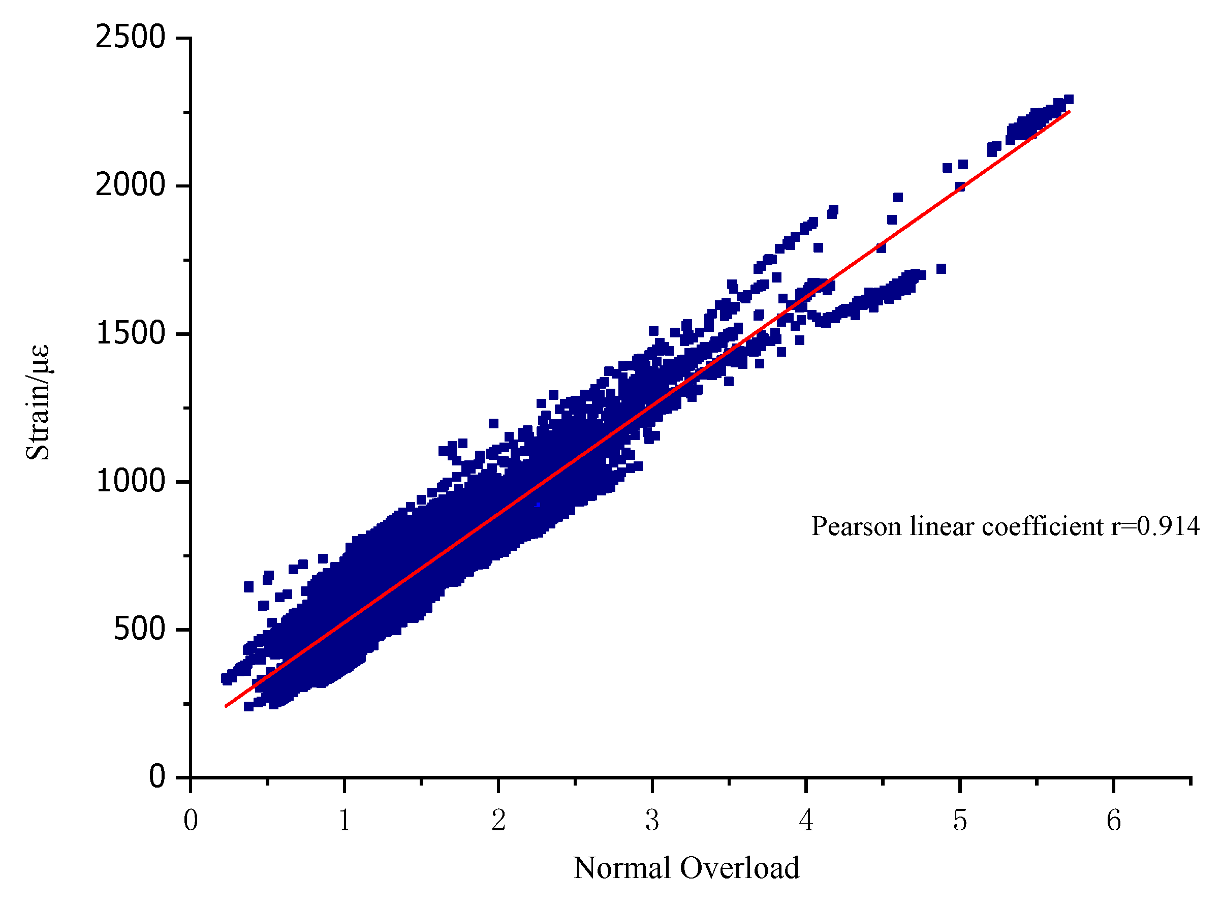
For the first evaluation criterion, the variation law between the measured strain and the corresponding flight parameters is analyzed to verify that the measured strain can reflect the real loading condition of the structure. The least squares fitting of the measured strain and overload shows from Figure 15 that there is a significant linear correlation between the measured structural strain and normal overload. The structural strain increment under a unit normal overload of 1 g obtained by linear fitting is Δ ε = 366.51 με.
For the second evaluation criterion, define the signal-to-noise ratio of the measured strain signal as t = ε σ ε T , which is the ratio of the structural strain caused by mechanical loads to the strain output caused by ambient temperature changes. The larger this value, the smaller the proportion of temperature-induced strain in the measured strain acquisition signal. Next, non-parametric correlation analysis is used to discuss the relative magnitude of the temperature-induced strain in the measured strain due to temperature changes.

6.2.1. Non-Parametric Partial Correlation Analysis PMIC

The relationship between structural strain and flight parameters is not a simple linear relationship but rather a complex nonlinear relationship, and the correlation between them is affected by multiple other factors together. Therefore, a non-parametric partial correlation coefficient PMIC based on the Maximal Information Coefficient (MIC) is adopted to control the influence of other variables on the two variables under investigation, to obtain the true correlation degree of the two variables [21,22,23,24]. The calculation method is as follows:
Given an ordered pair dataset D = x i , y i , i = 1,2 , n , and when the number of divided grids is less than or equal to B(n), its Maximal Information Coefficient (MIC) is defined as follows [23]:
MIC D = max AB B ( n ) I D , a , b log min a , b
In the formula, 0 < ε < 1 , ω 1 < B n O n 1 ε , all possible grid divisions of the dataset into a columns and b rows are denoted as G. The proportion of points in the dataset falling into the cells of G is approximately regarded as its probability distribution D|G, and the corresponding maximum mutual information is I D , a , b = m a x AB < B n I D G .
The non-parametric partial correlation coefficient PMIC based on MIC is defined as follows [24]:
PMIC X , Y | H Z = MIC R X , R Y = MIC X f ( Z ) , Y g ( Z )
In the formula, H(Z) is the hypothetical space on the variable set to be controlled, and f(Z) and g(Z) are the fitting functions of X and Y with respect to Z.

6.2.2. Result Analysis

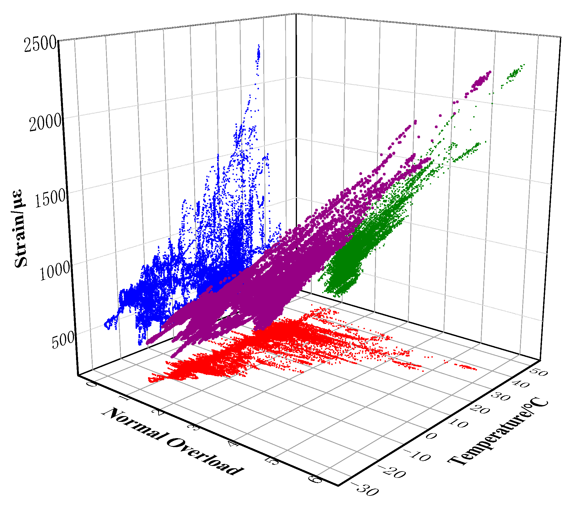
Figure 16 shows the 3D scatter points and projection diagram of the strain ε at the measurement point, load factor Ny, and temperature T collected during the takeoff and landing of the flight test. It can be seen from the figure that (1) the strain ε at the measurement point has a linear positive correlation with the normal load factor Ny. As the normal load factor Ny increases, the strain ε at the measurement point increases linearly accordingly; (2) the strain ε at the measurement point and the temperature T has a certain correlation; and (3) when the load factor Ny increases, the temperature T shows an increasing trend and the dispersion decreases.
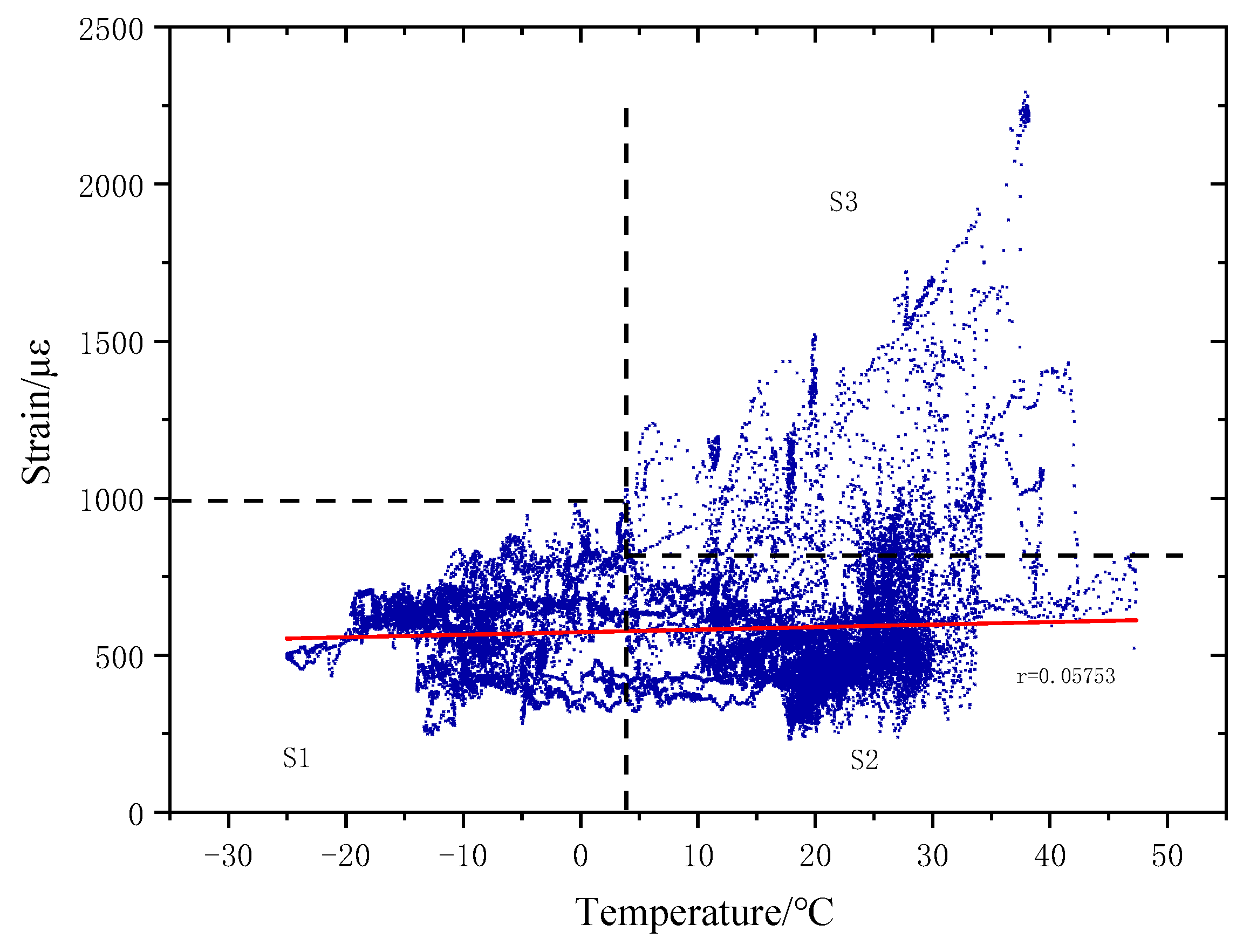
As shown in Figure 17, a scatter plot of measured strain ε versus temperature T from flight takeoff–landing data collection reveals that within the region S1 ∪ S2, the measured strain exhibits a nearly uniform distribution with temperature. In region S3, when the aircraft performs maneuvering actions, the altitude H decreases or the Mach number Ma increases, accompanied by an increase in the aircraft normal overload Ny. Since temperature T is related to altitude H and Mach number Ma, this results in a consistent variation trend between the measured strain and temperature T with certain dispersion. According to Equation (21), the maximum information coefficient M(D) = 0.2523 calculated for the measured point strain ε and temperature T can better reflect the correlation between the two compared to the Pearson linear coefficient r = 0.05753.
To obtain the true correlation between the measured strain ε and temperature T, the variable set Z = {Ny, Ma, H} is defined to control the combined influence of normal overload Ny, Mach number Ma, and altitude H on both strain and temperature T. Polynomials are used for nonlinear fitting of the measured strain ε and temperature T against the variable Z, and according to Equation (22), the partial multivariate information coefficient PMIC [measured strain ε, temperature T|H(Ny, Ma, H)] is 0.1302.
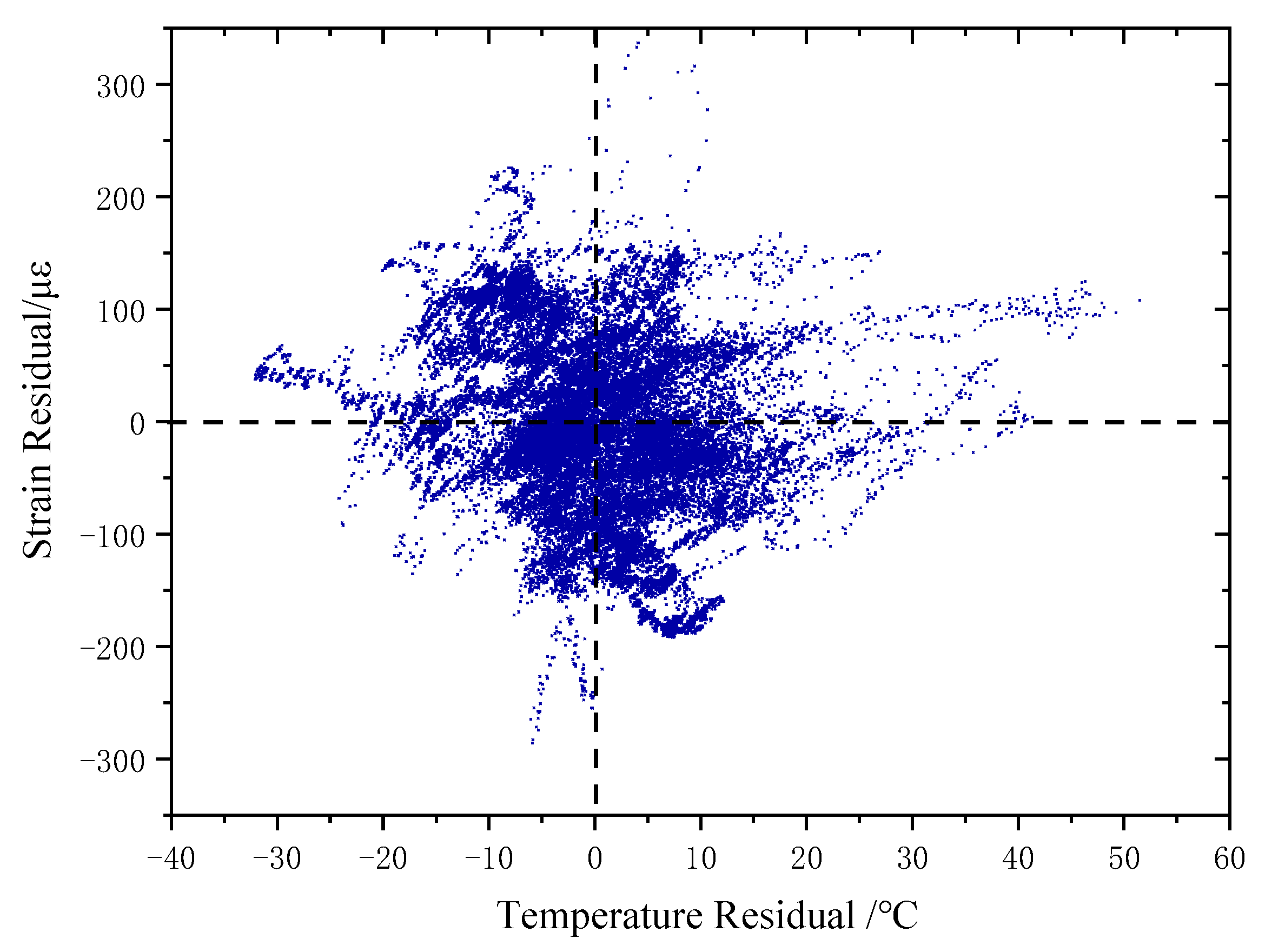
The scatter plot of measured strain residuals versus temperature residuals is shown in Figure 18, indicating essentially no correlation between the two across the entire region. As analyzed above, PMIC < M(D), suggesting that after controlling the influence of confounding variables, the correlation between measured strain ε and temperature T is further reduced, and temperature variation has a negligible effect on the strain measurements. The strain residuals at this point are caused by other influencing factors, such as roll rate and control surface deflection.

7. Conclusions

This paper proposes a strain testing method suitable for aircraft load-bearing structural parts, summarizes the main factors and variables affecting the output of aircraft strain testing, and presents a design method for aircraft structural load/strain testing bridge circuits and acquisition systems applicable to uncertain flight conditions. A multivariate fuzzy comprehensive evaluation method is adopted to quantitatively provide an uncertainty assessment of bridge strain signals affected by multiple factors. The variable factors that significantly influence bridge strain signals are analyzed and discussed. By controlling the fluctuation range of important influencing variables, the uncertainty of the system’s structural strain signal output can be reduced, and the accuracy and reliability of structural strain testing results can be improved.
The airborne strain measurement method for aircraft structures and the constructed airborne strain measurement and acquisition system have been successfully applied to the actual strain measurement of key parts of a certain type of aircraft load-bearing structure. The results show that (1) the measured structural strain ε has a high degree of correlation with the normal overload Ny throughout the entire flight process; (2) during the ground segment, from the start of data acquisition by the test system when powered on before the aircraft accelerates and leaves the ground, the strain ε at the measurement location fluctuates around zero; and (3) during the airborne segment, when the ambient temperature T changes significantly, the strain ε at the measurement location does not show a trend related to temperature T. This method can reliably measure and completely reproduce the real strain time–history endured by the aircraft structure.
This airborne structural strain measurement method and acquisition system can be applied to the strain testing of other aircraft models or structural components, including, but not limited to, fuselage frames, control surface shafts, landing gears, etc. Since the strain bridge signals arranged on the structure are affected by multiple factors such as the bridge configuration, strain gauges, test cables, the mechanical and thermal properties of the tested structure, and ambient temperature, it is necessary to select an appropriate bridge configuration according to the actual load form and service environment of the tested structure, summarize and analyze the variable factors that significantly affect the bridge strain signals, and control the fluctuation range of these important variables to significantly reduce the uncertainty of the structural strain testing output.
In future research, we plan to apply this airborne strain measurement method for aircraft structures and the constructed airborne strain measurement and acquisition system to strain the testing of other load-bearing structures under complex flight conditions. Focus will be placed on strain testing methods and their uncertainty modeling under conditions where the structure is subjected to multi-axial complex loads, the principal stress direction is unknown, and under different temperature change rates. This will yield a more realistic uncertainty assessment of bridge strain signals, aiming to achieve highly reliable measurement of the strain history at key structural parts.

Author Contributions

Conceptualization, W.X.; methodology, W.X.; software, H.H. and X.P.; validation, H.H.; formal analysis, W.X., H.H., X.P. and G.Y.; investigation, W.X.; resources, G.Y.; data curation, H.H., X.P. and G.Y.; writing—original draft, W.X.; writing—review and editing, G.Y.; Visualization, H.H. and X.P.; supervision, G.Y.; project administration, G.Y.; funding acquisition, W.X. All authors have read and agreed to the published version of the manuscript.

Funding

This research received no external funding.

Data Availability Statement

Restrictions apply to the datasets. The dataset presented in this article is not readily available as the data are part of an ongoing follow-up study. For requests to access the dataset, please contact email: yanguang79@bistu.edu.cn.

Conflicts of Interest

The authors declare no conflicts of interest.

Abbreviations

The following abbreviations are used in this manuscript:
DCDirect Current
V outAnalog Strain Signal
E excInput Bridge Excitation Voltage
E ABBridge Excitation Voltage between A and B
ŋStrain–Analog Strain Signal Coefficient
kRatio of Cable Resistance to Strain Gauge Resistance
F gGauge Factor
α aCoefficient of Thermal Expansion of Strain Adhesive Layer
α gCoefficient of Thermal Expansion of Sensitive Grid
α sCoefficient of Thermal Expansion of Tested Structural Part
β gTemperature Coefficient of Resistance of Sensitive Grid
β rTemperature Coefficient of Test Cable
H gTransverse Effect Coefficient of Strain Gauge
EElastic Modulus of Structural Material
ν0Poisson’s Ratio of Structural Material
λStrain Transfer Efficiency of Adhesive Layer
ΔTaTemperature Change in Strain Adhesive Layer
ΔTgTemperature Change in Strain Gauge Sensitive Grid
ΔTrTemperature Change in Test Cable
ΔTsTemperature Change in Tested Structural Part
β RTemperature Coefficient of Low-Drift Resistance
ΔTRTemperature Change in Low-Drift Resistance
ε ε m Ratio of Strain ε   to Strain ε m
RStrain Gauge Resistance
ΔRChange in Strain Gauge Resistance
χ Nonlinear Coefficient of the Test Bridge
I e x c Constant Current of Bridge Circuit
A/DAnalog to Digital
PCPersonal Computer
FPGAField-Programable Gate Array
IRIG-B Inter-Range Instrumentation Group-B
PCMPulse Code Modulation
McCode Value of the Acquisition Channel
ψ Strain Code Value Conversion Coefficient
η Strain–Analog Strain Signal Coefficient
KSet Value of the Sensitivity Coefficient of the Standard Strain Source
MICMaximal Information Coefficient
PMIC Non-parametric Partial Correlation Analysis

References

  1. Staszewski, W.; Boller, C.; Tomlinson, G.R. Health Monitoring of Aerospace Structures: Smart Sensor Technologies and Signal Processing; John Wiley & Sons Ltd.: Hoboken, NJ, USA, 2003. [Google Scholar]
  2. Gao, Z.T. Statistics Applied in Fatigue; National Defense Industry Press: Beijing, China, 1986; pp. 169–198. (In Chinese) [Google Scholar]
  3. Yan, C.L. Measurement Technology and Compilation Theory of Load-Spectrum for Airplane; Aviation Industry Press: Beijing, China, 2010; pp. 1–288. (In Chinese) [Google Scholar]
  4. Yan, C.L.; Su, K.X. Safety Life and Design with Damage Tolerance of Aircraft Landing Gear; Aviation Industry Press: Beijing, China, 2011; pp. 1–134. (In Chinese) [Google Scholar]
  5. Yan, C.L.; Zhang, S.M.; Zhuo, N.S.; Gao, Z.T. Mechanical Model and Data Processing of Load Measurement Test for The Air-plane’s Wing Structure. Acta Aeronaut. Astronaut. Sin. 2000, 21, 56–59. (In Chinese) [Google Scholar]
  6. William, A.L.; Olney, C.D.; Chen, T.; Crawford, N.D.; Stauf, R.; Reichenbach, E.Y.; Bessette, D. Strain-gage loads calibration testing of the active aeroelastic wing f/a-18 airplane. In Proceedings of the 22nd AIAA Aerodynamic Measurement Technology and Ground Testing Conference, St. Louis, MO, USA, 24–26 June 2002. [Google Scholar]
  7. Conners, T.; Sims, R. Full Flight Envelope Direct Thrust Measurement on a Supersonic Aircraft. In Proceedings of the 34th AIAA/ASME/SAE/ASEE Joint Propulsion Conference and Exhibit, Cleveland, OH, USA, 13–15 July 1998; p. 206560. [Google Scholar]
  8. Guo, L.L.; Liu, L.Q.; Liu, P.X. The application of multi-channel dynamic strain observation sysytem in earthquake simulation experiments. Seismol. Geol. 2014, 36, 929–938. (In Chinese) [Google Scholar]
  9. Israel, L.; Nesrin, S.-K. A review of uncertainty in flight vehicle structural health monitoring, diagnosis and con-trol: Challenges and opportunities. Prog. Aerosp. Sci. 2010, 46, 247–273. [Google Scholar]
  10. Motra, H.B.; Hildebrand, J.; Dimmig-Osburg, A. Assessment of strain measurement techniques to characterise mechanical properties of structural steel. Eng. Sci. Technol. Int. J. 2014, 17, 260–269. [Google Scholar] [CrossRef]
  11. Montero, W.; Farag, R.; Diaz, V.; Ramirez, M.; Boada, B.L. Uncertainties associated with strain-measuring system using resistance strain gauges. J. Strain Anal. Eng. Des. 2010, 46, 1–13. [Google Scholar] [CrossRef]
  12. Haslbeck, M.; Böttcher, J.; Braml, T. An Uncertainty Model for Strain Gages Using Monte Carlo Methodology. Sensors 2023, 23, 8965. [Google Scholar] [CrossRef] [PubMed]
  13. Arpin-Pont, J.; Gagnon, M.; Tahan, S.A.; Coutu, A.; Thibault, D. Strain gauge measurement uncertainties on hydraulic tur-bine runner blade. IOP Conf. Ser. Earth Environ. Sci. 2012, 15, 062042. [Google Scholar] [CrossRef]
  14. Arpin-Pont, J.; Gagnon, M.; Tahan, S.A.; Coutu, A.; Thibault, D. Methodology for estimating strain gauge measurement biases and uncertainties on isotropic materials. J. Strain Anal. Eng. Des. 2015, 50, 40–50. [Google Scholar] [CrossRef]
  15. Ma, L.C.; Feng, R.X.; Xu, D.B. Electrical Measurement for Strain and Technology of Sensing; China Metrology Press: Beijing, China, 2010; pp. 174–195. (In Chinese) [Google Scholar]
  16. Borko, J.; Dulnik, G.; Grzelka, A.; Luczak, A.; Paszkowski, A. A parametric synthesizer of audio signals on FPGA. Pomiary Autom. Kontrola 2015, 61, 367–369. [Google Scholar]
  17. Tong, S.B.; Hua, C.Y. Fundamentals of Analog Electronics; Higher Education Press: Beijing, China, 2015; pp. 276–296. (In Chinese) [Google Scholar]
  18. Richard, W.L. A New Correction Technique for Strain-Gage Measurements Acquired in Transient-Temperature Environments; NASA Technical Memorandum 3593; 1996. Available online: https://ntrs.nasa.gov/api/citations/19960016591/downloads/19960016591.pdf (accessed on 7 September 2025).
  19. Xie, J.J.; Liu, C.P. Fuzzy Mathematical Method and its Application; Machinery Industry Press: Beijing, China, 2018; pp. 143–156. (In Chinese) [Google Scholar]
  20. Ma, S.L.; Wang, J. The Fuzzy Method of Risk Analysis in R&D of Air-to-Air Missile. Acta Aeronaut. Astronaut. Sin. 2007, 28, 106–110. (In Chinese) [Google Scholar]
  21. Sheng, Z.; Xie, S.Q.; Pan, C.Y. Probability Theory and Mathematical Statistics; Higher Education Press: Beijing, China, 2001; pp. 109–143. (In Chinese) [Google Scholar]
  22. Reshef, D.N.; Reshef, Y.A.; Finucane, H.K.; Grossman, S.R.; McVean, G.; Turnbaugh, P.J.; Lander, E.S.; Mitzenmacher, M.; Sabeti, P.C. Detecting Novel Associations in Large Data Sets. Science 2011, 334, 1518–1524. [Google Scholar] [CrossRef] [PubMed]
  23. Reshef, Y.A.; Reshef, D.N.; Finucane, H.K.; Sabeti, P.C.; Mitzenmacher, M. Measuring Dependence powerfully and Equitably. J. Mach. Learn. Res. 2016, 17, 1–63. [Google Scholar]
  24. Tan, Q.H.; Jiang, H.J.; Ding, Y.M. Model Selection Methods Based on Maximum Information Coefficient of Residuals. Acta Math. Sci. 2014, 34B, 579–592. [Google Scholar] [CrossRef]
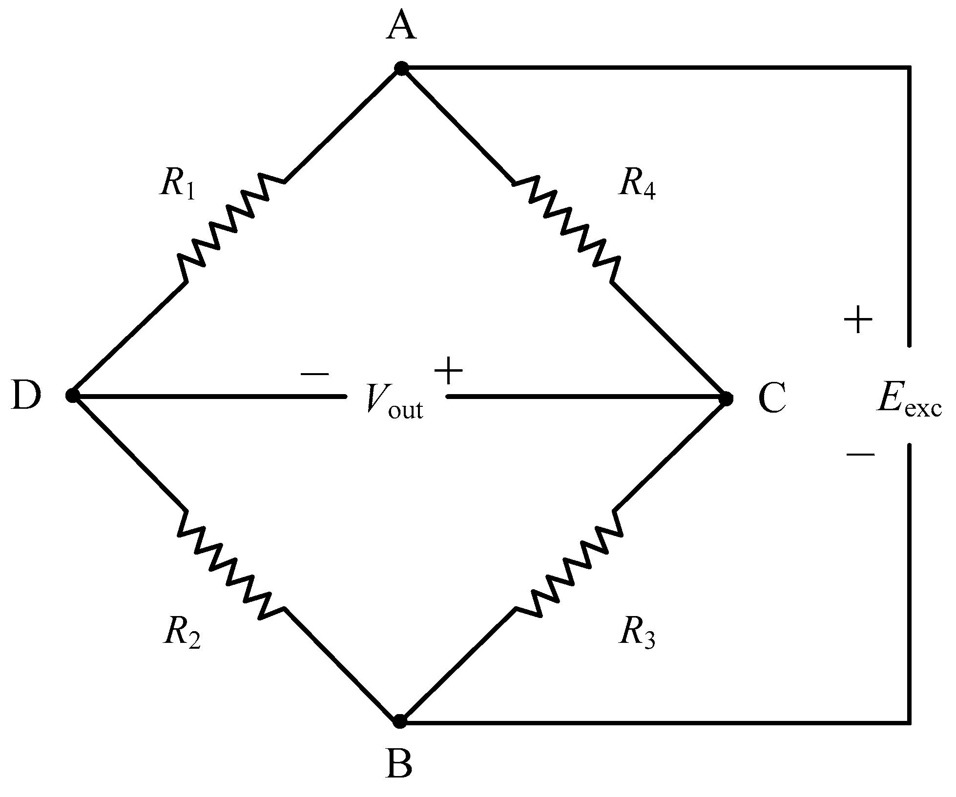
Figure 1. Typical DC constant voltage source excited Wheatstone bridge circuit.
Applsci 15 10116 g001
Figure 2. Airborne DC constant voltage source double-arm short-circuit test bridge circuit.
Applsci 15 10116 g002
Figure 3. Airborne constant current source excited single-arm test bridge circuit.
Applsci 15 10116 g003
Figure 4. Key strain and flight parameters time–history curve of aircraft structure measured by the method shown in Figure 2.
Applsci 15 10116 g004
Figure 5. Key strain and flight parameters time–history curve of aircraft structure measured by the test bridge shown in Figure 3.
Applsci 15 10116 g005
Figure 6. Drift trend of ground segment structural strain over time measured by the test bridge shown in Figure 2.
Applsci 15 10116 g006
Figure 7. Correlation between in-flight structural strain and temperature measured by the test bridge shown in Figure 3.
Applsci 15 10116 g007
Figure 8. Measuring point locations and strain gauge arrangements of aircraft wing structure.
Applsci 15 10116 g008
Figure 9. DC constant voltage source strain gauge and fixed resistor–four-arm test bridge circuit.
Applsci 15 10116 g009
Figure 10. DC constant voltage source strain gauge–four-arm test bridge circuit.
Applsci 15 10116 g010
Figure 11. Working principle diagram of multi-channel strain testing system.
Applsci 15 10116 g011
Figure 12. Block diagram of the bridge output strain calibration system shown in Figure 9.
Applsci 15 10116 g012
Figure 13. Block diagram of the bridge output strain calibration system shown in Figure 10.
Applsci 15 10116 g013
Figure 14. Synchronous time–history curves of measured structural strain and flight parameters.
Applsci 15 10116 g014
Figure 15. Scatter plot of measured strain and load factor and fitted curve.
Applsci 15 10116 g015
Figure 16. Three-dimensional scatter points and projection diagram of measured strain–load factor temperature.
Applsci 15 10116 g016
Figure 17. Scatter plot of measured strain vs. temperature.
Applsci 15 10116 g017
Figure 18. Scatter plot of measured strain residuals and temperature residuals.
Applsci 15 10116 g018
Table 1. Variables corresponding to summarized influencing factors.
Serial NumberVariables Corresponding to Influencing FactorsMedian ValueLower Limit ValueUpper Limit ValueRemarks
1Bridge Excitation Voltage EAB4.99 V4.99 V4.99 VCorresponds to Figure 9
4.89 V4.95 V4.82 VCorresponds to Figure 10
2Strain–Analog Strain Signal Coefficient η0.40450.40180.4073Corresponds to Figure 9
0.40920.40430.4152Corresponds to Figure 10
3Ratio of Cable Resistance to Strain Gauge Resistance k1.143 × 10−24.571 × 10−31.829 × 10−2Corresponds to Figure 9
5.714 × 10−41.143 × 10−41.029 × 10⁻³Corresponds to Figure 10
4Gauge Factor Fg2.122.2
5Coefficient of Thermal Expansion of Strain Adhesive Layer αa35.0 × 10−6/°C25.0 × 10−6/°C45.0 × 10−6/°C
6Coefficient of Thermal Expansion of Sensitive Grid αg15.2 × 10−6/°C10.2 × 10−6/°C20.2 × 10−6/°C
7Coefficient of Thermal Expansion of Tested Structural Part αs23.4 × 10−6/°C20.4 × 10−6/°C26.4 × 10−6/°C
8Temperature Coefficient of Resistance of Sensitive Grid βg−15.6 × 10⁻⁶/°C−20.6 × 10−6/°C−10.6 × 10−6/°C
9Temperature Coefficient of Test Cable βr0.0043/°C0.0038/°C0.0048/°C
10Transverse Effect Coefficient of Strain Gauge H0.3%0.10%0.50%
11Poisson’s Ratio of Structural Material ν00.30.250.35
12Strain Transfer Efficiency of Adhesive Layer λ0.950.91
13Temperature Change in Strain Adhesive Layer ΔTa---
14Temperature Change in Strain Gauge Sensitive Grid ΔTg---
15Temperature Change in Test Cable ΔTr---
16Temperature Change in Tested Structural Part ΔTs---
17Temperature Coefficient of Low-Drift Resistance βR0.4 × 10−6/°C0.35 × 10−6/°C0.45 × 10−6/°C
18Temperature Change in Low-Drift Resistance ΔTR---
19 Strain   Ratio   ε ε m −0.3−10.7
*Strain Gauge Resistance R350 Ω351.8 Ω348.2 ΩIncluded in k
*: Supplementary explanation.
Table 2. Weight values of variables influencing ε σ g .
Serial NumberVariableStrain Bridge in Figure 9Strain Bridge in Figure 10
Weight ValueWeight Value
1EAB01.2068 × 10−2
2η6.5773 × 10−31.1777 × 10−2
3k−6.6823 × 10⁻³−3.1799 × 10⁻³
4Fg4.6923 × 10−24.6834 × 10⁻²
5H−1.1102 × 10−190
6ν01.4794 × 10−41.4766 × 10−4
7λ5.1862 × 10−25.1764 × 10−2
8 ε / ε m 2.0712 × 10−32.0672 × 10−3
9Fg × λ2.4696 × 10−32.4748 × 10−3
10 H ×   ε / ε m 1.3820 × 10−31.3849 × 10−3
Table 3. Weight values of variables influencing ε T g .
Serial NumberVariableStrain Bridge in Figure 9Serial NumberVariableStrain Bridge in Figure 10
Weight ValueWeight Value
1k1.4394 × 10−51α g5.2174 × 10−6
2α a5.2065 × 10−62α s2.9739 × 10−6
3F g2.9677 × 10−63β g2.4748 × 10−6
4αsλ2.8228 × 10−64k9.7218 × 10−7
5Fg×αg2.4696 × 10−65λ6.0522 × 10⁻⁷
6ν0×λ1.6749 × 10−66αa×λ5.2174 × 10⁻⁷
7k×βr6.0395 × 10−77α a5.2174 × 10−7
8E AB05.2065 × 10−78F g4.3627 × 10−7
9αa×λ5.2064 × 10−79Fg×αg2.4845 × 10−7
10λ4.3535 × 10−710αs×λ1.5652 × 10⁻⁷
11k-ν02.4793 × 10−711Fg×αs1.4161 × 10−7
12β g1.7481 × 10−712β r1.4141 × 10−7
13ΔTa1.07 × 10−613ΔTa1.0931 × 10−6
14ΔTg−2.54 × 10−514ΔTg−2.5752 × 10⁻⁵
15ΔTr3.34 × 10−515ΔTr1.8289 × 10−6
16ΔTs2.59 × 10−516ΔTs2.6311 × 10−5
Table 4. Weight values of variables influencing ε T ρ .
Serial NumberVariableStrain Bridge in Figure 9
Weight Value
1η1.3585 × 10⁻⁹
2β R2.4978 × 10−8
3η-β R1.6982 × 10−10
4ΔTR2.8228 × 10−6
Table 5. Judgment values of influencing variables.
Serial NumberFactor Set UJudgment Set V
v 1 (Small) v 2 (Relatively Small) v 3 (Medium) v 4 (Relatively Large) v 5 (Large)
12345
1Bridge excitation voltage ΔEAB,1-00.80.2000
2Strain-simulated strain signal coefficient Δη,1-00.20.20.20.20.2
3Resistance ratio of cable and strain gauge Δk,1-00.20.20.20.20.2
4Gauge factor of strain gauge ΔFg,1-00.50.20.20.10
5Linear expansion coefficient of strain adhesive layer ΔH,1-00.50.20.20.10
6Expansion coefficient of sensitive grid wire Δν0,1-00.50.20.20.10
7Strain transfer efficiency of adhesive layer Δλ,1-00.30.30.20.10.1
8 Strain   ratio   ε ε m 0.20.20.20.20.2
Table 6. Judgment values of influencing variable differences.
Serial NumberFactor Set UJudgment Set V
v 1
(Small)
v 2 (Relatively Small) v 3 (Medium) v 4 (Relatively Large) v 5
(Large)
1Bridge excitation voltage ΔEAB,1-2 or ΔEAB,3-400000
2Strain-simulated strain signal coefficient Δη,1-2 or Δη,3-400000
3Resistance ratio of cable and strain gauge Δk,1-2 or Δk,3-40.70.20.100
4Gauge factor of strain gauge ΔFg,1-2 or ΔFg,3-40.50.20.20.10
5Linear expansion coefficient of strain adhesive layer Δαa,1-2 or Δαa,3-40.50.20.20.10
6Expansion coefficient of sensitive grid wire Δαg,1-2 or Δαg,3-40.50.20.20.10
7Coefficient of linear expansion of the measured structural part Δαs,1-20.40.20.20.10.1
Coefficient of linear expansion of the measured structural part Δαs,3-410000
8Temperature coefficient of the sensitive grid Δβg,1-2 or Δβg,3-40.50.20.20.10
9Temperature coefficient of test cable Δβr,1-2 or Δβr,3-40.70.20.100
10Transverse effect coefficient of strain gauge ΔH1-2 or ΔH3-40.50.20.20.10
11Poisson’s ratio of structural material Δν0,1-20.70.20.100
Poisson’s ratio of structural material Δν0,3-410000
12Strain transfer efficiency of the adhesive layer Δλ,1-2 or Δλ,3-40.30.30.20.10.1
13Temperature change in the strain adhesive layer ΔTa,1-20.40.20.20.10.1
Temperature change in the strain adhesive layer ΔTa,3-40.80.2000
14Temperature change in the strain gauge sensitive grid ΔTg,1-20.40.20.20.10.1
Temperature change in the strain gauge sensitive grid ΔTg,3-40.80.2000
15Temperature change in the test cable ΔTr,1-20.80.2000
Temperature change in the test cable ΔTr,3-40.80.2000
16Temperature variation in the tested structural part ΔTs,1-20.40.20.20.10.1
Temperature variation in the tested structural part ΔTs,3-40.80.2000
17Temperature coefficient of low-drift resistor ΔβR,3-40.70.20.100
18Temperature change in low-drift resistor ΔTR,3-40.80.2000
Table 7. Normalized comprehensive judgment B ~ and score S.
Serial NumberEvaluation Item Normalized   Comprehensive   Judgment   B ~ Score SRemarks
1 ε σ , 1 g δ E A B , , δ ε ε m 2 (0.382, 0.244, 0.195, 0.11, 0.069) 2.24Figure 9
2 ε σ , 1 g δ E A B , , δ ε ε m 2 (0.425, 0.239, 0.175, 0.099, 0.062) 2.135Figure 10
3 ε T , 1 - 2 g δ E A B , 1 - 2 , δ λ 1 - 2 2 (0.626, 0.194, 0.131, 0.038, 0.011) 1.596Figure 9
4 ε T , 1 - 2 g Δ T a , 1 2 , , Δ T s , 1 2 (0.781, 0.2, 0.009, 0.005, 0.005) 1.251Figure 9
5 ε T , 3 - 4 ρ δ E A B , 3 - 4 , δ β R , 3 - 4 2 (0.7, 0.2, 0.1, 0, 0) 1.4Figure 9
6 ε T , 3 - 4 ρ Δ T R , 3 - 4 (0.8, 0.2, 0, 0, 0) 1.2Figure 9
7 ε T , 1 - 2 g δ E A B , 1 - 2 , δ λ 1 - 2 2 (0.508, 0.202, 0.18, 0.085, 0.025) 1.861Figure 10
8 ε T , 1 - 2 g Δ T a , 1 2 , , Δ T s , 1 2 (0.61, 0.2, 0.095, 0.0475, 0.0475) 1.722Figure 10
9 ε T , 3 - 4 g δ E A B , 3 - 4 , δ λ 3 - 4 2 (0.636, 0.158, 0.138, 0.064, 0.004) 1.596Figure 10
10 ε T , 3 - 4 g Δ T a , 3 - 4 , , Δ T s , 3 - 4 (0.8, 0.2, 0, 0, 0) 1.200Figure 10
Disclaimer/Publisher’s Note: The statements, opinions and data contained in all publications are solely those of the individual author(s) and contributor(s) and not of MDPI and/or the editor(s). MDPI and/or the editor(s) disclaim responsibility for any injury to people or property resulting from any ideas, methods, instructions or products referred to in the content.