Article

A Study on the Application of Genetic Algorithms to the Optimization of Road Maintenance Strategies

Department of Civil Engineering, National Central University, Tao-Yuan 320317, Taiwan
*
Author to whom correspondence should be addressed.
Appl. Sci. 2025, 15(18), 10094; https://doi.org/10.3390/app151810094
Submission received: 18 August 2025 / Revised: 11 September 2025 / Accepted: 12 September 2025 / Published: 16 September 2025
(This article belongs to the Section Civil Engineering)

Abstract

This study proposes an optimization method that considers both section resurfacing and localized repairs of damaged points, based on the highly uneven distribution of pavement distress locations and under budget constraints. The model is formulated as an MILP (mixed-integer linear programming) model, where binary variables are used to simultaneously determine section resurfacing and localized repair actions. To overcome the excessive computation time required for large-scale road networks, a GA (genetic algorithm) is designed to perform heuristic searches. The model fully integrates information on distress locations, deduction values, and repair costs, and uses the maximization of the average PCI (pavement condition index) as the objective to ensure that decision-making focuses on tangible improvements in pavement service levels. Compared with the traditional point-by-point repair strategy, the proposed method can further increase the average PCI by approximately 3.5–4.0 points under medium- to high-budget conditions, demonstrating significant quantitative benefits. By simultaneously integrating section resurfacing and localized repair decisions, it saves about 10–15% more resources than individual repair methods while ensuring higher coverage of pavement distress. This method provides road maintenance agencies with a quantitative tool to flexibly allocate resurfacing and localized repair strategies under limited budgets.

1. Introduction

With the continuous increase in the usage frequency of urban transportation infrastructure, pavement deterioration and damage have become increasingly severe. In modern urban pavement maintenance management, determining how to carry out effective repairs under limited budget constraints poses a significant challenge. Pavement distresses include various forms such as cracks, raveling, and potholes [1], which not only affect driving comfort but are also directly related to traffic safety and the city’s image. In past maintenance practices for Taiwan, traditional road repair strategies have often adopted single repair actions and fixed approaches, ranking maintenance priorities based on the overall PCI deduction values. However, such methods fail to make full use of the available budget and cannot dynamically adjust repair strategies to address the heterogeneity of distress distribution. As a result, resurfacing sections often misalign with the actual damage locations, leading to resource waste and reduced effectiveness. On the other hand, current urban maintenance budgets are limited, and the allocation of repair resources is constrained, making it essential for repair methods to be more flexible and strategic. Therefore, this study develops an integer optimization model that integrates section selection and repair strategy allocation. Under budget constraints, the model simultaneously determines whether to conduct resurfacing for a section or perform localized repairs for individual distress points, with the objective of minimizing the number of unrepaired distress points, while meeting the dual requirements of cost control and pavement quality improvement. Through rigorous variable design and constraint transformation, the model overcomes complex conditions such as overlapping resurfacing sections, budget limitations, and conflicts between repair decisions, thereby providing an optimal maintenance decision-making tool that can be widely applied in pavement asset management.
In recent years, an increasing number of researchers have developed various techniques and models for pavement maintenance decision-making through mathematical modeling, mixed-integer programming, heuristic algorithms, and robust optimization methods. Pavement maintenance strategy planning is one of the core aspects of infrastructure management, aiming to improve pavement performance, extend service life, and reduce total societal costs under limited resources. Early studies, such as Fwa and Chan (1998), were the first to propose the use of a GA for road maintenance and rehabilitation planning, demonstrating that this method can effectively handle complex maintenance decision-making problems [2]. Subsequently, Elhadidy et al. (2015) introduced a multi-objective GA into pavement maintenance analysis, establishing an optimization model aimed at minimizing costs and maximizing pavement quality, thereby highlighting the potential of a GA to balance multiple objectives [3]. Santos et al. (2018, 2019) further proposed a hybrid GA to enhance search efficiency while considering both construction and user costs [4,5]. More recently, the works of Yamany et al. (2024, 2025) applied a GA to large-scale transportation networks and preventive maintenance planning, not only examining the model’s sensitivity to budget variations but also introducing a multi-objective probabilistic optimization framework to improve applicability and decision-making flexibility [6,7]. In addition, Yang et al. (2015) conducted computational simulations of traffic flow and distress evolution, making overall maintenance scheduling closer to real operating conditions [8]. In terms of regional case applications, Hadiwardoyo (2017) investigated maintenance strategies for Indonesian roads and proposed an optimized solution under local resource constraints using a GA model [9]. Many studies have applied mathematical optimization methods to develop decision-support tools for selecting maintenance sections, allocating funds, and scheduling activities. Wang et al. (2019) presented a dynamic optimization framework for preventive maintenance of airport runways, emphasizing a balanced design between maintenance timing and cost [10]. To address multi-objective and large-scale problems, Yang and Luo (2020) proposed an integer search algorithm to efficiently solve multi-objective (maximizing the pavement condition score and minimizing maintenance costs) pavement maintenance strategies [11]. Feng et al. (2020) integrated budget, pavement performance, user costs, and environmental costs to establish a network-level decision model, laying the groundwork for multi-objective pavement maintenance planning [12]. Shan et al. (2024) developed a bi-level mathematical programming model for rural highway maintenance planning, which, after considering traffic congestion and environmental externalities, was transformed into an MILP form for solution [13]. Guan et al. (2023) proposed a 0–1 integer programming model at the network level that integrates four categories of maintenance impact factors [14]. Bo et al. (2024) introduced robust optimization for high-altitude regions to address cost uncertainty and decision-maker preferences, enhancing model flexibility [15]. Some papers integrated with automated road condition sensing technologies; for example, Chen et al. (2022) [16] and Zhao et al. (2021) [17], respectively, applied UAVs and an improved U-Net model for distress identification and classification, providing the GA model with more real-time and high-resolution sources of input data. Similarly, Bruno et al. (2022) applied signal on graph processing for pavement distress estimation [18], and Loprencipe and Pantuso (2017) proposed a specified procedure for PCI-based distress identification and assessment of urban road surfaces [19], further enhancing the applicability of automated condition evaluation methods in optimization-based maintenance decision-making.
In practice, the New Taipei City Government (2023) [20] developed an intelligent pavement management system that integrates maintenance scheduling and data visualization, enabling theoretical models to be transformed into operational platforms and realizing data-driven decision-making. Sun et al. (2018) [21] applied a pavement management system to assist in selecting airport maintenance strategies, highlighting the benefits of combining information systems with maintenance models. However, although the above studies have fully developed network-level models for maintenance section selection and budget allocation, they generally focus on whole-section selection or multi-period scheduling. Modeling of the detailed decision logic for medium-scale resurfacing and localized repairs remains relatively scarce. In this study, medium-scale resurfacing is defined as continuous road sections of approximately 50–300 m in length, with corresponding costs of about USD 10,000–60,000. It falls between localized repair and full reconstruction, usually requiring partial lane closures but avoiding complete road shutdown. This study addresses this gap by further exploring and modeling these aspects. Existing pavement maintenance optimization research largely focuses on section selection and resource allocation at the network level, with relatively little attention given to the internal maintenance strategies within each section, particularly the mutually exclusive relationship and decision logic between resurfacing and localized repair. Furthermore, as GAs have matured in their application to the transportation and infrastructure fields, more researchers have sought to combine heuristic methods with mathematical modeling to address complex pavement maintenance problems under budget constraints and spatial heterogeneity. For instance, Zhang et al. (2024) [22], in a study of the Western Australia road network, applied a GA to handle maintenance combination selection and uncertainty management under budget constraints, demonstrating the feasibility and flexibility of GA models in practical planning. Similarly, Cheng and Che (2024) [23] proposed a multi-objective GA framework using traffic efficiency and budget allocation as trade-off criteria, providing a reference for the dual-objective decision process in this study, which considers both the PCI and cost. Expanding to cross-year planning, Fard and Yuan (2025) [24] constructed a dynamic maintenance routing model using deep reinforcement learning, a method that aligns with the future extension of this study toward multi-period optimization. Indriastiwi and Hadiwardoyo (2025) [25] combined GAs with a bi-level logical structure in multimodal transportation infrastructure planning in Indonesia. Their study demonstrated the potential for integrating decision models across different levels. This approach resonates with the “resurfacing–repair mutual exclusivity” structure modeled in this study. In practice, once a section is selected for resurfacing, the distress points within that section should no longer be individually repaired through localized patching. Conversely, if resurfacing is not performed, each distress point within the section must be evaluated to determine whether localized repair is warranted. This mutually exclusive relationship between localized and overall maintenance strategies involves clear conditional logic and hierarchical dependency. If such a structure is not incorporated into the model, it may result in overlapping decisions or misestimation of benefits. Although studies such as Shan et al. (2024) [13] and Guan et al. (2023) [14] have modeled section-level maintenance strategies, their models generally take the section as the sole decision unit and do not explicitly address the mutually exclusive choice problem between different distress types and maintenance options within a section. Furthermore, the existing literature rarely presents a detailed mathematical formulation or implementation framework for representing this exclusivity structure within an MILP model.

2. Maintenance Strategy Optimization (Materials and Methods)

2.1. Problem Description

This study proposes an MILP model for roads with unevenly distributed pavement distresses. The model adopts a flexible combination of section resurfacing and localized patching to minimize the number of unrepaired distress points, thereby maximizing repair effectiveness under a limited budget. It can be used to select between resurfacing and localized repair strategies, with the objective—under budget constraints—of maximizing the number of repaired distress points (equivalently, minimizing the number of unrepaired points). The model incorporates pavement distress information, including location, repair cost, and PCI deduction value, while simultaneously optimizing three core elements: (1) selection of resurfacing sections, (2) allocation of localized repairs to distress points, and (3) budget allocation and resource distribution. By jointly considering both section-level and point-level repair decisions, the model enhances flexibility in maintenance strategies and integrates spatial information with budget constraints, aligning more closely with practical construction and resource allocation logic. Furthermore, the decision of whether to forgo repairing a given distress point is embedded into the objective function as a minimization term, thereby improving overall maintenance coverage and public acceptance. The framework can also be customized to incorporate policy conditions.
Figure 1 illustrates an example scenario of road maintenance decision-making, focusing on how to select different repair strategies to address pavement distress points. In the figure, a 100-meter-long road is divided into several equal-length sections, with the locations of distress points marked. The distress points occur at 10, 30, 50, 75, and 90 m, representing pavement damage observed during an actual road inspection. For maintenance planning, the system proposes two potential resurfacing sections: Section A, spanning 0 to 40 m, and Section B, spanning 50 to 100 m. Each section faces a binary decision—whether to carry out full resurfacing. If a section is chosen for resurfacing, all distress points within it are considered fully repaired, and no localized patching will be performed on any of them. For example, if Section A is selected for resurfacing, the distress points at 10 and 30 m will be automatically repaired, eliminating the need—and possibility—for individual repairs. Similarly, resurfacing Section B would cover and simultaneously repair the distress points at 50, 75, and 90 m. Conversely, if a section is not resurfaced, each distress point within that section must be individually evaluated to determine whether localized patching should be carried out. This approach allows for repairing certain distresses while deferring repairs for others deemed less severe, thereby conserving maintenance resources. For instance, if Section B is not resurfaced, the decision must be made for each of the distress points at 50, 75, and 90 m as to whether patching is justified. This strategy offers greater flexibility but also requires more extensive computation and cost assessment. The graphical example conveys a mixed-decision framework in which section resurfacing and localized patching can coexist but may not overlap. Each distress point can only be repaired once in the final decision, either through resurfacing of its containing section or through localized patching. Under limited resources, such a planning approach helps identify the solution with the lowest total maintenance cost and highest overall benefit. Thus, this figure not only presents the spatial relationship between the road and distress locations but also illustrates the fundamental logic of section selection and resource allocation in maintenance optimization. The following section will present the mathematical optimization model in detail.

2.2. Model Construction

This study adopts the following methodological framework. Firstly, a mathematical model is established in the form of an integer programming model, centered on the decision variables s i , j , x m , and y m with constraints related to budget, exclusivity, and logical transformations. Next, MILP is applied to the decision variables, converting all constraints into linear inequalities to ensure the model can be solved using optimization algorithms. The decision-making process is data-driven, with distress data as input, enabling the algorithm to automatically generate the optimal maintenance strategy and avoid subjective human bias. The model adopts a modular and scalable design, allowing flexible incorporation of additional factors such as maintenance lifespan and PCI recovery value, thus ensuring extensibility. Given the computational bottlenecks and data-scale challenges faced by traditional MILP models in large-scale road networks, some scholars have proposed integrating reinforcement-based heuristic strategies to enhance solvability. For example, Asadi Fakhr et al. (2024) [26] employed NSGA-II for multi-objective research in problems integrating transportation and ecological goals, emphasizing the algorithm’s adaptability to different stakeholder requirements. Similarly, Indriastiwi et al. (2025) [25] applied a genetic algorithm (GA) to budget-constrained multimodal infrastructure investment decisions, using hierarchical encoding to effectively decompose spatially distributed decision problems. These applications collectively demonstrate that GAs exhibit strong compatibility in handling complex road network maintenance decision-making.

2.2.1. Parameters and Variables

The detailed descriptions of the parameters and variables are provided in Table 1 to facilitate understanding of how these elements influence the model and their roles within the mathematical optimization problem.
As shown in the table, C m L O C represents the location of the m-th distress (in meters), indicating the location of the m-th distress on the road. The purpose is to determine the specific location of the m-th distress, used to determine whether this distress falls within a certain resurfacing interval and whether to choose that interval for maintenance. Its range is that C m L O C is an integer, with a range of {0, 1, 2, 3, …, L}, where L is the total length of the road. C m C O S T represents the repair cost of the m-th distress (expressed in monetary units), used to indicate the cost required to repair the m-th distress. The purpose is that this parameter is used to calculate the cost of local maintenance. In the budget constraint, the sum of the costs of all local maintenance must be less than or equal to the total budget B. Its range is C m D U D 0 , which is the repair cost of each distress and has a non-negative value. C m D U D represents the deduction value of the m-th distress, indicating the deduction caused if that distress is not repaired or not properly repaired. The purpose is to use it in the objective function to quantify the deductions caused by unaddressed or insufficiently addressed distresses. The higher the deduction value, the greater the impact on the overall result if that distress is not repaired. Its range is C m D U D 0 ; it is the deduction value of each distress and has a non-negative value. R represents the cost of resurfacing maintenance per meter, indicating the cost required to repair 1 m of road. The purpose is to calculate the total cost of resurfacing segments. In the budget constraint, the total cost of all resurfacing segments cannot exceed the total budget B. Its range is R ≥ 0, which is a non-negative constant representing the cost of resurfacing maintenance per meter. B represents the total maintenance budget, indicating the total amount of available funds in all maintenance activities. The purpose is to serve as the budget-constraint condition, ensuring that all selected maintenance activities (including resurfacing and local maintenance) do not exceed this budget. Its range is B ≥ 0, which is a non-negative constant representing the total available budget. Variables are the changeable quantities in the model; they are the items that decision-makers need to determine during the optimization process and will be adjusted according to the model’s objective function and constraints. s i , j 0,1 indicates whether the road segment from meter i to meter j is chosen to undergo resurfacing maintenance. If resurfacing maintenance is chosen, then s i , j = 1 , otherwise it is 0. This variable is used to determine which segments need to undergo resurfacing maintenance. It also helps to avoid the problem of overlapping segments (i.e., multiple segments cannot overlap in resurfacing). This is a binary variable, with a value range of {0,1}. When s i , j = 1 , it indicates that the segment from meter i to meter j needs to undergo resurfacing maintenance. x m 0,1 indicates whether the m-th distress is chosen to undergo resurfacing maintenance. If x m = 1 , it indicates that the m-th distress chooses resurfacing maintenance, otherwise it is 0. This variable determines whether each distress undergoes resurfacing maintenance. If the m-th distress is located within a certain resurfacing segment, then that distress must undergo resurfacing maintenance. This is a binary variable, with a value range of {0,1}. If x m = 1 , it indicates that the m-th distress will be chosen to undergo resurfacing maintenance. y m 0,1 indicates whether the m-th distress is chosen to undergo local maintenance. If y m = 1 , it indicates that the m-th distress chooses local maintenance, otherwise it is 0. This variable determines whether each distress undergoes local maintenance. If that distress does not choose resurfacing maintenance, then local maintenance can be chosen. Each distress can only choose one maintenance method (resurfacing or local maintenance). This is a binary variable, with a value range of {0,1}. If y m = 1 , it indicates that the m-th distress will be chosen to undergo local maintenance. To ensure the reproducibility of the model, the required input data can be summarized as follows: (i) pavement distress survey data (location, type, severity); (ii) PCI deduction values calculated according to ASTM (American Society for Testing and Materials) D6433 [27]; (iii) unit costs for various localized repairs and per-meter resurfacing; and (iv) the total available budget. These input data are compatible with most existing pavement management systems (PMSs), ensuring the practical applicability of the method.

2.2.2. Objective Function

During the process of pavement maintenance and management, the PCI is a widely used quantitative indicator used to measure the degree of structural and functional damage of road pavements. To effectively estimate the overall pavement condition on long-distance roads, this paper proposes a mathematical model that describes how to calculate the average PCI value of the entire road segment according to road partitioning and the distribution of distresses. The design purpose of the objective function of this study is to maximize the average PCI value of the entire road, which is achieved by selecting appropriate maintenance strategies (resurfacing or local maintenance), and the objective function of the mathematical optimization model is designed as follows:
max  100 1 K k = 1 K f ( C m D U D 1 x m y m C m D U D S k )
Assume the total length of the entire road is L meters, and divide it into K block units, denoted by S k , where k = 1, 2, 3…, K. Each block represents a pavement survey unit. In addition, a total of m distresses are observed on the road, each distress having a corresponding PCI deduction value, denoted by C m D U D , where m = 1, 2, 3…, M. These distresses are distributed among different blocks. For the k-th block unit S k , its corresponding PCI value can be expressed as follows:
100 f ( C m D U D 1 x m y m C m D U D S k
Among them, the function f(∙) represents the corrected deduct calculation for all deduction values of the distresses within that block, i.e., the assessment of the CDV (Corrected Deduct Value). This correction function f(∙) does not simply sum all deductions, but according to the interaction correction mechanism defined in the ASTM D6433 standard, considers the mutual influence among distress severity, maximum deduction value, and the number of distresses. For example, if a certain block simultaneously has multiple medium-severity distresses, its total deduction may be corrected by the f(∙) function to a value lower than the direct sum, so as to avoid excessively underestimating the PCI. When calculating the average PCI of the entire road, the PCI value of each block should be summed and averaged; therefore, the mathematical expression of the average PCI is as follows:
100 1 K k = 1 K f ( C m D U D 1 x m y m C m D U D S k )
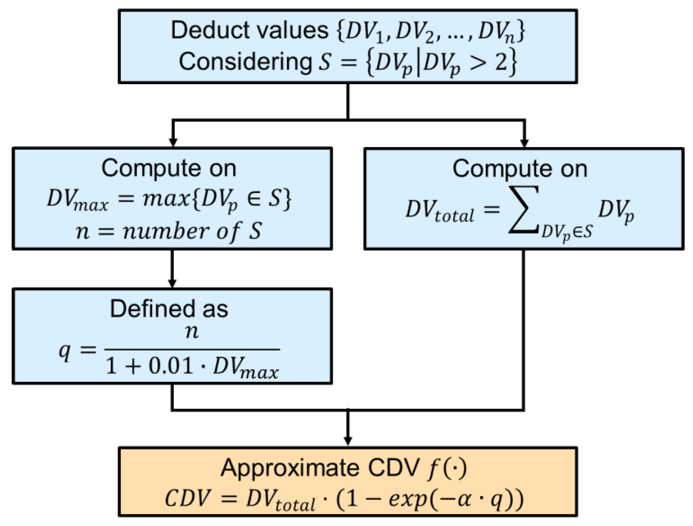
This formula fully expresses the mathematical relationship between the average PCI and the combinations of distresses within each block. The PCI deduction of each block depends not only on the number and severity of distresses but is also affected by the distribution patterns of distresses and their interactions, all of which can be dynamically adjusted through the function f(∙) in Figure 2. In the mathematical model for pavement condition assessment, the function f ( · ) serves as the critical core for determining the PCI value of each segment. It is responsible for aggregating and correcting the deduction values (Deduct Values, C m D U D ) of individual distress items within the segment, converting them into a single total deduction value—namely, the CDV as defined in ASTM D6433. This function must accurately reflect the overall damage level resulting from multiple distress types, varying severities, and affected areas, while considering the interactions between distresses to avoid misjudgment caused by simple summation. In this study, let the set of distresses for the k-th segment be defined as C m D U D 1 x m y m C m D U D S k , where each element represents the deduction value of a distress within the segment after accounting whether it has been repaired through resurfacing ( x m ) or localized repair ( y m ). The input to the function f ( · ) is then defined as the set of all deduction values { D V 1 , D V 2 , , D V n } corresponding to the distresses belonging to that segment. In the actual PCI calculation process, to avoid small defects from disproportionately affecting the results, only deduction values greater than 2 are considered. This yields the set S = { D V p | D V p > 2 } . Additionally, the maximum deduction value in this set is defined as D V m a x = m a x { D V p S } . According to the ASTM D6433 specification, the uncorrected total deduct value is first calculated as D V t o t a l = D V p S D V p . This value serves only as an intermediate variable and cannot be directly used to compute the PCI because multiple distresses may interact. Direct summation would lead to biased assessment results. Therefore, this study introduces an interaction parameter q, defined as q = n u m b e r   o f   S 1 + 0.01 · D V m a x . This formula reflects the trade-off between the number of distress items and the dominant distress (i.e., the largest DV) in the segment. When there are many distresses but no single one has a large impact, the CDV adjustment tends to be “moderate”; conversely, when a dominant distress exists, its influence is reinforced. The function f ( · ) essentially derives the final Corrected Deduct Value (CDV) from the two quantities D V t o t a l and q. In the ASTM standard, the CDV is obtained through lookup tables and graphical curves. However, for the purposes of mathematical modeling and automated computation, an exponential fitting model can be used to approximate the correction effect. A commonly used mathematical approximation is expressed as follows:
f D V 1 ,   D V 2 ,   ,   D V n = C D V = D V t o t a l ( 1 e x p ( α · q ) )
Among them, α is an empirical adjustment parameter, usually taking values in the range of 0.1 to 0.25, used to fit the characteristics of the ASTM correction curve. The meaning expressed by this formula is the following: the CDV approaches the total deduct value D V t o t a l , but exhibits a “slowly increasing saturation” trend constrained by the number of distresses and the strength of the principal distress (through the effect of q).
In addition, x m and y m are binary variables, respectively, indicating whether the m-th distress undergoes resurfacing maintenance and local maintenance. x m = 1 indicates that the m-th distress chooses resurfacing maintenance, and x m = 0 indicates that the m-th distress does not undergo resurfacing maintenance. y m = 1 indicates that the m-th distress chooses local maintenance, and y m = 0 means that the m-th distress does not undergo local maintenance. When x m = 0 and y m = 0 , it indicates that the m-th distress undergoes neither resurfacing maintenance nor local maintenance. This is an untreated situation, which should bear the deduction value of that distress; therefore, this term equals 1. When x m = 1 , it indicates that the m-th distress has chosen resurfacing maintenance, then 1 x m y m = 0 indicates that the distress is repaired with no deduction. When y m = 1 , it indicates that the m-th distress has chosen local maintenance, then 1 x m y m = 0 , indicating that the distress is locally repaired with no deduction. In this way, 1 x m y m in the objective function makes it so that only untreated distresses (i.e., distresses that have not undergone resurfacing or local maintenance) will have deductions and will be included in the calculation of the PCI value. C m D U D is the deduction value of the m-th distress, indicating the deduction incurred if the m-th distress does not receive appropriate maintenance. In the objective function, the deduction value C m D U D is multiplied by 1 x m y m , thus allowing the deduction to be adjusted according to whether resurfacing or local maintenance has been carried out. If the distress is not repaired (i.e., x m = 0 and y m = 0 ), then the deduction value C m D U D is added to the total deduction. If the distress is repaired (i.e., x m = 1 and y m = 1 ), then the distress no longer causes a deduction; thus, C m D U D × 0 = 0, which will not affect the total deduction. Therefore, the model will preferentially choose to repair these distresses (whether resurfacing or local maintenance) so as to maximize the average PCI.

2.2.3. Constraints

This section provides a detailed explanation of each constraint, which ensures the feasibility of the model and guides how to make reasonable decisions in terms of budget, resurfacing segments, maintenance methods, and so on. The purpose of designing these constraints is to ensure the feasibility, rationality, and financial viability of the model; the constraint conditions of this study are as follows: (1) non-overlapping resurfacing segment constraint: to avoid duplicate resource waste and ensure the uniqueness of each resurfacing segment. (2) Constraint on marking all distresses within resurfacing segments: to ensure that each distress is reasonably handled within the resurfacing segment. (3) Constraint of a unique maintenance method for a distress: to avoid a distress simultaneously choosing resurfacing and local maintenance, ensuring the uniqueness of the decision. (4) Budget constraint: to ensure that the total maintenance cost does not exceed the budget, ensuring financial feasibility. These constraints work together to ensure that the optimization model, within the budget and without wasting resources, selects the most appropriate maintenance strategy; the following will, in order, explain the contents of these constraints. Non-overlapping resurfacing sections constraint: prevents redundant resource usage and ensures the uniqueness of each resurfacing section.
A. 
Non-overlapping constraint of resurfacing segments
This constraint ensures that when selecting resurfacing segments, no two segments overlap each other. That is to say, once a certain segment is selected for resurfacing maintenance, other segments cannot overlap with it. This can avoid the waste of resurfacing resources and also make the maintenance plan more feasible.
s i , j + s i , j 1 , i , j i , j , m a x i , i < m i n j , j
If a certain segment i , j is selected as a resurfacing segment, i.e., s i , j = 1 , then all other segments i , j that overlap with it must be chosen not to resurface, i.e., s i , j = 0 . The definition for overlapping segments is that if m a x i , i < m i n j , j , it indicates that segments i , j and i , j overlap each other, and therefore they cannot be selected simultaneously. The purpose is to ensure the uniqueness and effectiveness of the selection of resurfacing segments, avoiding resource waste caused by multiple resurfacing segments. The selection of resurfacing segments is illustrated in Figure 3.
s i , j is a binary variable of 0 or 1, indicating whether to choose the segment from meter i to meter j to carry out “resurfacing maintenance”. When s i , j = 1 , it means that the segment will be fully resurfaced. Suppose meters 1 to 3 of the road are a resurfacing segment, i.e., s 1,2 = 1 . Then, other resurfacing segments s i , j must not overlap with s 1,2 , so it is necessary to impose non-overlapping conditions: (1) overlap at the start point of resurfacing segments; (2) overlap at the end point of resurfacing segments; and (3) partial overlap of resurfacing segments. As shown in Figure 3a, there is overlap at the start point of the resurfacing segment: the resurfacing segment s 2,3 overlaps with s 1,2 , and the start point of s 2,3 is at meter 2, which lies within s 1,2 ; hence, start point overlap occurs. Figure 3b shows overlap at the end point of the resurfacing segment: the resurfacing segment s 0,1 overlaps with s 1,2 , and the end point of s 0,1 is at meter 1, which lies within s 1,2 ; hence. end point overlap occurs. Figure 3c shows partial overlap of the resurfacing segment: the resurfacing segment s 0,3 overlaps with s 1,2 , and s 0,3 already contains s 1,3 ; hence, partial segment overlap occurs.
B. 
Constraint on marking all distresses within resurfacing segments
This constraint ensures that if a distress is located within a certain resurfacing segment, then that distress must choose resurfacing maintenance (i.e., x m = 1 ). At the same time, if a certain distress is not repaired by resurfacing (i.e., x m = 0 ), then its corresponding segment will not be selected for resurfacing.
i , j i C m L O C j s i , j = x m , m = 1,2 , , M
The coverage requirement of resurfacing segments is that if the m-th distress C m L O C is located within the interval i , j , i.e., i C m L O C j , then the corresponding resurfacing segment s i , j must be 1, and x m must also be 1, indicating that this distress must choose resurfacing maintenance. The purpose is to ensure the matching between the distress and the resurfacing segment, avoiding distresses within the segment not being properly repaired. If a distress falls within a certain segment, then that distress must undergo resurfacing maintenance.
C. 
Constraint of a unique maintenance method for a distress
This constraint ensures that each distress at most can only choose one maintenance method, that is, each distress either chooses resurfacing maintenance or chooses local maintenance, and cannot choose two methods simultaneously.
x m + y m 1 , m = 1,2 , , M
The single-selection rule is that each distress m can only choose one maintenance method. If x m = 1 , it indicates that the distress chooses resurfacing maintenance, then y m = 0 ; if y m = 1 , it indicates that the distress chooses local maintenance, then x m = 0 . The purpose is to avoid choosing two maintenance methods simultaneously, thereby ensuring the uniqueness of the maintenance strategy for each distress point.
D. 
Budget constraint
This constraint ensures that the total cost of resurfacing and local maintenance does not exceed the available total budget B.
0 i j L s i , j · j i · R + m = 1 M y m · C m C O S T B
The calculation of resurfacing cost: the cost of each resurfacing segment is given by its length (j − i) multiplied by the resurfacing cost per meter R, and whether that segment is chosen for resurfacing is determined by s i , j . The calculation of local maintenance cost: the cost of each local maintenance is determined by multiplying the repair cost of that distress C m C O S T by y m ; if that distress chooses local maintenance, then that cost is included. The purpose is to ensure that the total expenses of all selected resurfacing and local maintenance do not exceed the budget B, thereby making the maintenance plan financially feasible.

2.3. Genetic Algorithm Design

This study considers a combinatorial optimization problem for road pavement maintenance, in which for each pavement distress point, one may choose local patching or resurface the entire segment that covers that distress point. The objective is to maximize repair effectiveness under a limited budget (or equivalently minimize the number of unrepaired distress points), while avoiding decision conflicts (for example, overlapping resurfacing segments are not allowed). This type of problem can be modeled as integer programming, and this study seeks to design a genetic algorithm (GA) to solve it. The following explains in detail, from four aspects—chromosome encoding, fitness function, genetic operator design, and complete procedure—the way the GA is applied, supplemented with a simple example. In related applications in recent years, a GA has been widely applied to problems of complex transportation networks and pavement maintenance strategy selection; for example, Cheng & Che (2024) [23] in urban traffic management combined multiple objectives and environmental constraints, and also proposed a similar binary bit-encoding framework. And the systematic review by Kim, Park, and Shin (2022) [28] pointed out that a GA, in handling nonlinear structures involving segment selection and matching of maintenance types, possesses higher solving efficiency and global search capability relative to other methods. Therefore, the GA encoding and penalty-type fitness function designed in this study constitute a solution that conforms to academic logic and engineering practice in the current field.

2.3.1. Chromosome Encoding Design

A GA chromosome needs to fully represent the decision combination of which sections are resurfaced and which distress points are locally repaired. At the same time, the encoding must avoid infeasible situations (such as overlapping resurfacing sections). In this study, a simple and straightforward encoding approach is adopted, where decisions are converted into a fixed-length bit string. All candidate maintenance actions can be enumerated and represented with 0/1 to indicate whether the action is selected.
For example, suppose the roadway includes several predefined resurfacing sections and localized repair options for each distress point. One part of the chromosome corresponds to resurfacing decisions (1 indicates resurfacing the section, 0 indicates not resurfacing), while another part corresponds to localized repair decisions (1 indicates repairing the distress point, 0 indicates not repairing). This encoding is intuitive and facilitates the implementation of crossover and mutation.
However, overlapping sections require special handling: if two resurfacing sections overlap (covering part of the same roadway), they cannot be selected simultaneously in a single solution. To avoid such conflicts, infeasible combinations can be prevented during encoding (e.g., by excluding overlapping choices when generating initial solutions and performing genetic operations) or penalized heavily during fitness evaluation, making such chromosomes unlikely to be selected.
Additionally, this study applies constraint checking after generating or mutating chromosomes. If two overlapping sections are selected simultaneously, one of them can be randomly deselected, or the solution can be directly marked as infeasible with an extremely low fitness value.
An example of an encoding is as shown in Figure 4; suppose a road has 5 distress points (numbered 1 to 5, distributed sequentially along the road), and there are two possible resurfacing segments: Segment A covers distress points 1 and 2, and Segment B covers distress points 3 to 5. The chromosome can be represented by a bit string of length 7: the first two bits, respectively, represent whether to select resurfacing A and resurfacing B, and the last five bits, respectively, represent whether to perform single-point patching for distress points 1 to 5. For example, the chromosome 10|00110 can be interpreted as selecting resurfacing segment A (because the first bit = 1) but not selecting B (the second bit = 0); no local patching is needed for distress point 1 (because A already covers it). Since A covers points 1 and 2, single-point patching is therefore not performed, local patching is performed for points 3 and 4, and point 5 is not patched. Under feasible situations, if segment A is selected, then the local patching genes for points 1 and 2 should be regarded as invalid or forced to 0 in order to avoid duplicate maintenance. Similarly, if segments A and B are defined to overlap (there is no overlap in this example), they cannot be selected simultaneously. This study will ensure through the above mechanisms that the maintenance decision set corresponding to the chromosome is consistent and conflict-free. In the case study, the following GA parameter settings are adopted: the chromosome length is 7 bits (2 bits for resurfacing decisions and 5 bits for localized repair), the population size is 100, the crossover rate is 0.8, the mutation rate is 0.05, and the maximum number of generations is 500. These values were determined through preliminary sensitivity analysis to balance solution quality and computational efficiency.

2.3.2. Fitness Function Design

This study designs a fitness function (fitness function) to evaluate the quality of each chromosome (solution). It is necessary to transform the actual objectives (e.g., maximizing repair effectiveness, complying with the budget constraint) into fitness values. This study’s approach is to use the increase in the PCI score (pavement condition index) as the benefit evaluation: resurfacing or patching will increase the PCI of each road section, and the fitness can be defined as the overall PCI gain. Whether directly counting the number of repaired points or the PCI increase, the core is to assess the degree to which the plan improves the road condition; the greater the improvement, the higher the fitness. The budget constraint is an important constraint of this problem, and combinations of maintenance actions exceeding the budget should be avoided. In the fitness function, a penalty function is used to handle constraints: if the total cost of the plan corresponding to a chromosome does not exceed the budget, then no points are deducted; if it exceeds the budget, the fitness is reduced according to the degree of overspending. The form of the penalty can be to reduce the fitness by a value proportional to the overspent amount, or directly set the fitness very low or even 0, forcing the GA to eliminate such infeasible plans. By adjusting the penalty strength, it is possible to balance “encouraging the repair of more distresses” and “strictly controlling the budget” during the search process. For example, the fitness function can be defined as follows:
F x = U x λ · m a x 0 ,   C o s t x B
Here, U(x) is the benefit of plan x (such as the number of repaired points or the sum of PCI increases), Cost(x) is the total cost, B is the budget limit, and λ is the penalty coefficient (ensuring that the fitness drops sharply when the budget is violated). In this way, as long as a plan exceeds the budget, even if it repairs many points, the penalty term will lower its fitness, prompting the GA to prefer plans within the budget. For example, suppose the total number of distress points = 5, and the decision decoded from a certain chromosome is as follows: resurface segment A (cost 50 ten thousand, repairing 2 distress points), perform local patching for another 2 distress points (each costing 10 ten thousand), and there is 1 minor distress point left unrepaired. The budget limit is assumed to be 60 ten thousand (B = 60). This plan repairs a total of 4 distress points (benefit U = 4), Cost = 50 + 10 + 10 = 70 ten thousand, exceeding the budget by 10 ten thousand. If the penalty coefficient λ = 1, then the fitness F = 4 − 1(70 − 60) = −6 (a negative fitness indicates severe overspending, and in actual implementation, the lower bound of fitness will be set to zero). Because the fitness is very low, the GA will consider this plan inferior. During the evolution process, plans with higher fitness (for example, plans that slightly reduce some maintenance to meet the budget) will be more likely to be selected. If there is another plan B whose cost is exactly 60 ten thousand and repairs 3 points (no overspending), then even though the number of repaired points is slightly fewer, its fitness F = 3 is clearly higher than plan A, and the GA will prefer plan B. After many generations of evolution, the fitness function guides the algorithm to converge toward solutions with high benefits and feasibility (not exceeding the budget).

3. Case Study

3.1. Data Sources

This case study explores the pavement damage conditions and maintenance methods for Gaotie SN road in Zhongli City, Taiwan (see Figure 5). This section is a four-lane road, with a length of 11.7 km, and each lane has a width of 3.5 m. The purpose of the study is to analyze the main types of damage on this section, the maintenance methods adopted and their costs, and to discuss how to carry out road maintenance effectively, extend the service life of the road, and enhance traffic safety. Section 1 of Gaotie SN road in Zhongli City has a total length of 11.7 km, includes two lanes in the forward direction and two lanes in the opposite direction, with a total of four lanes, and each lane has a width of 3.5 m. To assess the road condition, a damage survey was conducted, recording different types of pavement damage. The survey data include the damage location, type of damage, maintenance method, maintenance cost, and discovery method. In this case study, 20 representative pavement damage cases were selected, as shown in Table 2; these cases reflect the different types of damage on this section and their distribution. All damage was found by contractor inspections, indicating that regular pavement inspections are carried out in this area to identify problems in a timely manner and address them.
In this road section, the most common type of damage is rutting, which is mainly caused by the repeated passage of heavy vehicles. These rutting damages appear in multiple segments, and the corresponding maintenance methods are mainly local patching or shallow pothole filling; the repair cost ranges from USD 200 to USD 567, varying according to the extent of the damage and the maintenance method. Cracks are also a common type of damage, including longitudinal cracks and transverse cracks. These cracks usually appear on the surface layer of the pavement; if not repaired in time, they will lead to further structural damage. Most of these cracks are repaired through crack filling and local thin overlay, with generally lower maintenance costs, about USD 186 to USD 410. In addition, patching issues and potholes are also relatively common. Patching refers to areas in the pavement that were previously repaired but have problems again, requiring re-local rehabilitation or local thin overlay. For potholes, local rehabilitation is usually used to restore the structural integrity of the pavement, with higher maintenance costs, about USD 385 to USD 635. According to different types of pavement damage, different maintenance methods were adopted, as shown in Table 3. The main maintenance methods include local patching, local rehabilitation, shallow pothole filling, and local thin overlay. Local patching is usually used for small-scale cracks and damage; after cleaning the damaged area, asphalt or concrete is filled for repair. This maintenance method has a relatively low cost, usually about USD 550 to USD 1150 per square meter. Local rehabilitation is mainly used for moderate damage; during construction, it is necessary to lay a new asphalt layer or carry out a more thorough repair, with higher costs, usually between USD 950 and USD 1900. Shallow pothole filling is a repair method aimed at minor potholes or small-scale damage, with maintenance costs usually between USD 210 and USD 260. Local thin overlay is used for surface-layer cracks or slight wear, with the lowest cost, usually between USD 186 and USD 410. The differences in maintenance costs mainly come from the extent and depth of the damage and the chosen maintenance method. The cost data presented in the table were obtained from the official contractor quotations used by the Zhongli City Government in 2023 and were cross-verified with historical bidding documents. The study section mainly consists of asphalt concrete pavements, with an average service age of approximately 7–12 years, depending on the sub-section.
When the extent of pavement damage is large and cannot be effectively resolved through local patching or rehabilitation, it may be necessary to choose resurfacing as the repair plan. Resurfacing involves comprehensively renewing the surface layer of the entire road section and re-laying new asphalt or concrete. This method is suitable for areas where pavement damage is relatively concentrated and severe. Depending on the length of the road, the cost of resurfacing also varies. The following are the data on the lane length and resurfacing cost, as shown in Table 4; as the lane length increases, the cost of resurfacing shows a linear increase. When medium- and long-length road sections are severely damaged and cannot be effectively handled through local repairs, resurfacing is an effective long-term solution, although its initial cost is relatively high.
All damage was discovered by contractor patrol inspections. Regular patrol inspections are crucial for discovering pavement problems. These patrols are usually carried out in sections, and each road segment undergoes a detailed inspection to ensure that even minor damage can be discovered in a timely manner. During the inspection process, in addition to manual visual inspection, advanced pavement detection technologies may also be used, such as pavement scanners or sensors, so as to precisely detect cracks, potholes, and other potential problems. The case study of Section 1 of Gaotie SN road in Zhongli City demonstrates the common types of damage in the area’s road maintenance and their repair methods. Rutting, cracks, and potholes are the main pavement problems, and a variety of maintenance methods were adopted for these problems, such as local patching, local rehabilitation, shallow pothole filling, and local thin overlay. The maintenance costs range from USD 186 to USD 635, varying according to the type of damage and the maintenance method. When the extent of pavement damage is large and cannot be effectively repaired, resurfacing becomes a suitable option, especially in areas where damage is concentrated. The cost of resurfacing increases with the increase in the lane length, providing a long-term effective solution. These maintenance methods and costs reflect effective strategies for carrying out pavement maintenance on urban roads. Regular patrols and timely repairs can effectively extend the service life of the road, reduce maintenance costs, and improve driving safety. This case study provides valuable experience for road maintenance in other Taiwanese cities and offers useful references for future pavement repairs.

3.2. Scenario Analysis

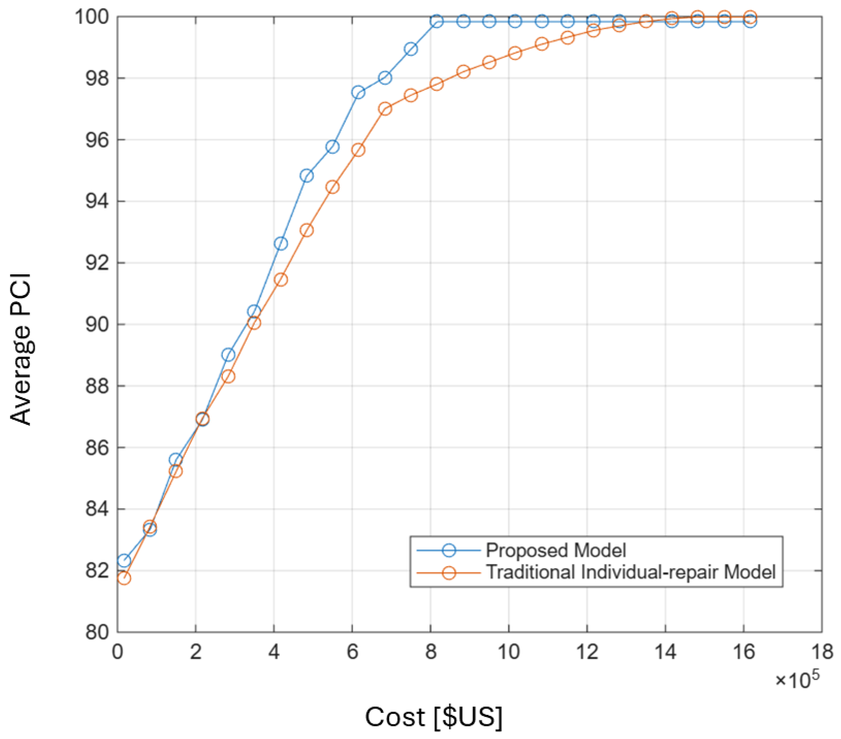
Compare the impact of two maintenance methods on the pavement condition index under different budget conditions and help decision-makers make more informed choices when planning road maintenance. As roads age and traffic volume increases, regular pavement maintenance becomes particularly important, and the rational allocation of maintenance budgets is key to ensuring long-term road operation and usage safety. According to the data shown in Table 5, the improvement effects on the pavement condition of two different maintenance methods under the same budget can be compared.
As the budget increases, whether it is “this method” or the “individual maintenance method,” both can significantly improve the pavement condition index, but the improvement effects differ. In a lower budget range, for example, when the budget is USD 20,000, the improvement effects of the two methods on the pavement condition are similar, with the average PCI reaching 82.5 and 82.2, respectively. This shows that when the budget is lower, the effects of the two methods are almost the same. However, as the budget increases, the gap begins to appear. When the budget increases to USD 80,000, the average PCI of “this method” rises to 83.7, while the PCI of the “individual maintenance method” also reaches 83.7, the two being equal; but within subsequent budget ranges, the gap gradually widens. When the budget reaches USD 280,000, the difference becomes more obvious. The average PCI of “this method” has increased to 91.1, while that of the “individual maintenance method” is 89.0, showing that “this method” has a more significant improvement effect under a higher budget. This trend becomes even more evident in higher budget ranges. When the budget reaches USD 1,550,000, the average PCI of “this method” reaches 100, while that of the “individual maintenance method” is 99.9, indicating that under a large budget situation, “this method” can more effectively improve the pavement condition to the optimal level. In summary, as shown in Figure 6, as the budget increases, the difference in effectiveness between the two methods becomes more pronounced. At a lower budget, the effects of the two are similar, but when the budget is higher, “this method” can significantly improve the pavement condition, whereas the “individual maintenance method” is relatively more stable. This indicates that, if one hopes to obtain the best pavement improvement effect under a high budget, “this method” is a more advantageous choice, whereas under a low budget, the effects of the two are close, and the “individual maintenance method” may be a more economical choice.
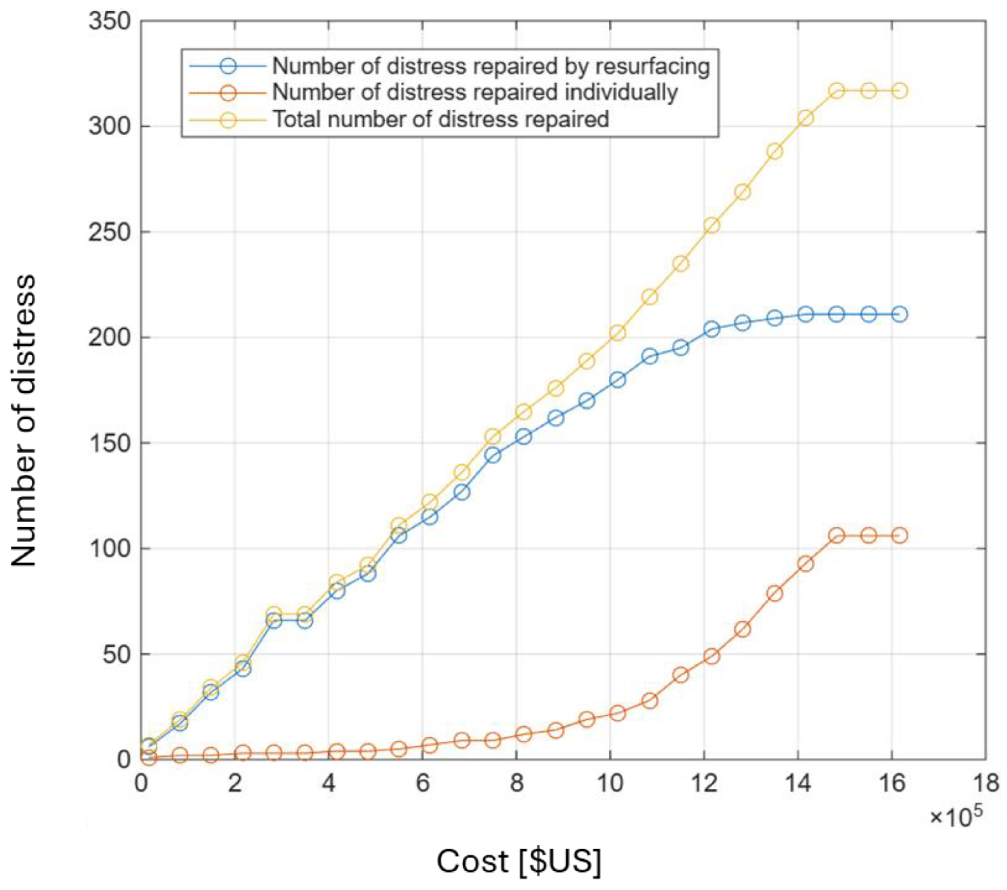
Under different budgets, the numbers of damages repaired corresponding to resurfacing and individual maintenance methods in the optimized maintenance strategy are as shown in Figure 7. It shows how the number of pavement damages handled by resurfacing and individual maintenance methods changes as the budget increases, and reveals the effectiveness of the optimized maintenance strategy under different budget conditions. Firstly, when the budget is relatively low, for example, USD 20,000, only six damages need to be repaired by resurfacing, and no individual maintenance is carried out. This shows that under a lower budget, choosing resurfacing can concentrate resources to handle fewer damaged areas. As the budget gradually increases, the number of damages handled by resurfacing also gradually rises. For example, with a budget of USD 80,000, the number of resurfacing repairs reaches 21, and under higher budgets (such as USD 350,000 or USD 480,000), the numbers of resurfacing repairs are 73 and 104, respectively, showing that under a higher budget, more damaged areas can be handled. On the other hand, individual maintenance is not activated when the budget is lower. As the budget gradually grows, especially above USD 150,000, the number of individual maintenance actions begins to increase. Taking USD 150,000 as an example, individual maintenance handled 1 damage, and when the budget further increased to USD 1,620,000, the number of damages handled by individual maintenance reached 92. This indicates that when the budget reaches a certain amount, in addition to resurfacing, more damages will be addressed through individual maintenance, further optimizing the maintenance strategy. In summary, as the budget increases, the numbers of resurfacing repairs and individual maintenance gradually rise. When the budget is lower, resurfacing is the main repair method, and as the budget increases, individual maintenance gradually becomes an important supplementary method to handle other damages that cannot be resolved through resurfacing. When the budget reaches the highest point, the numbers of both resurfacing and individual maintenance reach their maximum, indicating that with sufficient budget, the maintenance work will be comprehensively covered and achieve the best effect. These data reflect how, under an optimized maintenance strategy, to reasonably choose maintenance methods according to the budget, achieving the goal of both effectively improving pavement condition and reasonably allocating resources.
Under the optimized maintenance strategy, the situation of resurfacing segments is as shown in Table 6. These data provide detailed information on the number of pavement damages, average deduction values, and resurfacing lengths for different segments, helping this study understand the distribution of pavement damage and the scope where resurfacing is needed. Firstly, the table shows the resurfacing needs of multiple segments, whose numbers of damages range from small to large. For example, in the segment with start and end kilometer markers from 2 to 47 km, there are only three damages, and the resurfacing length is 45 m, indicating that the damage in this segment is relatively light and the maintenance demand is smaller. In other segments, such as 3801 to 4101 km, this segment has 18 damages, and the resurfacing length reaches 300 m, indicating that the damage in this segment is relatively concentrated and a larger area of resurfacing is needed to restore the pavement function. In addition, the average deduction value is an important indicator for measuring the degree of pavement damage. The table shows that some segments have higher deduction values; for example, the average deduction value of the 2 km to 47 km segment is 24.00, indicating that the damage in this segment is relatively severe and needs to be addressed in a timely manner. In other segments, such as 10,439 km to 10,466 km, the average deduction value of this segment is lower, at 2.75, showing that the damage in this segment is lighter and the need for resurfacing is relatively smaller. As the budget increases, the resurfacing length and the number of damages also gradually increase. Under higher budget conditions, the scope of the work expands, and larger-scale resurfacing will be carried out on segments where the damage is relatively concentrated. For example, in the 3801 km to 4101 km segment, because there are 18 damages and the resurfacing length is 300 m, it indicates that this segment needs large-scale resurfacing, because the damaged area in this segment is large and severe, and comprehensive repair must be carried out. These data help this study determine the maintenance priority of different segments and allocate resources reasonably according to factors such as the number of damages, deduction values, and resurfacing length. When the budget is limited, segments with more severe and larger-scale damage should be given priority, which can maximize maintenance efficiency and ensure driving safety. Relatively speaking, segments with lighter damage can be appropriately postponed, concentrating resources on the places that most urgently need repair. Overall, these data provide an effective reference to help this study carry out precise maintenance planning according to the specific pavement conditions, ensuring the efficiency and cost-effectiveness of road maintenance.

4. Conclusions

The motivation of this study arises from the maintenance challenges posed by uneven pavement distress distribution under limited budgets. By integrating MILP and a GA, this study proposes a multi-level framework that formalizes the logical mutual exclusivity between “resurfacing” and “localized patching.” Experimental analyses show that under medium-budget conditions, the proposed method can achieve an additional improvement of approximately 1.5–3.5 PCI points compared with traditional strategies, while maintaining cost efficiency. The results not only provide feasible resource allocation guidelines for road management agencies but also highlight the trade-off between repair coverage and pavement quality. This study combines mixed-integer linear programming and genetic algorithms, and, in response to the real-world conditions of uneven pavement distress distribution and limited resources, develops an optimized maintenance method that simultaneously covers two levels: “segment resurfacing” and “local patching at distress points.” Compared with individual maintenance approaches that rely only on fixed-length resurfacing or a single patching strategy, this method, through mathematical modeling of logical mutual exclusivity, precisely handles the choice relationship between the two maintenance approaches, avoids misplacement of resurfacing and overlapping waste of resources, and can still flexibly adjust the direction of resource deployment when the distress distribution differs significantly. The model is designed with high flexibility, allowing dynamic allocation of maintenance resources according to distress severity, spatial distribution, and budget constraints, while also supporting the inclusion of additional policy conditions, so that it can align with practical road maintenance needs. On the solution side, this study uses genetic algorithms to conduct heuristic search, overcoming the time bottleneck of individual maintenance mixed-integer programming when computing large-scale road networks, and obtaining near-optimal solutions within reasonable computation time. Case analyses show that under low-budget scenarios, this method performs comparably to individual maintenance point-by-point patching; however, as the budget increases, this method significantly outperforms individual maintenance approaches in terms of average PCI improvement magnitude, maintenance coverage rate, and resource utilization efficiency, and can raise the pavement condition to an optimal level in high-budget scenarios. In practical application, this method can provide road maintenance agencies with a data-based quantitative decision-making tool, replacing planning approaches that rely on experience and manual judgment, and ensuring that limited funds are invested in the maintenance plans with the highest benefits. Because the input data required by the model are highly compatible with existing pavement management systems, they can be directly integrated into current smart pavement management platforms to realize the datafication and systematization of decision-making. In sum, this study not only fills, at the theoretical level, the gaps in the existing literature regarding multi-level maintenance strategy modeling, but also provides, at the practical level, a decision-support solution with high efficiency, high accuracy, and extensibility; in the future, it can be further extended to multi-objective optimization and cross-year maintenance planning to enhance the sustainability and cost-effectiveness of infrastructure maintenance. In addition, combining the maintenance planning model with image recognition systems is expected to enhance the overall performance and real-time responsiveness of smart pavement management systems.

Author Contributions

Conceptualization, Y.-S.C.; methodology, Y.-S.C., P.-Y.S., J.-D.L., and C.-y.K.; investigation, Y.-S.C., S.-H.L., and P.-Y.S.; writing—original draft preparation, Y.-S.C.; writing—review and editing, M.-C.H. and J.-D.L.; supervision, Min-Che Ho and J.-D.L. All authors have read and agreed to the published version of the manuscript.

Funding

This research received no external funding.

Data Availability Statement

The data generated in this study are not publicly available due to commercial confidentiality and project-related restrictions.

Conflicts of Interest

The authors declare no conflicts of interest.

References

  1. Margorínová, M.; Trojanová, M.; Decký, M.; Remišová, E. Noise costs from road transport. Civ. Environ. Eng. 2018, 14, 12–20. [Google Scholar] [CrossRef]
  2. Fwa, T.F.; Chan, W.T.; Hoque, K.Z. Analysis of pavement management activities programming by genetic algorithms. Transp. Res. Rec. 1998, 1643, 1–6. [Google Scholar] [CrossRef]
  3. Elhadidy, A.A.; Elbeltagi, E.E.; Ammar, M.A. Optimum analysis of pavement maintenance using multi-objective genetic algorithms. HBRC J. 2015, 11, 107–113. [Google Scholar] [CrossRef]
  4. Santos, J.; Ferreira, A.; Flintsch, G. A multi-objective optimization approach for sustainable pavement management. Struct. Infrastruct. Eng. 2018, 14, 854–868. [Google Scholar] [CrossRef]
  5. Santos, J.; Ferreira, A.; Flintsch, G. An adaptive hybrid genetic algorithm for pavement management. Int. J. Pavement Eng. 2019, 20, 266–286. [Google Scholar] [CrossRef]
  6. Yamany, M.S.; Abraham, D.M.; Ventresca, M.; Nantung, T.; Labi, S. Probabilistic optimization of pavement preventive maintenance using multi-objective genetic algorithm. Innov. Infrastruct. Solut. 2025, 10, 194. [Google Scholar] [CrossRef]
  7. Yamany, M.S.; Cawley, L.; Reza, I.; Ksaibati, K. Network-level pavement maintenance and rehabilitation planning using genetic algorithm. Innov. Infrastruct. Solut. 2024, 9, 208. [Google Scholar] [CrossRef]
  8. Yang, C.; Remenyte-Prescott, R.; Andrews, J.D. Pavement maintenance scheduling using genetic algorithms. Int. J. Perform. Eng. 2015, 11, 135. [Google Scholar]
  9. Hamdi, H.; Hadiwardoyo, S.P.; Correia, A.G.; Pereira, P.A. Pavement maintenance optimization strategies for national road network in Indonesia applying genetic algorithm. Procedia Eng. 2017, 210, 253–260. [Google Scholar] [CrossRef]
  10. Wang, D.; Li, S.; Zhou, X. Preventive maintenance decision-making optimization method for airport runway composite pavements. Transp. Res. Rec. 2019, 2673, 227–237. [Google Scholar]
  11. Yang, B.; Luo, F. Integer search algorithm: A new discrete multi-objective algorithm for pavement maintenance management optimization. Expert Syst. Appl. 2020, 160, 113699. [Google Scholar]
  12. Feng, K.; Zhang, T.; Liu, M. Research on multi-Objective Pavement Maintenance Decision-Making Optimization Considering Uncertainty Factors. Master’s Thesis, Chang’an University, Xi’an, China, 2020. [Google Scholar]
  13. Shan, F.; Li, H.; Wang, Z.; Jin, M.; Chen, D. Optimizing rural highway maintenance scheme with mathematical programming. Appl. Sci. 2024, 14, 8253. [Google Scholar] [CrossRef]
  14. Guan, X.; Zhang, H.; Du, X.; Zhang, X.; Sun, M.; Bi, Y. Optimization for asphalt pavement maintenance plans at network level: Integrating maintenance funds, pavement performance, road users, and environment. Appl. Sci. 2023, 13, 8842. [Google Scholar] [CrossRef]
  15. Bo, W.; Zhang, Y.; Liu, J.; Chen, F.; Zhao, X. MILP-based approach for high-altitude region pavement maintenance decision optimization. Appl. Sci. 2024, 14, 7670. [Google Scholar] [CrossRef]
  16. Chen, Y.; Liu, Q.; Lin, T. A pavement crack detection and evaluation framework for a UAV inspection system based on deep learning. Autom. Constr. 2022, 138, 104273. [Google Scholar] [CrossRef]
  17. Zhao, H.; Wang, L.; Yu, P. A highway pavement crack identification method based on an improved U-Net model. J. Intell. Transp. Syst. 2021, 25, 525–537. [Google Scholar]
  18. Bruno, S.; Colonnese, S.; Scarano, G.; Del Serrone, G.; Loprencipe, G. Pavement distress estimation via signal on graph processing. Sensors 2022, 22, 9183. [Google Scholar] [CrossRef] [PubMed]
  19. Loprencipe, G.; Pantuso, A. A specified procedure for distress identification and assessment for urban road surfaces based on PCI. Coatings 2017, 7, 65. [Google Scholar] [CrossRef]
  20. New Taipei City Government. New Taipei City Smart Pavement Management Center and Road Maintenance Analysis; Municipal Infrastructure Report; New Taipei City Government: New Taipei City, China, 2023.
  21. Sun, W.; Lin, C.; Hou, J. Using an airport pavement management system to optimize the influence of maintenance alternatives on operating conditions. J. Transp. Eng. Part B Pavements 2018, 144, 04018017. [Google Scholar]
  22. Zhang, P.; Yi, W.; Song, Y.; Gao, Y.; Wu, P. Optimizing large-scale road maintenance plan in Western Australia. SSRN 2024, preprint. [Google Scholar]
  23. Cheng, X.; Che, C. Optimizing urban road networks for resilience using genetic algorithms. Acad. J. Sociol. Manag. 2024, 2, 1–7. [Google Scholar]
  24. Fard, A.; Yuan, A.X.X. Multi-year maintenance planning for large-scale infrastructure systems: A novel network deep Q-learning approach. arXiv 2025, arXiv:2507.18732. [Google Scholar]
  25. Indriastiwi, F.; Hadiwardoyo, S.P. Optimizing multimodal infrastructure development in Java: A budget-constrained planning approach. Civ. Eng. Archit. 2025, 13, 2735–2749. [Google Scholar] [CrossRef]
  26. Asadifakhr, K.; Roy, S.; Han, F.; Bell, E. Flowing together: Synergistic road-stream crossing replacement prioritization for balanced stakeholder interests. In Proceedings of the AGU Fall Meeting 2024, Washington, DC, USA, 9–13 December 2024. [Google Scholar]
  27. ASTM D6433-18; Standard Practice for Roads and Parking Lots Pavement Condition Index Surveys. ASTM International: West Conshohocken, PA, USA, 2018.
  28. Kim, H.; Park, J.; Shin, Y. Pavement maintenance decision making based on optimization models. J. Infrastruct. Syst. 2022, 28, 04022025. [Google Scholar]
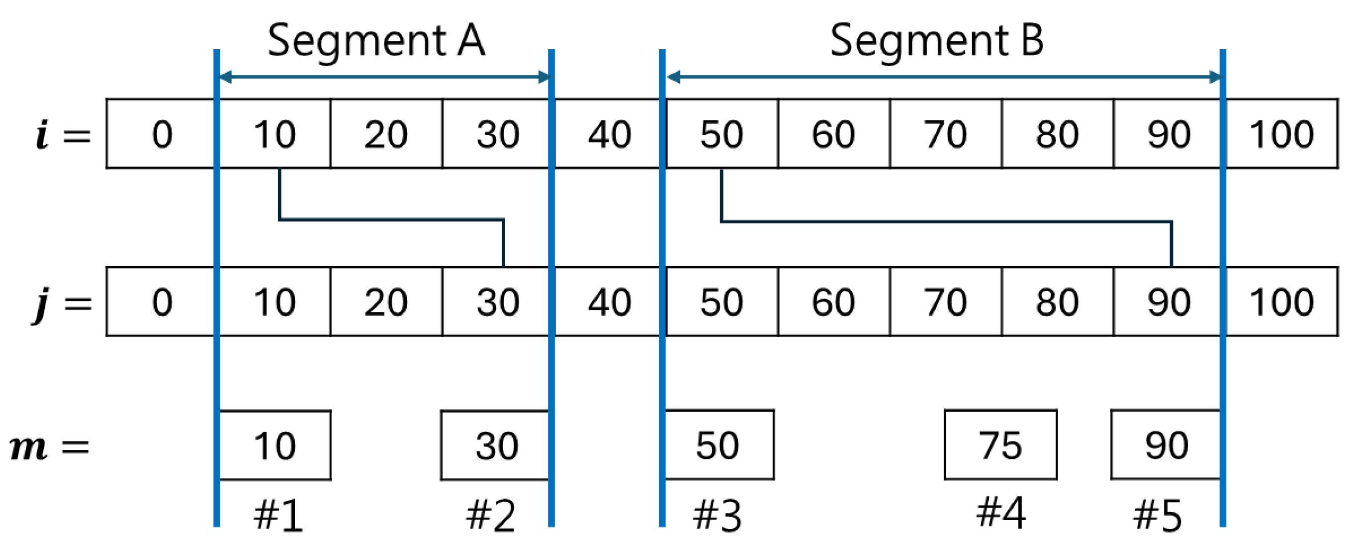
Figure 1. Road maintenance decision scenario.
Applsci 15 10094 g001
Figure 2. CDV estimation procedure.
Applsci 15 10094 g002
Figure 3. Example of the constraint condition to avoid overlapping of resurfacing segments. The resurfacing start and end points cannot contain the following non-overlapping conditions: (a) overlap at the start point of the resurfacing segment; (b) overlap at the end point of the resurfacing segment; and (c) partial overlap of the resurfacing segment.
Applsci 15 10094 g003
Figure 4. Genetic algorithm encoding example explanation.
Applsci 15 10094 g004
Figure 5. Road section used in the case study (highlighted in red).
Applsci 15 10094 g005
Figure 6. Distribution of average PCI under different budgets.
Applsci 15 10094 g006
Figure 7. Distribution results of the number of pavement damage repairs under different budgets.
Applsci 15 10094 g007
Table 1. List of parameters and variables used by the model.
SymbolsExplanation
m Distress point index, m = 1,2 , 3 , , M .
i , j Resurfacing segment index, satisfying 0 ≤ i ≤ j ≤ L.
L Total road length (meters).
M Total number of distresses.
C m L O C The location of the m-th distress, in meters, indicating the specific location of the m-th distress on the road.
C m D U D The deduction value of the m-th distress, indicating the deduction incurred if that distress is not properly repaired.
C m C O S T The repair cost of the m-th distress, expressed in monetary units, indicating the cost to repair that distress.
R The cost of resurfacing maintenance per meter, indicating the cost required to repair 1 m of road.
B The total maintenance budget, indicating the total amount of available funds in all maintenance activities.
s i , j If the road segment from meter i to meter j undergoes resurfacing maintenance, then it is 1, otherwise it is 0.
x m If the m-th distress is repaired by resurfacing, then it is 1, otherwise it is 0.
y m If the m-th distress is repaired by local maintenance, then it is 1, otherwise it is 0.
Table 2. Damage survey list of the studied road, only the first 20 records are listed.
IDLocationTypeMethodCost (USD)Discovery
13K+772RuttingLocal rehabilitation454Contractor patrol inspection
210K+529Alligator crackingShallow pothole filling210Contractor patrol inspection
39K+728RuttingLocal patching567Contractor patrol inspection
41K+324Longitudinal and transverse cracksLocal thin overlay186Contractor patrol inspection
57K+212PatchingLocal rehabilitation435Contractor patrol inspection
63K+595PatchingLocal thin overlay163Contractor patrol inspection
77K+595RuttingShallow pothole filling260Contractor patrol inspection
81K+107PatchingLocal rehabilitation589Contractor patrol inspection
910K+692PotholesLocal rehabilitation635Contractor patrol inspection
105K+349PatchingShallow pothole filling366Contractor patrol inspection
1111K+516Alligator crackingLocal rehabilitation410Contractor patrol inspection
123K+675PotholesLocal rehabilitation385Contractor patrol inspection
132K+648RuttingLocal patching517Contractor patrol inspection
146K+479RuttingShallow pothole filling210Contractor patrol inspection
158K+295Longitudinal and transverse cracksLocal patching367Contractor patrol inspection
166K+918PatchingLocal thin overlay199Contractor patrol inspection
1711K+183PatchingLocal patching594Contractor patrol inspection
185K+903RuttingLocal patching436Contractor patrol inspection
199K+296PatchingLocal patching564Contractor patrol inspection
2010K+132RuttingShallow pothole filling200Contractor patrol inspection
Table 3. List of road damage maintenance methods.
Maintenance MethodApplicable SituationConstruction MethodCost per Square Meter (USD)
Shallow pothole fillingRepair small-area and shallow potholes on the pavement.Clean the pothole area, remove loose material or debris, then fill with appropriate repair material.200~400
Local patchingA repair method for small-scale pavement damage, particularly suitable for cracks, potholes, or other local damage.Clean the damaged area, remove loose material, then fill with repair materials such as asphalt or concrete, and compact.300~600
Local rehabilitationRepair pavement with larger-area or moderate-severity damage.Lay a new layer of asphalt on the original pavement surface layer, and compact.350~700
Local thin overlayApplicable to situations where the pavement surface layer has slight wear, aging, or slight cracks.Evenly apply asphalt emulsion on the original pavement surface, then spread crushed stone or aggregate, and compact.100~200
Table 4. List of road resurfacing costs.
Lane Length (Meters)Resurfacing Cost (USD)
56400
107700
159033
2010,267
2511,333
3012,567
3515,733
4017,000
4518,233
5019,467
10031,000
15043,333
20056,000
25068,000
30080,333
35093,333
Table 5. Results of average PCI improvement under different budgets for maintenance optimization strategy.
Budget (USD)Average PCI of MethodAverage PCI of Individual Maintenance Method
USD 20,00082.5282.21
USD 80,00083.7483.74
USD 150,00087.0085.65
USD 220,00088.8087.35
USD 280,00091.1388.99
USD 350,00092.6690.31
USD 420,00093.6691.80
USD 480,00094.8093.12
USD 550,00096.4394.17
USD 620,00097.5395.40
USD 680,00098.6796.92
USD 750,00099.3197.41
USD 820,000100.0097.78
USD 880,000100.0098.09
USD 950,000100.0098.40
USD 1,020,000100.0098.71
USD 1,080,000100.0098.95
USD 1,150,000100.0099.16
USD 1,220,000100.0099.40
USD 1,280,000100.0099.55
USD 1,350,000100.0099.71
USD 1,420,000100.0099.82
USD 1,480,000100.0099.92
USD 1,550,000100.00100.00
USD 1,620,000100.00100.00
Table 6. List of optimized resurfacing segments (first 20 entries).
Start
(Meters)
End
(Meters)
Number of
Distresses
Average
Deduction Value
Resurfacing Length
(Meters)
247324.0045
819634.3315
15317324.5020
199224213.0025
454489320.6735
608618121.0010
74374815.005
764864713.86100
92494934.3325
10181043227.5025
14631513511.8050
162817781015.50150
18471877222.0030
19231928125.005
20492089324.3340
21762181137.005
22942444814.38150
26082623218.5015
29553000320.0045
32273257312.0030
Disclaimer/Publisher’s Note: The statements, opinions and data contained in all publications are solely those of the individual author(s) and contributor(s) and not of MDPI and/or the editor(s). MDPI and/or the editor(s) disclaim responsibility for any injury to people or property resulting from any ideas, methods, instructions or products referred to in the content.