Author Contributions
Conceptualization, D.E.-O., B.C.-F., P.P.-C., A.V., L.Z.-V., D.A.-G., L.R.-C., A.T.-E., C.C.-M., F.V.-M., C.G. and P.A.-V.; methodology, D.E.-O., B.C.-F., P.P.-C., A.V., L.Z.-V., D.A.-G., L.R.-C., A.T.-E., C.C.-M., F.V.-M., C.G. and P.A.-V.; software, D.E.-O., B.C.-F., P.P.-C., A.V., L.Z.-V., D.A.-G., L.R.-C., A.T.-E., C.C.-M., F.V.-M., C.G. and P.A.-V.; validation, D.E.-O., B.C.-F., P.P.-C., A.V., L.Z.-V., D.A.-G., L.R.-C., A.T.-E., C.C.-M., F.V.-M., C.G. and P.A.-V.; formal analysis, D.E.-O., B.C.-F., P.P.-C., A.V., L.Z.-V., D.A.-G., L.R.-C., A.T.-E., C.C.-M., F.V.-M., C.G. and P.A.-V.; investigation, D.E.-O., B.C.-F., P.P.-C., A.V., L.Z.-V., D.A.-G., L.R.-C., A.T.-E., C.C.-M., F.V.-M., C.G. and P.A.-V.; resources, D.E.-O., B.C.-F., P.P.-C., A.V., L.Z.-V., D.A.-G., L.R.-C., A.T.-E., C.C.-M., F.V.-M., C.G. and P.A.-V.; Data curation, D.E.-O., B.C.-F., P.P.-C., A.V., L.Z.-V., D.A.-G., L.R.-C., A.T.-E., C.C.-M., F.V.-M., C.G. and P.A.-V.; writing—original draft, D.E.-O., B.C.-F., P.P.-C., A.V., L.Z.-V., D.A.-G., L.R.-C., A.T.-E., C.C.-M., F.V.-M., C.G. and P.A.-V.; writing—review & editing, D.E.-O., B.C.-F., P.P.-C., A.V., L.Z.-V., D.A.-G., L.R.-C., A.T.-E., C.C.-M., F.V.-M., C.G. and P.A.-V.; visualization, D.E.-O., B.C.-F., P.P.-C., A.V., L.Z.-V., D.A.-G., L.R.-C., A.T.-E., C.C.-M., F.V.-M., C.G. and P.A.-V.; supervision, D.E.-O., D.A.-G., A.T.-E., C.C.-M., F.V.-M. and C.G.; project administration, D.A.-G. and F.V.-M.; funding acquisition, C.G. and P.A.-V. All authors have read and agreed to the published version of the manuscript.
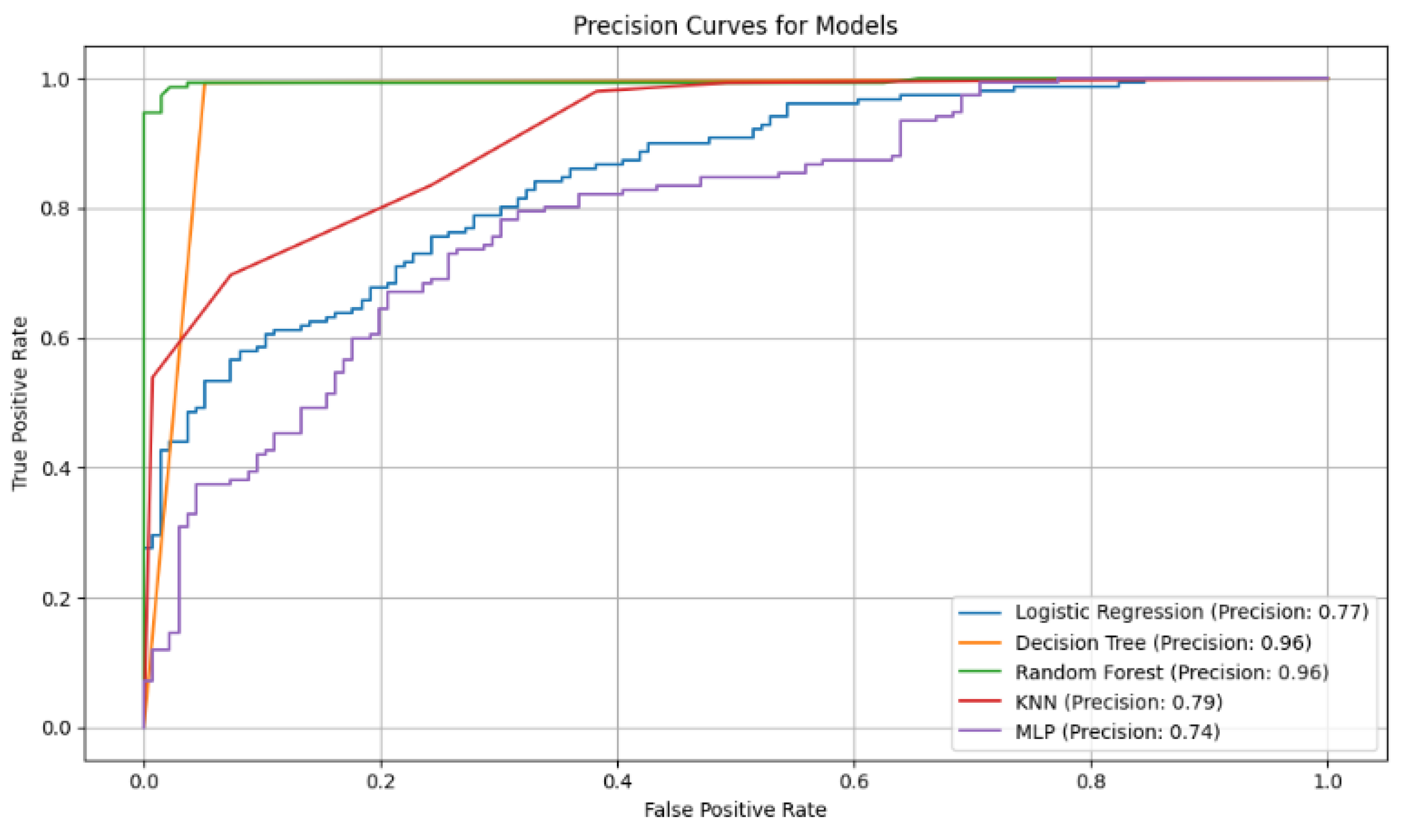
Figure 2.
Accuracy curves for the five classification models with selected variables. The Random Forest curve shows higher accuracy in correctly identifying positive cases, highlighting its robustness compared to other models evaluated.
Figure 2.
Accuracy curves for the five classification models with selected variables. The Random Forest curve shows higher accuracy in correctly identifying positive cases, highlighting its robustness compared to other models evaluated.
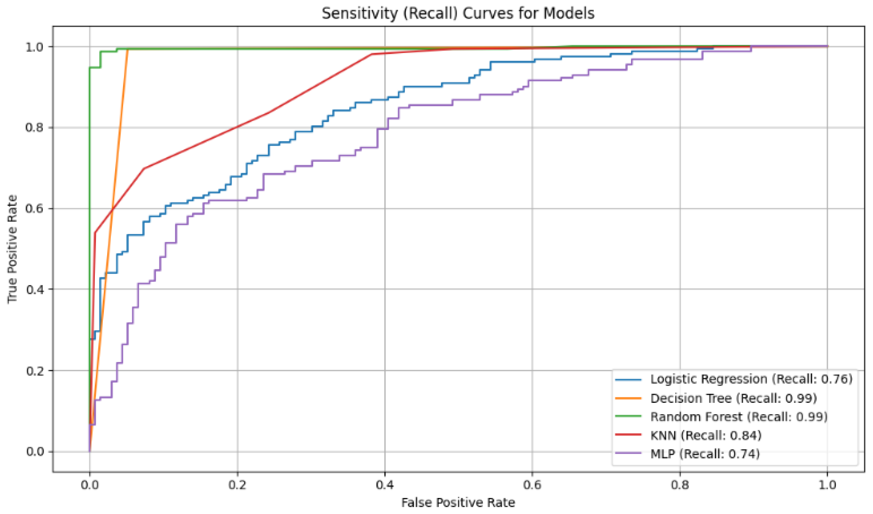
Figure 3.
Analysis of Sensitivity (Recall): This metric evaluates a model’s ability to find all positive cases.
Figure 3.
Analysis of Sensitivity (Recall): This metric evaluates a model’s ability to find all positive cases.
Figure 4.
Analysis of Specificity: It measures a model’s ability to correctly identify negative cases.
Figure 4.
Analysis of Specificity: It measures a model’s ability to correctly identify negative cases.
Figure 5.
Analysis of Balance (F1-Score): This score represents the harmonic mean between precision and sensitivity.
Figure 5.
Analysis of Balance (F1-Score): This score represents the harmonic mean between precision and sensitivity.
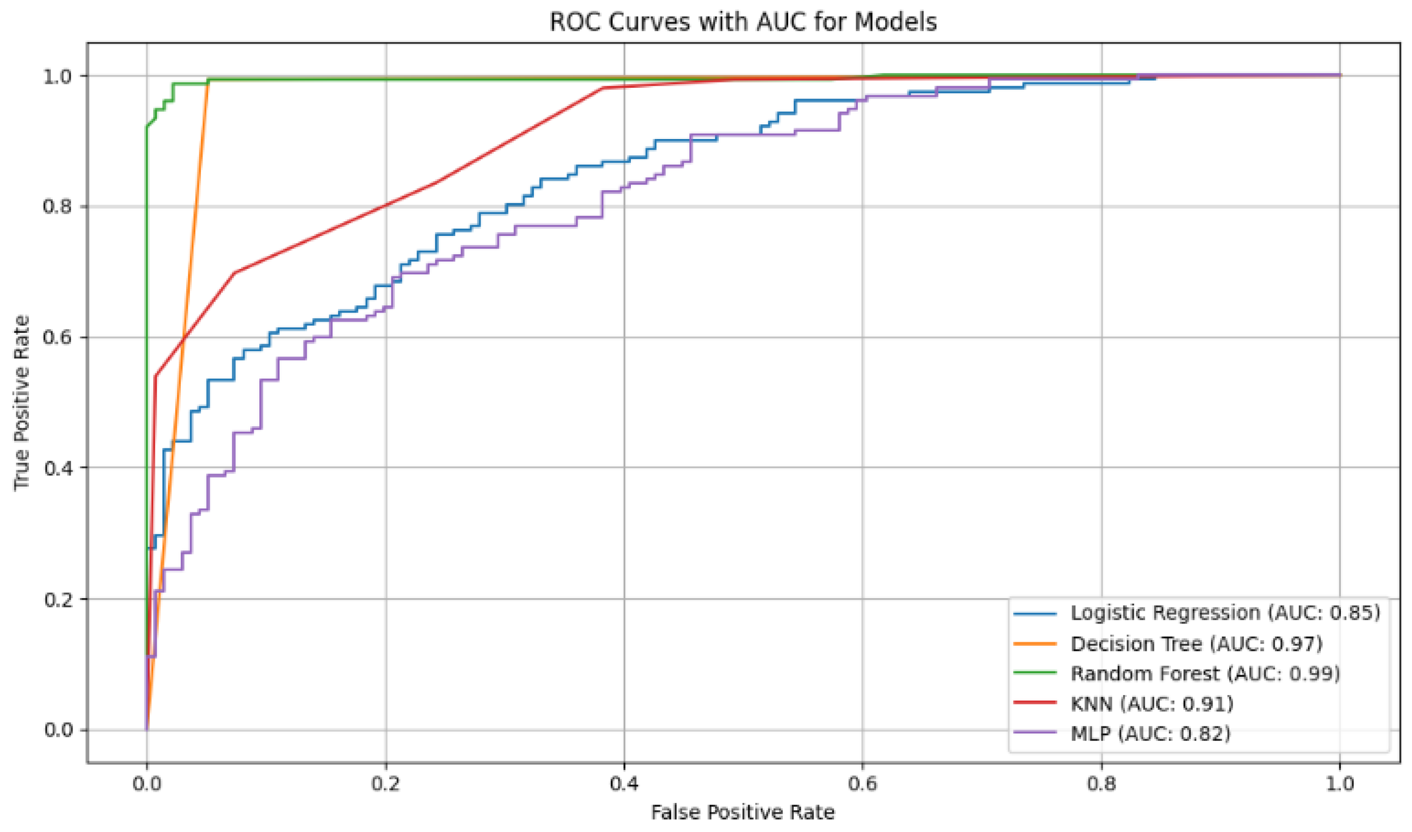
Figure 6.
ROC curves with AUC values for the diabetes classification models. The curves show that Random Forest (AUC = 0.99) and Decision Tree (AUC = 0.97) have the best discriminatory ability to differentiate between diabetic and non-diabetic patients.
Figure 6.
ROC curves with AUC values for the diabetes classification models. The curves show that Random Forest (AUC = 0.99) and Decision Tree (AUC = 0.97) have the best discriminatory ability to differentiate between diabetic and non-diabetic patients.
Table 1.
Comparative of machine learning studies for diabetes prediction.
Table 1.
Comparative of machine learning studies for diabetes prediction.
| Description | P. Languages | Model | Precision | Recall | F1 Score | Cite |
|---|
| An automatic diabetes prediction was developed using the Pima Indian dataset and a private database of 203 women. | Python | LG | 78% | 77% | 77% | [22] |
| KNN | 78.43% | 76.37% | 76% |
| RF | 78.45% | 78.13% | 78.28% |
| DT | 75.25% | 73.56% | 73% |
| Bagging | 80.15% | 79.25% | 79.23% |
| Adaboost | 79.56% | 78.45% | 78.12% |
| This study proposes a fused machine learning model, using a database of 768 women in the age range of 21 years. | Python | MLP | 95% | - | - | [24] |
| Three diabetes prediction models were evaluated using a dataset with 1879 samples and 46 variables. | - | LR | 85.70% | 81.20% | 82.90% | [29] |
| Random Forest | 93.70% | 93.80% | 94.80% |
| BPNN | 79.70% | 78.80% | 78.50% |
| Presents a diagnosis of Diabetes at Sylhet Diabetes Hospital (Bangladesh), 520 patients. | Python | LR | 95.46% | 98.56% | 96% | [30] |
| RF | 98.56% | 98.23% | 99.13% |
| Decision tree | 95.45% | 98.56% | 96.35% |
| SVM | 95.34% | 98.67% | 96.52% |
Table 2.
Dataset attributes used for diabetes prediction.
Table 2.
Dataset attributes used for diabetes prediction.
| Attribute | Variable Type | Units | Description |
|---|
| Pregnancies | Integer | None | Number of pregnancies |
| Glucose | Integer | mg/dL | Blood glucose level |
| BloodPressure | Integer | mmHg | Diastolic blood pressure |
| Skin Thickness | Integer | mm | Triceps skinfold thickness |
| Insulin | Integer | U/mL | Insulin level |
| BMI | Float | kg/m2 | Body Mass Index |
| DiabetesPedigree | Float | None | Diabetes risk based on family history |
| Age | Integer | Years | Age of the individual |
| Outcome | Binary | None | Presence (1) or absence (0) of diabetes |
Table 3.
Hyperparameter configuration for the models used.
Table 3.
Hyperparameter configuration for the models used.
| Model | Hyperparameter | Value Used | Justification | Reference |
|---|
| Logistic Regression | penalty | l2 | Prevents overfitting with L2 regularization. | [35] |
| C | 1.0 | Standard value for balancing fit and complexity. | |
| solver | lbfgs | An efficient and widely used optimizer. | |
| max_iter | 1000 | Ensures the optimization algorithm converges. | |
| Decision Tree | criterion | gini | Computationally efficient metric for split quality. | [36] |
| max_depth | None | Allows full tree growth for a detailed baseline. | |
| min_samples_split | 2 | Standard value for creating a new node split. | |
| Random Forest | n_estimators | 100 | Balances model performance and computational cost. | [37] |
| criterion | gini | Standard criterion for tree-based ensembles. | |
| max_depth | None | Allows deep trees to capture feature variance. | |
| bootstrap | True | Decorrelates trees to improve generalization. | |
| K-Nearest Neighbors | n_neighbors | 5 | Common value that balances bias and variance. | [38] |
| weights | uniform | Gives all neighbors an equal vote in classification. | |
| p | 2 | Specifies the use of standard Euclidean distance. | |
| MLP | hidden_layer_sizes | 100 | Provides sufficient complexity for the problem. | [39] |
| activation | relu | Efficient function; avoids vanishing gradient problem. | |
| solver | adam | A robust and widely used adaptive optimizer. | |
| alpha | 0.0001 | L2 penalty term to reduce model overfitting. | |
| max_iter | 1000 | Ensures the solver has enough iterations to converge. | |
Table 4.
Performance results of the models in terms of Precision, Recall, F1 Score, and Accuracy.
Table 4.
Performance results of the models in terms of Precision, Recall, F1 Score, and Accuracy.
| Modelo | Precision | Recall | F1 Score | Accuracy |
|---|
| Logistic Regression | 0.773522 | 0.733979 | 0.752330 | 0.759214 |
| Decision Tree | 0.981441 | 0.968736 | 0.975004 | 0.975157 |
| Random Forest | 0.983354 | 0.979952 | 0.981557 | 0.981567 |
| KNN | 0.848527 | 0.962336 | 0.901404 | 0.894224 |
| MLP | 0.962611 | 0.985565 | 0.973881 | 0.973556 |
Table 5.
Performance results of the models in terms of Specificity, AUC, Brier Score, and MCC.
Table 5.
Performance results of the models in terms of Specificity, AUC, Brier Score, and MCC.
| Modelo | Specificity | AUC | Brier Score | MCC |
|---|
| Logistic Regression | 0.784437 | 0.852159 | 0.159263 | 0.520188 |
| Decision Tree | 0.981555 | 0.975145 | 0.024843 | 0.950471 |
| Random Forest | 0.983158 | 0.998660 | 0.017816 | 0.963319 |
| KNN | 0.826127 | 0.971138 | 0.066881 | 0.796654 |
| MLP | 0.961533 | 0.992587 | 0.024828 | 0.947528 |
Table 6.
Performance results of the models in terms of Precision, Recall, F1 Score, and Accuracy of the model without one variable.
Table 6.
Performance results of the models in terms of Precision, Recall, F1 Score, and Accuracy of the model without one variable.
| Model | Precision | Recall | F1 Score | Accuracy |
|---|
| Logistic Regression | 0.773435 | 0.726753 | 0.748476 | 0.756809 |
| Decision Tree | 0.982926 | 0.966349 | 0.974561 | 0.974757 |
| Random Forest | 0.985047 | 0.981552 | 0.983176 | 0.983170 |
| KNN | 0.851415 | 0.963142 | 0.903465 | 0.896628 |
| MLP | 0.950801 | 0.978371 | 0.964182 | 0.963541 |
Table 7.
Performance results of the models in terms of Specificity, AUC, Brier Score, and MCC without one variable.
Table 7.
Performance results of the models in terms of Specificity, AUC, Brier Score, and MCC without one variable.
| Modelo | Specificity | AUC | Brier Score | MCC |
|---|
| Logistic Regression | 0.786837 | 0.852416 | 0.159171 | 0.515567 |
| Decision Tree | 0.983158 | 0.974753 | 0.025243 | 0.949659 |
| Random Forest | 0.984758 | 0.998190 | 0.018160 | 0.966583 |
| KNN | 0.830137 | 0.973185 | 0.065006 | 0.801005 |
| MLP | 0.948700 | 0.990004 | 0.029238 | 0.927903 |
Table 8.
Results of the Friedman test (all variables).
Table 8.
Results of the Friedman test (all variables).
| Metric | Friedman Statistic | p-Value | Result () |
|---|
| AUC | 18.4000 | 0.0010 | Significant difference detected |
| F1-Score | 19.3600 | 0.0007 | Significant difference detected |
| Recall | 15.2340 | 0.0042 | Significant difference detected |
| Specificity | 18.8687 | 0.0008 | Significant difference detected |
Table 9.
Results of the Friedman test (excluding Skin Thickness).
Table 9.
Results of the Friedman test (excluding Skin Thickness).
| Metric | Friedman Statistic | p-Value | Result () |
|---|
| AUC | 19.3600 | 0.0007 | Significant difference detected |
| F1-Score | 19.0400 | 0.0008 | Significant difference detected |
| Recall | 18.5455 | 0.0010 | Significant difference detected |
| Specificity | 17.2245 | 0.0017 | Significant difference detected |


