Article

CPT-Based Shear Wave Velocity Correlation Model for Soft Soils with Graphical Assessment

1
Department of Geotechnical Engineering, Tongji University, Shanghai 200092, China
2
Research and Development Center of Transport Industry of New Generation of Artificial Intelligence Technology, Hangzhou 310000, China
3
School of Civil & Environmental Engineering and Geography Science, Ningbo University, Ningbo 315211, China
4
Zhejiang Scientific Research Institute of Transport, Hangzhou 310000, China
*
Authors to whom correspondence should be addressed.
Appl. Sci. 2025, 15(18), 10065; https://doi.org/10.3390/app151810065
Submission received: 23 July 2025 / Revised: 1 September 2025 / Accepted: 10 September 2025 / Published: 15 September 2025
(This article belongs to the Section Civil Engineering)

Abstract

Featured Application

Based on burial depth and cone penetration resistance (CPT), a more rational prediction method for shear wave velocity was proposed in this study, providing a cost-effective and efficient solution for the rapid prediction of shear wave velocity in soft soil layers and its engineering applications.

Abstract

Shear wave velocity is a key parameter for evaluating the mechanical properties of soils, and direct measurement is technically demanding and costly. Realizing rapid prediction by establishing correlations between other parameters and shear wave velocity is an economical solution. Combined with the drilling data from 12 different areas of Shanghai’s soft ground layer, the regression models of shear wave velocity Vs and cone penetration resistance Ps versus burial depth H were established, and the new models were assessed by the existing regression models, graphical analyses, and statistical assessment methods. The results show that the existing regression models between shear wave velocity and cone penetration resistance cannot effectively predict the shear wave velocity of soft soil layers in Shanghai; the shear wave velocity of soft soil layers is closely related to cone penetration resistance and burial depth; and the newly established regression model can more accurately calculate the shear wave velocity of soft soil layers in Shanghai. This study provides an economical and effective solution for the rapid prediction and engineering application of shear wave velocity in soft soil layers.

1. Introduction

Shear wave velocity is usually related to factors such as elasticity modulus, compactness, soil type, and porosity of the soil. Shear wave velocity is considered one of the important soil properties in earthquake and geotechnical engineering [1,2]. For different types of soils, the variation in shear wave velocity reflects the different mechanical properties of soils. Shear wave velocity directly reflects the stiffness, strength, and response to shear stress of soil, and its measurement and analysis are crucial for the evaluation of the mechanical properties of soil. Shear wave velocity can be measured by a variety of methods, and the common methods include the seismic exploration method (surface wave method), seismic reflection method, static touch probe combined shear wave velocity method, and in situ testing [3]. Compared with other parameter indexes in the field test, the direct measurement of shear wave velocity is difficult, with high equipment requirements, complex measurement methods, susceptibility to soil conditions and environmental factors, challenging signal processing, and high economic costs, so the use of different models or methods to estimate the shear velocity is unavoidable, and it is necessary to propose a more reasonable method of shear wave velocity estimation with higher computational accuracy.
Scholars have modeled the correlation between other parameters and soil shear wave velocity in order to estimate soil shear wave velocity, which provides a more accurate and economical solution for the measurement of shear wave velocity. On the other hand, Bekdaş et al. [4] predicted the shear wave velocity Vs based on the burial depth, cone penetration resistance, and pore water pressure and achieved satisfactory results. Wang et al. [5] and Zheng et al. [6] analyzed the correlation between shear wave velocity and burial depth in a certain area, established a prediction model for them, and verified its reasonableness. Lu et al. [7] evaluated the reliability of the empirical formula of shear wave velocity and burial depth for conventional soil types. Xu et al. [8] compared and analyzed the applicability of the empirical equation of land soil shear wave velocity and burial depth for the prediction of soil shear wave velocity in the sea area, found that the quadratic polynomial model is applicable to sandy soils in the sea area, and established a prediction model of shear wave velocity of clayey soils in the sea area based on bivariate variables. Burial depth is an important factor affecting the shear wave velocity of soil. Some scholars, on the other hand, utilize the correlation between longitudinal wave velocity and transverse wave velocity of the soil layer to establish the prediction model of shear wave velocity [9,10,11,12]. Of course, some prediction methods of machine learning have also been applied in the prediction of soil shear wave velocity [13,14,15,16,17]. However, the error of longitudinal wave velocity measurement is relatively large in special soil layers, which will affect the prediction accuracy of shear wave velocity through model transfer, and the machine learning algorithms are highly dependent on data accuracy and have a large sample requirement. The current prediction method of shear wave velocity still needs to be studied.
For soil layers in the same region, the depositional environment, geologic history, composition, and compactness of the soil tend to have a high degree of similarity, so the shear wave velocity has a certain pattern [18,19]. The idea of using regions as boundaries to derive the statistical relationship between the shear wave velocity of soil layers in each region and other mechanical indexes of soil is reasonable. The cone penetration test (CPT) is a widely used in situ testing method for geotechnical engineering investigation, and its core advantages lie in high efficiency, continuity, abundant data, and the ability to provide high-resolution evaluation of the mechanical properties of soil layers. Therefore, a novel model for predicting shear wave velocity is developed based on a comprehensive analysis of its correlation with cone penetration resistance and burial depth in this study.
Based on the engineering geological conditions of soft soil in Shanghai, this paper takes the cone penetration resistance and burial depth as the main influencing factors, explores the correlation between them and the shear wave velocity of soft soil, establishes the regression models of soft soil, and at the same time, combines the graphical assessment to make a comprehensive evaluation of the reasonableness of the proposed new model. Rapid evaluation of the mechanical properties of soils is realized.

2. Field-Measured Data

Shanghai is located at the eastern edge of the Yangtze River Delta, which is mainly composed of alluvial plains and estuarine deltas. Influenced by sedimentation, the geological structure of the Shanghai area is relatively complex, and the seismic activity is weak. The region is rich in groundwater resources, and the groundwater level is high. Soft ground is widely distributed in Shanghai, with high compressibility and low strength, which can easily cause settlement and uneven settlement. The construction of the project needs to adopt foundation treatment techniques, such as pile foundation and deep mixing, and strengthen groundwater management and seismic design to cope with the problems of soft soil, ground settlement, and seismic liquefaction to ensure the safety of the project. In summary, it can be seen that the engineering geology of the Shanghai area has more complex soil composition and hydrological conditions, with diverse soil types, large differences in mechanical properties, and a high groundwater level.
The soft ground layer in the Shanghai area is taken as the research object. In order to make the study more representative, this study selects the cone penetration test data from 12 different locations in the Shanghai area as the research object, including the Riverside Comprehensive Business District, the South Lot of Greenland in Qingpu, the Dianshanhu Avenue of Yingpu Street in Qingpu District, the inter-district tunnel of Shenjiang Road, the North Lot of Huangpu District, the South Lot of Huangpu District, and the Lot of Hongqiao Road in the center of Xujiahui. The specific distribution of the location of the boreholes is shown in Figure 1.

3. Development of a Shear Wave Velocity Regression Model for Soils Based on the CPT Data

3.1. Regression Model Form

Cone penetration resistance is a commonly used parameter in CPT to describe the resistance of the soil when the cone is propelled in the soil layer, reflecting the denseness and strength of the soil layer and the physical properties of the soil. The cone penetration test has been widely used in the practice of engineering investigation in Shanghai. The shear wave velocity, as a mechanical index of soil, also reflects the mechanical properties of the soil layer. The correlation between cone penetration resistance and shear wave velocity is often empirical. The value obtained from CPT of the ground layer, combined with the shear wave velocity measurement data, can be used to establish the regression model of the soil. Scholars have derived the regression model of CPT cone penetration resistance and shear wave velocity based on the data for specific soil layer types (sandy soil, clay, or general soil), and the correlation equations can be used to estimate the shear wave velocity of different soil layers, as shown in Table 1.
In summary, it can be seen that there are mainly two kinds of correlations between cone penetration resistance and shear wave velocity, as shown in Equations (1) and (2). The shear wave velocity, Vs, can be estimated from the cone penetration resistance in all equations. However, the burial depth is an important factor affecting the shear wave velocity of the soil. The degree of consolidation of the soil layer, as well as the effective stress, varies with burial depth, so the correlation of shear wave velocity needs to consider the effect of the burial depth.
V s = a + b q c
V s = k q c m

3.2. Regression Analysis

The soft soil layers in the Shanghai area are divided into three categories: general soils (including sandy soils and clay), clay (mainly including silty clay), and sandy soils (mainly including sandy silt and silty fine sand). Combined with existing empirical formulas and the engineering geological characteristics of the Shanghai area, this study considers the correlation between the shear wave velocity and cone penetration resistance and burial depth. The regression model of shear wave velocity with cone penetration resistance and burial depth for different soil types is fitted by Equation (3). In Shanghai, the conversion between the cone penetration resistance of single-bridge CPT and the cone penetration resistance of double-bridge CPT generally adopts Equation (4).
V s = a P s b × H c
q c = ( 0.77 ~ 0.92 ) P s
Here, a, b, and c are the relevant fitting constants, and their values are related to the type of soil; Vs is the shear wave velocity of the soil layer, m/s; Ps is the cone penetration resistance of the single-bridge CPT, MPa; qc is the cone penetration resistance of the double-bridge CPT, MPa; and H is the burial depth, m.
Combining 115 groups of measurement data from 12 different locations in Shanghai, including 77 groups of clay and 38 groups of sandy soil, the regression analysis of the data results of three types of soils was carried out using Equation (3). The regression equation for shear wave velocity for different soil types is shown below:
For sandy soil:
V s = 68.1016 P s 0.078 × H 0.349
For clay:
V s = 101.393 P s 0.216 × H 0.202
For general soil:
V s = 91.47 P s 0.135 × H 0.241
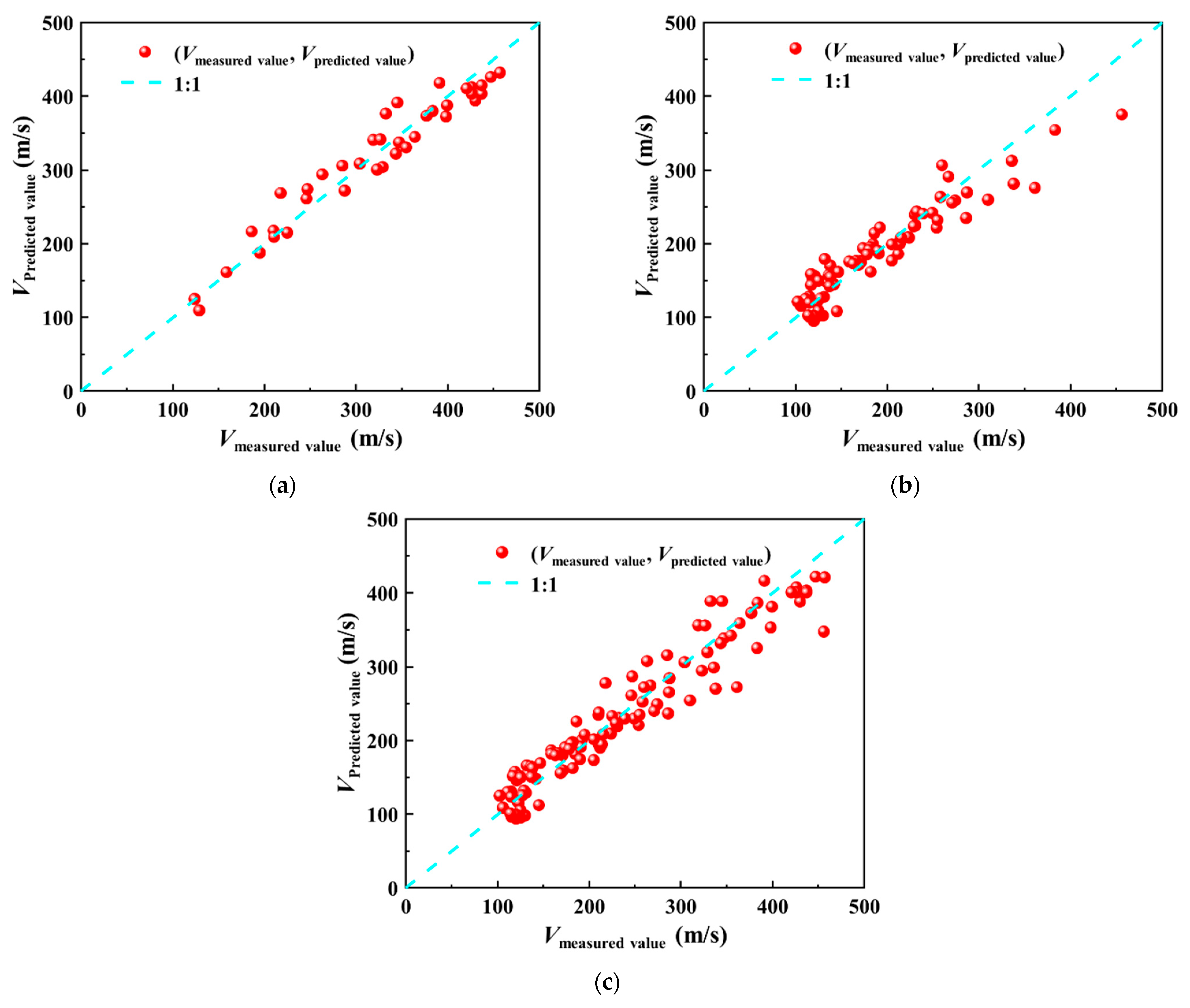
The prediction of shear wave velocity Vs for different soils based on regression equations and the comparative analysis of measured and predicted values were carried out as shown in Figure 2. The predicted and measured values are all near the 1:1 line, demonstrating that the predicted values have a small relative error to the measured values and are strongly correlated for each soil type.

4. Regression Model Evaluation

4.1. Comparative Analysis with Existing Regression Models

Combined with the regression models of shear wave speeds proposed by related scholars for different types of soils, as shown in Table 1, we compare and analyze the reasonableness of the regression models established in this study.

4.1.1. Sandy Soil

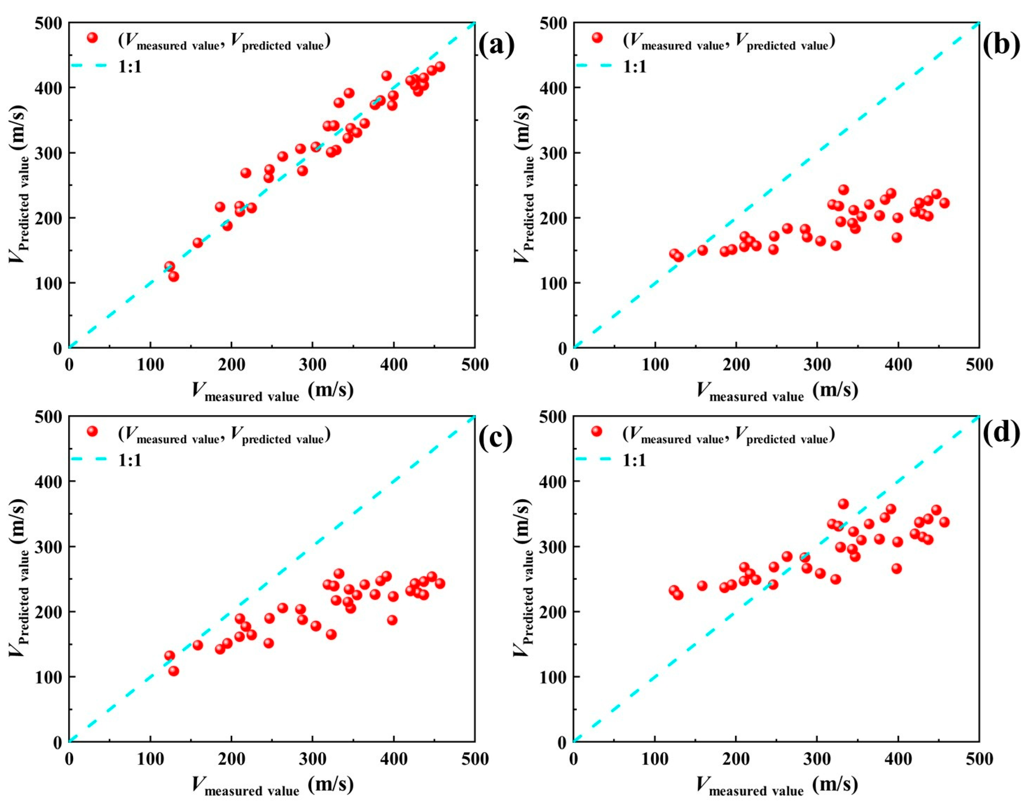
A comparison between measured and predicted shear wave velocity in sandy soil is shown in Figure 3. From Figure 3a, the data points are roughly evenly distributed on both sides of the 1:1 line, which indicates that the new model for sandy soils has a better prediction. In contrast, in Figure 3b,c, the data points both deviate from the 1:1 line as a whole and are concentrated below the line, suggesting that there is a general underestimation of predicted value by the model. From Figure 3d, the mid-range data points closely fit the 1:1 line, indicating that the model predicts moderate shear wave velocity better, but the extremes are not sufficiently reliable. Discreteness at both ends may be due to the model not covering the full range of data features. A possible reason why existing predictive models fail to reasonably estimate shear wave velocity is that the available monitoring datasets do not sufficiently cover a wide range of special sand conditions (e.g., gap-graded soil [35] or soils affected by overconsolidation) and therefore cannot adequately capture the structural state of the soil.

4.1.2. Clay

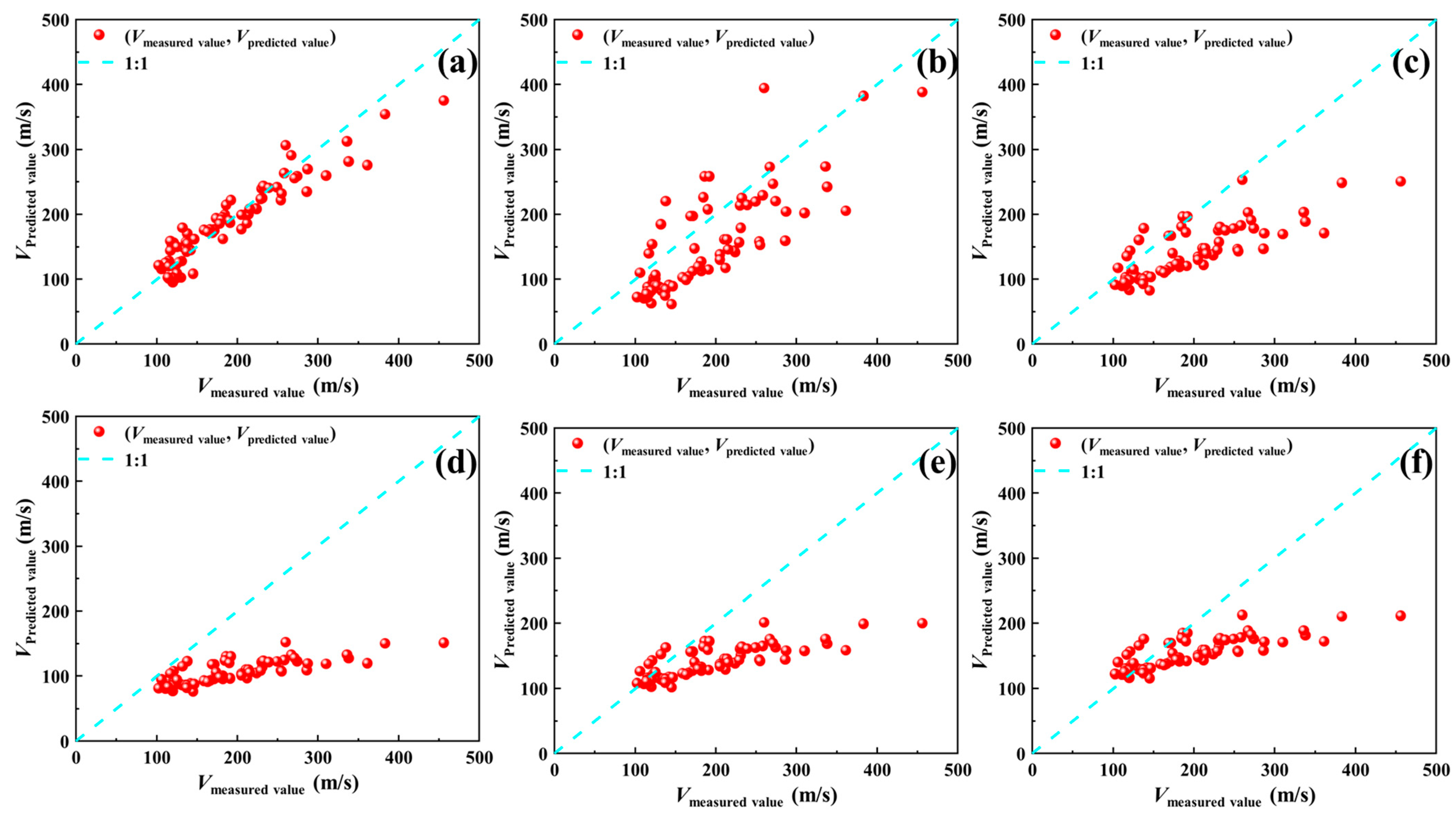
A comparison between measured and predicted shear wave velocity in clay is shown in Figure 4. From Figure 4a, the data points are closely centered around the 1:1 line, which indicates that the prediction accuracy of the new model is high. From Figure 4b, it can be seen that the data points are more symmetrically distributed on both sides of the 1:1 line, but relatively dispersed, and the prediction effect of the model is poor. From Figure 4c–f, it can be seen that the data points are closely centered around the 1:1 line at low shear wave speeds, but as the shear wave speeds increase, the data points begin to deviate from the 1:1 line and are concentrated below the 1:1 line, which suggests that the predictions of these models are reliable when the shear wave speeds are low, but if the speeds are too high, the prediction errors of them also increase. A possible reason is that, for soft-to-medium clays, shear wave velocity is primarily controlled by soil plasticity and water content, which exhibit a strong correlation with cone penetration resistance. In contrast, for stiff and overconsolidated clays, shear stiffness cannot be directly inferred from cone penetration resistance or buried depth.

4.1.3. General Soil

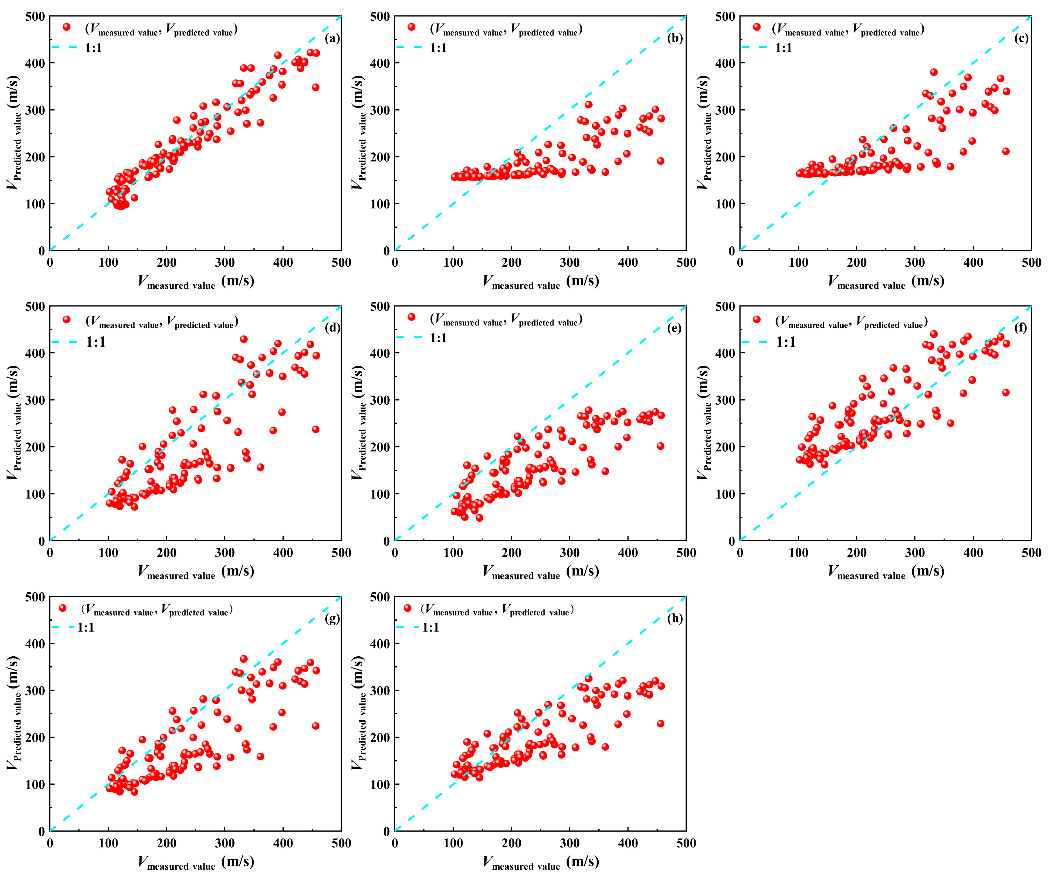
A comparison between measured and predicted shear wave velocity in general soil is shown in Figure 5. As can be seen from Figure 5a, the data points are densely distributed near the 1:1 line, and the overall trend is highly consistent with the 1:1 line, especially in the low shear wave speed to medium speed interval, which indicates that the new model proposed in this paper has high prediction accuracy and fitting effect. From Figure 5b,c, the distribution of data points in the low shear wave velocity section is fair, but most of the points in the high shear wave velocity section are located below the 1:1 line. The model is still reliable under low shear wave velocity conditions, but the prediction error increases as the velocity increases. From Figure 5d, the distribution of data points is slightly dispersed, and although a part of the whole is close to the 1:1 line, there is still a significant deviation in the region of medium and high shear wave velocity, and there is still a systematic underestimation of the medium and high shear wave velocity in this model. From Figure 5e,h, the data points are deviated from the 1:1 line and are scattered, with most of the points below the 1:1 line, and there is a general underestimation. From Figure 5f, it can be seen that the low shear wave velocity performs well, and the data points are close to the 1:1 line, but as the speed increases, the points begin to be upwardly biased, the error expands, and the model has limitations. From Figure 5g, most of the points deviate from the 1:1 line, especially the middle and high shear wave velocity, which are obviously downwardly biased; in addition, the distribution is more dispersed, and the predicted values of the model are generally low, the overall accuracy of the model is poor, and the reliability is not high.
In summary, it can be seen that for sandy soils, clay, and general soils, the distribution of data points predicted by the new regression model is more centralized, with all being distributed near the 1:1 line, and the distribution of data points is more uniform. The shear wave velocity predicted by the new regression model has fewer errors than the measured value. The new model proposed in this paper has the highest prediction accuracy, and the fitting effect is the best.

4.2. Graphical Analysis

4.2.1. Evaluation Metric Establishment

The reliability of the newly proposed regression mode was assessed by four indexes: root mean square error (RMSE) [36,37], the statistics of the mean and standard deviation of the ratio of the fitted shear wave velocity to the measured shear wave velocity (K) [38], ranking index (RI) [39], and ranking distance (RD) [40].
RMSE quantifies the magnitude of the model prediction error. Smaller RMSE values indicate more accurate fitting results. This is determined by using the following equation:
R M S E = 1 N i = 1 N ( y i y ^ i ) 2
The statistics of the mean and standard deviation of the ratio of the fitted shear wave velocity to the measured shear wave velocity (K) are determined by
K = V s c / V s m
RI is able to test the relative accuracy of the regression model, which is determined by
R I = μ l n ( K ) + σ l n ( K )
The magnitude of ranking distance (RD) can effectively reveal the stability of the model. This is determined by
R D = ( 1 μ ( K ) ) 2 + ( σ ( K ) ) 2
where y i is the measured value, y ^ i is the predicted value, N is the number of samples, V s m is the measured value, V s c is the predicted value, and μ and σ represent the mean and standard deviation of the analyzed data series, respectively. The smaller the RMSE, K, RI, and RD are, the better the fit is. Evaluation index calculation results are shown in Table 2.

4.2.2. Evaluation Methods Based on Cumulative Frequency Curves

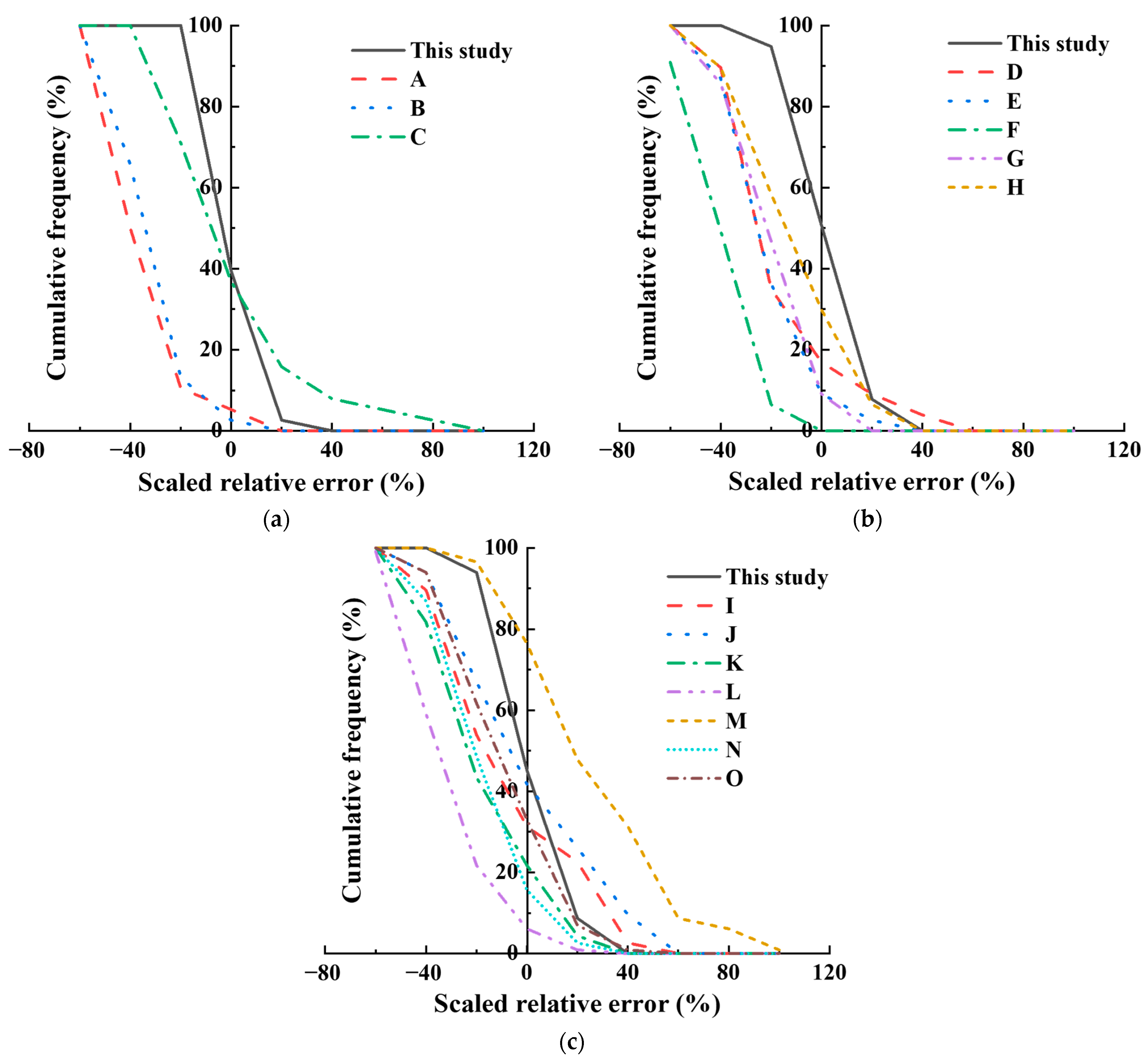
A probabilistic statistical approach was employed to quantitatively analyze the relative error [41]. Cumulative frequency curves were used to assess the error value of the prediction results of the regression model. Scaled relative errors of predicted Vs values are shown in Figure 6. The horizontal axis represents the relative error between the predicted and measured shear wave velocity values, while the vertical axis denotes the percentage of points with errors less than or equal to a given value, i.e., the cumulative frequency. For sandy soils, the cumulative frequency of the newly proposed regression model is approximately 40% at a relative error of 0 in the prediction results, with the greatest prediction accuracy and a relatively small error interval. For clay, the probability of accurate prediction of the newly proposed regression model is about 50%, which has the highest prediction accuracy among all the regression models, and the error interval is relatively small. For general soil, the accurate prediction probability of the newly proposed regression model is about 45%, which is smaller than that of the regression model M. However, the error interval of the model M is too large; that is, the prediction results are discrete. Overall, the regression model proposed in this study has a high prediction accuracy with low errors.

4.3. The Statistical Assessment Method

The regression model is evaluated based on a new statistical assessment method considering the position of the points. A perfect prediction would be Vmeasured value = Vpredicted value, as shown by the 1:1 line in Figure 2. The distance from the point to the 1:1 line can be given by
D i = 2 2 · | V m e a s u r e d   v a l u e V p r e d i c t e d   v a l u e |
In order to show the trend in the curve, a specific straight line from point D90 to point D10 was used. Distance from the perfect line is shown in Figure 7.
K i = | D 90 i D 10 i | | 90 10 |
The perfect distance allows a clearer description of the relative positional relationships from a graphical point of view and corrects the evaluation results. The results show that for sandy soils, clay, and general soil, the K value of the regression model proposed in this study is the maximum, which means that the prediction results of the regression model proposed in this paper have the smallest distance from the 1:1 line and the best prediction results.
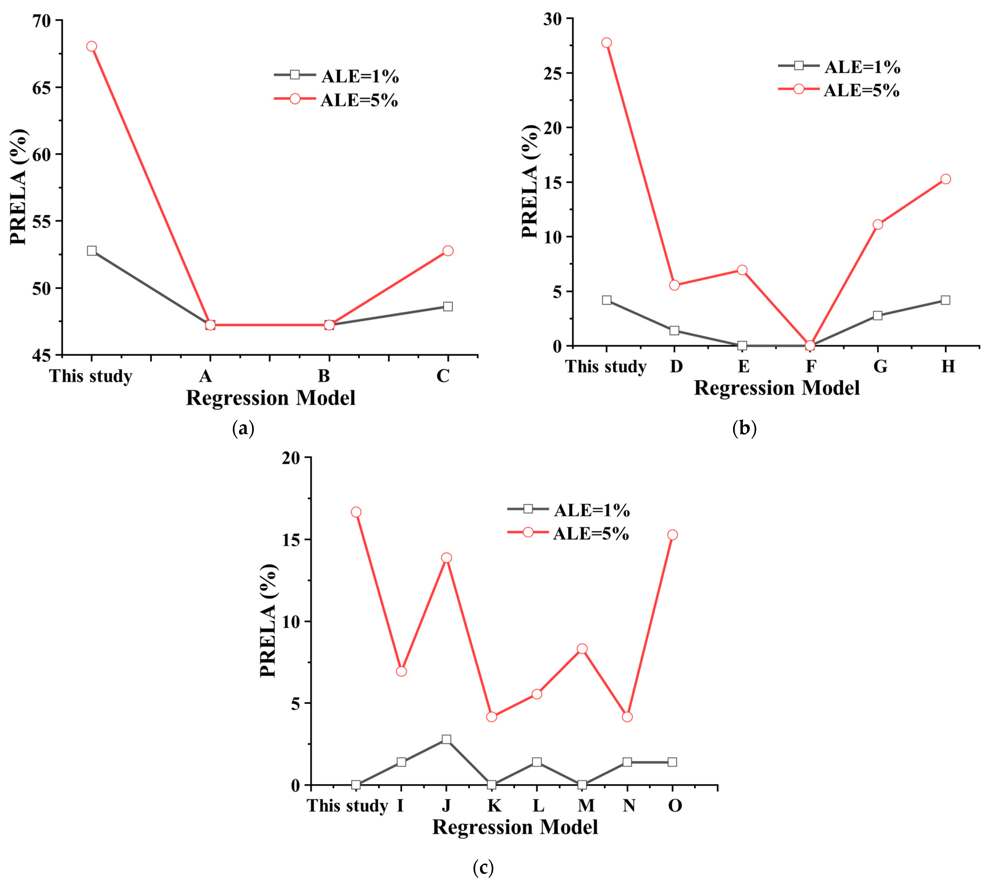
In this study, the relative errors of 5% and 1% between predicted and measured values were counted. The percentage of relative error less than the ALE (PRELA) is shown graphically in Figure 8. The higher the PRELA, the better the correlation performance. For both sandy soils and clay, the PRELA values of the newly proposed regression model are the largest, including 68.06% for sandy soils and 27.78% for clay when ALE = 5%. This indicates that the correlation between the newly proposed model and the measured values is better and the prediction results are more accurate. For general soils, the PRELA value at ALE = 5% is the largest, with a value of 16.67%, but the value is minimized at ALE = 1%. The prediction of the newly proposed model is the best within 5% of the error allowance.

5. Conclusions

The correlation between shear wave velocity Vs, cone penetration resistance Ps, and burial depth H was investigated based on the soft soil layers in Shanghai. A new shear wave velocity regression model was constructed, and the regression model was evaluated. The proposed model is able to capture the complex interrelationships in soil behavior more effectively than traditional single-parameter correlations, thereby significantly reducing prediction uncertainty. The main conclusions obtained are as follows:
(1)
Existing regression models of shear wave velocity Vs and cone penetration resistance Ps were collected and analyzed, and the regression models of shear wave velocity Vs and cone penetration resistance Ps with burial depth H were established. It is found that the existing regression model of shear wave velocity Vs and cone penetration resistance Ps is not applicable to the prediction of shear wave velocity in soft soil layers.
(2)
The regression models of shear wave velocity Vs and cone penetration resistance Ps versus burial depth H for three types of soils are developed, and the evaluation of the new models is assessed by existing regression models, graphical analysis, and statistical assessment methods. At ALE = 5%, the PRELA of sandy, clay, and general soils are 68.06%, 27.78%, and 16.67%, respectively. The predicted shear wave velocity Vs of the newly proposed model in sandy, clay, and general soils agrees best with the monitoring values.
(3)
The new model has higher applicability and accuracy in Shanghai, which can provide a more reliable theoretical basis for engineering geological evaluation and seismic design.
In the future, the newly proposed correlation model relating shear wave velocity to cone penetration resistance holds significant research potential. This model offers a cost-effective and efficient approach for shear wave velocity prediction in soft soil layers and provides a valuable reference for studies under similar geological conditions, when the soft soil deposits share a similar geological origin to those of Shanghai. As monitoring datasets expand and analytical methods advance, future studies should focus on in-depth data mining, optimization, and innovation of model algorithms, aiming to quantify the uncertainty of input parameters (such as qc and H) in prediction and thereby improve model structure and interpretability.

Author Contributions

Conceptualization, H.C. and Z.H.; methodology, Z.H.; formal analysis, H.C.; investigation, Q.H. and Q.W.; data curation, Q.H. and Q.W.; writing—original draft preparation, H.C.; writing—review and editing, H.C. and Z.H.; supervision, Z.H.; funding acquisition, Z.H. All authors have read and agreed to the published version of the manuscript.

Funding

This research was funded by National Natural Science Foundation of China (Grants No. 52478410, 52408436, and 52408435), Shanghai Science and Technology Committee Program (Grants No. 23DZ1202806 and 22dz1201202), The Science and Technology Plan Project of Qinghai Province (No.2023-QY-206), the Open Fund Support Project of Research and Development Center of Transport Industry of New Generation of Artificial Intelligence Technology under Grant No. 202501H, and the Fundamental Research Funds for the Central Universities.

Institutional Review Board Statement

Not applicable.

Informed Consent Statement

Not applicable.

Data Availability Statement

The original contributions presented in the study are included in the article. Further inquiries can be directed to the corresponding author.

Conflicts of Interest

The authors declare no conflicts of interest.

References

  1. Ohta, Y.; Goto, N. Empirical shear wave velocity equations in terms of characteristic soil indexes. Earthq. Eng. Struct. Dyn. 1978, 6, 167–187. [Google Scholar] [CrossRef]
  2. Li, Z.-H.; Xie, J.-J.; Li, K.-W.; Wen, Z.-P.; Li, X.-J.; Wang, Z.-C.; Xu, H.-T.; Zhao, X.-F.; Zhang, N. Empirical extrapolation model of site shear wave velocity and its applicability in Shandong Province. Seismol. Geol. 2024, 46, 934–954. (In Chinese) [Google Scholar]
  3. Olutoki, J.O.; Zhao, J.G.; Siddiqui, N.A.; Elsaadany, M.; Haque, A.E.; Akinyemi, O.D.; Said, A.H.; Zhao, Z. Shear wave velocity prediction: A review of recent progress and future opportunities. Energy Geosci. 2024, 5, 100338. [Google Scholar] [CrossRef]
  4. Bekdaş, G.; Aydın, Y.; Işıkdağ, U.; Nigdeli, S.M.; Hajebi, D.; Kim, T.-H.; Geem, Z.W. Shear Wave Velocity Prediction with Hyperparameter Optimization. Information 2025, 16, 60. [Google Scholar] [CrossRef]
  5. Wang, J.-Y.; Tao, X.-S.; Wang, C.; Shao, B.; Xu, Y. Correlation analysis between shear wave velocity and soil layer depth in urban area of Yancheng City. J. Disaster Prev. Mitig. Eng. 2024, 44, 1193–1201. (In Chinese) [Google Scholar]
  6. Zheng, M.; Huang, Y.-M.; Liang, J.-W.; He, S.-Y.; Li, X.-D.; Chen, H.-W.; Su, B.; Su, X.-M.; Xie, C. Correlation analysis of shear wave velocity and burial depth in rock and soil in the Yulin Area. Earthquake 2024, 44, 78–93. (In Chinese) [Google Scholar]
  7. Lu, D.W.; Sun, Y.H.; Liu, H.S. Reliability evaluation of empirical formula between shear wave velocity and depth of conventional soils. J. Jilin Univ. (Earth Sci. Ed.) 2024, 54, 546–557. (In Chinese) [Google Scholar]
  8. Xu, Y.; Wu, Q.; Fang, Y.; Chen, G.-X. Evaluation method of shear wave velocity of various marine soils in the Lingdingyang Bay. J. Disaster Prev. Mitig. Eng. 2023, 43, 956–964. (In Chinese) [Google Scholar]
  9. Parvizi, S.; Kharrat, R.; Asef, M.R.; Jahangiry, B.; Hashemi, A. Prediction of the shear wave velocity from compressional wave velocity for Gachsaran Formation. Acta Geophys. 2015, 63, 1231–1243. [Google Scholar] [CrossRef]
  10. Oloruntobi, O.; Butt, S. The shear-wave velocity prediction for sedimentary rocks. J. Nat. Gas Sci. Eng. 2020, 76, 103084. [Google Scholar] [CrossRef]
  11. Omovie, S.J.; Castagna, J.P. Estimation of shear-wave velocities in unconventional shale reservoirs. Geophys. Prospect. 2021, 69, 1316–1335. [Google Scholar] [CrossRef]
  12. Kim, J.; Kim, B.; Cho, H. Shear wave velocity estimation in Korea using P-wave seismograms. KSCE J. Civ. Eng. 2020, 24, 3650–3658. [Google Scholar] [CrossRef]
  13. Ismail, A.; Azadbakht, S.; Rashid, H.M.A.; Yasin, Q.; Liu, B.; Ijaz, W. Statistical and machine learning hybridization for predicting shear wave velocity in tight sand reservoirs: A case study. Geoenergy Sci. Eng. 2023, 231, 212420. [Google Scholar] [CrossRef]
  14. Nasrnia, B.; Falahat, R. Studying the Accuracy and Generalizability of Different Estimation Methods of Shear Wave Velocity. Arab. J. Sci. Eng. 2024, 50, 14961–14975. [Google Scholar] [CrossRef]
  15. Liu, Y.; Gao, C.; Zhao, B. Shear-wave velocity prediction based on the CNN-BiGRU integrated network with spatiotemporal attention mechanism. Processes 2024, 12, 1367. [Google Scholar] [CrossRef]
  16. Hazbeh, O.; Rajabi, M.; Tabasi, S.; Lajmorak, S.; Ghorbani, H.; Radwan, A.E.; Alvar, M.A.; Molaei, O. Determination and investigation of shear wave velocity based on one deep/machine learning technique. Alex. Eng. J. 2024, 92, 358–369. [Google Scholar] [CrossRef]
  17. Feng, G.; Zeng, H.-H.; Xu, X.-R.; Tang, G.-Y.; Wang, Y.-X. Shear wave velocity prediction based on deep neural network and theoretical rock physics modeling. Front. Earth Sci. 2023, 10, 1025635. [Google Scholar] [CrossRef]
  18. Cai, R.; Peng, T.; Luo, D.-L.; Zhou, Y.-D.; Yin, X.-X.; Guo, P.; Peng, J.-C. Correlation between the shear wave velocity and the soil depth in Chengdu Region. J. Seismol. Res. 2022, 45, 498–508. (In Chinese) [Google Scholar]
  19. Zhang, X.; Zhang, H.; Yun, M.; Wang, F. Research on shear-wave velocity profile VS30 estimation model in Xiong’an New District. Technol. Earthq. Disaster Prev. 2022, 17, 401–408. (In Chinese) [Google Scholar]
  20. Zekkos, D.; Sahadewa, A.; Woods, R.D.; Stokoe, K.H. Development of model for shear-wave velocity of municipal solid waste. J. Geotech. Geoenviron. Eng. 2014, 140, 04013030. [Google Scholar] [CrossRef]
  21. Damm, J.C.; Lewis, M.R.; Stokoe, K.H.; Moore, D.P. Comparison of in situ and laboratory shear wave velocity measurements in compacted backfill. Geotech. Test. J. 2013, 36, 515–523. [Google Scholar] [CrossRef]
  22. Tsiambaos, G.; Sabatakakis, N. Empirical estimation of shear wave velocity from in situ tests on soil formations in Greece. Bull. Eng. Geol. Environ. 2011, 70, 291–297. [Google Scholar] [CrossRef]
  23. Mayne, P.W.; Rix, G.J. Correlations between shear wave velocity and cone tip resistance in natural Clays. Soils Found. 1995, 35, 107–110. [Google Scholar] [CrossRef]
  24. Dikmen, U. Statistical correlations of shear wave velocity and penetration resistance for soils. J. Geophys. Eng. 2009, 6, 61–72. [Google Scholar] [CrossRef]
  25. Robertson, P.K.; Campanella, R.G. Interpretation of cone penetration tests. Part I: Sand. Can. Geotech. J. 1983, 20, 718–733. [Google Scholar] [CrossRef]
  26. Fear, C.E.; Robertson, P.K. Estimating the undrained strength of sand: A theoretical framework. Can. Geotech. J. 1995, 32, 859–870. [Google Scholar] [CrossRef]
  27. Karray, M.; Lefebvre, G.; Ethier, Y.; Bigras, A. Influence of particle size on the correlation between shear wave velocity and cone tip resistance. Can. Geotech. J. 2011, 48, 599–615. [Google Scholar] [CrossRef]
  28. Brignoli, E.M.; Gotti, M.; Stokoe, K.H. Measurement of shear waves in laboratory specimens by means of piezoelectric transducers. Geotech. Test. J. 1996, 19, 384–397. [Google Scholar] [CrossRef]
  29. Ansal, A.; Iyisan, R.; Güllü, H. Microtremor Measurements for the Microzonation of Dinar. Pure Appl. Geophys. 2001, 158, 2525–2541. [Google Scholar] [CrossRef]
  30. Ansal, A.; Iyisan, R.; Yldrm, H. The cyclic behaviour of soils and effects of geotechnical factors in microzonation. Soil Dyn. Earthq. Eng. 2001, 21, 445–452. [Google Scholar] [CrossRef]
  31. Tun, M.; Ayday, C. Investigation of correlations between shear wave velocities and CPT data: A case study at Eskisehir in Turkey. Bull. Eng. Geol. Environ. 2018, 77, 225–236. [Google Scholar] [CrossRef]
  32. Madiai, C.; Simoni, G. Shear wave velocity-penetration resistance correlation for Holocene and Pleistocene soils of an area in central Italy. In Geotechnical and Geophysical Site Characterization, Proceedings of the Second International Conference on Site Characterization, ISC-2, Porto, Portugal, 19–22 September 2004; IOS Press: Amsterdam, The Netherlands, 2004; Available online: https://www.researchgate.net/publication/237326403 (accessed on 22 July 2025).
  33. Hegazy, Y.A.; Mayne, P.W. A global statistical correlation between shear wave velocity and cone penetration data. In Site and Geomaterial Characterization; ASCE: Reston, VA, USA, 2006; pp. 243–248. [Google Scholar] [CrossRef]
  34. Tong, L.Y.; Che, H.B.; Zhang, M.F.; Li, H.J. Review of shear-wave velocity prediction equations based on piezocone penetration test data: Example from Yangtze River floodplain deposits at Nanjing, Jiangsu Province, China. Q. J. Eng. Geol. Hydrogeol. 2018, 51, 229–246. [Google Scholar] [CrossRef]
  35. Zhang, D.-M.; Chen, H.-H.; Xie, X.-C.; Chen, S.-R.; Chen, Z.-G.; Li, J.-P. Multiscale responses of gap-graded soil under the combined effect of train vibration and seepage erosion. Transp. Geotech. 2025, 55, 101669. [Google Scholar] [CrossRef]
  36. Liu, Z.; Fan, S.; Liu, S.-L.; Zhao, A.-R.; Liu, L. Research on prediction of pigment concentration in color painting based on BOA-FRNN spectral model. Spectrosc. Spect. Anal. 2025, 45, 322–331. (In Chinese) [Google Scholar]
  37. Grima, A.; Babuška, R. Fuzzy model for the prediction of unconfined compressive strength of rock samples. Int. J. Rock Mech. Min. Sci. 1999, 36, 339–349. [Google Scholar] [CrossRef]
  38. Briaud, J.-L.; Tucker, L.-M. Measured and predicted axial response of 98 piles. J. Geotech. Eng. 1988, 114, 984–1001. [Google Scholar] [CrossRef]
  39. Hu, Q.-Z.; Lu, H.-P.; Yang, Y.-N.; Cheng, N. Dynamic comprehensive measure model based on information degree and order exponent. Syst. Eng. Electron. 2011, 33, 816–820. (In Chinese) [Google Scholar]
  40. Orr, T.L.; Cherubini, C. Use of the ranking distance as an index for assessing the accuracy and precision of equations for the bearing capacity of piles and at-rest earth pressure coefficient. Can. Geotech. J. 2003, 40, 1200–1207. [Google Scholar] [CrossRef]
  41. Huang, Z.-K.; Zeng, N.-C.; Zhang, D.-M.; Argyroudis, S.; Mitoulis, S.-A. Resilience Models for Tunnels Recovery After Earthquakes. Engineering 2025, 6, 28. [Google Scholar] [CrossRef]
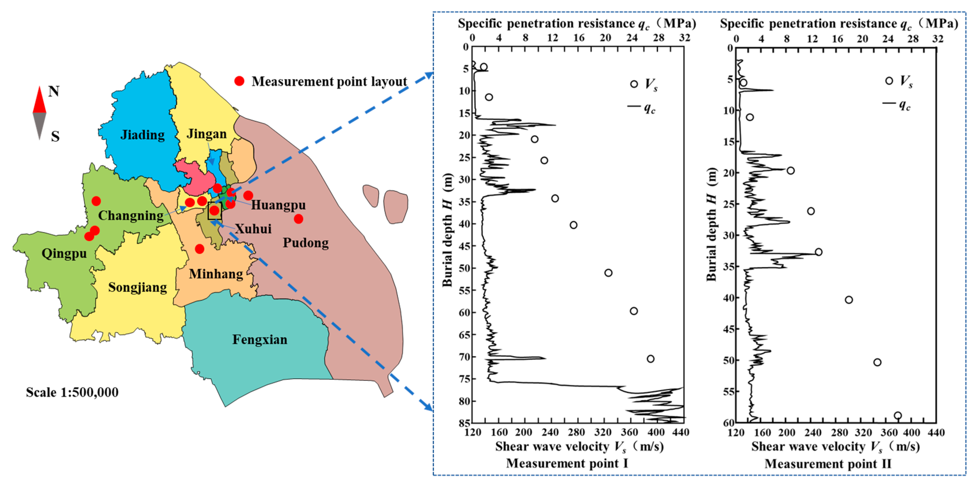
Figure 1. Borehole location map.
Applsci 15 10065 g001
Figure 2. Comparison between measured and predicted shear wave velocity: (a) sandy soil; (b) clay; (c) general soil.
Applsci 15 10065 g002
Figure 3. Comparison between measured and predicted shear wave velocity: (a) The newly proposed model; (b) Model A; (c) Model B; (d) Model C.
Applsci 15 10065 g003
Figure 4. Comparison between measured and predicted shear wave velocity: (a) The newly proposed model; (b) Model D; (c) Model E; (d) Model F; (e) Model G; (f) Model H.
Applsci 15 10065 g004
Figure 5. Comparison between measured and predicted shear wave velocity: (a) The newly proposed model; (b) Model I; (c) Model J; (d) Model K; (e) Model L; (f) Model M; (g) Model N; (h) Model O.
Applsci 15 10065 g005
Figure 6. Scaled relative errors of predicted Vs values: (a) sandy soil; (b) clay; (c) general soil.
Applsci 15 10065 g006
Figure 7. Distance from the perfect line: (a) sandy soil; (b) clay; (c) general soil.
Applsci 15 10065 g007
Figure 8. Results of the PRELA: (a) sandy soil; (b) clay; (c) general soil.
Applsci 15 10065 g008
Table 1. The regression model between cone penetration resistance qc and shear wave velocity Vs.
Soil TypeNo.Regression Model FormReferences
Sandy soilA V s = 134 + 0.52 q c Stokoe (1983) [20]
B V s = 54.8 ( q c ) 0.29 Stokoe (1983) [21]
C V s = 218 + 0.70 q c Iyisan (1996) [22]
ClayD V s = 1.75 ( q c ) 0.627 Mayne and Rix (1995) [23]
E V s = 55.3 ( q c ) 0.377 Iyisan (1996) [24]
F V s = 102 ( q c ) 0.23 Robertson et al. (1992) [25]
G V s = 135 ( q c ) 0.23 Fear and Robertson (1995) [26]
H V s = 149 ( q c ) 0.205 Karray (2011) [27]
General soilI V s = 154 + 0.64 q c Barrow and Stokoe (1983) [28]
J V s = 160 + 0.9 q c Iyisan and Ansal (1993) [29]
K V s = 45 ( q c ) 0.41 Iyisan and Ansal (1993) [30]
L V s = 109.29 + 52.674 L n ( q c ) Tun (2003) [31]
M V s = 211 ( q c ) 0.23 Madiai and Simoni (2004) [32]
N V s = 11.711 ( q c ) 0.3409 Hegazy and Mayne (2001) [33]
O V s = 28.45 ( q c ) 0.241 Tong (2017) [34]
Note: The CPT cone penetration resistance qc unit is in kPa, and the shear wave velocity Vs unit is in meters (m/s).
Table 2. Evaluation index calculation results.
Soil TypeNo.RMSEKRIRD
%<1MeanSD
Sandy soilX23.14752.7781.0030.0820.0790.082
A146.37747.2220.6390.1630.7050.396
B129.88047.2220.6750.1300.5950.350
C68.86048.6110.9930.2720.2800.272
ClayY25.6214.1671.0090.1370.1350.137
D60.6091.3890.7970.2460.5400.319
E69.17600.7690.1690.4930.286
F103.62400.5970.1400.7850.427
J75.5912.7780.7900.1850.5040.280
H67.3624.1670.8730.2100.4160.246
General soilZ28.45101.0070.1320.1320.132
I84.0461.3890.9070.2760.4480.291
J68.3132.7880.9830.2750.3410.276
K70.83400.7990.2190.5290.297
L95.6991.3890.6730.1730.6670.370
M62.25201.2430.2900.4230.378
N72.4941.3890.7970.1840.4820.274
O68.5421.3890.8930.2050.3680.231
Disclaimer/Publisher’s Note: The statements, opinions and data contained in all publications are solely those of the individual author(s) and contributor(s) and not of MDPI and/or the editor(s). MDPI and/or the editor(s) disclaim responsibility for any injury to people or property resulting from any ideas, methods, instructions or products referred to in the content.