Article

Data-Driven Tracing and Directional Control Strategy for a Simulated Continuum Robot Within Anguilliform Locomotion

Group of Biomechatronics, Fachgebiet Biomechatronik, Technische Universität Ilmenau, D-98693 Ilmenau, Germany
*
Author to whom correspondence should be addressed.
Appl. Sci. 2025, 15(18), 10045; https://doi.org/10.3390/app151810045 (registering DOI)
Submission received: 20 July 2025 / Revised: 2 September 2025 / Accepted: 12 September 2025 / Published: 14 September 2025
(This article belongs to the Special Issue Application of Computer Science in Mobile Robots II)

Abstract

Biorobotics leverages the principles of natural locomotion to enhance the mobility of bioinspired aquatic robots. Among various swimming modes, anguilliform locomotion is particularly recognized as an energy-efficient mode incorporating complex multiphysics. Due to whole-body undulation, the determination of the anguilliform swimmer’s direction is not trivial. Furthermore, the neuromuscular mechanism that controls straight swimming is not fully understood. This study investigates the challenge of predicting and controling the gross motion trajectory of a soft robot that utilizes anguilliform swimming. The robot consists of a six-segment continuous body, where each segment is actuated with pneumatic artificial muscles. A mode extraction technique based on dynamic mode decomposition (DMD) is proposed to identify the robot’s future state. Using the complex-variable delay embedding (CDE) technique, the CDE DMD algorithm is developed to predict the robot trajectory trend. To vary the robot direction, a hypothesis that asymmetric sidewise actuation results in slightly different fluid velocities between the left and right sides of the robot was investigated using COMSOL Multiphysics® 6.2. The simulation results demonstrate the CDE DMD’s ability to predict gross motion across various scenarios. Furthermore, integrating the prediction model with the asymmetric actuation rule provides a control strategy for directional stability of the robot. Simulations of the closed-loop system with non-zero initial pose (step response) indicate the performance in maintaining straight-line swimming with approximately a 60s settling time.

1. Introduction

Conventional machines typically use rotary motors as the primary propulsion systems to drive wheels or rotary fans, such as those found in ships. In contrast, nature provides a variety of locomotion mechanisms that are considerably more efficient, particularly in complex and unstructured environments. In aquatic locomotion, to generate propulsion in liquid domains, fishes exhibit various modes such as anguilliform, subcarangiform, carangiform, and thunniform [1]. The Lindsey classification of the fish swimming styles counts twelve modes based on the geometry of the moving region of the fish, and body undulation or oscillation [2,3]. Admittedly, drawing a definite border between the modes is not easy because the modes appear to be kinematically analogous. Nevertheless, the anguilliform mode is particularly distinguishable from the other modes because the whole body is engaged in the undulatory motion, containing the rearward-traveling wave, which provides propulsion for the swimmer. In this mode of locomotion, fins do not play a significant role; therefore, snake-like anatomies, ranging from nematodes to eels, employ an anguilliform mode for locomotion. This can be used for developing robotic systems intended to navigate fluidic environments in different Reynolds numbers (Re).
Designing soft robots to mimic the anatomy and kinematics of aquatic creatures is still state-of-the-art research [4,5,6]. Due to structural compliance, soft robots reflect some phenomena and complexities of natural creatures. On one hand, due to whole-body undulation, there is no physically rigid moving point indicating the motion direction. In anguilliform locomotion, the measurements of any positioning sensor [7] will be contaminated with the body undulation. On the other hand, there is no specified primary actuator, like fins, for creating the necessary yaw torques for straight swimming. In fin-based steering, in fish such as sunfish or perch, dorsal, anal, and caudal fins counteract unwanted body rotations to maintain forward motion.
Due to the lack of pronounced appendages and body flexibility, the directional stability of the slender and elongated fishes, such as eels, lampreys, and larval fishes, relies on kinematics and hydrodynamics. To swim straight, such species may depend on highly symmetric body undulations to produce net forward thrust without lateral deviation [8]. Turning can be seen as a separate problem within the study of anguilliform locomotion. Recent research has shown that snakes twist their bodies inward and shift their center of mass to reduce their moment of inertia during turning behaviors [9]. In [10], it is reported that an eel performs forward motion or distinctive curling behavior depending on some external electrical stimulation. Nevertheless, they concluded that complete control over the eel’s motion (such as the path-following problem) is far more complicated. Within fish, swimming locomotion is classified into two generic categories: steady (employed by the fish over relatively long distances at a constant speed) and transient movements [1]. Similarly, the problem of the elongated robots’ navigation can be divided into steady path following and unsteady maneuvers (including turning).
Robots are prone to errors in their initial pose, disturbance within locomotion, as well as actuator and sensor faults. Therefore, the swimming of a robot along a line needs active control, especially over long distances. Various research is devoted to path planning and trajectory following of elongated robots [11,12,13,14]. Multi-body rigid snake robots can rely on angular deflections added on different joints for turning motion, as formulated in [15]. Researchers employ bionic approaches to improve the motion performance, such as the heading angle for a fish robot [16]. Recently, strategies based on left–right unbalanced amplitude and head steering were experimentally implemented when maneuvering a soft swimming robot [17]. Unlike rotary motors that can rotate to any angle as the reference zero around which the rotor oscillates, soft actuators commonly have a fixed nominal position corresponding to the straight nominal state of the fish robot. Therefore, finding a method for regulating the soft robot’s swimming direction is essential. Researchers employ computational fluid dynamics (CFD) to study the hydrodynamics of anguilliform swimming [18,19]. The classic analytical methods like [20] had limitations in modeling the fluid–body interaction, as well as considering the detailed shape of the swimmer.
Machine learning (ML) techniques are extensively explored to handle various problems, such as gait optimization [19] and analysis of mode shapes resulting from the interaction of the soft body with the surrounding water [21,22] for anguilliform swimming robots. The dynamic mode decomposition (DMD) is a data-driven ML technique that is powerful in uncovering coherent structures within fluid flows and mechanical vibrations [23,24]. The academic world is still witnessing new variants and algorithms for the adoption of diverse problems [25]. Various variants of the DMD algorithm have been developed for forecasting and identification in different scientific applications. The delay embedding technique has demonstrated the capability of decomposing interconnected dynamics, like separating waves and turbulence in fluid dynamics [26,27]. The complex-variable delay-embedded method, CDE DMD, has shown the ability to decompose the underlying modes of anguilliform swimming from experimental data obtained by tracking markers on the midline of a soft eel robot [28]. It was demonstrated that the method isolates the traveling wave dynamics as the result of inherent linear (as understood in the context of DMD) modes.
The directional stability, the term borrowed from fish locomotion, remains an unsolved problem for anguilliform swimming soft robots. The objectives of this study are to develop a method to predict the swimmer’s gross motion and control it. The scope is limited to theoretical algorithm development and simulations. The CDE DMD is explored and modified to provide the prediction model (that can be used like an observer block in a feedback control strategy). The objectives include proposing a control strategy, compatible with pneumatic soft robots (that can be practically feasible within pneumatics). A simulation study was conducted using COMSOL Multiphysics® 6.2 (COMSOL AB, Stockholm, Sweden) to evaluate the directional variation based on unbalanced forcing with nonuniform right–left maximum pressures.
The remaining sections of this article are organized as follows. In Section 2.1, the undulatory motion and the problem of directional stability in anguilliform swimming are explained first. Then, in Section 2.2, the method of CDE DMD and the online prediction formula are derived. Section 2.3 is devoted to explaining the actuation method proposed for generating the control input. The computation and simulation results are presented in Section 3. The prediction formula is first tested in open-loop scenarios, and then in closed-loop control scenarios with initial value errors. In Section 4, the implementation of the results in the actual pneumatic system is discussed. The limitations of closed-loop implementation and suggestions for future work are given in this section. Finally, conclusions are summarized in Section 5.

2. Materials and Methods

2.1. The Problem of Directional Stability

One advantage of anguilliform swimming is its energy efficiency in long-distance movements. Maintaining the swimmer’s direction along the desired direction is the first task raised from the control engineering point of view. The question is how to determine a control strategy to make the swimmer follow a straight line. The issue contains complexities that may be translated into observer and control design in robotics terms. Ideally, inspired by the swimming of salamanders, the simplest kinematics of the traveling waves in anguilliform locomotion can be described by a backward-moving sinusoidal wave, such as
f ( x , t ) = α ( t ) sin ( 2 π x t   v ( t ) γ )
where α ( t ) is the undulation amplitude, γ is the wavelength, and v ( t ) is the wave velocity along the swimming axis x . During steady swimming, both velocity and amplitude remain constant. Nevertheless, achieving such ideal movement is practically very hard due to the imperfect mechanical structure of robots, along with external disturbances. An illustration of the anguilliform swimming kinematics is schematically shown in Figure 1. For comparison, a stable straight motion is shown in Figure 1a. In Figure 1b,c, the swimming involves a uniform tilting to the left and right, respectively. In this case, the undulation time is T, and the tilting involves approximately π / 10 yaw during the period. Although the deviation angle is considerable, its effects appear very slowly in reality because the undulation period for swimming in water contains low frequencies in the range of 100 Hz.
This complexity presents a significant challenge from a control engineering perspective: detecting or identifying directional deviations within a short timeframe during a small portion of the motion cycle, to counteract them using feedback controller gains effectively. Note that the presence of extra modes in practice does make the problem more complicated. A quick detection of a deviation angle, potentially, provides the necessary signal for the steering mechanism to act against the deviation and stabilize the forward motion. Otherwise, if the observer requires several undulations to estimate the tendency, the control process will face a time delay due to measurement time, as well as the fluid dynamics resistance of the water.
The next problem concerning stable swimming is related to the actuation for control purposes. A mechanism is needed that can maintain efficient forward swimming while simultaneously enabling direction adjustments. It is hypothesized that regulating the muscle forces of one side results in a sidewise tendency or yaw motion. However, due to the high density of water, the swimming capability of soft robots is not easily achieved, and the asymmetric actuator force should be minimized. To gain insight into the effects of unbalanced actuation and to identify effective parameters, we propose a particle tracking simulation using COMSOL Multiphysics® 6.2.

2.2. The Proposed CDE DMD Algorithm

The CDE DMD algorithm is a variant of DMD developed to analyze and isolate traveling waves that are highly contaminated with additional noise or stationary modes. The propagation of traveling waves within soft and compliant bodies in the aquatic domain, as in soft robots and real fish, is associated with extra fluctuations. The additional fluctuations are attributed to chaotic hydrodynamic modes as well as external noise. In other words, due to the compliance of the fish (or soft fish robot) body, the midline curvature is subject to the superposition of different mode shapes (not only the pure traveling wave). Besides the challenges of capturing traveling waves within the soft body, the swimming physics is further complicated by the infinite-dimensional nature of the coupled fluid and flexible body dynamics. Capturing the dynamics from a limited set of observables or sensor measurements along the swimmer’s backbone presents an additional layer of complexity. The algorithm augments the position data by adding average velocities obtained by differentiation. The delay embedding handles a data augmentation role by including the past observations. Previous studies have shown that by embedding the past data up to nearly half of the undulation period, the linear modes and pure undulation related to the traveling wave are revealed by the algorithm. The CDE DMD isolates the modes directly from measurement data, enabling analysis, prediction, and control without requiring explicit physical models.
The algorithm is formulated concisely in this section. The method involves tracking data of discrete markers distributed uniformly on the midline of the swimmer’s body. Suppose the state vector at time t = k Δ t is shown by a complex variable, z , k s × 1 , composed of the lateral position and filtered velocity of s digitized points on the robot midline as
z , k = y , k + j v ¯ , k
Note that, in this context, expressions like x , k correspond to a vector or ‘all rows of column k of matrix x’. Similarly, x k , represent a row vector or ‘all column elements of row k’. In this work, the velocities were obtained by differentiation of y , k , and a moving average over the past d steps was used in the calculation of v ¯ , k . Following the technique of delay embedding, the Hankel matrix [29] H s ( d + 1 ) × ( n d ) is constructed by embedding d delayed coordinates as follows:
H = z , 1 + d z , 2 + d z , n z , d z , 1 + d z , n 1 . . . . . . . . . z , 1 z , 2 z , n d
As in the snapshot syntax, the matrix is denoted by its columns h , k representing the kth column of H.
H = | h , 1 | | h , 2 | | h , n d |
Then, a linear operator mapping snapshots of the system dynamics one timestep forward, fundamentally a linear approximation of the Koopman operator, A C s ( d + 1 ) × s ( d + 1 ) , is considered as
h , k + 1 = A h , k
Based on the DMD approach, the best solution can be obtained by solving the matrix equation:
X + = A X
where X + = [ h , 2 , h , 3 , , h , n d ] and X = [ h , 1 , h , 2 , , h , n d 1 ] . The X matrix is decomposed into left singular vectors, U C s ( d + 1 ) × r , a diagonal matrix of singular values, Σ R r × r , and the Hermitian transpose of right singular vectors W C ( n d 1 ) × r using a singular value decomposition (SVD) as
X = U Σ W *
where ‘*’ denotes the Hermitian transpose. Supposing the SVD calculation provides the matrices as
U = | u , 1 | | u , 2 | | u , r | , Σ = σ 1 0 0 σ r , W = | w , 1 | | w , 2 | | w , r |
where σ 1 σ 2 σ r > 0 are chosen the leading singular values. Therefore, a modal decomposition can be expressed as
X = u , 1 σ 1 ( w , 1 ) * + u , 2 σ 2 ( w , 2 ) * + + u , r σ r ( w , r ) *
Generally, in DMD approaches, instead of a full matrix of singular values, a rank-reduced matrix is considered. This results in the elimination of low-energy components, which are commonly associated with noise [24]. This fact makes the algorithm robust to random high-frequency noise. The pseudoinverse matrix, D , satisfying A = X + D , D = W Σ 1 U * is obtained using
D = i = 1 r w , i σ i 1 u i , *
In the CDE DMD analysis of anguilliform locomotion, we are interested in particular modes that compose interesting physical motions, including the pure backward-traveling waves, stationary waves, and, in this research, the rigid or gross motion. Supposing the physics of interest is presented, e.g., by σ k and σ p , the pseudoinverse matrix can be partitioned as
D = D ^ + Re s D
So,
D ^ = w , k σ k 1 u k , * + w , p σ p 1 u p , * , Re s D = i k , p w , i σ i 1 u i , *
Thus, the linear operator, A ^ s ( d + 1 ) × s ( d + 1 ) , corresponding to the specified modes is readily calculated as
A ^ = X + D ^
Note that A ^ relates the current state vector in the embedded coordinates to the following approximate snapshot, shown by z ˜ , corresponding to the relevant modes as in
z ˜ , m + 1 z ˜ , m z ˜ , m d + 1 T = A ^ z , m z , m 1 z , m d T = A ^ h , m d
An eigen decomposition of A ^ is computationally viable, satisfying
A ^ Φ = Φ Λ
Φ = | ϕ , 1 | | ϕ , 2 | | ϕ , n | , Λ = λ 1 0 0 λ n ,
In DMD, the eigenmodes are measured by eigen decomposition of a reduced-order matrix. To exclusively measure the first term, z ˜ , m + 1 , the update rule can be written with the first rows as
z ˜ , m + 1 = i ϕ 1 , i ϕ 2 , i ϕ s , i T λ i ϕ i , h , m d
where ϕ i , are the rows of the pseudo matrix
Φ = ( Φ * Φ ) 1 Φ * = ϕ i ,
When the neutral dynamics, A ^ representing rigid-body motion, possess two eigenvalues equal to one,
ϕ 1 , ϕ 2 , = ( ϕ , 1 ) * ( ϕ , 2 ) * ϕ , 1 ϕ , 2 1 ( ϕ , 1 ) * ( ϕ , 2 ) *
The prediction formula can be simplified as follows:
z ˜ , m + 1 = ϕ 1 , 1 ϕ 2 , 1 ϕ s , 1 T ϕ 1 , h , m d +     ϕ 1 , 2 ϕ 2 , 2 ϕ s , 2 T ϕ 2 , h , m d
The memory allocation for online measurement of h , m d is schematically shown in Figure 2. The current value, h , m d , is updated using the z , m , measured at the time t = m Δ t , and the previous value, h , m d 1 , is shifted in a memory-stacking manner. Then, the updated value is used in (16) to calculate the estimated future value z ˜ , m + 1 . The pseudocode algorithm for online measurement is given in Table 1.

2.3. Actuation Mechanism

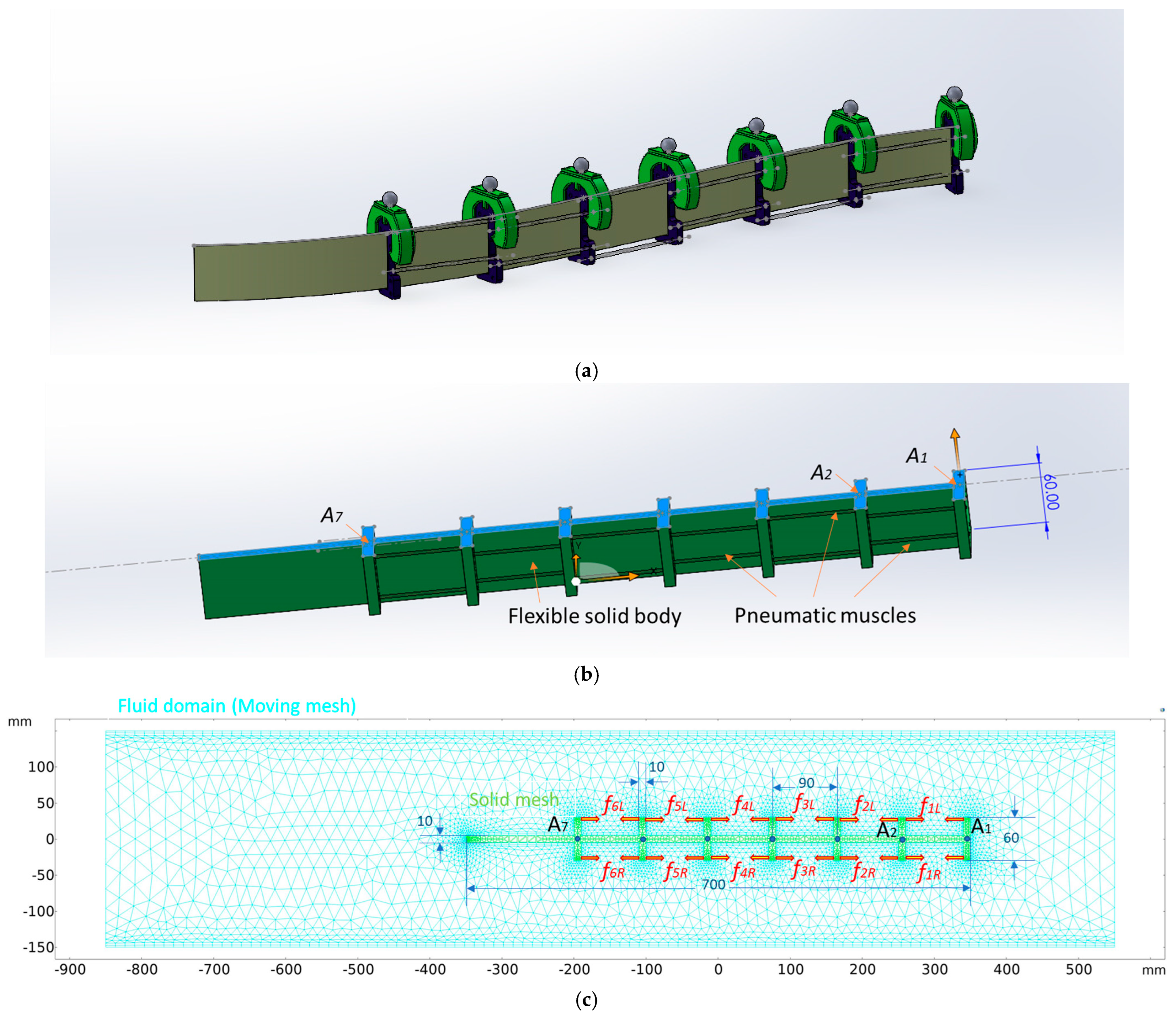
The previous section introduced a state estimator or observer that can be employed for control purposes through embedding in a control rule. In this section, an actuation method for implementing the controller is proposed. The model of the system, as illustrated in Figure 3, shows the robot structure and the actual mesh used within the COMSOL Multiphysics® simulation, similar to the model presented in [21]. The robot body is represented by green elements, with additional annotations providing dimensional and force information. The robot has six segments, and each segment contains lateral contracting-type McKibben actuators that enable the segment to bend to the right or left. The actuator forces are the external forces shown by the red arrows, and their values are related to the actuation sequence.
The finite element (FE) model was developed in a separate study [21] and is reused here. The study models a swimming robot in a shallow water tank using a two-dimensional approach in COMSOL Multiphysics® 6.1, where the fluid is treated as an incompressible laminar flow and the robot’s backbone, floats, and tail are modeled as linear elastic solids with muscle forces applied externally. A fully coupled fluid–structure interaction (FSI) is simulated using the arbitrary Lagrangian–Eulerian (ALE) formulation with a moving mesh method (Yeoh model, stiffening factor C2 = 100) to capture large deformations while maintaining mesh continuity and accuracy near boundaries, corners, and high-gradient regions. Boundary conditions include no-slip walls, an experimentally obtained inflow velocity at the inlet, and fully developed flow at the outlet, with boundary layers and mesh refinement applied for accuracy. The coupled system solves modified Navier–Stokes and solid momentum equations at each time step (0.001 s), with the mesh continuously adapting to the robot’s motion to ensure velocity and stress continuity at the fluid–solid interface, thereby enabling precise simulation of the robot’s locomotion and fluid interactions. In this work, as expressed in Figure 4, the previous model is extended by adding fluid-particle tracing (FPT). The physics-controlled coarse mesh was used for the whole domain. The integrated physics includes laminar flow (SPF), solid mechanics (for the robot body), moving mesh (for fluid domain), FSI, and the FPT. The physical properties of water were assigned to particles with a radius of 0.2 mm to represent water flow, utilizing the Stokes drag law accurately. The simulation is divided into two steps: Study 1 and Study 2, conducted in COMSOL Multiphysics®.
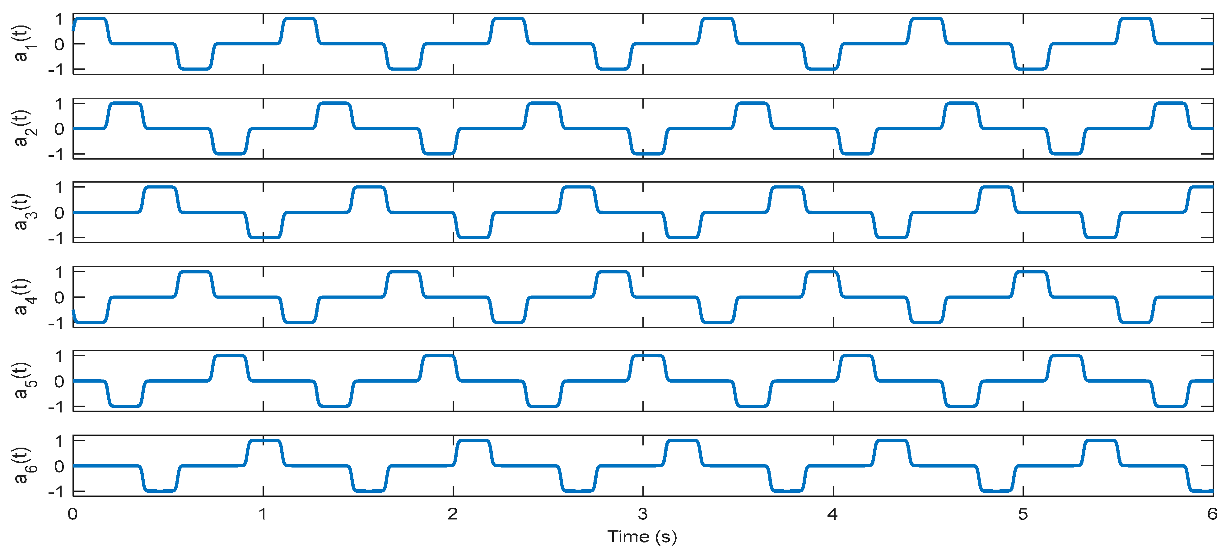
The actuation sequence is represented as a i ( t ) , as shown in Figure 5. The muscle forces are related to pressures P R and P L at the right and left sides (as will be explained later. Thus, for segment numbers i = 1 to 6, the forces can be written as
f i R = a i ( t ) + a i ( t ) 2   P R , f i L = a i ( t ) a i ( t ) 2   P L
In the uncontrolled system, P R = P L = P 1 is supposed to be constant. However, an actuation mechanism or rule is needed to enable the implementation a control strategy. Some hypotheses might be adopted for steering and a change in orientation while swimming. For example, static bending of the dorsal part of the robot should cause a yaw angle. In this study, we needed a solution with minimal change in the actuation so that the control input does not influence swimming performance. Therefore, for an unbalanced actuation, we suppose a slightly reduced pressure, P 2 = 1 δ 0 P 1 , and a direction parameter δ δ 0 , 0 , δ 0 , so that
P R = P 1 1 max ( 0 , δ ) , P L = P 1 1 max ( 0 , δ )
To investigate how a slightly unbalanced forcing may affect material passage within the scope of CFD, a particle-tracing study was performed. Note that the unbalance factor can be related to a heuristic control rule expressed as
δ = sgn ( K z ˜ , m + 1 ) δ 0
where ℜ denotes the real part of the complex variable, sgn refers to the sign function, and K is the control gain for the simple case of a linear proportional controller.

3. Results

3.1. Particle Tracing

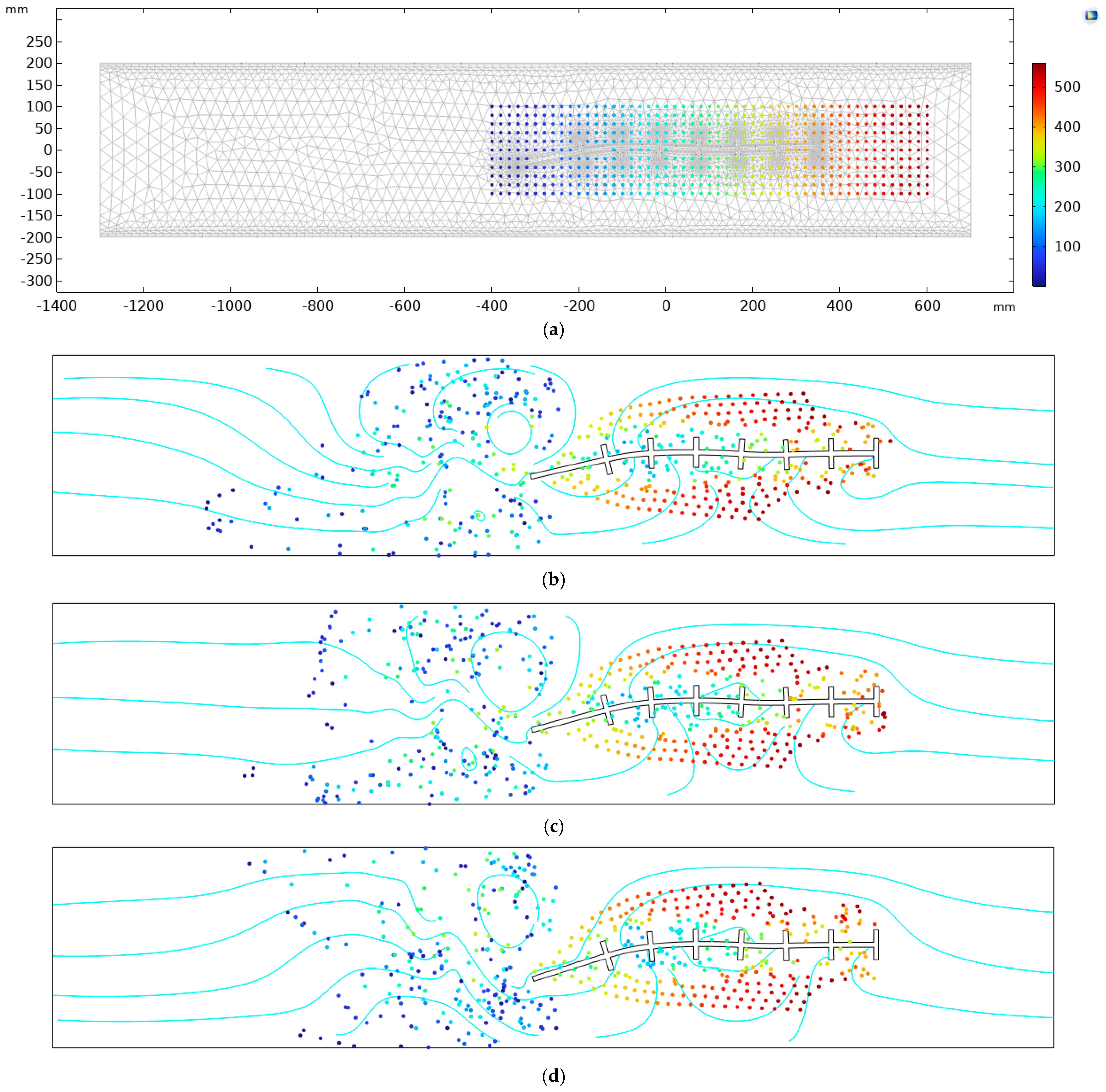
Results of CFD (FSI analysis, in better words) are presented in visualized graphs, like velocity and pressure fields. However, visualization of material (particle) movement is much more comprehensible than the vector fields to describe the robot relative motion. Unlike Eulerian methods, which observe flow at fixed spatial points, FPT follows individual particles, providing direct insight into the material transport. The FPT simulation results for three (open-loop) scenarios are shown in Figure 6. The FPT result for asymmetric actuation, where the left muscles exert a slightly stronger force than the right side, is presented in Figure 6b.
In Figure 6c, the corresponding result for balanced forcing is shown. For comparison, the simulation result accentuating the right-side forces is given in Figure 6d. The comparison shows that an asymmetric actuation causes asymmetric material movement of the flow concerning the robot head. In other words, the relative motion of the swimmer on the accentuated side is more than on the other side.
First, in Study 1, the time-dependent analysis is performed without computing the particle tracing. In Study 2, only the FPT is solved. In this step, the results of the time-dependent analysis from the previous step, Study 1, are used as the values of variables not solved for. The particles are released one time at the initial time across a uniform grid shown in Figure 6a. The simulation was performed for three cases (including balanced forcing for straight motion, and unbalanced forcing for left and right tendency), and the results are represented as snapshots at the same times. The color of particles is arbitrary (but not changing with time) to make them distinguishable. The swimming velocity is 0.033 m/s, and the undulation frequency is 1.1 s.
In the symmetric actuation, the particles move more or less equally around the swimmer’s body and downstream. This analysis shows how the actuation mechanism generates regulating flow that can be harnessed for directional stability and steering of the robot.

3.2. Implementation of the CDE DMD

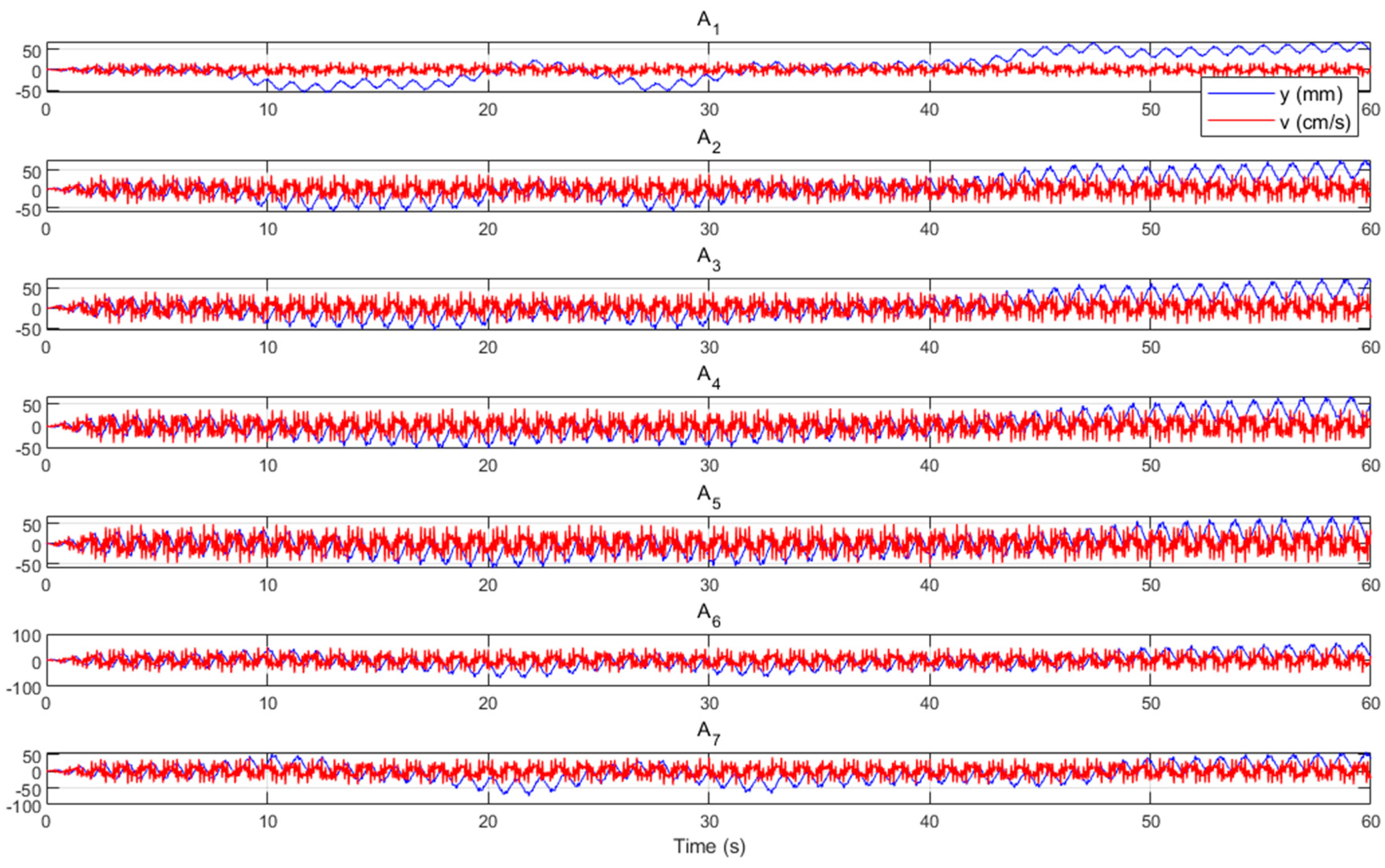
In this section, the CDE-DMD method is used to predict and control the robot’s overall lateral motion. This approach helps capture the gross movements and provides a framework for regulating them effectively. The system, referring to Figure 3, is spatially discretized to seven points, A1 to A7, equally distributed on the midline of the robot’s continuous body. To evaluate the capability of the proposed method in estimating the robot’s gross motion, we first assemble some state data into the Hankel matrix, as presented in (3). The state vector, shown by the complex variable z within this manuscript, includes the lateral position and velocity, which can be obtained by differentiation of the position data.
Different open-loop arbitrary scenarios are considered, where δ 0 = 0.1 and the control input δ takes constant values like
δ 0.1 ,   0 ,   + 0.1
According to (18), when δ = 0.1 , we will have P R = P 1 and P L = 0.9 P 1 . Likewise, when δ = 0.1 , we will have P R = 0.9 P 1 and P L = P 1 , and when δ = 0 , symmetric actuation is provided as P R = P L . One advantage of this input is the feasibility of implementation using standard industrial pneumatic components. A pneumatic regulator can be used to provide P 2 = 0.9 P 1 from a nominal pressure of 600 [KPa]. Switching pneumatic valves, which are smaller and much less expensive than analog pressure control valves, are used to guide the discrete input pressures to the actuators. Next, some data is required to assemble the data matrices and perform the calculations (also known as training within ML terminology). An arbitrary input, shown in Figure 7, was applied to drive the system aimlessly. At this point, any arbitrarily varying input resulting in casual navigation with a rich gross motion effect is sufficient (note that high-frequency inputs may not yield a noticeable gross motion). The system response, i.e., the states of the discrete points on the robot midline, is shown in Figure 8. The position data is exhibiting a noticeable overall motion, in addition to oscillations. The modal decomposition (8) is used to separate the different physics by projecting the data into a modal space. Visualizing the modes’ contributions, also called the reconstruction process, helps reveal how each mode influences the system and allows us to distinguish the underlying physical phenomena.
The modal decomposition results are shown in Figure 9. The linear oscillations, shown by the blue curve, demonstrate the pure undulation, which contains the main drive in the anguilliform locomotion. The gross motion, which is of more interest in this work, is the next major part of the signals and is shown by the black curve. The graphs show that the curve provides a good approximation of the gross motion. Note that the superposition of the linear oscillations and the overall motion results in a form of reduced-order approximation (reconstruction) of the original data. To investigate this issue numerically, the superposition of the linear oscillations and the gross motion is plotted in Figure 10. The graph shows that errors linked to higher modes have smaller amplitudes compared to the main data. This analysis reveals the contribution of modes in the pure undulation, as well as a drift or trend attributed to rigid-body-like motion, namely gross motion of the robot. The results from the CDE DMD predictor, as presented in (16), are illustrated in Figure 11. From the ML perspective, this method processes the data in an unsupervised manner. Specifically, the CDE DMD algorithm extracts the existing modes within the dynamics from the data matrix.
It is important to note that if the data lacks mode information—such as when it is collected from a short, straight motion of the robot in this study—DMD techniques may not be able to identify the modes.
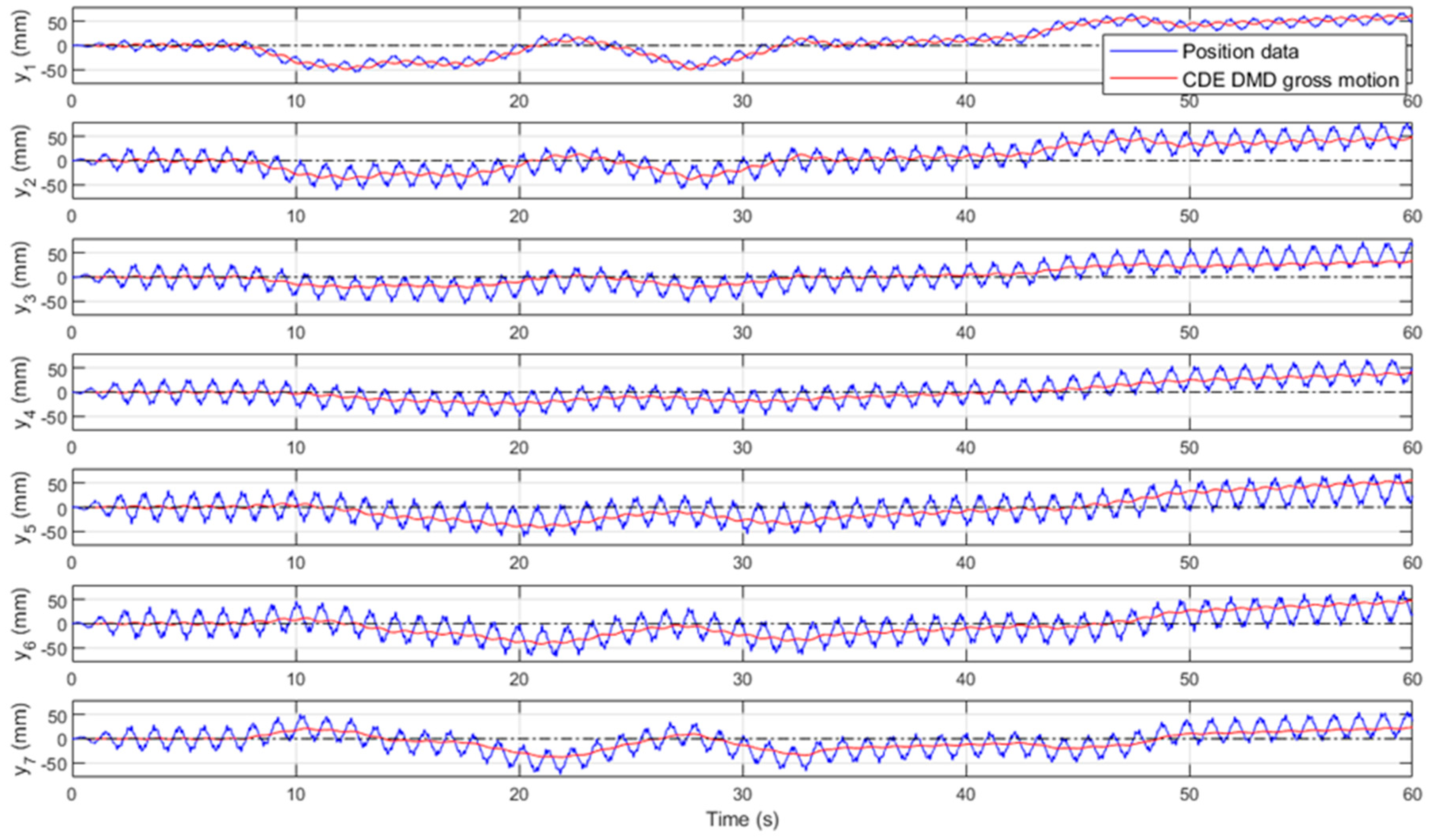
The number of delayed coordinates, d, is chosen to be 110, which, with the sampling time of 0.005 s, is equivalent to half of the undulation period, 1.1s. Similar to the mechanical vibrations, if an input is not rich enough, a mode may not be excited enough to be detected by data-driven model discovery methods. Another interesting topic in the arena of ML is the performance of the algorithm on unseen data. Employing the ML terminology, the previous data (represented in Figure 8) can be seen as the training data. The data was used to measure the hyperparameters of (16). Next, a different maneuvering scenario with the input signal shown in Figure 12 is simulated to evaluate the algorithm’s ability to identify gross motion in previously unseen situations. In this case, the algorithm updates a data window (Figure 2) with the current measurements. Then, the data is used by the pretrained model (16) to predict the trace. The calculated trace is shown as the CDE-DMD gross motion in Figure 13.
For the closed-loop control, the linear gain in (19) is heuristically selected as follows based on the subsequent explanations. As ( z ˜ 4 , m + 1 ) = y 4 corresponds to the position of the middle point (A4), a control term like k 1 ( z ˜ 4 , m + 1 ) is used to make up for the distance error. Additionally, another term is required to react against the orientation error. The angle of the robot orientation can be related to ( z ˜ 1 , m + 1 ) ( z ˜ 7 , m + 1 ) , which corresponds to the position of the distal points, A1 and A7.
Therefore, the controller is expressed as
δ = sgn k 1 ( z ˜ 4 , m + 1 ) + k 2 ( z ˜ 1 , m + 1 ) ( z ˜ 7 , m + 1 ) δ 0
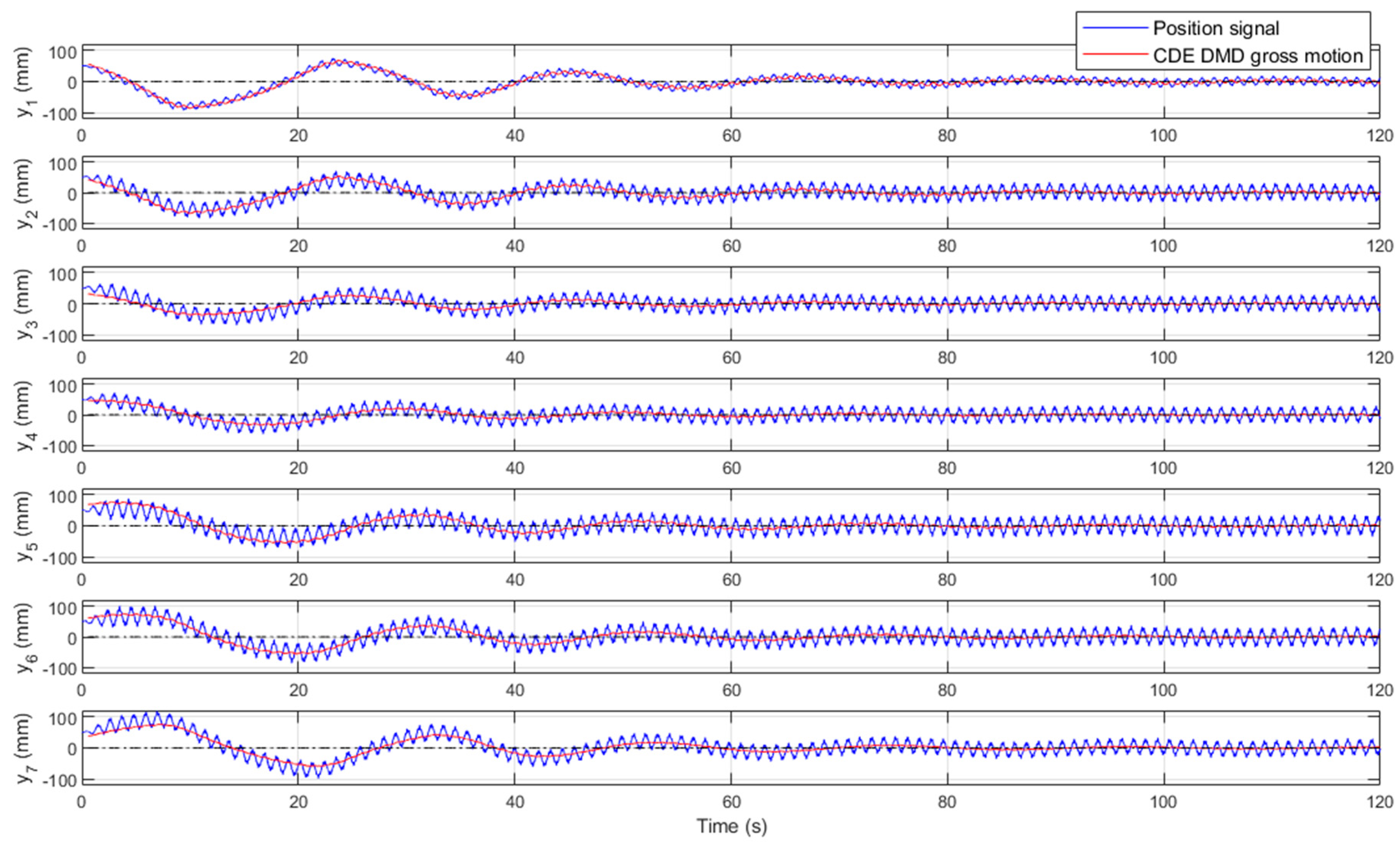
This control can be seen as a simple bioinspired control law [30] for steering right or left. Analogous to the step response in classic control of linear systems, the closed-loop system performance can be demonstrated by considering a non-zero initial condition for the position of the robot. Two examples are considered, where, in the first case, the robot has an angle error, and in second, it has a distance error with respect to the desired line. Simulation results for the open-loop system response are illustrated in Figure 14. The response of the closed-loop system using (21) with k 1 = 50 and k 2 = 330 is given in Figure 15 and Figure 16. Note that the oscillation around the zero (shown by the dashed line) is the desired objective because it represents swimming on the line. However, when the robot has a non-zero initial angle to the line, the initial position of the discrete points will have a non-zero initial value. As can be seen in Figure 15, the controller compensates for this error. Similarly, in the closed-loop scenario, shown in Figure 16, an initial distance error relative to the zero line is considered. The results show that the controller provides the error zeroing necessary for navigation on the desired line. The value of the initial state, which was called the initial error, can also be interpreted as setpoint change in classical control. Therefore, the controller can be extended for navigation of the robot. Suppose the setpoint (which is the desired direction line) is described by angle θ and a distance β respect to zero line. The controller (21) can incorporate the setpoint data (which can be given by a joystick, for example), as in
δ = sgn k 1 ( z ˜ 4 , m + 1 ) β + k 2 ( z ˜ 1 , m + 1 ) ( z ˜ 7 , m + 1 ) θ γ δ 0
The robot path can likewise be described with interconnected piecewise lines that deliver the setpoint changes. Nevertheless, extension of the controller for more complex navigation is not within the focus of this article and remains for future investigations.

4. Discussion

Modeling a soft swimming robot for model-based control is a formidable task. Therefore, this study proposes a data-driven control method based on FSI simulation data. Various open-loop and closed-loop scenarios were analyzed to assess the capability of the CDE DMD method in predicting the robot’s gross motion. This analysis aimed to determine how effectively the method can forecast large-scale motion patterns under different control conditions. Within fish locomotion studies, the ability to swim in a straight line is known as directional stability.
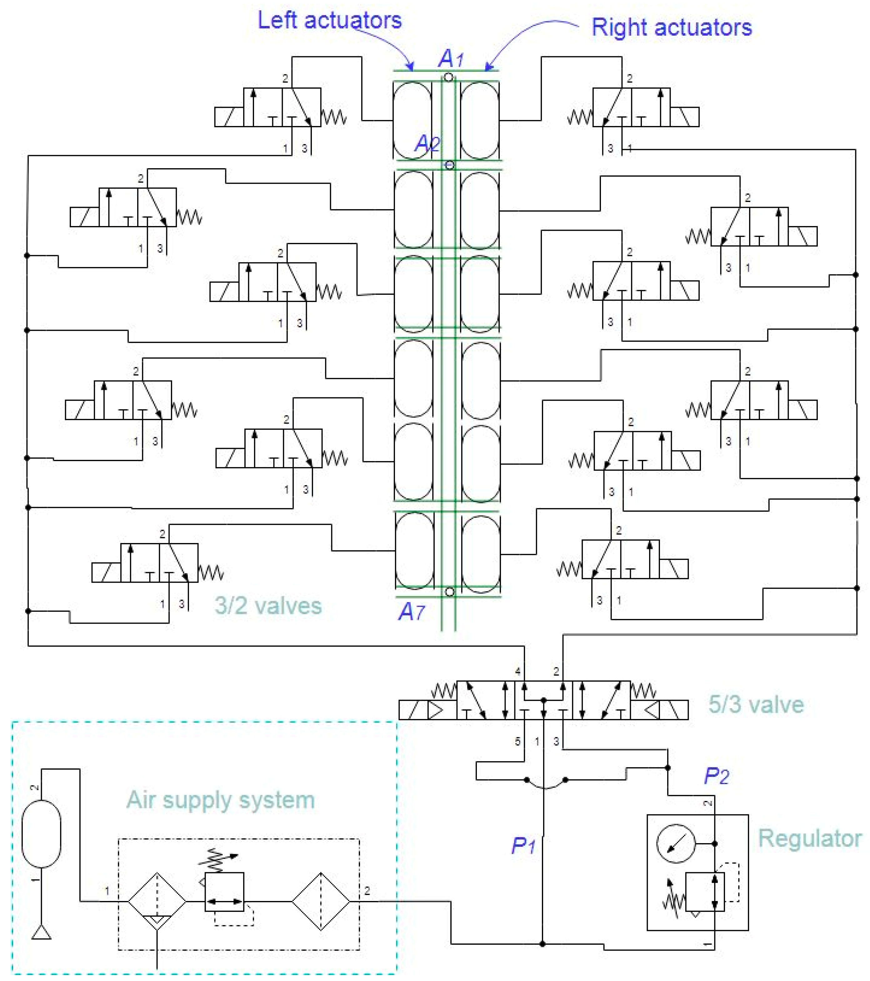
In comparison with robotics terminology, the directional stability can be related to trajectory following, with the difference that the desired trajectory is a straight line, and conceptually, less position error is expected. In robot path following, regular shapes such as squares or circles are commonly used as desired paths. The robot is then controlled to approximately follow these paths, allowing for generally tolerable position errors. Furthermore, unlike sharp turns, which represent transient curling behavior, directional stability is linked to steady swimming. The proposed control is implemented through small pressure adjustments, using the pneumatic system, schematically shown in Figure 17. The robot is depicted schematically, with pneumatic components represented by standard symbols. Each segment is actuated by two 3/2 valves, allowing it to bend either to the right or left. The 3/2 valves are controlled by the sequential signal given in Figure 5. The directional control is performed by the 5/3 valve, which provides the pressure for the 3/2 valves related to each side of the robot.
An air supply delivers the nominal pressure, P1, and a regulator provides the P2 pressure for the direction control. The control rule given in (21) is shown as the control signal to the 5/3 valve. The three-digit values are to select one of the three possible states of the valve using the solenoids. The simulation results indicate that the controller generates regulating signals that are practically feasible for hardware implementation. With an initial pose error, the controller settles the error after approximately 60 s. The prediction rule acts as a data-driven observer for tracing the robot. Open-loop simulations show that the prediction can be used to generate a trace that approximates the robot’s overall trajectory. In soft robots and natural anguilliform swimmers, in contrast to rigid robots, which can rely on joint sensors, positioning and tracking the swimmer is complex. The proposed algorithm may be used for tracking or positioning purposes (with or without control). The algorithm is highly compatible with real-time application and microcontroller implementation. As the prediction model (16) and the controller (21) provide a linear map between the current measurement values and the system input, the calculation effort is minimal. A calculation limitation is the time of the embedded delay.
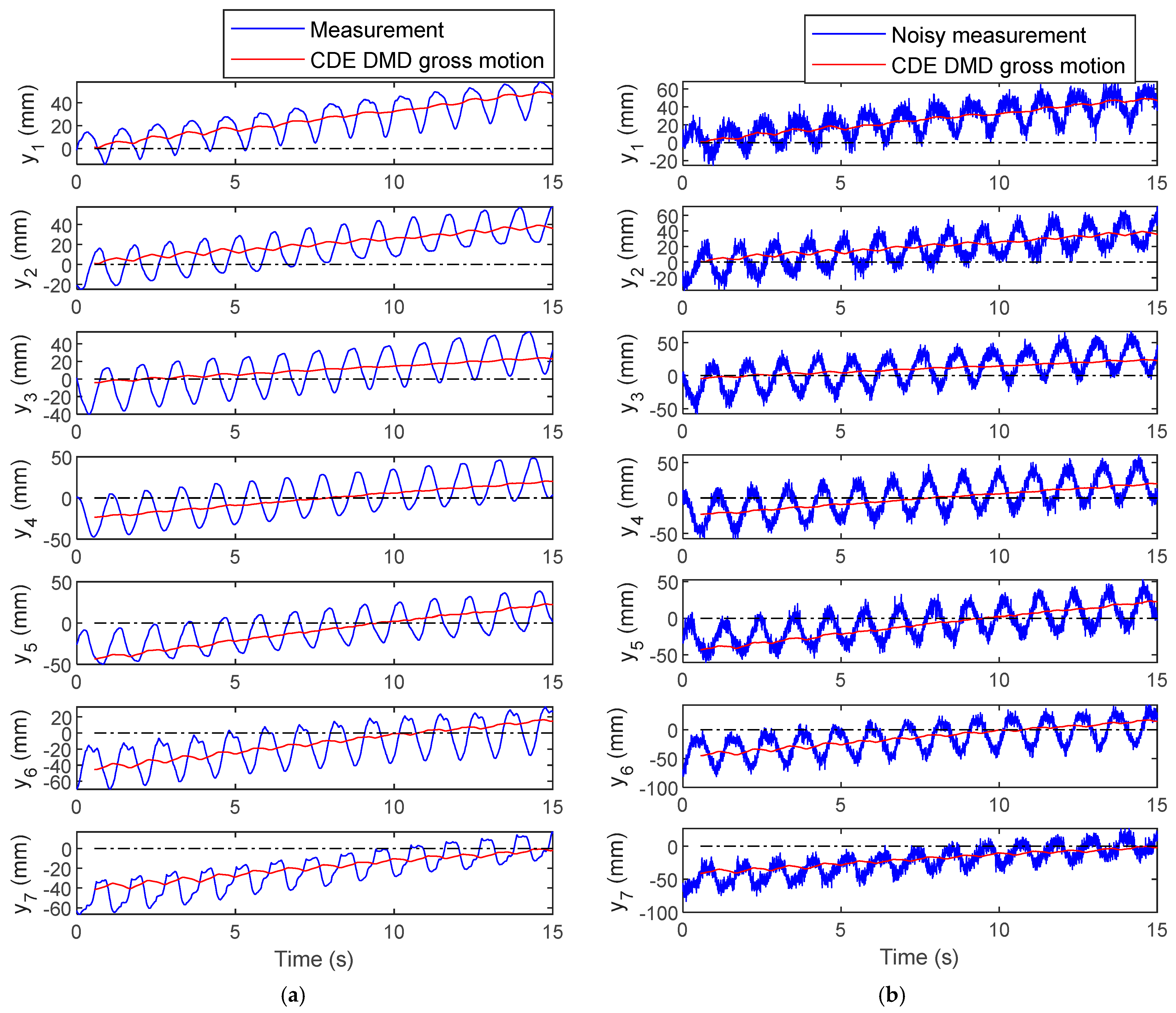
Delay embedding means that some previous measurements are to be known and saved in the computer. This is the reason why the graphs representing CDE DMD gross motion do not start from the zero time. In order to evaluate the prediction method, some open-loop experimental data were analyzed. The robot swims with a small angle in a short water tank (as in [21]). The collected data is used as the ground truth in the CDE DMD prediction model.
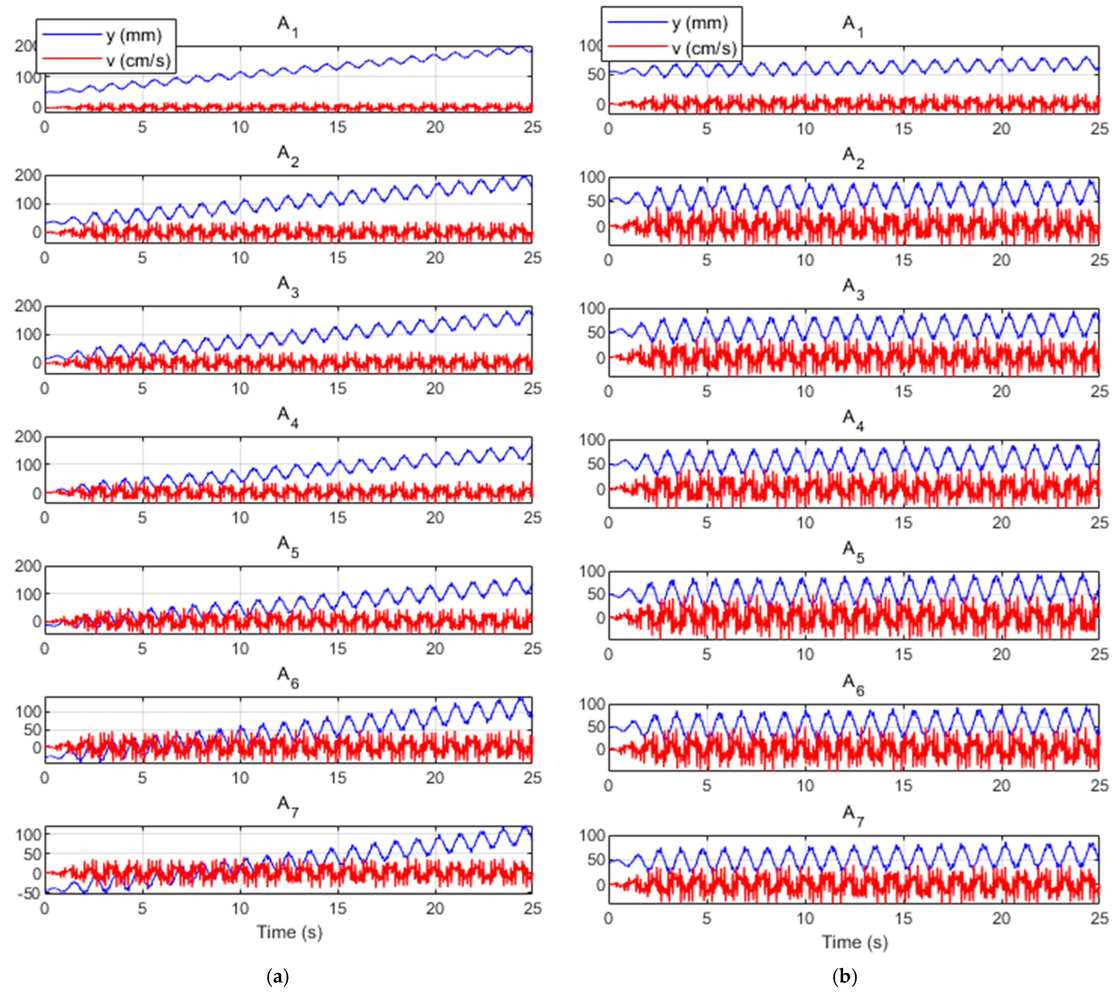
Additionally, some artificial noise is added to the measurements to check the performance against random noise. The prediction results over the measured signals are illustrated in Figure 18. Note that the algorithm treats the signals in an online manner and draws the gross motion trend, without access to the whole dataset. At this point, it is interesting to discuss the treatment of disturbances, noise, and practical limitations within the experimental setup. The main control problems in swimming robots (and generally in mobile robots, in contrast to manipulators) include problems related to navigation. Anguilliform swimming of soft robots involves complex hydrodynamics that influence motion and deformation of the compliant body. The previous studies have shown a variety of interacting FSI modes, including the main undulation modes and chaotic modes. Such modes may be seen as disturbances within a classic control loop.
In fact, an initial motivation of this study was to develop a modal control strategy that isolates the gross motion dynamics and control it like a rigid body motion mode. This article implicitly suggests that imperfectness effects like disturbances may eradicate directional stability, and so closed-loop control is required. The step-response-like simulation reflects the performance of the controller after a setpoint variation. This variation might be due to a disturbance exerted as an unpredicted fluid motion.
An advantage of the proposed method is that random and high-frequency noise is cancelled out, as it is not projected on the dominant modes. In Figure 18b, Gaussian white noise with zero mean and a standard deviation of 6 was added to the measured signals (Figure 18a) using MATLAB® R2022b (MathWorks®, Natick, MA, USA). This work paves a road for further development of the robot and implementation of closed-loop control. For closed-loop control, some practical hardware improvement is also required. The main challenges include the use of real-time measurement sensors and an experiment pool that allows the robot to swim for a sufficiently long time or distance. These challenges are the actual limitations of the soft robot and should be addressed in future work. The robot was primarily designed for research purposes and is powered using pneumatic pipes. Therefore, the robot cannot swim far distances due to the pipes’ length limitation (plus the pool length). However, a self-powered version of the robot (for example, with pumps) is required to serve as a field robot. On the other hand, the optical tracking system has limitations in real-time application and in-field situations. Suitable sensors should be integrated in the control system to enable real-time measurement, outdoor positioning, and perhaps wireless communication. The future research directions can include the development of the hardware system to alleviate such limitations.

5. Conclusions

In this paper, we propose a data-driven method for prediction of the direction and control of an anguilliform swimming soft pneumatic robot. First, the problem of directional stability, a concept borrowed from fish locomotion, was explained, and an actuation hypothesis was discussed using COMSOL Multiphysics® 6.2 simulations. We adopted a bionic approach, where the control problem is viewed as directional stability inspired by the two separate navigation behaviors of fish: curling and stable swimming, characterized by asymmetric actuation forces. We proposed a DMD-based algorithm to predict the swimmer’s gross motion, which is then used for closed-loop control in the simulations. The results show that the proposed method, namely, CDE DMD, reveals the trend line associated with the robot’s gross motion, with both training and unseen datasets. Furthermore, a heuristic controller was proposed based on the prediction model. It was concluded that a slight discrepancy between the maximum forces on the lateral sides generates asymmetric material movements that can be exploited to achieve directional stability in anguilliform swimming using the CDE DMD method. This paper proposes techniques to improve the path-following performance of soft pneumatic robots in aquatic navigations. These findings are particularly significant for long-distance operations of untethered anguilliform swimming robots, while sharp curling for local navigation remains a topic for future research.

Author Contributions

Conceptualization, M.S. and H.W.; methodology, M.S.; software, M.S.; validation, M.S. and H.W.; formal analysis, M.S.; investigation, M.S. and H.W.; resources, M.S. and H.W.; data curation, M.S. and H.W.; writing—original draft preparation, M.S.; writing—review and editing, H.W.; visualization, M.S.; supervision, H.W.; project administration, M.S. and H.W.; funding acquisition, H.W. All authors have read and agreed to the published version of the manuscript.

Funding

This research received no external funding.

Institutional Review Board Statement

Not applicable.

Informed Consent Statement

Not applicable.

Data Availability Statement

The original contributions presented in this study are included in the article; further inquiries can be directed to the corresponding author.

Conflicts of Interest

The authors declare no conflicts of interest.

Abbreviations

The following abbreviations are used in this manuscript:
ALEArbitrary Lagrangian–Eulerian
CDEComplex-variable Delay Embedding
CFDComputational Fluid Dynamics
DMDDynamic Mode Decomposition
FEFinite Elements
FPTFluid-Particle Tracing
FSIFluid–Structure Interaction
MLMachine Learning
ReReynolds Number
SPFSingle-Phase Flow
SVDSingular Value Decomposition

References

  1. Sfakiotakis, M.; Lane, D.M.; Davies, J.B.C. Review of fish swimming modes for aquatic locomotion. IEEE J. Ocean. Eng. 2002, 24, 237–252. [Google Scholar] [CrossRef]
  2. Lindsey, C.C. Form, function, and locomotory habits in fish. In Fish physiology; Elsevier: Amsterdam, The Netherlands, 1978; Volume 7, pp. 1–100. [Google Scholar]
  3. Satoi, D.; Hagiwara, M.; Uemoto, A.; Nakadai, H.; Hoshino, J. Unified motion planner for fishes with various swimming styles. ACM Trans. Graph. 2016, 35, 1–15. [Google Scholar] [CrossRef]
  4. Hasib, S.A.; Gulzar, M.M.; Oishy, S.R.; Maaruf, M.; Habib, S.; Shakoor, A. An investigation of innovative strategies in underwater soft robotics. Eng. Sci. Technol. Int. J. 2025, 70, 102123. [Google Scholar] [CrossRef]
  5. Mathew, A.T.; Feliu-Talegon, D.; Abdullahi Adamu, Y.; Ben Hmida, I.; Armanini, C.; Stefanini, C.; Seneviratne, L.; Renda, F. Zodiaq: An isotropic flagella-inspired soft underwater drone for safe marine exploration. Soft Robot. 2025, 12, 410–422. [Google Scholar] [CrossRef]
  6. Ma, H.; Zhou, J.; Yeow, R. Soft Robotic Snake with Tunable Undulatory Gait for Efficient Underwater Locomotion. Adv. Robot. Res. 2025, 0, e2500061. [Google Scholar] [CrossRef]
  7. Alexandris, C.; Papageorgas, P.; Piromalis, D. Positioning systems for unmanned underwater vehicles: A comprehensive review. Appl. Sci. 2024, 14, 9671. [Google Scholar] [CrossRef]
  8. Tytell, E.D.; Lauder, G.V. The hydrodynamics of eel swimming: I. Wake structure. J. Exp. Biol. 2004, 207, 1825–1841. [Google Scholar] [CrossRef] [PubMed]
  9. Gregorio, E.; Godoy-Diana, R.; Herrel, A. Turning without Fins: How Snakes Achieve High Maneuverability While Swimming. 2025. HAL Preprints 2025. hal-04876557. Available online: https://hal.archives-ouvertes.fr/hal-04876557 (accessed on 11 September 2025).
  10. Yu, L.; Lai, J.; Huang, J.; Liu, H.; Pi, X. Wireless motion control of a swimming eel-machine hybrid robot. Bioinspir. Biomim. 2025, 20, 036010. [Google Scholar] [CrossRef]
  11. Xu, J.-X.; Niu, X.-L.; Ren, Q.-Y.; Wang, Q.-G. Collision-free motion planning for an Anguilliform robotic fish. In Proceedings of the 2012 IEEE International Symposium on Industrial Electronics, Hangzhou, China, 28–31 May 2012; pp. 1268–1273. [Google Scholar]
  12. Melsaac, K.; Ostrowski, J.P. A geometric approach to anguilliform locomotion: Modelling of an underwater eel robot. In Proceedings of the IEEE International Conference on Robotics and Automation, Detroit, MI, USA, 10–15 May 1999; pp. 2843–2848. [Google Scholar]
  13. Raj, A.; Kumar, A.; Thakur, A. Automated locomotion parameter tuning for an anguilliform-inspired robot. In Proceedings of the 2016 IEEE International Conference on Systems, Man, and Cybernetics (SMC), Budapest, Hungary, 9–12 October 2016; pp. 002564–002569. [Google Scholar]
  14. Thati, S.K.; Raj, A.; Thakur, A. Optimal and Dynamically Feasible Path Planning for an Anguilliform Fish-Inspired Robot in Presence of Obstacles. In Proceedings of the ASME International Design Engineering Technical Conferences and Computers and Information in Engineering Conference, Quebec, QC, Canada, 26–29 August 2018. [Google Scholar]
  15. Niu, X.; Xu, J.; Ren, Q.; Wang, Q. Locomotion generation and motion library design for an anguilliform robotic fish. J. Bionic Eng. 2013, 10, 251–264. [Google Scholar] [CrossRef]
  16. Yu, F.; Wu, Z.; Wang, J.; Yu, L.; Feng, Y.; Tan, M.; Yu, J. Learning From Fish: A Two-Stage Transfer Learning Method for a Bionic Robotic Fish. IEEE Trans. Autom. Sci. Eng. 2025, 22, 18796–18808. [Google Scholar] [CrossRef]
  17. Shi, H.; Meng, Y.; Cui, W.; Rao, M.; Wang, S.; Xie, Y. Biomimetic Underwater Soft Snake Robot: Self-Motion Sensing and Online Gait Control. IEEE Trans. Robot. 2025, 41, 1193–1210. [Google Scholar] [CrossRef]
  18. He, J.; Wu, C.; Li, Q.; Cui, Y. Efficient anguilliform swimming simulations via coupled overset mesh and RBF mesh deformation techniques. Arch. Appl. Mech. 2025, 95, 104. [Google Scholar] [CrossRef]
  19. Huang, X.-T.; Sun, P.-N.; Lyu, H.-G.; Zhong, S.-Y. Study of 3D self-propulsive fish swimming using the δ+-SPH model. Acta Mech. Sin. 2023, 39, 722053. [Google Scholar] [CrossRef]
  20. Wu, T.Y.-T. Hydromechanics of swimming propulsion. Part 1. Swimming of a two-dimensional flexible plate at variable forward speeds in an inviscid fluid. J. Fluid Mech. 1971, 46, 337–355. [Google Scholar] [CrossRef]
  21. Sayahkarajy, M.; Witte, H. Analysis of Robot–Environment Interaction Modes in Anguilliform Locomotion of a New Soft Eel Robot. Actuators 2024, 13, 406. [Google Scholar] [CrossRef]
  22. Sayahkarajy, M.; Witte, H. Temporal Evolution of the Hydrodynamics of a Swimming Eel Robot Using Sparse Identification: SINDy-DMD. J 2025, 8, 2. [Google Scholar] [CrossRef]
  23. Schmid, P.J. Application of the dynamic mode decomposition to experimental data. Exp. Fluids 2011, 50, 1123–1130. [Google Scholar] [CrossRef]
  24. Duke, D.; Soria, J.; Honnery, D. An error analysis of the dynamic mode decomposition. Exp. Fluids 2012, 52, 529–542. [Google Scholar] [CrossRef]
  25. Colbrook, M.J.; Drysdale, C.; Horning, A. Rigged dynamic mode decomposition: Data-driven generalized eigenfunction decompositions for Koopman operators. SIAM J. Appl. Dyn. Syst. 2025, 24, 1150–1190. [Google Scholar] [CrossRef]
  26. Chávez-Dorado, J.; Scherl, I.; DiBenedetto, M. Wave and turbulence separation using dynamic mode decomposition. J. Atmos. Ocean. Technol. 2025, 42, 509–526. [Google Scholar] [CrossRef]
  27. Asada, H.; Kawai, S. Exact parallelized dynamic mode decomposition with Hankel matrix for large-scale flow data. Theor. Comput. Fluid Dyn. 2025, 39, 8. [Google Scholar] [CrossRef]
  28. Sayahkarajy, M.; Witte, H. Empirical Data-Driven Linear Model of a Swimming Robot Using the Complex Delay-Embedding DMD Technique. Biomimetics 2025, 10, 60. [Google Scholar] [CrossRef] [PubMed]
  29. Zhao, X.; Ye, B. Similarity of signal processing effect between Hankel matrix-based SVD and wavelet transform and its mechanism analysis. Mech. Syst. Signal Process. 2009, 23, 1062–1075. [Google Scholar] [CrossRef]
  30. Wang, J.; Chen, H. BSAS: Beetle swarm antennae search algorithm for optimization problems. arXiv 2018, arXiv:1807.10470. [Google Scholar] [CrossRef]
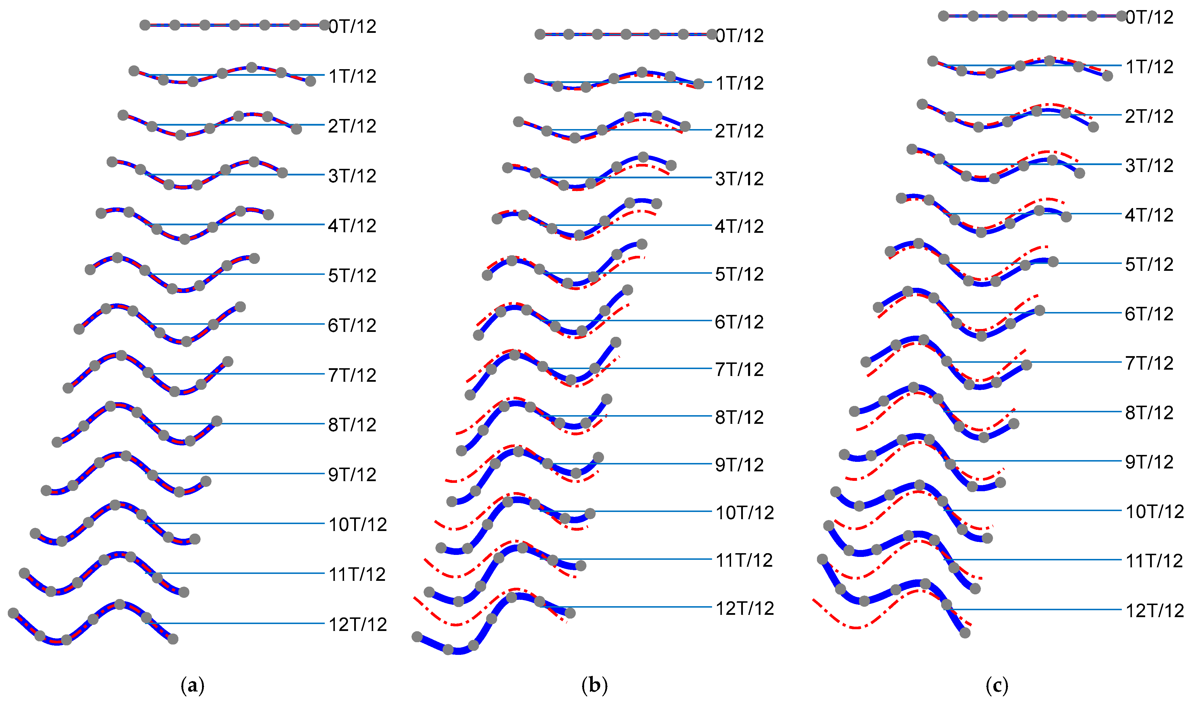
Figure 1. Illustration of anguilliform swimming kinematics within an undulation period, T: (a) motion in a straight line; (b) swimming with left-tilting tendency; (c) right-tilting motion. The blue line represents the initial state, and the dashed-dot represents the (desired) position in straight motion.
Applsci 15 10045 g001
Figure 2. Memory stacking to update h , m d .
Applsci 15 10045 g002
Figure 3. The robot model: (a) three-dimensional view; (b) model of the backbone; (c) the finite element mesh, dimensions, and forces. The dimensions are given in mm, and red arrows represent the actuator forces on the backbone. The small blue circles represent motion-tracking points from the head (A1) to the distal segment (A7).
Applsci 15 10045 g003
Figure 4. The underlying mathematical model of the swimming robot.
Applsci 15 10045 g004
Figure 5. The segmental actuation sequence with period T = 1.1 s.
Applsci 15 10045 g005
Figure 6. The FPT analysis: (a) the initial state of the particles on the mesh; (b) simulation results with asymmetric actuation δ = 0.1 ; (c) symmetric actuation; (d) asymmetric actuation with δ = + 0.1 . The color bar represents the particle indices, and the FPT results are shown at t = 10 T.
Applsci 15 10045 g006
Figure 7. The arbitrary input in the training scenario.
Applsci 15 10045 g007
Figure 8. The lateral position and velocity data of the tracking points, A1 to A7.
Applsci 15 10045 g008
Figure 9. Decomposition of the position data into the linear oscillations and the gross motion.
Applsci 15 10045 g009
Figure 10. Reconstruction of the data with the main modes and the reconstruction error.
Applsci 15 10045 g010
Figure 11. Results of the CDE DMD gross motion prediction (training scenario).
Applsci 15 10045 g011
Figure 12. Arbitrary input in the unseen scenario.
Applsci 15 10045 g012
Figure 13. Results of the CDE DMD gross motion prediction for the unseen scenario.
Applsci 15 10045 g013
Figure 14. System response without the control: (a) for initial orientation error; (b) for pure dislocation initial error.
Applsci 15 10045 g014
Figure 15. A closed-loop scenario of CDE DMD control with a non-zero initial orientation.
Applsci 15 10045 g015
Figure 16. A closed-loop scenario with an initial dislocation.
Applsci 15 10045 g016
Figure 17. Schematic of the pneumatic control system.
Applsci 15 10045 g017
Figure 18. Implementation of the CDE DMD prediction on open-loop experiment data: (a) measured signals; (b) noise-added signals.
Applsci 15 10045 g018
Table 1. The pseudocode of the online prediction and control algorithm.
% Initialization 1:
for n = d:−1:0% for loop from d to 0 by step −1
Measure z% current state vector z is measured
zm_past(n) z %   zm ( n )   is   representing   z , m n
Delay   Δ t
end
while (true) % while loop (main code)
Measure z% current state vector z is measured
%   here   h , m d is updated:
zm(0)  z
for n = 1:1:d
zm(n)  zm_past(n − 1)
zm_past(n − 1)  zm(n − 1)
end
% Future gross motion:
Calculate   z ˜ , m + 1 % use (16)
% Controller update
Calculate δ and pressure% use (19) and (18)
Apply the pressure to the system (simulation/experimental model)
Delay   Δ t
end
1 Comments are indicated by %.
Disclaimer/Publisher’s Note: The statements, opinions and data contained in all publications are solely those of the individual author(s) and contributor(s) and not of MDPI and/or the editor(s). MDPI and/or the editor(s) disclaim responsibility for any injury to people or property resulting from any ideas, methods, instructions or products referred to in the content.