Integration of Peridynamics and Deep Learning for Efficient and Accurate Thermomechanical Modeling

Highlights

What are the main findings?

• A novel hybrid model (PD-DL) that combines peridynamics (PD) and deep learning (DL) was developed for rapid failure prediction;
• The established PD thermomechanical model was validated with high accuracy, showing errors below 0.7% compared to the finite element method (FEM);
• The developed deep learning surrogate model achieves a 1200-fold speedup in prediction compared to the pure PD computation.

What is the implication of the main finding?

• The PD-DL framework provides an efficient and accurate computational solution for real-time failure analysis in complex thermomechanical scenarios;
• The significant computational acceleration makes this model highly promising for practi-cal engineering applications, such as digital twins and real-time health monitoring and prognosis.

Abstract

Accurate and efficient modeling of thermomechanical failure in critical structures under extreme conditions remains a great challenge. Traditional local methods struggle with discontinuities, such as fractures, while peridynamics (PD) is computationally intensive. This study presents a rapid prediction framework that combines sequential PD thermomechanical coupling simulations with a deep learning (DL) surrogate model. The framework adopts bond-based PD to solve the deformation field, accounting for thermal expansion, whereas the temperature field is handled using the peridynamic differential operator to address boundary effects and enhance transient accuracy. The validation results show that the PD thermomechanical coupling model achieved high accuracy. For example, the cooling simulation results of a 2D plate using PD and FEM show that the results had a global error in temperature and displacement of less than 0.7%. In the Al₂O₃ ceramic quenching simulations, the crack propagation path is accurately reproduced using the PD model, which matches the experimental data well. To improve the computational efficiency, the DL surrogate model was trained on a large dataset generated by PD simulations. The inputs include the crack geometries and loads, and the outputs are the predicted crack openings, average radial displacement/strain, and circumference change rates. The optimized deep neural network (DNN) consisted of two hidden layers, each with nine neurons. The DNN model predicted complex multi-output responses in approximately 0.5 s, about 1200 times faster than direct PD simulation, maintaining high accuracy. The PD-DL framework offers a new direction for assessing the thermomechanical damage and structural integrity in engineering applications.

1. Introduction

Reactor pressure vessels (RPV) [1], aerospace propulsion chambers [2], and other critical pressure-bearing structures play a crucial role in the energy and aerospace sectors. During normal operation, these structures are subjected to high temperatures, high pressures, and other complex loading conditions for prolonged periods. This exposure can lead to thermal stress concentration, thermal cracking, and other deformation-related damage [3]. Such phenomena can result in localized failure or even complete structural collapse, which poses a significant risk to the safety and operational lifespan of engineering equipment. Therefore, it is essential to develop efficient and accurate computational methods for analyzing the deformation and damage behavior of these structures under thermomechanical coupling.

Over the past few decades, numerical methods based on classical continuum mechanics theory, such as the finite element method (FEM) [4] and finite difference method [5], have been the mainstream tools in thermomechanical coupling analysis. However, these methods are limited by their continuity assumptions when dealing with discontinuous deformation problems, such as damage, fracture, and crack propagation, making it difficult to describe crack initiation and evolution naturally. In complex scenarios involving large deformations, strong nonlinearity, and multiphysics coupling, these methods often encounter difficulties with convergence and exhibit strong mesh dependency, limiting their applicability in simulating complex failure behaviors [6]. Therefore, in recent years, methods such as the smoothed particle hydrodynamics [7,8], the moving least square method [9,10], the phase-field method [11,12], and peridynamics (PD) [13,14], which are based on meshless or particle-based numerical methods, have gradually been introduced.

The PD theory, proposed by Silling in 2000 [15], is a nonlocal continuum mechanics theory based on spatial integral equations. It replaces partial differential equations with integral equations, enabling the consideration of nonlocal effects, which is particularly useful for simulating crack propagation and material damage [16,17,18]. Recently, some researchers have attempted to introduce the PD method into thermomechanical coupling models. Oterkus et al. [19] derived a fully coupled PD thermodynamic equation based on thermodynamic principles, proposing a generalized model combining energy conservation and free energy functions to solve complex thermomechanical coupling problems. Wang et al. [20,21] proposed a bond-based peridynamic (BBPD) thermomechanical coupling PD model and validated its accuracy through benchmark problems. To study thermal failure in functionally graded materials, He et al. [22] proposed an improved fully coupled thermomechanical ordinary state-based PD model to study thermal failure in functionally graded materials, and analyzed the effect of material gradient changes on the thermal response by introducing an exothermic term due to irreversible damage. Yang et al. [23] proposed a fully coupled thermomechanical PD model for simulating the thermomechanical response and thermal-induced fracture of solids. Additionally, PD-based thermomechanical coupling models have been used to address issues such as thermal damage to railway rails [24], high temperature fractures of alloys [25], and frost heaving in rocks [26]. In summary, the PD method demonstrates unique advantages in handling nonlocal effects under thermomechanical loads, particularly in simulating complex thermomechanical coupling processes, such as local damage and crack propagation.

Despite the substantial promise of PD and related nonlocal formulations for characterizing thermomechanically coupled damage evolution, their intrinsic nonlocality makes them significantly more computationally expensive than classical local continuum approaches. The response of each material point must be evaluated by integrating over its neighborhood, which renders PD simulations—particularly those involving long-duration physical evolution—computationally intensive and time-consuming [27,28]. This high computational cost severely constrains the use of PD in real-time engineering analysis and rapid prediction, for example in the fast diagnosis of sudden failures, large-scale parametric screening, and online feedback within digital-twin systems. It is therefore imperative to develop a computational framework that preserves the high accuracy of PD while satisfying real-time performance requirements. Deep learning (DL) offers a transformative pathway to address this tension [29,30].

Through training, DL models can learn highly nonlinear mappings from input parameters to complex physical responses, thereby serving as efficient surrogate models [31]. Once trained, neural networks deliver extremely fast forward predictions, typically within milliseconds to seconds, accomplishing tasks that would require hours or even days with traditional numerical solvers, thus resolving the timeliness bottleneck. Building on this insight, the present work integrates the high-fidelity modeling capability of PD with the rapid inference of DL to construct a PD–DL hybrid framework. High-fidelity data generated by PD simulations are used to train the neural networks, which are then employed for fast prediction. This approach not only remedies the computational inefficiency of pure PD, but also mitigates the potential distortions of purely data-driven methods by embedding physics-based information, thereby enabling the accurate, real-time analysis of thermomechanically coupled damage processes.

The remainder of this paper is organized as follows. Section 2 presents a sequential thermomechanical coupling model based on PD. Section 3 validates the accuracy of the proposed thermomechanical coupling model for damage and deformation response calculations using two typical examples. Section 4 discusses the method of constructing a neural network model based on PD simulation data and establishes an efficient neural network model for fast prediction in thermomechanical coupling analysis.

2. Construction of PD Thermomechanical Coupling Model

The thermomechanical coupling model established in this study uses a sequential coupling approach. The deformation field was calculated using the BBPD model, which is the most widely used PD model. Its modeling concept is intuitive, clear, and easy to implement, and forms the basis of state-based PD (SBPD) modeling research. The temperature field was calculated using the peridynamic differential operator (PDDO) [32], which offers significant improvements over traditional BBPD and SBPD heat conduction models in handling complex boundary conditions and transient heat transfer under extreme conditions [33].

2.1. Motion Equations in BBPD

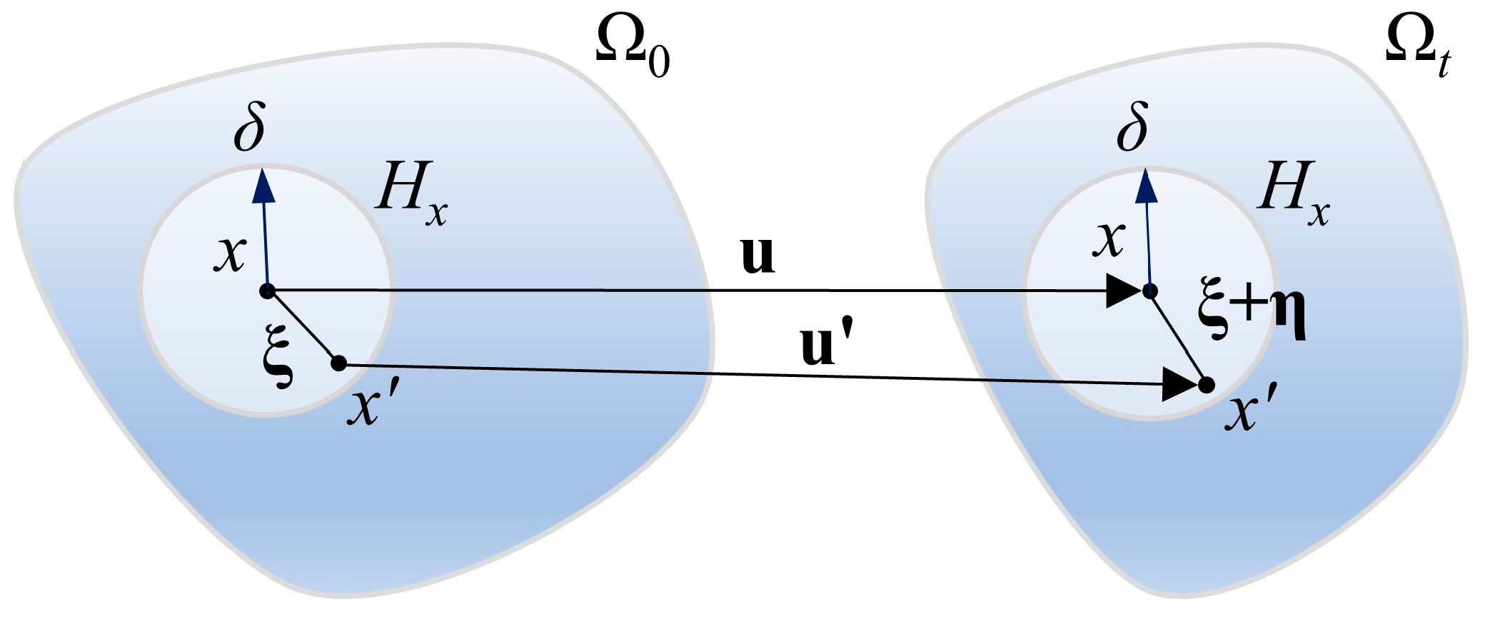
Based on the PD theory, the research domain Ω is discretized into a finite number of material points, each containing physical material information. As shown in Figure 1, within the interaction range H_x of any material point x, there exists another material point x’, and these two material points interact in the form of a “bond.” At the initial time, the position vectors of material points x and x’ are denoted as x and x’, respectively, and the relative position vector between the two material points is ξ = x’ − x. At any time t, the position vectors of material points x and x’ are denoted as y and y’, respectively. At this time, the displacement vectors of material points x and x’ are u = y − x and u’ = y’ − x’, respectively. The relative displacement vector is η = u’ − u. The equation of motion for material point x at time t can be expressed as

$$\rho \ddot{u}\left(x,t\right)={\displaystyle {\int }_{H_x}f\left(\eta ,\xi ,t\right)\mathrm{d}{V}_{x^{\prime }}}+b\left(x,t\right),$$

(1)

where ρ is the material density and $\ddot{u}$ is the acceleration of material point x at time t. f is the bond force density function, and b is the body force density.

Constructing the bond force density function f is crucial for BBPD modeling. Silling et al. [14] proposed the classical prototype microelastic brittle (PMB) model, which is suitable for homogeneous, isotropic, elastic–brittle materials. In this model, the bond force density function, considering the effects of thermal deformation, can be defined as

$$f\left(\xi ,\eta \right)=\chi c\left(s-\alpha T_{\mathrm{avg}}\right){\displaystyle \frac{\xi +\eta }{\left|\xi +\eta \right|}},$$

(2)

where T_avg represents the change in the average temperature between material points x and x’, α is the coefficient of thermal expansion, and c is the microelastic modulus, which is expressed as follows:

$$c=\left\{\begin{array}{ll}{\displaystyle \frac{6E}{\pi {\delta }^4\left(1-2\nu \right)}}\hfill & 3\mathrm{D}\hfill \\ {\displaystyle \frac{6E}{\pi {\delta }^{3}h\left(1-2\nu \right)\left(1+\nu \right)}}\hfill & \mathrm{plane} \mathrm{strain}\hfill \\ {\displaystyle \frac{6E}{\pi {\delta }^{3}h\left(1-\nu \right)}}\hfill & \mathrm{plane} \mathrm{stress}\hfill \end{array}\right.,$$

(3)

where E is the elastic modulus, v is Poisson’s ratio, and h is the thickness.

χ(ξ,t) is a scalar function that characterizes bond damage, and its expression is given by

$$\chi \left(\xi ,t\right)=\left\{\begin{array}{c}1 s-\alpha T_{\mathrm{avg}}\le s_0\\ 0 s-\alpha T_{\mathrm{avg}}<s_0\end{array}\right.,$$

(4)

$s={\displaystyle \frac{\left|\xi +\eta \right|-\left|\xi \right|}{\left|\xi \right|}}$ is the stretch of the bond between material points. $s_0$ is the critical stretch of the bond, which is related to the fracture energy release rate G_F, and its expression is given by

$$s_0=\left\{\begin{array}{ll}\sqrt{{\displaystyle \frac{10G_F}{\pi c{\delta }^5}}}\hfill & 3\mathrm{D}\hfill \\ \sqrt{{\displaystyle \frac{4G_F}{hc{\delta }^4}}}\hfill & 2\mathrm{D}\hfill \end{array}\right..$$

(5)

Furthermore, the damage function φ(x,t) of material point x can be determined by the ratio of the number of broken bonds to the total number of bonds.

$$\phi \left(x,t\right)=1-{\displaystyle \frac{{\displaystyle {\int }_{H_x}\chi \left(\xi ,t\right)\mathrm{d}{V}_{x^{\prime }}}}{{\displaystyle {\int }_{H_x}1\mathrm{d}{V}_{x^{\prime }}}}}.$$

(6)

2.2. Thermal Conduction Equation Using PDDO

According to Fourier’s law of heat conduction, heat flow always transfers from regions of high temperature to regions of low temperature. The temperature difference drives the heat flow, and the amount of heat passing through a unit cross-section per unit of time is proportional to the temperature gradient

$$q\left(x,t\right)=-k_{\mathrm{T}}\nabla T(x,t),$$

(7)

where q represents the heat flux density. x denotes the position vector, k_T is the thermal conductivity coefficient, T is the temperature, and $\nabla$ denotes the gradient operator.

The classic local heat conduction equation for isotropic materials can be derived from Fourier’s law [34]

$$\rho c_v{\displaystyle \frac{\partial T(x,t)}{\partial t}}=-\nabla \cdot q(x,t)+S_{\mathrm{T}}(x,t)=k_{\mathrm{T}}{\nabla }^{2}T(x,t)+S_{\mathrm{T}}(x,t),$$

(8)

where c_v is the specific heat capacity, S_T is the volumetric heat source term representing the heat absorbed or released per unit volume per unit time, and ${\nabla }^2$ denotes the Laplace operator. S_T depends on all thermal boundary conditions, including temperature, radiative, and convective boundary conditions. The three types of thermal boundary conditions are applied by directly imposing temperature on the boundary material points or by applying a volumetric heat source [33].

Rewriting the local heat conduction equation from Equation (8) in its component form under Cartesian coordinates, the following heat conduction equation can be obtained:

$$\rho c_v{\displaystyle \frac{\partial T}{\partial t}}=k_{\mathrm{T}}{\displaystyle \frac{{\partial }^{2}T}{\partial x_1^2}}+k_{\mathrm{T}}{\displaystyle \frac{{\partial }^{2}T}{\partial x_2^2}}+k_{\mathrm{T}}{\displaystyle \frac{{\partial }^{2}T}{\partial x_3^2}}+S_{\mathrm{T}}.$$

(9)

In this study, the PDDO was used to replace local spatial derivatives, resulting in the PD nonlocal heat conduction equation

$$\rho c_v{\displaystyle \frac{\partial T(x,t)}{\partial t}}=k_{\mathrm{T}}{\displaystyle {\int }_{H_x}(T(x+\xi )-T(x))(g_2^{200}+g_2^{020}+g_2^{002})\mathrm{d}{V}_{x^{\prime }}}+S_{\mathrm{T}}(x,t),$$

(10)

where $g_2=\left\{g_2^{200},g_2^{020},g_2^{002}\right\}$ is the PD function, and its derivation process is shown in Appendix A.

2.3. Numerical Solution for Thermomechanical Coupling Model

By combining Equations (1) and (10), the thermomechanical coupling model based on the BBPD can be derived. This model only considers the effect of temperature on the deformation field and neglects the influence of the deformation field on the temperature field, resulting in a weak coupling form. A sequential thermomechanical coupling method is employed during the solution process, and the calculation flow is shown in Figure 2. First, the temperature field is solved, treating the temperature state at the current time as a “pseudo-steady state”. Then, it is input as an external loading condition into the mechanical model to compute the deformation response.

Explicit transient methods are commonly used for the numerical solution of time-dependent heat conduction problems. These methods discretize the heat conduction equation, transforming continuous physical processes into discrete time-stepping problems. Unlike implicit methods, explicit methods directly compute the values of all unknowns at each time step without the need to solve linear equations, thus improving computational efficiency. However, their stability is limited, particularly when larger time steps are used. The heat conduction process is computed using the stepwise integration method, which employs the explicit forward difference method. In this case, the temperature from step n to step n + 1 is given by the following equation:

$$T\left(x,t^{n+1}\right)=T\left(x,t^n\right)+\Delta t\cdot \dot{T}\left(x,t^n\right),$$

(11)

where Δt represents the time step for the heat conduction calculation. The explicit forward difference method is conditionally stable, and to ensure numerical convergence, the time step must satisfy the stability criterion [14]. The time step that satisfies the stability requirement can be determined using the Von Neumann stability analysis method [32].

When the deformation field is computed using explicit integration algorithms, the time step Δt_M that satisfies the stability of the deformation field differs significantly from the time step Δt for the temperature field, with the former being several orders of magnitude smaller than the latter. To reduce the computational cost, an implicit algorithm is used to solve the deformation field. The specific procedure of the BBPD implicit solution algorithm is shown in Appendix B.

3. Numerical Simulation and Results Analysis

The development and validation of the thermomechanical coupling model are presented, aiming to evaluate the accuracy of the proposed PD method in predicting temperature and displacement responses and to compare it with FEM. The cooling simulation of a two-dimensional square plate and the quenching simulation of an Al₂O₃ ceramic plate are discussed, with results compared to experimental data and FEM simulations for validation.

3.1. Cooling Simulation of a Two-Dimensional Square Plate

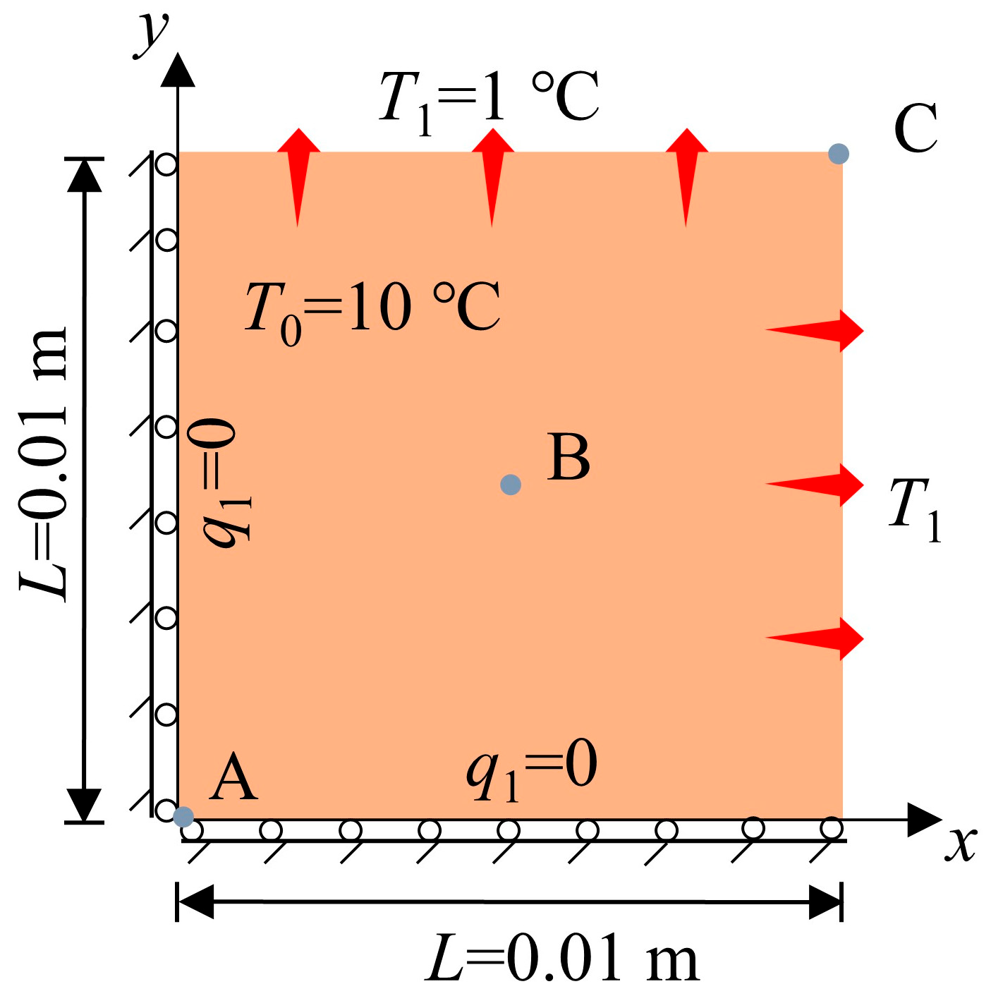
To validate the accuracy of the thermomechanical coupling model proposed in this study, the temperature and mechanical responses of a 2D square plate under a cooling load were simulated. Figure 3 shows the geometric model, initial conditions, and boundary conditions of the 2D square plate. The length of the 2D square plate is L = 0.01 m. The initial temperature is T₀ = 10 °C. The temperature boundary condition is T₁ = 1 °C. Adiabatic boundary conditions and normal displacement constraints were applied to the edges at x = 0 and y = 0.

For the PD simulation, the square plate was uniformly discretized with a material point spacing of Δx = 1.0 × 10⁻⁵ m, and the PD range radius was δ = 3Δx. The thermodynamic parameters of the material are as follows: elastic modulus E = 25.7 GPa, Poisson’s ratio v = 0.25, thermal conductivity k_T = 1.0 J/(s·m °C), density ρ = 1800 kg/m³, specific heat c_v = 1688 J/(kg·°C), and thermal expansion coefficient α = 1.8 × 10⁻⁵/°C.

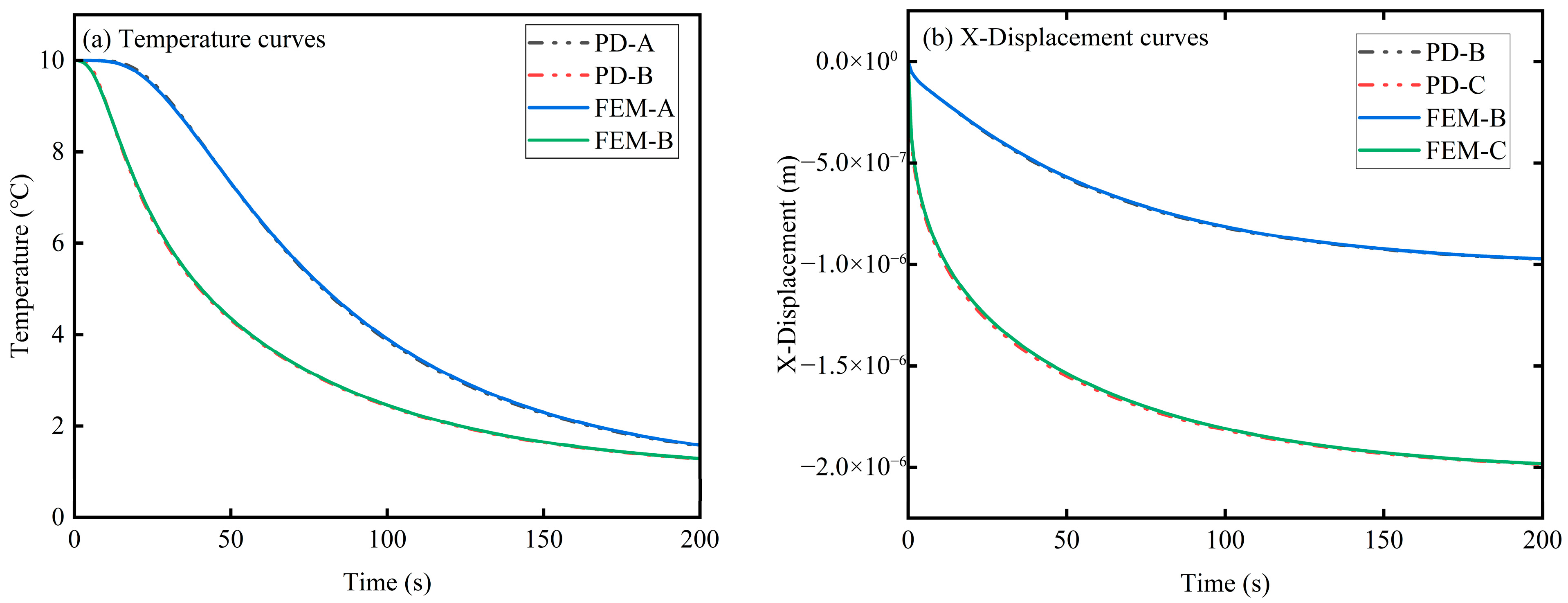
To quantitatively analyze the accuracy of the thermomechanical coupling model for temperature and displacement calculations, three observation points, A (0.0, 0.0), B (0.005, 0.005), and C (0.01, 0.01), are selected on the square plate. The temperature and horizontal displacement changes at these points, computed using the FEM and the PD method, are compared. As shown in Figure 4, the temperature curves at points A and B and the horizontal displacement curves at points B and C match well.

To further quantitatively analyze the computational accuracy, the global error ε is defined, and its expression is given by

$$\epsilon =\sqrt{{\displaystyle \frac{{\displaystyle \sum _{i=1}^{N_{\mathrm{total}}}{\left[y_i^{\left(\mathrm{r}\right)}-y_i^{\left(\mathrm{n}\right)}\right]}^2}}{{\displaystyle \sum _{i=1}^{N_{\mathrm{total}}}{\left[y_i^{\left(\mathrm{r}\right)}\right]}^2}}}}.$$

(12)

where N_total denotes the total number of data points. y^(r) is the reference solution, and y⁽ⁿ⁾ is the numerical solution. At point A, the error for temperature is 0.528%, while the error for horizontal displacement at point B is 0.551%. Similarly, the temperature error at point B is 0.682%, and the displacement error at point C is 0.631%. These results indicate that the thermomechanical coupling model based on the PD method provides highly accurate predictions, with global errors consistently low across different observation points. The relatively small discrepancies between the PD and FEM solutions highlight the effectiveness of the proposed model in simulating both temperature and mechanical response under cooling conditions.

The square plate is subjected to cooling loads on both sides, resulting in an overall decrease in temperature. Compared to point A, the faster cooling at point B can be attributed to its proximity to the cooling boundary, which results in more efficient heat dissipation. In contrast, the temperature at point A decreases more slowly due to the longer time required for heat to travel through the interior of the plate. As shown in Figure 4b, the horizontal displacement components at points B and C are negative, due to the normal displacement constraints applied to the left and bottom sides of the plate. After cooling, the plate exhibits an overall contraction toward the constrained regions.

Furthermore, to visually observe the changes in the temperature and displacement fields of the plate during the cooling process, Figure 5 presents the temperature and displacement distributions at four different time instances. As shown in Figure 5a, the cooling temperature boundary condition T₁ is applied to the top and right sides of the plate, whereas the remaining two sides were insulated. Therefore, cooling begins at the temperature boundary. As shown in Figure 5b, due to the combined effect of bidirectional cooling contraction and boundary constraints, the displacement at the top right corner of the plate is higher than elsewhere. Additionally, due to the symmetry of the 2D plate’s geometric structure, temperature boundary conditions, and displacement constraints with respect to y = x, both the temperature and displacement distributions in the plate are symmetric about y = x during the cooling process.

In summary, by comparing the results obtained using PD with those obtained using the FEM, it can be concluded that the proposed thermomechanical coupling model demonstrates good accuracy.

3.2. Quenching Simulation of a Ceramic Plate

The established PD thermomechanical coupling model was used to simulate the quenching process of an Al₂O₃ ceramic plate. The simulation results were compared with previous experimental data [35] to validate the accuracy of the model in predicting the thermomechanical damage and fracture behavior. In this experiment, the ceramic plate is first heated to 500 °C, and then is immersed in a water bath at 20 °C. The computational model is shown in Figure 6. The ceramic plate measures 50 mm × 10 mm, with an initial temperature of T₀ = 500 °C. Convective boundary conditions were applied on all four sides, and the ambient temperature was set to 20 °C.

In the PD simulation, the ceramic plate was uniformly discretized into 12,801 material points, each with a size of 2.0 × 10⁻⁴ m, and the horizon was set as δ = 3Δx. The thermomechanical properties of the ceramic plate are listed in

Table 1. Thermomechanical parameters of Al₂O₃ ceramic plates.

E	ν	ρ	GF	cv	kT	α
GPa		kg/m3	J/m2	J/(kg·°C)	J/(s·m·°C)	1/°C
370	1/3	3980	24.3	880	31	7.5 × 10−6

. The convective heat transfer coefficient between the solid and water was set to h = 70,000 W/(m²·°C). The time step was set to Δt = 5.0 × 10⁻⁶ s, and the total simulation time was 0.2 s.

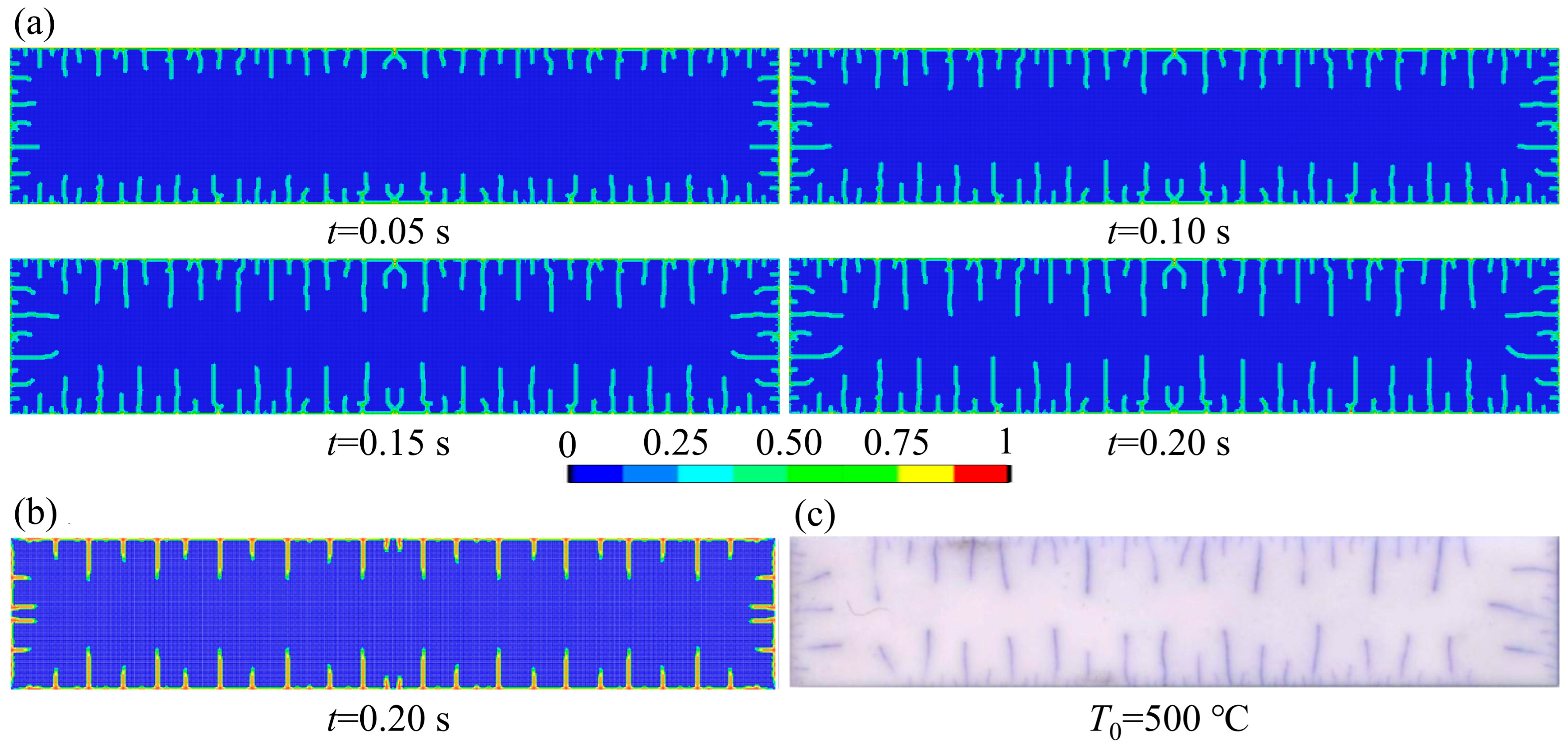
Figure 7a shows the evolution of the crack propagation path in the ceramic plate during the quenching process. The significant temperature difference between the initial temperature of the ceramic plate and the ambient temperature causes a sharp temperature drop at the edges of the plate during the initial stage of quenching, leading to a large temperature gradient. Due to the low thermal expansion coefficient and high brittleness of ceramics, significant thermal stresses develop both at the surface and inside the plate, inducing surface cracks.

The crack propagation path closely matches the simulation result in [36] and the experimental observation in [35], both initiating from the surface of the thin plate and extending inward, with the crack paths being nearly parallel.

4. Construction and Validation of the Deep Learning Model

As the complexity of thermodynamic problems increases, traditional computational methods face limitations, including high computational costs and complex solution processes, when handling dynamic loads and large-scale problems. To overcome these challenges, this section discusses the method of constructing a deep neural network (DNN) based on PD simulation data. By generating large amounts of simulation data through extensive computations and training a DL model on these data, a DNN is developed for fast prediction in thermomechanical coupling analysis.

4.1. Problem Description

The structural integrity of the RPV is a critical issue in the operation and life extension of nuclear power plants. In particular, verifying the RPV’s structural integrity under pressurized thermal shock conditions is crucial for ensuring the safe operation of the plant. In this context, the development of rapid analysis methods is essential for improving the efficiency of safety assessments, aiding in operational decision-making, and reducing the significant time and economic costs associated with more detailed analyses.

The plane strain model effectively simplifies the problem and significantly improves the computational efficiency. Taking the cylindrical section of a pressure vessel as an example, the model can be simplified as a 2D ring model. This section focuses on a 2D ring model, applying stable temperature boundary conditions, temperature boundary conditions with varying temperature, and pressure boundary conditions to analyze its thermomechanical coupling deformation behavior.

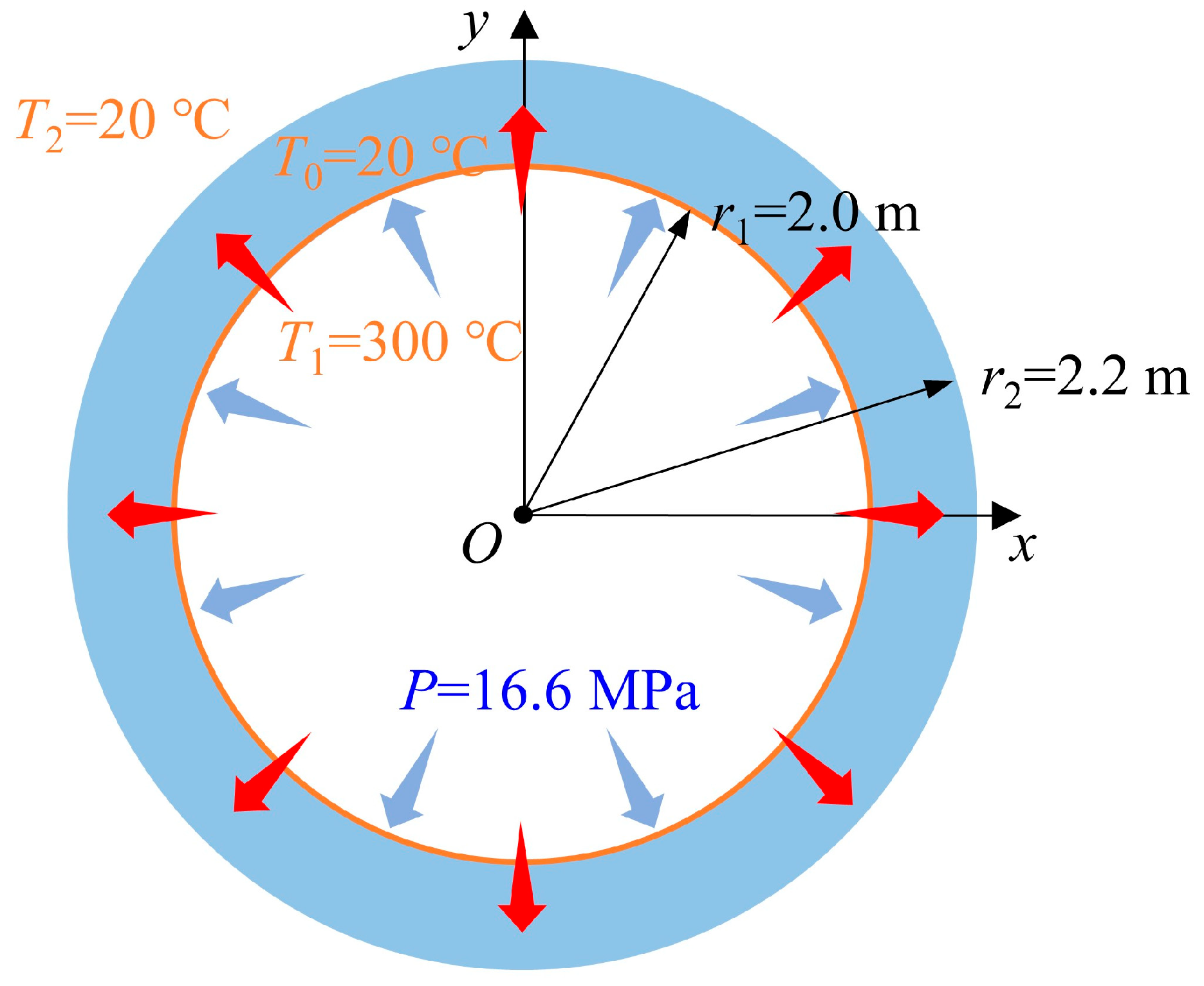
The geometric model of the 2D ring is shown in Figure 8, with an inner radius of 2.0 m and an outer radius of 2.2 m. In the PD model, the 2D ring was discretized into material points with the same radial length but varying widths. The material points were spaced radially at Δx = 6.25 × 10⁻³ m (with 32 layers of material points in the radial direction), and the PD range was δ = 3.015Δx. A temperature boundary condition of 320 °C was applied to the inner wall, and 20 °C was applied to the outer wall. The internal pressure was 16.6 MPa, with an initial temperature of 20 °C. A pressure boundary condition of 16.6 MPa was applied to the inner wall. The thermodynamic parameters of the 2D ring material are as follows: elastic modulus E = 191 GPa, Poisson’s ratio ν = 0.25, density ρ = 7769 kg/m³, specific heat c_v = 565.32 J/(kg·°C), thermal conductivity k_T = 39.246 J/(s·m·°C), and thermal expansion coefficient α = 1.34 × 10⁻⁵/°C.

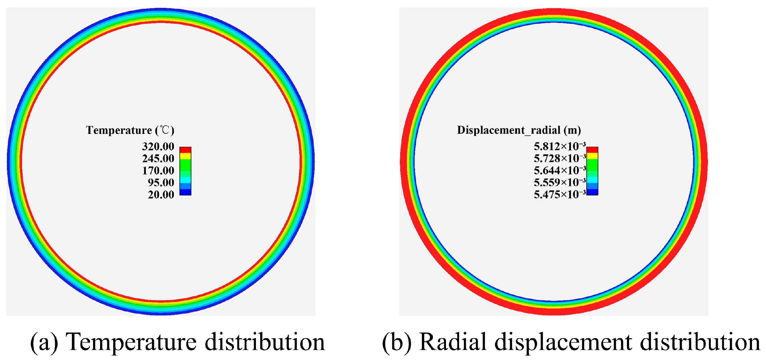
Figure 9 shows the temperature and radial displacement distributions of the 2D ring in the steady state. As shown in the figure, when the inner wall of the 2D ring is subjected to internal pressure and heating loads, both the temperature and radial displacement distributions exhibit a layered pattern. The temperature of the 2D ring decreases gradually from the inner wall to the outer wall, whereas the radial displacement increases from the inner wall to the outer wall. Under thermomechanical coupling loads, the inner wall experiences significant deformation due to thermal expansion and internal pressure. However, its proximity to the center and the strong geometric constraints cause the material points in the inner circle to be surrounded by more material, which greatly limits the deformation. The outer wall, being relatively “free”, responds more easily to the accumulated thermal expansion driving force from the interior. As heat is conducted from the inner wall to the outer wall, the entire structure undergoes gradient expansion. During this process, owing to material continuity, deformation in the inner layers is transferred to the outer layers; therefore, even when the inner layers experience higher stress, their displacement is overcome by the outer layers. Under the influence of the plane strain assumption and the symmetric geometric structure of the 2D ring, both the axial and circumferential displacements are zero, and the deformation of the 2D ring occurs along the radial direction.

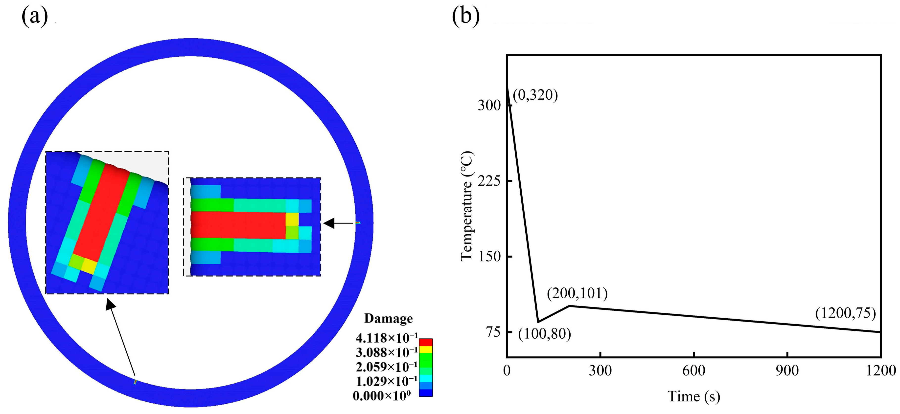
Under long-term thermomechanical loading, cracks can form on the surface of the cylindrical section of the pressure vessel. The initiation and propagation of these cracks affect the safety of the vessel. To simulate the deformation response of a pressure vessel under varying temperature loads after crack formation during service, two randomly generated cracks are introduced into the 2D ring geometry, as shown in Figure 10a, and the calculation formula for damage is given by Equation (6). The lengths of the two cracks are both 0.04375 m, with an angle of 141.25°. The temperature field distribution and deformation field distribution of the 2D ring in steady state from Figure 9 are selected, upon which varying temperature conditions [37] and an internal wall pressure of 16.6 MPa, as shown in Figure 10b, are applied.

After introducing cracks into the steady-state 2D ring shown in Figure 9, some bonds between the material points in the PD model break. Although the mechanical response of individual bonds remains unchanged, the disruption of local interactions reduces the number of effective bonds, disturbing the original equilibrium state. The introduction of cracks causes the structure to transition from a stable state to a non-equilibrium state. Therefore, before applying varying temperature conditions to the cracked 2D ring (at t = 0 s in Figure 10b), further calculations are performed to obtain the stable state of the cracked 2D ring.

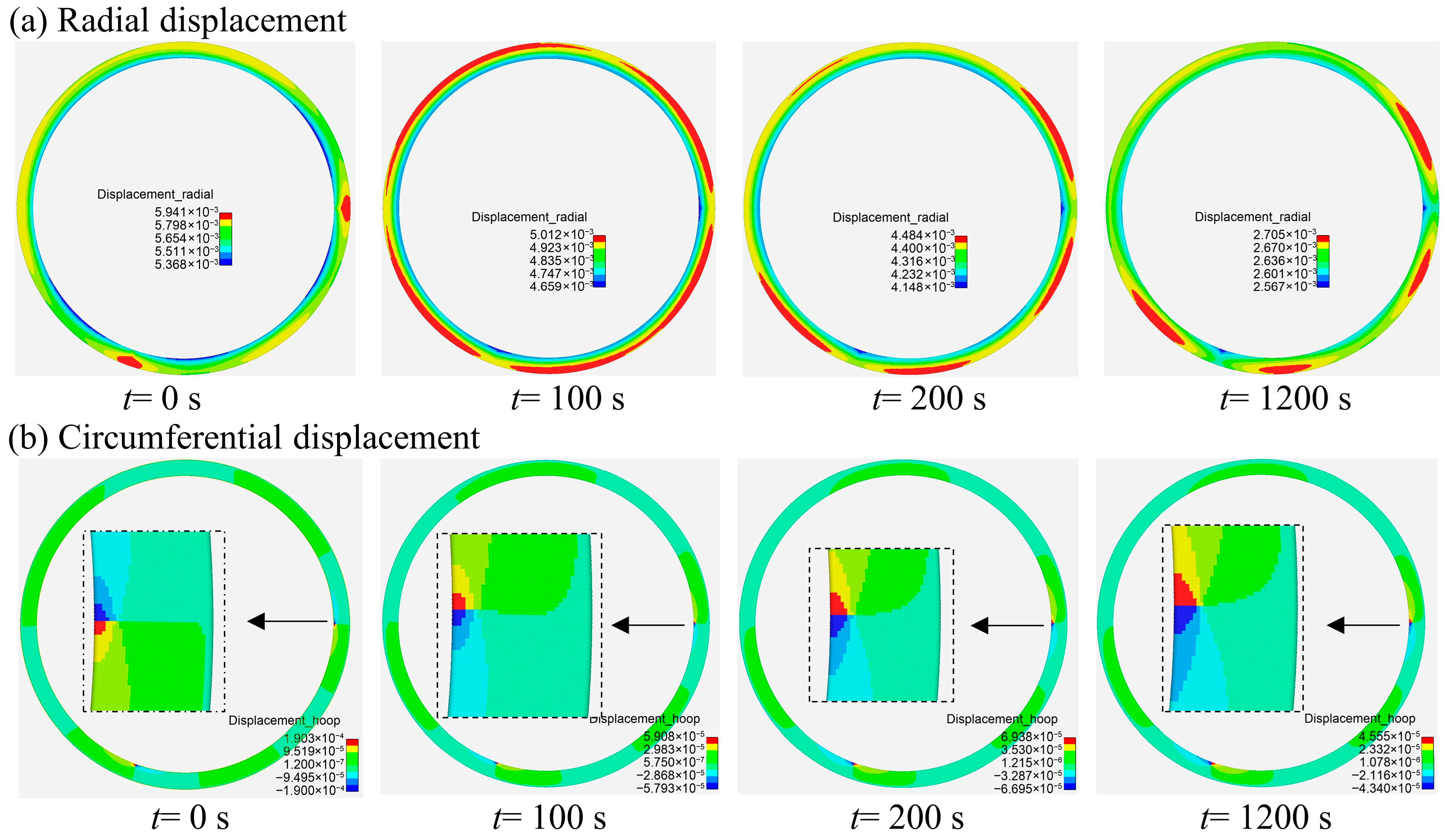
Figure 11a shows that the radial displacement of the ring gradually decreases over time. At the initial state (t = 0 s), the radial displacement is concentrated at the crack tips. However, as the varying temperature condition progresses, the displacement at the crack tips decreases, while larger radial displacements appear in the surrounding region. After the introduction of cracks, some material points near the cracks experience bond breakage, leading to a redistribution of circumferential stress and resulting in a noticeable circumferential displacement in the surrounding region. As shown in Figure 11b, the circumferential displacement distribution near the crack tip indicates that the inner wall transitions from a compressive to a tensile state. This is because during the cooling process, the inner wall experiences a rapid temperature drop and thermal contraction, resulting in tensile stress.

4.2. Large-Scale Computation

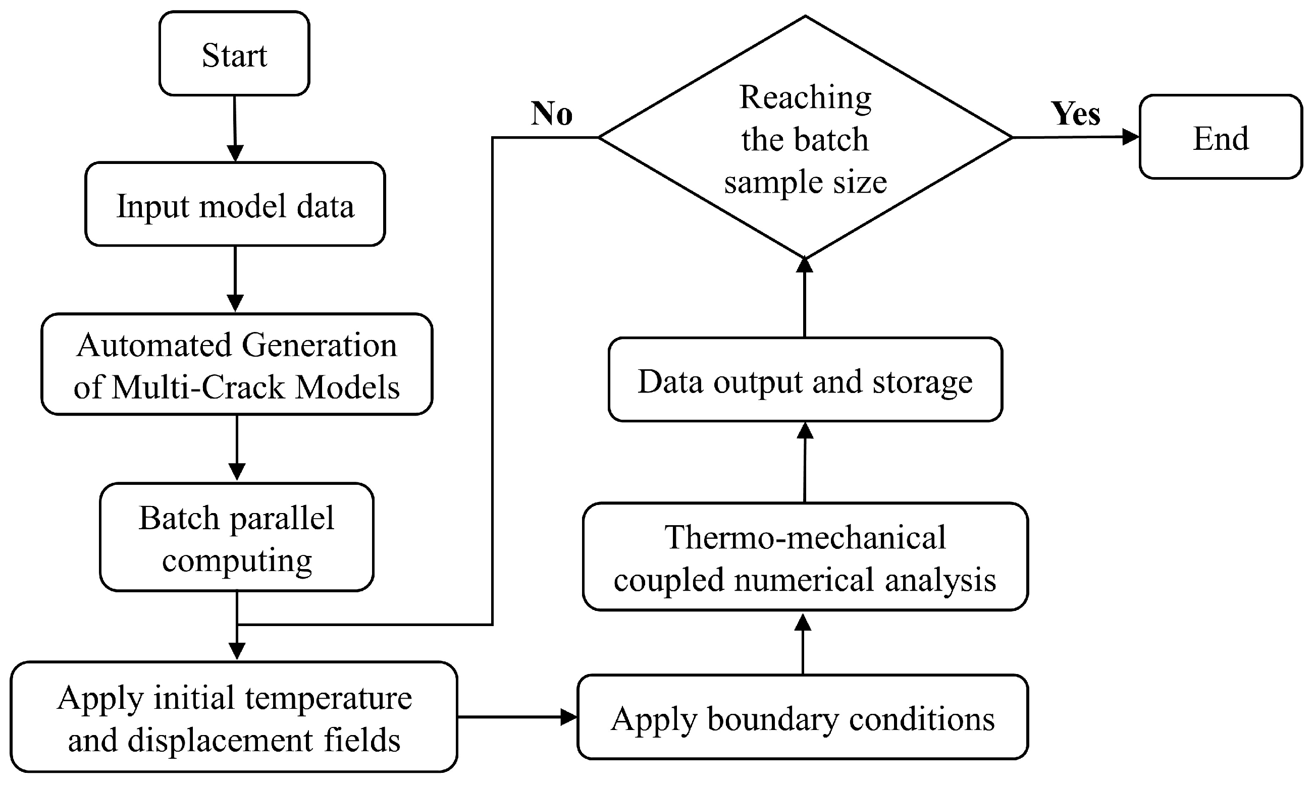
Large-scale numerical calculations were performed on a multiple-cracked 2D ring under varying temperature conditions to generate the necessary database for constructing a data-driven offline prediction model based on a DNN. To achieve this, a large-scale, high-throughput, concurrent numerical method was employed for damage and fracture analysis. Efficient parallel computing techniques were combined to simulate the deformation response of a multi-cracked 2D ring under varying temperature conditions. The high-throughput numerical analysis process is shown in Figure 12.

First, the temperature and deformation field distributions of the crack-free 2D ring in the steady state under the initial loading conditions were simulated, as shown in Figure 9. The number of material points, point IDs, temperature values, displacements, coordinates, damage index, bond force densities, and other properties of each bond in the steady-state 2D ring are stored as the initial conditions for subsequent calculations.

Next, to study the temperature and displacement distributions within the pressure vessel after a crack suddenly forms on the inner wall due to thermomechanical loading, a geometrical model of a multi-cracked 2D ring with different crack distributions was randomly generated for nearly 1000 sets using the code. Among them, there were two radial cracks in the ring; their lengths were less than or equal to one-quarter of the ring thickness (5 cm), with one crack fixed in position, ensuring that the angle between the two cracks was less than π. Nearly 1000 sets of geometrical models were divided into several groups and computed using different computational resources. At the start of the computation, the physical quantities of the steady-state 2D ring stored previously are used as the initial conditions. The temperature field, deformation field, and damage state distribution at the initial time (t = 0 s) under varying temperature conditions are then computed, without changing the steady-state temperature and pressure boundary conditions.

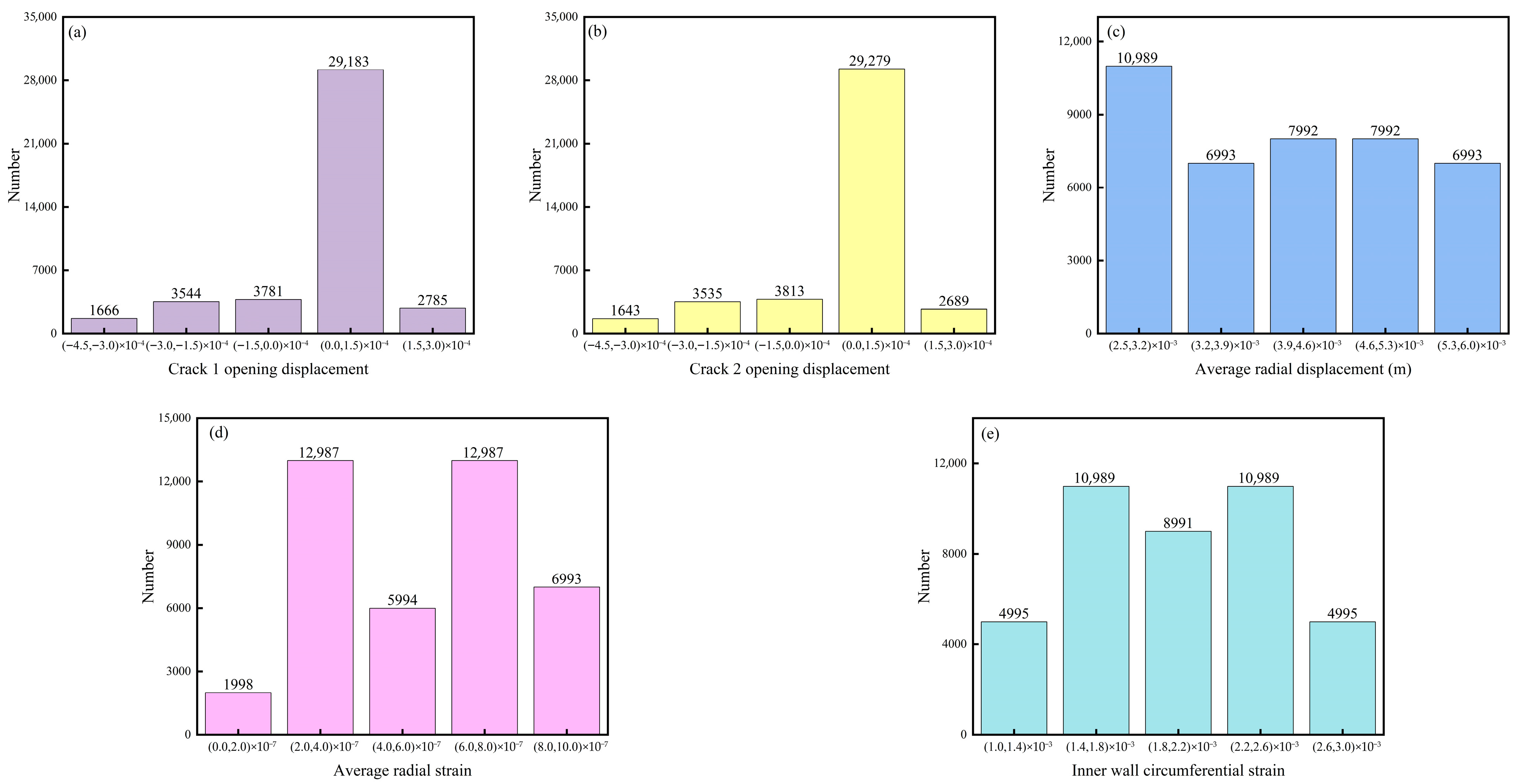
Finally, varying temperature boundary conditions, as shown in Figure 10b, are initially applied to the multi-cracked 2D ring under varying temperature conditions. The computations for nearly 1000 sets of multi-cracked 2D rings under varying temperature conditions result in a total of 40,959 datasets. The output variables include the inner wall temperature, inner wall pressure, crack 1 length, crack 2 length, angular difference between the cracks, crack tip opening displacement, average radial displacement, average radial strain, and inner wall circumference change rate of the 2D ring at different times under varying temperature conditions, providing reliable data for subsequent large-scale data analysis and model training. The crack tip opening displacement of the two cracks is calculated by the difference in the circumferential displacement between the material points at both ends of the radial crack on the inner wall of the 2D ring. The average radial displacement is the mean radial displacement of all material points in the 2D ring. The average radial strain is the mean radial strain at various locations on the ring. The rate of change in the inner wall circumference is calculated by dividing the change in the inner wall circumference after the deformation by the original inner wall circumference. The distribution of the output variables from the large-scale computations across different value ranges is shown in Figure 13.

4.3. Deep Learning Model Construction and Network Training

To approximate the nonlinear relationship between input parameters and mechanical responses under thermomechanical coupling, a DNN was constructed. The input for this problem is a six-dimensional vector consisting of the lengths of the first crack L₁, the second crack L₂, the angle between the two cracks θ, the inner wall temperature T, the time under varying temperature conditions t, and the inner wall pressure P. The outputs are the crack tip opening displacement D₁ for crack 1, the crack tip opening displacement D₂ for crack 2, the average radial displacement D_r of the 2D ring, the average radial strain D_s, and the change rate of the inner wall circumference C.

The DNN is trained using the large-scale PD simulation results presented in Section 4.2 as ground truth data, enabling it to serve as an efficient surrogate model for rapid mechanical response prediction. Considering the significant differences in the magnitude of the input and output variables, such as the fact that the average radial displacement and the average radial strain differ by up to four orders of magnitude, all input data are non-dimensionalized as shown in Equation (13) and all output data are normalized as shown in Equation (14).

$$\overline{x}={\displaystyle \frac{x}{\max \left(x\right)}},$$

(13)

$$\overline{y}={\displaystyle \frac{y-\min \left(y\right)}{\max \left(y\right)-\min \left(y\right)}}.$$

(14)

Here, $\overline{x}$ represents the non-dimensionalized data, $\overline{y}$ represents the normalized data, max(x) is the maximum value, and min(x) is the minimum value.

The network is trained by minimizing the mean squared error between predicted and true values, defined as

$$\mathrm{Loss}={\displaystyle \frac{1}{n}}{\displaystyle \sum _{i=1}^n{{\displaystyle \left({{\displaystyle y}}_i-{{\displaystyle \widehat{y}}}_i\right)}}^2},$$

(15)

where n is the number of samples, ${{\displaystyle \widehat{y}}}_i$ represents the predicted values from the neural network, y_i represents the true values, and ${{\displaystyle \overline{y}}}_i$ is the mean of the true values. To evaluate the predictive accuracy of the model, the coefficient of determination (R²) is employed:

$${{\displaystyle R}}^2=1-{\displaystyle \frac{{\displaystyle \sum _{i=1}^n{{\displaystyle \left({{\displaystyle y}}_i-{{\displaystyle \widehat{y}}}_i\right)}}^2}}{{\displaystyle \sum _{i=1}^n{{\displaystyle \left({{\displaystyle y}}_i-{{\displaystyle \overline{y}}}_i\right)}}^2}}}.$$

(16)

The model training cost is measured in terms of wall-clock time.

To determine an appropriate network structure, a series of comparative experiments are carried out by varying the number of neurons per hidden layer, while keeping the number of hidden layers fixed at two. As summarized in

Table 2. Average computational accuracy and training cost under different numbers of neurons per hidden layer.

Number of Neurons per Hidden Layer	Goodness of Fit	Training Cost (Minutes)
1	0.762	28.34
2	0.779	28.75
3	0.966	28.66
4	0.969	28.83
5	0.974	28.62
6	0.974	28.72
7	0.976	28.65
8	0.986	28.91
9	0.987	29.09
10	0.981	28.93
11	0.984	28.99
12	0.965	28.71
13	0.968	28.82
14	0.966	28.99
15	0.967	29.02

, the training time remains nearly constant (between 28 and 29 min), whereas the prediction accuracy initially increases and then declines as the number of neurons increases. The highest goodness of fit on the test set (R² = 0.987) is achieved when each hidden layer contained nine neurons. This indicates that insufficient neurons limit the model’s learning capacity, while excessive neurons introduce overfitting and impair generalization. Therefore, a neuron count of nine per layer is selected as the optimal choice.

Further experiments are conducted by fixing the number of neurons per layer at nine and varying the number of hidden layers. As shown in

Table 3. Average computational accuracy and training cost under different numbers of hidden layers.

Number of Hidden Layers	Goodness of Fit	Training Cost (Minutes)
1	0.934	27.29
2	0.987	29.09
3	0.985	30.85
4	0.969	34.72
5	0.956	37.88
6	0.876	47.22
7	0.886	49.85
8	0.872	52.98

, using two hidden layers achieves the best goodness-of-fit. This confirms that increasing the depth of the network beyond two layers does not lead to better generalization, but rather increases computational cost and potential overfitting. Thus, the final DNN architecture is determined to consist of two hidden layers, each containing nine neurons.

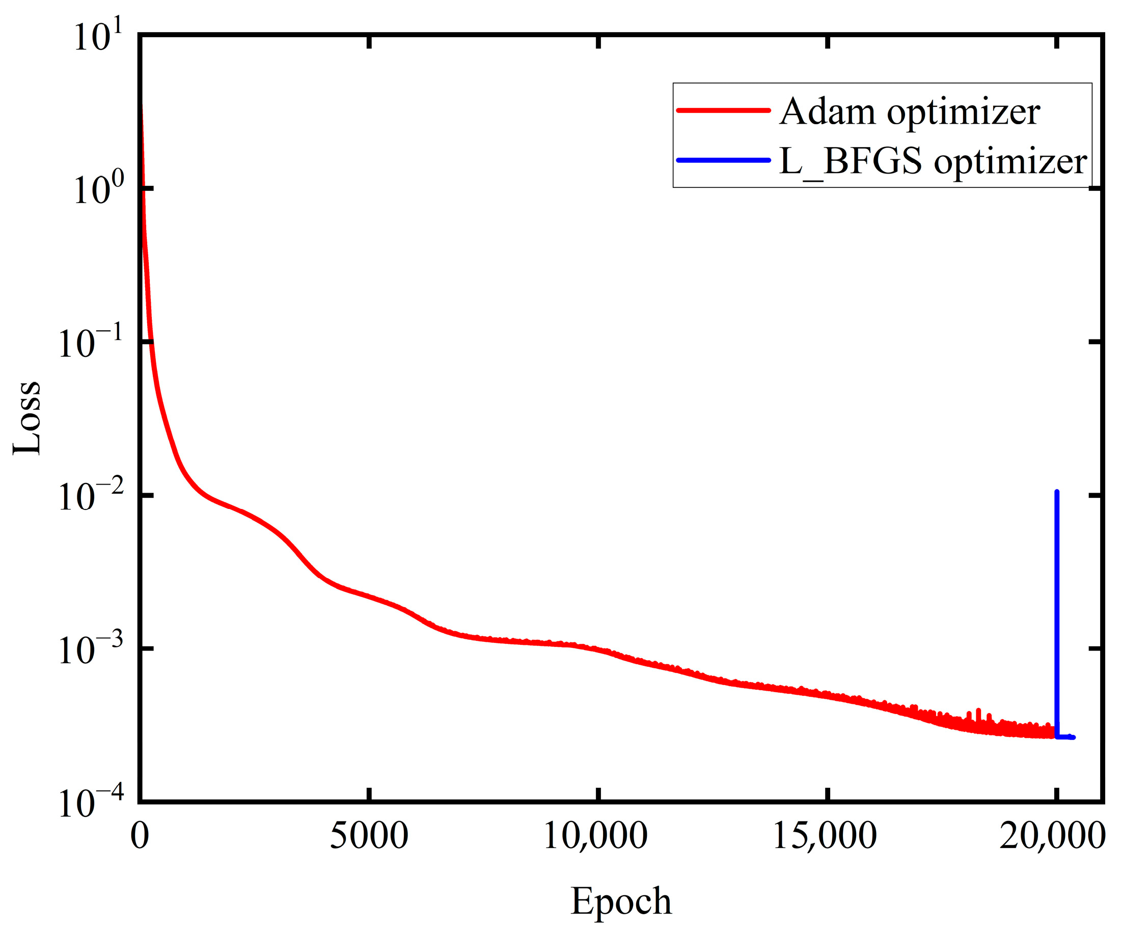
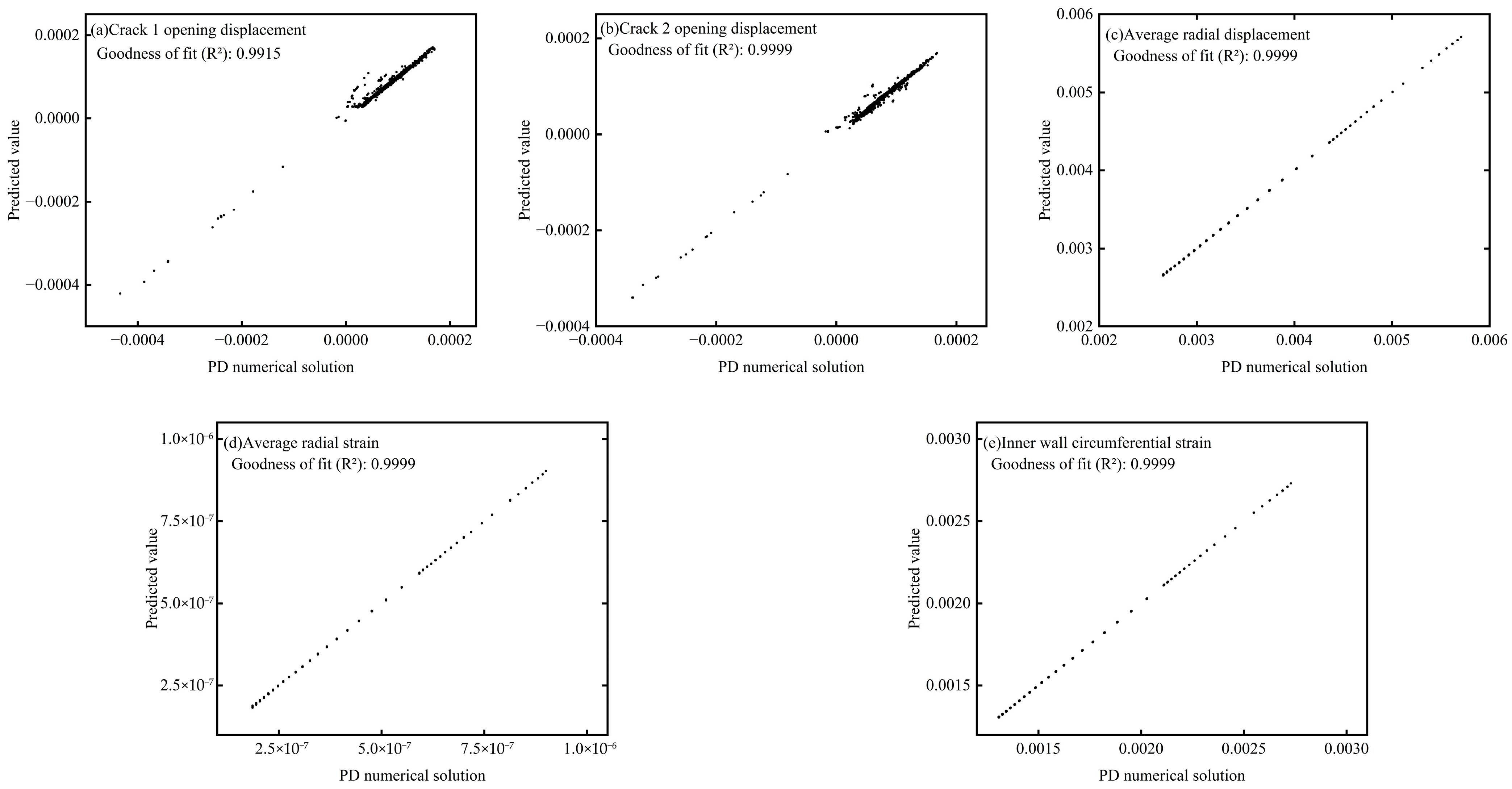
For the selected structure, the training process consists of two stages. Initially, the Adam optimizer is used for 20,000 iterations to achieve preliminary convergence. Subsequently, the L-BFGS optimizer is applied for an additional 300 iterations to further refine the model and reduce residual loss. The convergence behavior of the loss function is depicted in Figure 14. Finally, the trained model is evaluated on the test set. As shown in Figure 15, the predicted mechanical responses closely match the PD reference solutions, with most outputs achieving R² > 0.99, confirming that the trained DNN exhibits excellent accuracy and generalization capability for multi-output mechanical prediction tasks.

4.4. Thermomechanical Coupling Deformation Behavior Prediction

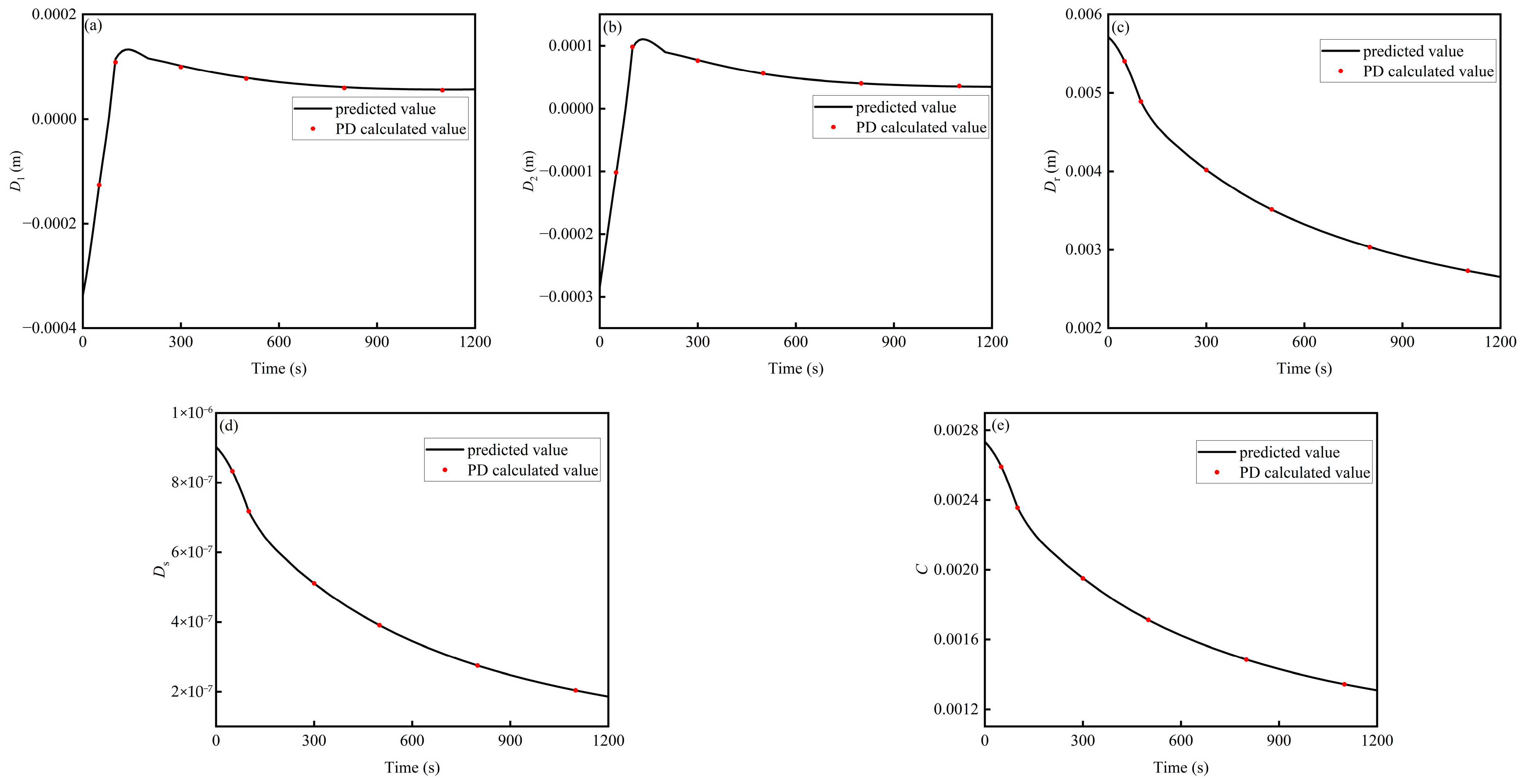
Two cracks are randomly generated in a two-dimensional circular ring, with the first crack having a length of L₁ = 0.0375 m and the second crack having a length of L₂ = 0.03125 m. The angle between the two cracks is θ = 119.41°. The crack distribution, along with the temperature conditions under varying temperatures (as shown in Figure 10b), including the corresponding time, temperature, and pressure, are input into the network trained in Section 4.3. The network is capable of predicting the opening displacements of the two cracks (D₁ and D₂), the average radial displacement D_r of the two-dimensional ring, the average radial strain D_s, and the change rate of the inner wall circumference C at different time instances. To further validate the efficiency and accuracy of the neural network predictions, the deformation characteristics of the two-dimensional ring during the temperature variation process under the given crack distribution are calculated using PD.

Figure 16a–e present the results of five output variables at different times, obtained from both the neural network predictions and the PD calculations. The results show good agreement between the two methods. However, it is noteworthy that the neural network prediction takes only approximately 0.5 s, while the PD calculation requires approximately 10 min. This demonstrates that the neural-network-based prediction method achieves a computational efficiency improvement of approximately 1200 times, highlighting its significant advantage in handling similar problems.

5. Conclusions

This study introduces an innovative approach for modeling thermomechanical failure in critical structures under extreme conditions by combining peridynamics (PD) with deep learning (DL). The proposed PD thermomechanical coupling model, utilizing the BBPD for structural deformation and the peridynamic differential operator for thermal diffusion, successfully captures the nonlocal interactions associated with crack propagation and thermal stresses. Through comprehensive validation, including simulations of a 2D plate under cooling and the quenching process of an Al₂O₃ ceramic, the model demonstrates excellent accuracy compared to the conventional FEM and experimental data. Furthermore, the integration of DL, specifically a deep neural network, trained on large datasets generated by PD simulations, offers a significant enhancement in computational efficiency, achieving prediction speeds approximately 1200 times faster than those of direct PD simulations without compromising accuracy.

The PD-DL framework provides a promising direction for real-time analysis and fault prediction in thermomechanical coupling problems, particularly in engineering applications involving critical structures, such as pressure vessels. Future research could focus on extending the framework to complex materials, like composites, and improving the DL surrogate model to handle larger datasets and enhance generalization. Additionally, integrating this framework with structural health monitoring systems could offer a comprehensive solution for real-time damage detection and predictive maintenance in critical infrastructure.

References

1. Li, Y.; Jin, T.; Wang, Z.; Wang, D. Engineering critical assessment of RPV with nozzle corner cracks under pressurized thermal shocks. Nucl. Eng. Technol. 2020, 52, 2638–2651. [Google Scholar] [CrossRef]
2. Liu, Z.; Li, Z.; Ma, Q. A thermo-mechanical coupling model for simulating the re-entry failure evolution mechanism of spacecraft propulsion module. Thin-Walled Struct. 2023, 184, 110504. [Google Scholar] [CrossRef]
3. Chen, W.; Dai, S.; Zheng, B. Continuum damage dynamic model combined with transient elastic equation and heat conduction equation to solve RPV stress. Fractal Fract 2022, 6, 215. [Google Scholar] [CrossRef]
4. Annor-Nyarko, M.; Xia, H. Numerical fracture analysis of a reactor pressure vessel based on Abaqus-FRANC3D co-simulation method. Procedia Struct. Integr. 2022, 37, 225–232. [Google Scholar] [CrossRef]
5. Han, D.; Fan, H.; Yan, C.; Wang, T.; Yang, Y.; Ali, S.; Wang, G. Heat conduction and cracking of functionally graded materials using an FDEM-Based thermo-mechanical coupling model. Appl. Sci. 2022, 12, 12279. [Google Scholar] [CrossRef]
6. An, X.; Fu, G.; Ma, G. A comparison between the NMM and the XFEM in discontinuity modeling. Int. J. Comput. Methods 2012, 9, 1240030. [Google Scholar] [CrossRef]
7. Lin, Y.W.; Chang, K.H.; Chen, C.K. Hybrid differential transform method/smoothed particle hydrodynamics and DT/finite difference method for transient heat conduction problems. Int. Commun. Heat Mass Transf. 2020, 113, 104495. [Google Scholar] [CrossRef]
8. Yu, S.; Ren, X.; Zhang, J. Using an improved SPH algorithm to simulate thermo-hydro-mechanical-damage coupling problems in rock masses. Case Stud. Therm. Eng. 2023, 47, 103085. [Google Scholar] [CrossRef]
9. Zhang, L.; Zheng, H. MLS-based numerical manifold method based on IPIM for 3D transient heat conduction of FGMs. Int. J. Heat Mass Transf. 2023, 217, 124704. [Google Scholar] [CrossRef]
10. Zhang, L.; Zheng, H.; Liu, F. MLS-based numerical manifold method for steady-state three-dimensional heat conduction problems of functionally graded materials. Comput. Math. Appl. 2023, 144, 124–140. [Google Scholar] [CrossRef]
11. Li, D.; Li, P.; Li, W.; Li, W.; Zhou, K. Three-dimensional phase-field modeling of temperature-dependent thermal shock-induced fracture in ceramic materials. Eng. Fract. Mech. 2022, 268, 108444. [Google Scholar] [CrossRef]
12. Shen, Z.; Wang, J.; Jiang, J.; Huang, S.X.; Lin, Y.; Nan, C.; Chen, L.; Shen, Y. Phase-field modeling and machine learning of electric-thermal-mechanical breakdown of polymer-based dielectrics. Nat Commun 2019, 10, 1843. [Google Scholar] [CrossRef]
13. Xin, Y.; Li, Z.; Huang, D.; Lu, Y. An electromechanical coupling peridynamic model for piezoelectric solids with defects. Int. J. Mech. Sci. 2025, 304, 110679. [Google Scholar] [CrossRef]
14. Silling, S.A.; Askari, E. A meshfree method based on the peridynamic model of solid mechanics. Comput. Struct. 2005, 83, 1526–1535. [Google Scholar] [CrossRef]
15. Silling, S.A. Reformulation of elasticity theory for discontinuities and long-range forces. J. Mech. Phys. Solids 2000, 48, 175–209. [Google Scholar] [CrossRef]
16. Wang, Y.; Zhou, X.; Kou, M. Peridynamic investigation on thermal fracturing behavior of ceramic nuclear fuel pellets under power cycles. Ceram. Int. 2018, 44, 11512–11542. [Google Scholar] [CrossRef]
17. Zhang, H.; Huang, D. A peridynamic thermal contact model for heat conduction analysis of thermally imperfect interface and conductive crack. Int. J. Heat Mass Transf. 2025, 241, 126763. [Google Scholar] [CrossRef]
18. Gu, X.; Zhang, Q.; Madenci, E.; Xia, X. Possible causes of numerical oscillations in non-ordinary state-based peridynamics and a bond-associated higher-order stabilized model. Comput. Methods Appl. Mech. Eng. 2019, 357, 112592. [Google Scholar] [CrossRef]
19. Oterkus, S.; Madenci, E.; Agwai, A. Fully coupled peridynamic thermomechanics. J. Mech. Phys. Solids 2014, 64, 1–23. [Google Scholar] [CrossRef]
20. Wang, Y.; Zhou, X.; Kou, M. A coupled thermo-mechanical bond-based peridynamics for simulating thermal cracking in rocks. Int. J. Fract. 2018, 211, 13–42. [Google Scholar] [CrossRef]
21. Wang, Y.; Zhou, X.; Kou, M. An improved coupled thermo-mechanic bond-based peridynamic model for cracking behaviors in brittle solids subjected to thermal shocks. Eur. J. Mech. A/Solids 2019, 73, 282–305. [Google Scholar] [CrossRef]
22. He, D.; Huang, D.; Wu, L.; Xu, Y. Investigation on thermal failure of functionally graded materials using fully coupled thermo-mechanical peridynamics. Compos. Struct. 2023, 305, 116454. [Google Scholar] [CrossRef]
23. Yang, C.; Zhu, F.; Zhao, J. A multi-horizon fully coupled thermo-mechanical peridynamics. J. Mech. Phys. Solids 2024, 191, 105758. [Google Scholar] [CrossRef]
24. Wang, X.; Dong, W.; He, Q.; An, B.; Ding, H.; Wang, P.; Wang, W.; Huang, J. Nonlocal thermomechanical coupled analysis of wheel-rail contact using a peridynamic model. Wear 2023, 528–529, 204954. [Google Scholar] [CrossRef]
25. Liu, S.; Han, F.; Deng, X.; Lin, Y. Thermomechanical peridynamic modeling for ductile fracture. Materials 2023, 16, 4074. [Google Scholar] [CrossRef]
26. Zhang, J.; Guo, L. A fully coupled thermo-mechanical peridynamic model for cracking analysis of frozen rocks. Comput. Geotech. 2023, 164, 105809. [Google Scholar] [CrossRef]
27. Murtaza, U.T.; Javed Hyder, M. The effects of thermal stresses on the elliptical surface cracks in PWR reactor pressure vessel. Theor. Appl. Fract. Mech. 2015, 75, 124–136. [Google Scholar] [CrossRef]
28. Choi, Y.; Cho, N.; Yang, J.; Yun, H.; Lee, H.; Huh, N. Shakedown and limit analyses of a pressurised water reactor vessel nozzle under cyclic thermo-mechanical loadings. Nucl. Eng. Des. 2022, 397, 111947. [Google Scholar] [CrossRef]
29. Zhuang, W.; Wang, E.; Zhang, H. Prediction of compressive mechanical properties of three-dimensional mesoscopic aluminium foam based on deep learning method. Mech. Mater. 2023, 182, 104684. [Google Scholar] [CrossRef]
30. Yang, J.; Kang, G.; Kan, Q. A novel deep learning approach of multiaxial fatigue life-prediction with a self-attention mechanism characterizing the effects of loading history and varying temperature. Int. J. Fatigue 2022, 162, 106851. [Google Scholar] [CrossRef]
31. Tang, M.; Wang, L.; Xin, Z.; Luo, Z. High energy absorption design of porous metals using deep learning. Int. J. Mech. Sci. 2024, 282, 109593. [Google Scholar] [CrossRef]
32. Madenci, E.; Barut, A.; Futch, M. Peridynamic differential operator and its applications. Comput. Methods Appl. Mech. Eng. 2016, 304, 408–451. [Google Scholar] [CrossRef]
33. Zhang, Z.; Wang, L.; Gu, X.; Li, H.; Zhang, Y.; Wu, Y. Fundamental solution-embedded peridynamic differential operator modeling for thermal conduction. Int. J. Mech. Sci. 2025, 287, 109991. [Google Scholar] [CrossRef]
34. Hahn, D.W.; Özisik, M.N. Heat Conduction; John Wiley & Sons: Chichester, UK, 2012. [Google Scholar]
35. Li, J.; Song, F.; Jiang, C. Direct numerical simulations on crack formation in ceramic materials under thermal shock by using a non-local fracture model. J. Eur. Ceram. Soc. 2013, 33, 2677–2687. [Google Scholar] [CrossRef]
36. Li, H.; Zhang, H.; Zhang, Y.; Bai, X.; Shao, X.; Wu, B. Coupled non-ordinary state-based peridynamics model for ductile and brittle solids subjected to thermal shocks. Appl. Sci. 2024, 14, 6927. [Google Scholar] [CrossRef]
37. Zhu, D.; Sun, H.; Zheng, B.; Huang, T.; Deng, J.; Xu, Y.; Luo, Y. Study on thermal shock failure characteristics of RPV during IVR system start-up for typical advanced PWR. Front. Energy Res. 2022, 10, 899405. [Google Scholar] [CrossRef]
Figure 1. Interactions between material points.
Applsci 15 10032 g001
Figure 2. Sequential coupling computation flowchart.
Applsci 15 10032 g002
Figure 3. A two-dimensional plate subjected to a cooling load. The square plate has a side length of L = 0.1 m. Two sides are subject to temperature boundary conditions of T1 = 1 °C, while the remaining two sides are insulated with adiabatic boundary conditions. The initial temperature is T0 = 10 °C. The red arrows indicate the direction of heat flow. Points A, B, and C are observation points with coordinates (0.0, 0.0), (0.005, 0.005), and (0.01, 0.01), respectively.
Applsci 15 10032 g003
Figure 4. Temperature and displacement curves obtained by PD and FEM simulations. The (a) temperature–time curves and (b) displacement–time curves. The temperature–time and displacement–time curves at different positions of the square plate obtained by the two methods are in good agreement.
Applsci 15 10032 g004
Figure 5. Temperature and displacement distribution of a square plate during the cooling process. The (a) temperature distribution and (b) displacement distribution. Based on the symmetry of geometric structure, temperature boundary and displacement constraints, the temperature and displacement distributions are symmetric with respect to y = x.
Applsci 15 10032 g005
Figure 6. Geometric model and corresponding boundary conditions for simulating the quenching process of the Al2O3 ceramic plate. The initial temperature of the ceramic plate was set to 500 °C, and the ambient temperature was maintained at 20 °C. The red arrows indicate the direction of heat flow.
Applsci 15 10032 g006
Figure 7. Comparison of damage distributions during the quenching of the ceramic plate: (a) damage results of BBPD, (b) damage result of SBPD [36], and (c) experimental observation [35].
Applsci 15 10032 g007
Figure 8. Geometry of the 2D ring. The inner radius r1 is 2.0 m and the outer radius r2 is 2.2 m. Temperature boundary conditions of 320 °C and 20 °C were applied to the inner and outer walls, respectively. The red arrows indicate the direction of heat flow. A pressure of 16.6 MPa was applied to the inner wall. The blue arrows indicate the direction of pressure.
Applsci 15 10032 g008
Figure 9. Distribution of temperature field and radial displacement in the 2D ring at steady state. (a) Temperature distribution; (b) Displacement distribution. Both temperature and displacement exhibit a layered distribution.
Applsci 15 10032 g009
Figure 10. Geometric configuration of a 2D ring with cracks and time-varying temperature boundary conditions applied to the inner wall [37]. (a) 2D ring with cracks; (b) variable temperature boundary condition. The two cracks are each 0.04375 m in length with an included angle of 141.25°.
Applsci 15 10032 g010
Figure 11. Displacement distributions of the 2D ring with multiple cracks under time-varying temperature conditions. (a) Radial displacement distribution, and (b) circumferential displacement distribution.
Applsci 15 10032 g011
Figure 12. Large-scale computing workflow.
Applsci 15 10032 g012
Figure 13. Distribution of large-scale simulation data for a 2D ring with cracks. (a) crack 1 opening displacement distribution; (b) crack 2 opening displacement distribution; (c) average radial displacement distribution; (d) average radial strain distribution; (e) inner wall circumferential strain distribution.
Applsci 15 10032 g013
Figure 14. Convergence of the loss function with two optimizers.
Applsci 15 10032 g014
Figure 15. Comparison between DNN predicted values and PD numerical solutions under time-varying temperature conditions: (a) crack 1 opening displacement, (b) crack 2 opening displacement, (c) average radial displacement, (d) average radial strain, and (e) inner wall circumferential strain.
Applsci 15 10032 g015
Figure 16. Deformation characteristics change with temperature change conditions. (a) crack 1 opening displacement. (b) crack 2 opening displacement. (c) average radial displacement. (d) average radial strain. (e) inner wall circumferential strain.
Applsci 15 10032 g016