Three-Dimensional Time-Lapse Joint Inversion of Resistivity and Time-Domain Induced Polarization Methods

Abstract

The resistivity method and time-domain induced polarization (TDIP) method are two branches of electrical geophysical prospecting. In recent years, researchers have implemented time-lapse resistivity inversion and time-lapse TDIP inversion based on time-lapse constraint theory. Although time-lapse inversion ensures temporal continuity between inversion results obtained at distinct epochs, it may not only cause the results to deviate from the true subsurface conditions, but also result in significant structural discrepancies resistivity and TDIP inversion results, thereby reducing inversion accuracy. To address these issues, the joint inversion of time-lapse resistivity and TDIP data was implemented based on cross-gradient constraint theory and time-lapse constraint theory. Using synthetic data from the theoretical model, we conducted separate inversion, time-lapse inversion, and time-lapse joint inversion. Comparative analysis of the results from these inversion schemes reveals that, compared with separate inversion and time-lapse inversion, time-lapse joint inversion not only maintains the temporal continuity of inverted models across consecutive monitoring epochs but also enforces structural similarity among distinct physical property models. This approach significantly increases the accuracy of the inversion results and exhibits superior noise robustness. These findings confirm the stability, reliability, and superiority of the algorithm developed in this study, providing a novel approach for addressing geological monitoring challenges.

1. Introduction

Time-lapse inversion results in the acquisition of differential data through repeated observations of a target area at distinct epochs, enabling monitoring of subsurface geological changes. The multielectrode and multichannel systems used in the resistivity and TDIP methods facilitate efficient large-scale data acquisition, positioning these techniques as pivotal domains for the advancement of time-lapse inversion.

Early work by Daily [1] demonstrated the potential of resistivity methods to monitor groundwater infiltration processes through repeated measurements. However, this approach resulted in the acquisition of data at discrete epochs without incorporating temporal correlations between datasets. Subsequent research established that normalizing observational datasets prior to inversion—filtering spurious anomalies associated with initial models—enhances the detection of subtle variations in subsurface properties when fed into conventional inversion algorithms [2]. By building normalization frameworks, researchers have incorporated background data inversion results as prior models for time-lapse inversions, resulting in accelerated convergence and reduced data misfit [3]. In previous methodologies, the temporal continuity of subsurface property changes was neglected, hindering accurate representations of evolutionary trends. Kim [4] pioneered a new method for time-lapse resistivity inversion, in which a temporal constraint function enables simultaneous inversion of multi-epoch datasets through mutual cross-epoch regularization; this ensures continuous temporal variation in the inversion results. Hayley [5] confirmed the superiority of this simultaneous approach through comparative analysis with alternative time-lapse methods. Subsequent research has advanced both time-lapse resistivity and TDIP methodologies: Kim achieved prior model-constrained 2D resistivity time-lapse inversion [6]; Karaoulis [7] developed specialized software for 4D resistivity-IP time-lapse inversion; and Zhu [8] realized 3D resistivity time-lapse inversion via the limited-memory BFGS optimization method.

Despite considerable maturity in principles and applications, persistent challenges remain. The first challenge is that time-lapse inversion’s emphasis on temporal continuity often compromises per-epoch accuracy, as the temporal constraint enhances cross-epoch coherence at the expense of the precision of individual results; the second challenge is that significant structural discrepancies arise between resistivity and polarizability models owing to complex subsurface property distributions, generating divergent spatial patterns and structural features that obstruct mutually consistent interpretation.

Geophysical joint inversion integrates complementary physical properties to characterize subsurface targets from multidimensional perspectives, yielding interpretations that more closely approximate geological reality. Gallardo and Meju pioneered this approach through cross-gradient structural constraints, progressively implementing two-dimensional joint inversion of seismic travel-time and DC resistivity data; magnetotelluric and seismic travel-time joint inversion; and multi-property joint inversion unifying marine seismic reflection, marine MT, gravity, and magnetic field measurements [9,10,11,12]. Zhu [13] extended this framework by establishing three-dimensional joint inversion for resistivity and TDIP methods via cross-gradient structural constraints.

In this study, we conduct research on 3D time-lapse joint inversion of resistivity and TDIP methods. By combining the strengths of both time-lapse inversion and joint inversion, we aim to ensure the temporal continuity of inversion results across distinct epochs while mutually constraining the resistivity and polarizability models. This integrated approach overcomes the limitations of separate-method inversions, reduces solution non-uniqueness, enhances inversion accuracy, and has significant scientific merit and application potential.

2. Rationale and Theory

2.1. Forward Modeling Algorithm

In this study, we utilize the finite-difference method to perform three-dimensional forward modeling of resistivity surveys. Building on the forward modeling theory established by Zhu [13] for resistivity methods, the governing partial differential equation for point-source resistivity is expressed as:

$$\mathit{\nabla }\left[\sigma \left(x,y,z\right)\mathit{\nabla }\phi \left(x,y,z\right)\right]=-j\delta (x-x_0)\delta (y-y_0)\delta (z-z_0),$$

(1)

where $\sigma$ represents the electrical conductivity of the rock ore (S·m⁻¹), $\phi$ denotes the potential array (V), $j$ is the power supply current intensity (A·m⁻²), and $\delta$ is a Dirac function, which specifies the position of the supply point.

The finite-difference method was applied to discretize (1), yielding a large sparse linear system of equations expressed in matrix form as:

$$A\phi =b,$$

(2)

where $A$ represents the coefficient matrix, and where $b$ denotes the source term vector containing field source information.

In this study, we solve the electric potential system via the biconjugate gradient stabilized (BICGSTAB) method with ILU preconditioning [14]. The apparent resistivity ${\rho }_a$ is then calculated from the potential field via (3).

$$\left\{\begin{array}{l}U=\alpha \phi \\ {\rho }_a=K{\displaystyle \frac{\Delta U}{I}}\end{array}\right.,$$

(3)

where $\alpha$ is a vector that is designed to select the potential at the receiver among all grid node potentials; $\Delta U$ is the potential difference between the receiving electrodes; and $K$ is the geometric factor.

The distinction between TDIP and resistivity forward modeling is determined by whether polarization phenomena are accounted for. Consequently, the total electric field in IP numerical simulations comprises two components: the primary field unaffected by IP effects and the secondary polarization field generated by IP effects.

The total field calculation involves a two-step procedure: first, the background potential (or potential difference) without polarization effects is computed via forward modeling; second, the conductivity $\sigma$ in (1) is substituted with the polarization-modified conductivity ${\sigma }_{\eta }$ from (4); then, the polarization-incorporated potential $u_{\eta }$ is derived through forward modeling. The apparent polarizability ${\eta }_a$ is subsequently calculated using (5) [15].

$${\sigma }_{\eta }=\sigma (1-\eta ),$$

(4)

where $\eta$ is the polarizability of the anomaly, which is dimensionless.

$${\eta }_a={\displaystyle \frac{u_{\eta }-u}{u_{\eta }}}.$$

(5)

2.2. Time-Lapse Joint Inversion Algorithm

2.2.1. Time-Lapse Constraint

To ensure temporal coherence in inversion results across different epochs, a time-lapse constraint function is introduced. This constraint promotes smooth transitions between models at successive time steps. In a typical time-lapse inversion framework, data from multiple epochs are inverted simultaneously while incorporating this temporal regularization. In our joint inversion scheme, we adopt a similar strategy; however, the inversion parameters are extended from single resistivity to include both resistivity and polarizability. The conductivity model at epoch $\mathit{i}$ is denoted as ${\mathit{m}}_{\mathit{\sigma },\mathit{i}}$, and the polarizability model as ${\mathit{m}}_{\mathit{\eta },\mathit{i}}$. The combined time-lapse model vectors are represented as ${\mathit{M}}_{\mathit{\sigma }}$ and ${\mathit{M}}_{\mathit{\eta }}$, respectively.

$$\left\{\begin{array}{l}{\mathit{M}}_{\mathit{\sigma }}={\left[{\mathit{m}}_{\mathit{\sigma },\mathbf{1}}{\mathit{m}}_{\mathit{\sigma },\mathbf{2}}\dots {\mathit{m}}_{\mathit{\sigma },\mathit{n}\mathit{t}}\right]}^T\\ {\mathit{M}}_{\mathit{\eta }}={\left[{\mathit{m}}_{\mathit{\eta },\mathbf{1}}{\mathit{m}}_{\mathit{\eta },\mathbf{2}}\dots {\mathit{m}}_{\mathit{\eta },\mathit{n}\mathit{t}}\right]}^T\end{array}\right.,$$

(6)

where $\mathit{n}\mathit{t}$ is the number of epochs.

In conventional inversion, the objective function typically adopts either the L1-norm or the L2-norm formulation, and this also holds true for time-lapse inversion frameworks [16,17]. The L2-norm encourages stronger temporal continuity between inversion results, enabling a more integrated interpretation of subsurface changes over time. In contrast, the L1-norm tends to preserve sharp localized variations across epochs by minimizing excessive temporal smoothing [6]. Considering the widespread adoption of the L2-norm and the convergence challenges often encountered with L1-based approaches in field data applications, we implement the L2-norm formulation in our framework. This is expressed mathematically as:

$$\left\{\begin{array}{l}{\Phi }_t\left({\mathit{M}}_{\mathit{\sigma }}\right)={\mathit{M}}_{\mathit{\sigma }}^{\mathit{T}}{\mathit{C}}^{\mathit{T}}\mathit{C}{\mathit{M}}_{\mathit{\sigma }}={\sum }_{k=1}^{nt}{‖{\mathit{m}}_{\mathit{\sigma },\mathit{k}}-{\mathit{m}}_{\mathit{\sigma },\mathit{k}+1}‖}^2\\ {\Phi }_t\left({\mathit{M}}_{\mathit{\eta }}\right)={\mathit{M}}_{\mathit{\eta }}^{\mathit{T}}{\mathit{C}}^{\mathit{T}}\mathit{C}{\mathit{M}}_{\mathit{\eta }}={\sum }_{k=1}^{nt}{‖{\mathit{m}}_{\mathit{\eta },\mathit{k}}-{\mathit{m}}_{\mathit{\eta },\mathit{k}+1}‖}^2\end{array}\right.,$$

(7)

$$\mathit{C}=\left[\begin{array}{c}{I}_1\\ 0\\ 0\\ 0\end{array}\begin{array}{c}-I_2\\ I_2\\ 0\\ 0\end{array}\begin{array}{c}0\\ -I_3\\ \ddots \\ 0\end{array}\begin{array}{c}0\\ 0\\ 0\\ I_{nt-1}\end{array}\begin{array}{c}0\\ 0\\ 0\\ I_{nt}\end{array}\right],$$

(8)

where ${\Phi }_t\left({\mathit{M}}_{\mathit{\sigma }}\right)$ and ${\Phi }_t\left({\mathit{M}}_{\mathit{\eta }}\right)$ represent the time-lapse functions for resistivity and TDIP methods, respectively.

2.2.2. Cross-Gradient Constraint

To enforce structural consistency between conductivity and polarizability models across different epochs in time-lapse joint inversion, we incorporate a cross-gradient constraint into the objective function. Following cross-gradient theory, the conductivity and polarizability cross-gradient function, defined by Zhu [10], is formulated as:

$$t(x,y,z)=\mathit{\nabla }{\mathit{M}}_{\mathit{\sigma }}(x,y,z)\times \mathit{\nabla }{\mathit{M}}_{\mathit{\eta }}(x,y,z)=(t_x,t_y,t_z),$$

(9)

The expression of the cross-gradient constraint is:

$${\Phi }_{cg}=t^{T}t={\left[\begin{array}{c}{t}_x\\ t_y\\ t_z\end{array}\right]}^T\left[\begin{array}{c}{t}_x\\ t_y\\ t_z\end{array}\right]=t_x^T{t}_x+t_y^T{t}_y+t_z^T{t}_z,$$

(10)

By performing a first-order Taylor expansion of function $t$ with respect to the model M (where M represents ${\mathit{M}}_{\mathit{\sigma }}$ or ${\mathit{M}}_{\mathit{\eta }}$) around a reference mode ${\mathit{M}}_0$ and ignoring higher-order partial derivatives, we obtain:

$$t=t_0+{\displaystyle \frac{\partial t}{\partial \mathit{M}}}(\mathit{M}-{\mathit{M}}_0),$$

(11)

Under the assumption of homogeneous half space, $t_0=0$, Yan [18] employed the finite difference method to discretize the model domain at various spatial locations. According to the formula they derived, the partial derivative ${\displaystyle \frac{\partial t}{\partial \mathit{M}}}$ was also discretized, enabling the construction of a discrete mapping matrix $B_x={\displaystyle \frac{\partial t_x}{\partial \mathit{M}}}$, $B_y={\displaystyle \frac{\partial t_y}{\partial \mathit{M}}}$, $B_z={\displaystyle \frac{\partial t_z}{\partial \mathit{M}}}$, and $B={\left(B_x{B}_y{B}_z\right)}^T$, and we obtain (12).

$${\displaystyle \frac{\partial {\Phi }_{cg}}{\partial \mathit{M}}}=2\left[{\left(B_x\right)}^T{B}_x+{\left(B_y\right)}^T{B}_y+{\left(B_z\right)}^T{B}_z\right]\left(\mathit{M}-{\mathit{M}}_0\right)=2B^{T}B\left(\mathit{M}-{\mathit{M}}_0\right)$$

(12)

In the time-lapse joint inversion, we strengthen the structural similarity between the conductivity and polarizability models of distinct epochs by minimizing the cross-gradient function.

2.2.3. Time-Lapse Joint Inversion Objective Function

This study employs a regularized inversion framework in which model constraints are incorporated into the objective function to suppress overfitting and address the inherent non-uniqueness of geophysical inverse problems. The objective function is defined as follows:

$$\Phi \left(\mathit{M}\right)={\Phi }_d\left(\mathit{M}\right)+{\lambda }_m{\Phi }_m\left(\mathit{M}\right),$$

(13)

where ${\Phi }_d$ represents the data misfit term, measuring the difference between observed data and the model-predicted responses; ${\Phi }_m$ is the model regularization term, promoting smoothness or structural plausibility in the model; and ${\lambda }_m$ is the regularization factor that balances the influence of data fidelity and model complexity within the objective function.

We propose a novel dual-objective time-lapse joint inversion strategy by incorporating both a time-lapse function ${\Phi }_t$ and a cross-gradient function ${\Phi }_{\mathrm{cg}}$ into the objective functions for the resistivity and TDIP methods. In this approach, the conductivity and polarizability models are alternately updated in sequential iterations. The objective functions for the resistivity and TDIP inversions are formulated as follows:

$$\left\{\begin{array}{l}\Phi \left({\mathit{M}}_{\mathit{\sigma }}\right)={\Phi }_d\left({\mathit{M}}_{\mathit{\sigma }}\right)+{\lambda }_m^{\sigma }{\Phi }_m\left({\mathit{M}}_{\mathit{\sigma }}\right)+{\lambda }_t^{\sigma }{\Phi }_t\left({\mathit{M}}_{\mathit{\sigma }}\right)+{\lambda }_{cg}^{\sigma }{\Phi }_{\mathrm{cg}}({\mathit{M}}_{\mathit{\sigma }},{\mathit{M}}_{\mathit{\eta }})\\ \Phi \left({\mathit{M}}_{\eta }\right)={\Phi }_d\left({\mathit{M}}_{\mathit{\eta }}\right)+{\lambda }_m^{\eta }{\Phi }_m\left({\mathit{M}}_{\mathit{\eta }}\right)+{\lambda }_t^{\eta }{\Phi }_t\left({\mathit{M}}_{\mathit{\eta }}\right)+{\lambda }_{cg}^{\eta }{\Phi }_{\mathrm{cg}}({\mathit{M}}_{\mathit{\eta }},{\mathit{M}}_{\mathit{\sigma }})\end{array}\right.,$$

(14)

where ${\lambda }_m^{\sigma }$ and ${\lambda }_m^{\eta }$ denote the regularization factors associated with the model regularization terms, while ${\lambda }_t^{\sigma }$ and ${\lambda }_t^{\eta }$ correspond to the regularization factors of the time-lapse constraint terms. Similarly, ${\lambda }_{cg}^{\sigma }$ and ${\lambda }_{cg}^{\eta }$ represent the regularization weighting factors of the cross-gradient functions.

The individual terms, ${\Phi }_d$, ${\Phi }_m$, ${\Phi }_{\mathrm{t}}$, and ${\Phi }_{\mathrm{cg}}$, are explicitly expanded to derive the full expressions of the objective functions for both conductivity and polarizability inversion processes:

$$\left\{\begin{array}{c}\begin{array}{l}\Phi \left({\mathit{M}}_{\mathit{\sigma }}\right)={\left[{\mathit{D}}_{\mathit{\rho },\mathit{o}\mathit{b}\mathit{s}}-\mathit{F}\left({\mathit{M}}_{\mathit{\sigma }}\right)\right]}^T{\mathit{W}}_{d,\sigma }\left[{\mathit{D}}_{\mathit{\rho },\mathit{o}\mathit{b}\mathit{s}}-\mathit{F}\left({\mathit{M}}_{\mathit{\sigma }}\right)\right]+{\lambda }_m^{\sigma }({\mathit{M}}_{\mathit{\sigma }}-{\mathit{M}}_{\mathit{\sigma },\mathbf{0}}{)}^T{\mathit{C}}_{\mathit{M},\mathit{\sigma }}^{-\mathbf{1}}({\mathit{M}}_{\mathit{\sigma }}-{\mathit{M}}_{\mathit{\sigma },\mathbf{0}})\\ +{\lambda }_t^{\sigma }{\mathit{M}}^{\mathit{T}}{\mathit{C}}^{\mathit{T}}\mathit{C}\mathit{M}+{\lambda }_{cg}^{\sigma }{\mathit{t}}^{\mathit{T}}({\mathit{M}}_{\mathit{\sigma }},{\mathit{M}}_{\mathit{\eta }})\mathit{t}({\mathit{M}}_{\mathit{\sigma }},{\mathit{M}}_{\mathit{\eta }})\end{array}\\ \begin{array}{l}\Phi \left({\mathit{M}}_{\mathit{\eta }}\right)={\left[{\mathit{D}}_{\mathit{\eta },\mathit{o}\mathit{b}\mathit{s}}-\mathit{F}\left({\mathit{M}}_{\mathit{\eta }}\right)\right]}^T{\mathit{W}}_{d,\eta }\left[{\mathit{D}}_{\mathit{\eta },\mathit{o}\mathit{b}\mathit{s}}-\mathit{F}\left({\mathit{M}}_{\mathit{\eta }}\right)\right]+{\lambda }_m^{\eta }({\mathit{M}}_{\mathit{\eta }}-{\mathit{M}}_{\mathit{\eta },\mathbf{0}}{)}^T{\mathit{C}}_{\mathit{M},\mathit{\eta }}^{-\mathbf{1}}({\mathit{M}}_{\mathit{\eta }}-{\mathit{M}}_{\mathit{\eta },\mathbf{0}})\\ +{\lambda }_t^{\eta }{\mathit{M}}^{\mathit{T}}{\mathit{C}}^{\mathit{T}}\mathit{C}\mathit{M}+{\lambda }_{cg}^{\eta }{\mathit{t}}^{\mathit{T}}\left({\mathit{M}}_{\mathit{\eta }},{\mathit{M}}_{\mathit{\sigma }}\right)\mathit{t}\left({\mathit{M}}_{\mathit{\eta }},{\mathit{M}}_{\mathit{\sigma }}\right)\end{array}\end{array}\right.,$$

(15)

where ${\mathit{D}}_{\mathit{\rho },\mathit{o}\mathit{b}\mathit{s}}$ and ${\mathit{D}}_{\mathit{\eta },\mathit{o}\mathit{b}\mathit{s}}$ represent the apparent resistivity data and the apparent polarizability observed data at all epochs, respectively. $\mathit{F}\left({\mathit{M}}_{\mathit{\sigma }}\right)$ and $\mathit{F}\left({\mathit{M}}_{\mathit{\eta }}\right)$ represent the forward response computed from the conductivity and polarizability models based on the resistivity and TDIP methods. ${\mathit{W}}_{d,\sigma }$ and ${\mathit{W}}_{d,\eta }$ are diagonal covariance matrices generated according to the error estimation. ${\mathit{C}}_{\mathit{M},\mathit{\sigma }}^{-\mathbf{1}}$ and ${\mathit{C}}_{\mathit{M},\mathit{\eta }}^{-\mathbf{1}}$ serve as model smoothness operators that impose spatial regularization on the conductivity and polarizability models, respectively. Their primary function is to suppress artifacts and enhance the inversion stability. ${\mathit{M}}_{\mathit{\sigma },0}$ and ${\mathit{M}}_{\mathit{\eta },0}$ correspond to the prior conductivity and polarizability models used as reference in the inversion. The gradient of the objective function is then derived by calculating the partial derivative of the objective function with respect to ${\mathit{M}}_{\mathit{\sigma }}$:

$$\left\{\begin{array}{c}\begin{array}{l}g\left({\mathit{M}}_{\mathit{\sigma }}\right)=-2{\mathit{J}}_{\mathit{\sigma }}^{\mathit{T}}{\mathit{W}}_{d,\sigma }\left[{\mathit{D}}_{\mathit{\rho },\mathit{o}\mathit{b}\mathit{s}}-\mathit{F}\left({\mathit{M}}_{\mathit{\sigma }}\right)\right]+2{\lambda }_m^{\sigma }{\mathit{C}}_{\mathit{M},\mathit{\sigma }}^{-\mathbf{1}}\left({\mathit{M}}_{\mathit{\sigma }}-{\mathit{M}}_{\mathit{\sigma },\mathbf{0}}\right)\\ +2{\lambda }_t^{\sigma }{\mathit{M}}_{\mathit{\sigma }}^{\mathit{T}}{\mathit{C}}^{\mathit{T}}\mathit{C}{\mathit{M}}_{\mathit{\sigma }}++2{\lambda }_{cg}^{\sigma }{\mathit{B}}_{\mathit{\sigma }}^{\mathit{T}}{\mathit{B}}_{\mathit{\sigma }}\left({\mathit{M}}_{\mathit{\sigma }}-{\mathit{M}}_{\mathit{\sigma },\mathbf{0}}\right)\end{array}\\ \begin{array}{l}g\left({\mathit{M}}_{\mathit{\eta }}\right)=-2{\mathit{J}}_{\mathit{\eta }}^{\mathit{T}}{\mathit{W}}_{d,\eta }\left[{\mathit{D}}_{\mathit{\eta },\mathit{o}\mathit{b}\mathit{s}}-\mathit{F}\left({\mathit{M}}_{\mathit{\eta }}\right)\right]+2{\lambda }_m^{\eta }{\mathit{C}}_{\mathit{M},\mathit{\eta }}^{-\mathbf{1}}\left({\mathit{M}}_{\mathit{\eta }}-{\mathit{M}}_{\mathit{\eta },\mathbf{0}}\right)\\ +2{\lambda }_t^{\eta }{\mathit{M}}_{\mathit{\eta }}^{\mathit{T}}{\mathit{C}}^{\mathit{T}}\mathit{C}{\mathit{M}}_{\mathit{\eta }}+2{\lambda }_{cg}^{\eta }{\mathit{B}}_{\mathit{\eta }}^{\mathit{T}}{\mathit{B}}_{\mathit{\eta }}\left({\mathit{M}}_{\mathit{\eta }}-{\mathit{M}}_{\mathit{\eta },\mathbf{0}}\right)\end{array}\end{array}\right.,$$

(16)

where ${\mathit{J}}_{\mathit{\sigma }}$ and ${\mathit{J}}_{\mathit{\eta }}$ represent the sensitivity matrices with respect to the conductivity and polarizability model parameters, respectively.

To address the complexity of subsurface heterogeneity and the noise inherent in field data, gradient smoothing is employed to enhance both the stability and computational performance of the inversion process. We employ the effective affine linear transformation proposed by Egbert and Kelbert [19].

$$\left\{\begin{array}{c}{\mathit{C}}_{\mathit{M},\mathit{\sigma }}^{-\mathbf{1}}={{(\mathit{C}}_{\mathit{M},\mathit{\sigma }}^{-\mathbf{1}/\mathbf{2}})}^{\mathit{T}}{\mathit{C}}_{\mathit{M},\mathit{\sigma }}^{-\mathbf{1}/\mathbf{2}}\\ {\tilde{\mathit{M}}}_{\mathit{\sigma }}={\mathit{C}}_{\mathit{M},\mathit{\sigma }}^{-1/\mathbf{2}}({\mathit{M}}_{\mathit{\sigma }}-{\mathit{M}}_{\mathit{\sigma },\mathbf{0}})\end{array}\right.,$$

(17)

Then, the gradient vector of (16) can be derived as follows:

$$\left\{\begin{array}{c}\begin{array}{l}g\left(\widetilde{{\mathit{M}}_{\mathit{\sigma }}}\right)=-2{\mathit{C}}_{\mathit{M},\mathit{\sigma }}^{\mathbf{1}/\mathbf{2}}{\mathit{J}}_{\mathit{\sigma }}^{\mathit{T}}{\mathit{W}}_{d,\sigma }\left[{\mathit{D}}_{\mathit{\rho },\mathit{o}\mathit{b}\mathit{s}}-\mathit{F}\left({\mathit{M}}_{\mathit{\sigma }}\right)\right]+{2\lambda }_m^{\sigma }\widetilde{{\mathit{M}}_{\mathit{\sigma }}}\\ +2{\lambda }_t^{\sigma }{\mathit{C}}_{\mathit{M},\mathit{\sigma }}^{\mathbf{1}/\mathbf{2}}{\mathit{C}}^{\mathit{T}}\mathit{C}({\mathit{C}}_{\mathit{M},\mathit{\sigma }}^{\mathbf{1}/\mathbf{2}}\tilde{\mathit{M}}+{\mathit{M}}_{\mathit{\sigma },\mathbf{0}})+2{\lambda }_{cg}^{\sigma }{\mathit{C}}_{\mathit{M},\mathit{\sigma }}^{\mathbf{1}/\mathbf{2}}{\mathit{B}}_{\mathit{\sigma }}^{\mathit{T}}{\mathit{B}}_{\mathit{\sigma }}{\mathit{C}}_{\mathit{M},\mathit{\sigma }}^{\mathbf{1}/\mathbf{2}}\widetilde{{\mathit{M}}_{\mathit{\sigma }}}\end{array}\\ \begin{array}{l}g\left(\widetilde{{\mathit{M}}_{\mathit{\eta }}}\right)=-2{\mathit{C}}_{\mathit{M},\mathit{\eta }}^{\mathbf{1}/\mathbf{2}}{\mathit{W}}_{d,\eta }\left[{\mathit{D}}_{\mathit{\eta },\mathit{o}\mathit{b}\mathit{s}}-\mathit{F}\left({\mathit{M}}_{\mathit{\eta }}\right)\right]+{2\lambda }_m^{\eta }\widetilde{{\mathit{M}}_{\mathit{\eta }}}\\ +2{\lambda }_t^{\eta }{\mathit{C}}_{\mathit{M},\mathit{\eta }}^{\mathbf{1}/\mathbf{2}}{\mathit{C}}^{\mathit{T}}\mathit{C}({\mathit{C}}_{\mathit{M},\mathit{\eta }}^{\mathbf{1}/\mathbf{2}}\tilde{\mathit{M}}+{\mathit{M}}_{\mathit{\eta },\mathbf{0}})+2{\lambda }_{cg}^{\eta }{\mathit{C}}_{\mathit{M},\mathit{\eta }}^{\mathbf{1}/\mathbf{2}}{\mathit{B}}_{\mathit{\eta }}^{\mathit{T}}{\mathit{B}}_{\mathit{\eta }}{\mathit{C}}_{\mathit{M},\mathit{\eta }}^{\mathbf{1}/\mathbf{2}}\widetilde{{\mathit{M}}_{\mathit{\eta }}}\end{array}\end{array}\right.,$$

(18)

By applying this transformation, it becomes unnecessary to explicitly invert the model covariance matrices ${\mathit{C}}_{\mathit{M},\mathit{\sigma }}^{-\mathbf{1}}$ and ${\mathit{C}}_{\mathit{M},\mathit{\eta }}^{-\mathbf{1}}$ at each iteration. Furthermore, the initial model is chosen to be equal to the prior model, such that the transformed model perturbation satisfies ${\tilde{\mathit{M}}}_{\mathit{\sigma }}=0 \mathrm{a}\mathrm{n}\mathrm{d} {\tilde{\mathit{M}}}_{\mathit{\eta }}=0$. Upon obtaining ${\tilde{\mathit{M}}}_{\mathit{\sigma }}$ and ${\tilde{\mathit{M}}}_{\mathit{\eta }}$, the back-transform is applied to obtain ${\mathit{M}}_{\mathit{\sigma }}$ and ${\mathit{M}}_{\mathit{\eta }}$:

$$\left\{\begin{array}{l}{\mathit{M}}_{\mathit{\sigma }}={\mathit{C}}_{\mathit{M},\mathit{\sigma }}^{\mathbf{1}/\mathbf{2}}{\tilde{\mathit{M}}}_{\mathit{\sigma }}+{\mathit{M}}_{\mathit{\sigma },\mathbf{0}}\\ {\mathit{M}}_{\mathit{\eta }}={\mathit{C}}_{\mathit{M},\mathit{\eta }}^{\mathbf{1}/\mathbf{2}}{\tilde{\mathit{M}}}_{\mathit{\eta }}+{\mathit{M}}_{\mathit{\eta },\mathbf{0}}\end{array}\right.,$$

(19)

2.2.4. Process of Three-Dimensional Time-Lapse Joint Inversion

The Flowchart of the three-dimensional time-lapse joint inversion process for resistivity and TDIP methods is shown in Figure 1. The flow chart can be briefly summarized in the following steps:

(1) Initialize the time-lapse inversion by inputting the regularization factors, the initial conductivity model ${\mathit{M}}_{\mathit{\sigma },\mathbf{0}}$, and the initial polarizability model ${\mathit{M}}_{\mathit{\eta },\mathbf{0}}$;

(2) Conduct the time-lapse resistivity inversion. After several iterations, sufficient to capture the dominant resistivity anomaly patterns without fully converging, the inversion yields an updated time-lapse conductivity model, which reveals preliminary anomalous features. This intermediate resistivity model serves as the structural reference for the subsequent time-lapse TDIP inversion.

(3) The structural similarity between the latest resistivity and polarizability models is reinforced by evaluating their cross-gradient constraint term using the cross-gradient function within the following iterations of time-lapse joint inversion. The time-lapse resistivity and polarizability models, which incorporate cross-gradient constraints, were updated through several iterations of time-lapse joint inversion.

(4) Repeat step 3 iteratively to alternately update the resistivity and polarizability models. At each iteration, evaluate whether the convergence criteria have been satisfied. If the termination conditions are met, the inversion process is concluded; otherwise, proceed with the next cycle of alternating updates.

(5) The inversion process is terminated when the data misfit falls below a predefined threshold or when the maximum number of iterations is reached. In this study, the data deviation threshold is set at 1 and the maximum number of iterations is 50.

The formula for calculating the data misfit (root mean square, RMS) is as follows:

$$RMS=\sqrt{{\displaystyle \frac{{\left[{\mathit{D}}_{\mathit{o}\mathit{b}\mathit{s}}-F\left(\mathit{M}\right)\right]}^T{\mathit{W}}_d\left[{\mathit{D}}_{\mathit{o}\mathit{b}\mathit{s}}-F\left(\mathit{M}\right)\right]}{N}}},$$

(20)

where N is the number of data points. M represents either the conductivity model ${\mathit{M}}_{\mathit{\sigma }}$ or the polarizability model ${\mathit{M}}_{\mathit{\eta }}$, and ${\mathit{D}}_{\mathit{o}\mathit{b}\mathit{s}}$ corresponds to the observed resistivity data ${\mathit{D}}_{\mathit{\rho },\mathit{o}\mathit{b}\mathit{s}}$ or observed polarizability data ${\mathit{D}}_{\mathit{\eta },\mathit{o}\mathit{b}\mathit{s}}$. ${\mathit{W}}_d$ denotes the data weighting matrix ${\mathit{W}}_{d,\sigma }$ or ${\mathit{W}}_{d,\eta }$.

3. Synthetic Example Tests

3.1. Theoretical Time-Lapse Model and Forward Modeling Response

The time-lapse resistivity and TDIP methods are commonly employed for monitoring leaks in underground pipelines. To investigate the effectiveness of time-lapse inversion in detecting pipeline leakage, we establish a synthetic time-lapse model that simulates the leakage process. The model comprises a fixed-size high-resistivity body B representing the pipeline and a low-resistivity highly, polarized abnormal body C simulating the evolving contaminant plume, which expands outward and downward over time. The designed time-lapse model includes three distinct epochs: T₁, T₂, and T₃.

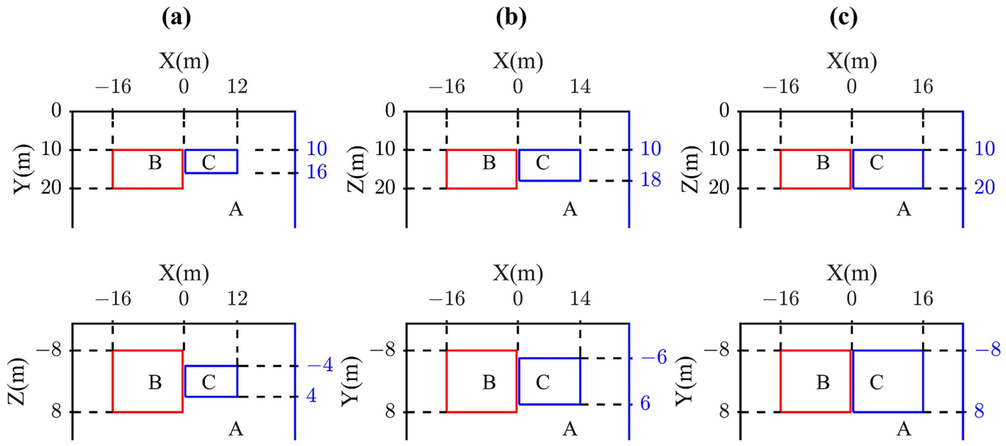
Figure 2 provides a schematic illustration of model evolution, showing representations in the X–Z and X–Y planes for each epoch from left to right. The background host rock A has a resistivity of 100 Ω·m and a polarizability of 0.01. Anomaly B has a resistivity of 1000 Ω·m; a polarizability of 0.01; fixed dimensions of 16 m, 16 m, and 10 m in the X-, Y-, and Z-directions; and a top depth of 10 m. Anomaly C has a resistivity of 10 Ω·m and a polarizability of 0.2, with its top also at a depth of 10 m. The spatial extent of anomaly C progressively increases: at T₁, it measures 12 m, 8 m, and 6 m in the X-, Y-, and Z-directions; at T_2, it expands to 14 m, 12 m, and 8 m in the X-, Y-, and Z-directions; and at T_3, it reaches dimensions of 16 m, 16 m, and 10 m in the X-, Y-, and Z-directions.

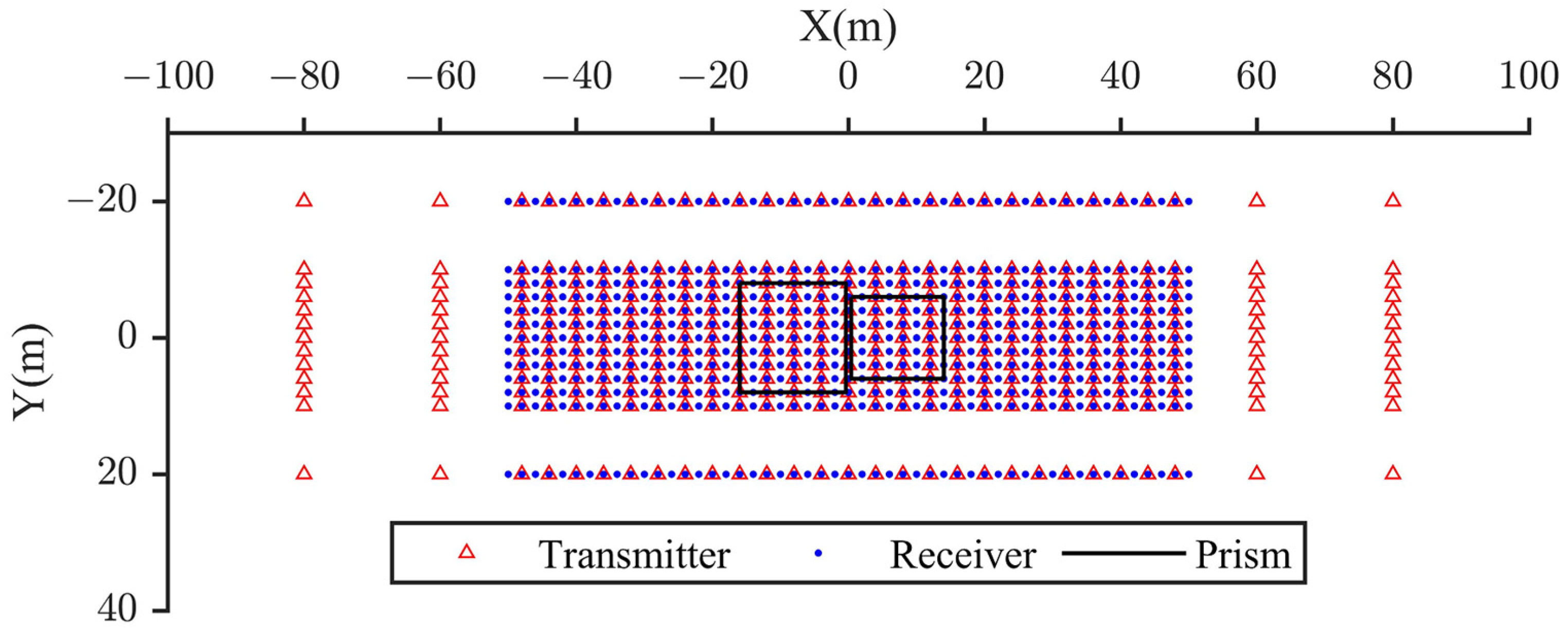
Figure 3 illustrates the survey configuration employed for the time-lapse model. A profiling approach with multiple survey lines was adopted. In this configuration, when a transmitter point on a specific line is energized, only adjacent receiver points on the same corresponding line record the signal. This acquisition geometry closely mimics real-world field data acquisition scenarios.

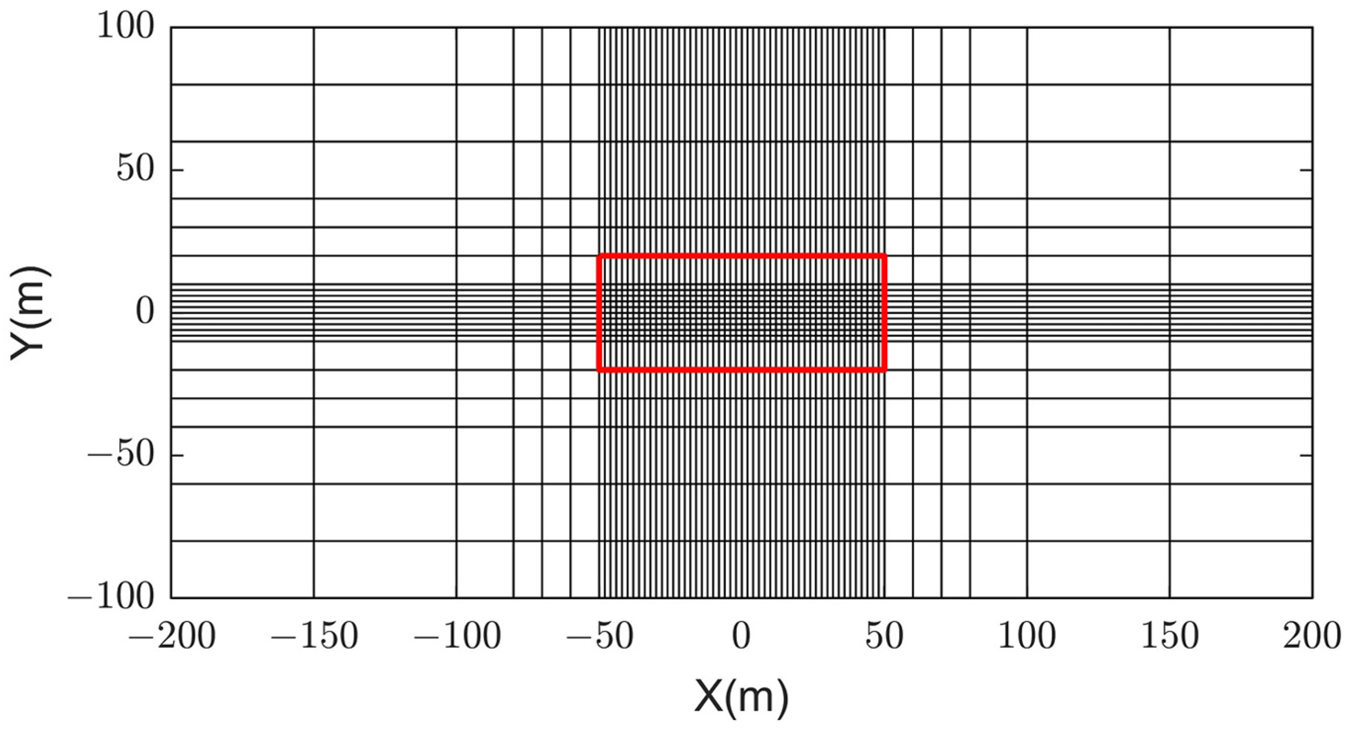
In this study, the finite difference method was employed for forward calculations, necessitating that all transmitting and receiving electrodes be positioned at grid nodes. To minimize the impact of boundaries on forward modeling data, the boundary range is set to exceed three times the observation area. Figure 4 illustrates a schematic diagram of mesh subdivision in the X–Y direction.

To simulate the varying noise levels encountered in practical repeated surveys, Gaussian random noise with amplitudes of 5%, 20%, and 10% was added to the synthetic data for epochs T₁, T₂, and T₃, respectively. After data screening, 18,200 valid data points were obtained for each epoch, yielding a total of 54,600 observed data points across the three epochs.

3.2. Analysis of the Inversion Results

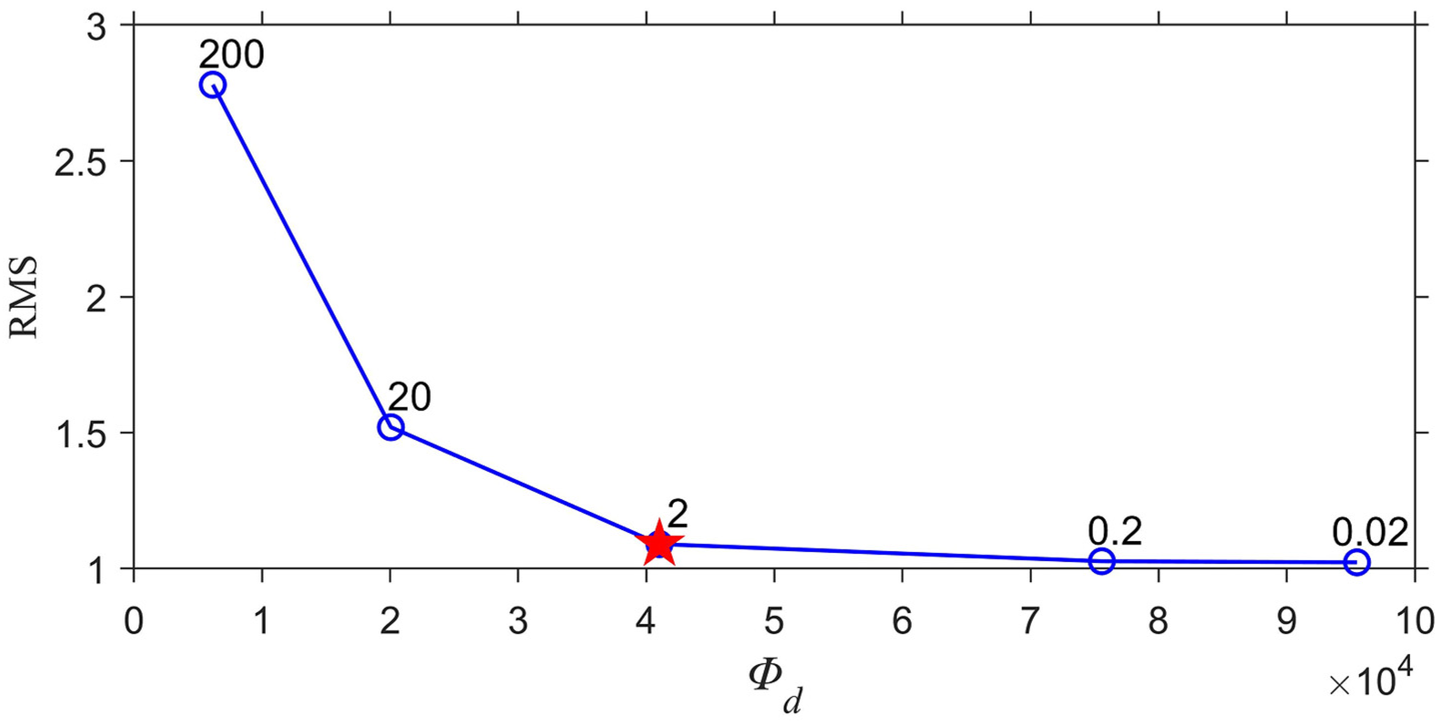
The synthetic data were subjected to three inversion schemes: separate inversion, time-lapse inversion, and time-lapse joint inversion. The method of L-curves was used for calculating the regularization weighting factors. Figure 5 illustrates the selection process for the regularization factor ${\lambda }_m^{\sigma }$ using the L-curve method. Various regularization factors—0.02, 0.2, 2, 20, and 200—were applied to invert the observed data, producing a curve graph of the final RMS value and data misfit term. The optimal regularization factor is indicated by the red five-pointed star at the curve’s inflection point. At this point, the regularization factor ensures that the model term acts as a constraint while the inversion results accurately fit the observed data. In this study, all weight factors were selected using this method, and the final values of ${\lambda }_m^{\sigma }$, ${\lambda }_t^{\sigma }$, ${\lambda }_{cg}^{\sigma }$, ${\lambda }_m^{\eta }$, ${\lambda }_t^{\eta }$, and ${\lambda }_{cg}^{\eta }$ were set to 2, 0.2, 1000, 10, 1, and 2000, respectively.

In this synthetic example, the upper and lower limits of resistivity are predefined. Consequently, the following transformation can be applied to enhance the convergence speed of the inversion process and minimize false anomalies, using conductivity as an example.

$$\begin{array}{cc}{M}_{\sigma }=\mathit{ln}({\displaystyle \frac{\sigma -a}{b-\sigma }}),& a<\sigma <b\end{array},$$

(21)

where $a$ and $b$ represent the upper and lower bounds of conductivity, respectively. In this study, the values of $a$ and $b$ were set to 8 and 1200, respectively. The gradient during the inversion iteration process is:

$$g_{\sigma }=g\cdot {\displaystyle \frac{\left(b-a\right)e^{m_{\sigma }}}{{\left[1+e^{m_{\sigma }}\right]}^2}},$$

(22)

once the inversion is complete, an exponential transformation is applied:

$$\sigma ={\displaystyle \frac{a+b{e}^{m_{\sigma }}}{1+e^{m_{\sigma }}}},$$

(23)

The true conductivity parameters of the underground subdivision unit can be obtained, and the value range corresponding to conductivity from 8 to 1200. This transformation not only enhances the stability of inversion but also reduces its solution space. The same transformation method is applied to the polarizability models.

The methods for calculating ${\mathit{W}}_{d,\sigma }$ and ${\mathit{W}}_{d,\eta }$ are as follows:

$$\left\{\begin{array}{c}{\mathit{W}}_{d,\sigma }={\left({\mathit{D}}_{\mathit{\rho },\mathit{o}\mathit{b}\mathit{s}}\cdot \mathcal{L}\right)}^{-2}\\ {\mathit{W}}_{d,\eta }={\left({\mathit{D}}_{\mathit{\eta },\mathit{o}\mathit{b}\mathit{s}}\cdot \mathcal{L}\right)}^{-2}\end{array}\right.,$$

(24)

where $\mathcal{L}$ is the error level. In this synthesis example, different Gaussian random errors are added to various epochs. Since time-lapse joint inversion requires simultaneous inversion of data from all epochs, it is essential to ensure that data from different epochs carry similar weight during the inversion process. Therefore, the value of $\mathcal{L}$ is uniformly set to 5%.

The final RMS values for the resistivity method under these three inversion modes were 1.87, 1.88, and 1.88, whereas those for TDIP were 1.96, 1.97, and 1.97, respectively. The final RMS values are relatively close, indicating that each approach achieves satisfactory fitting of the observed data.

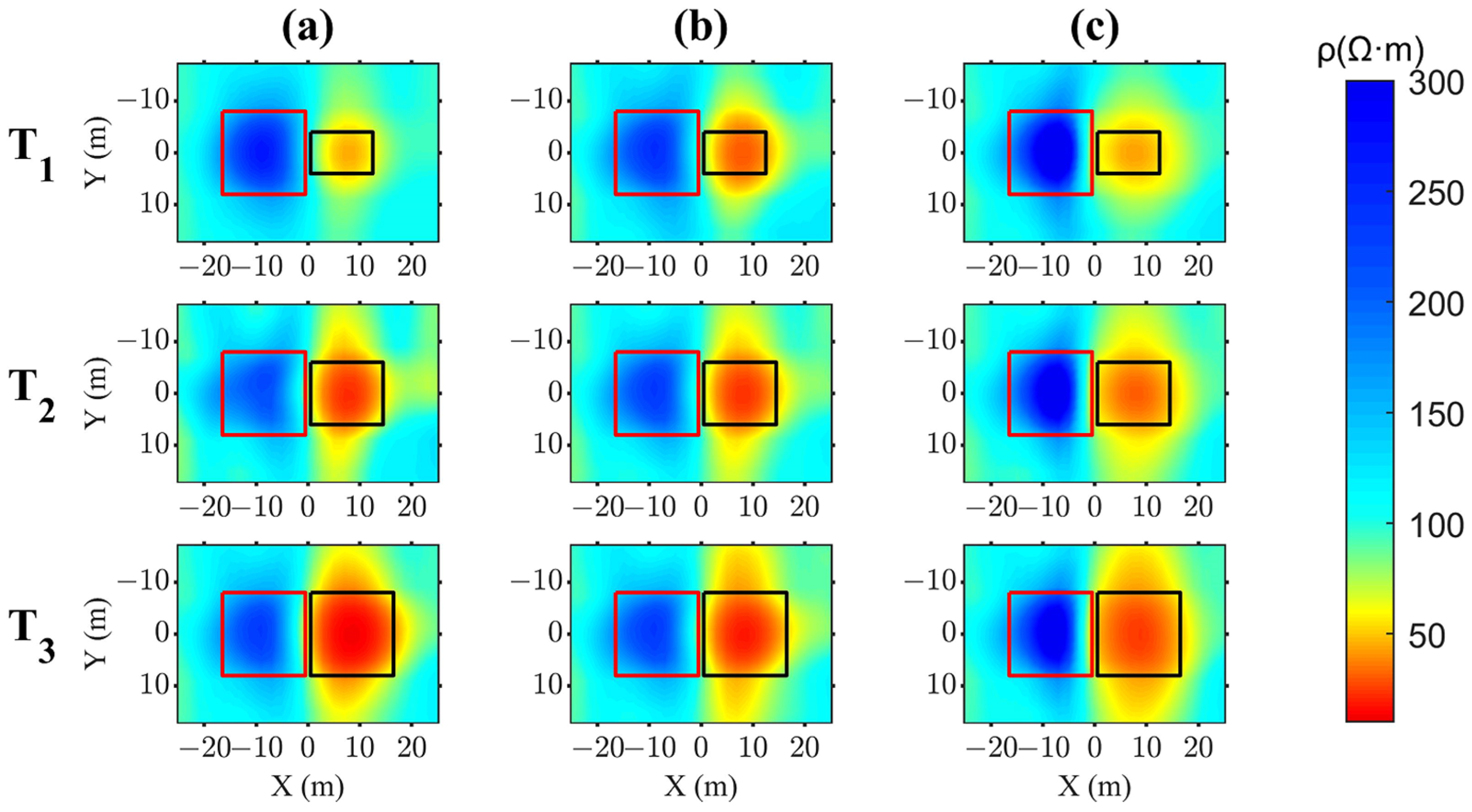
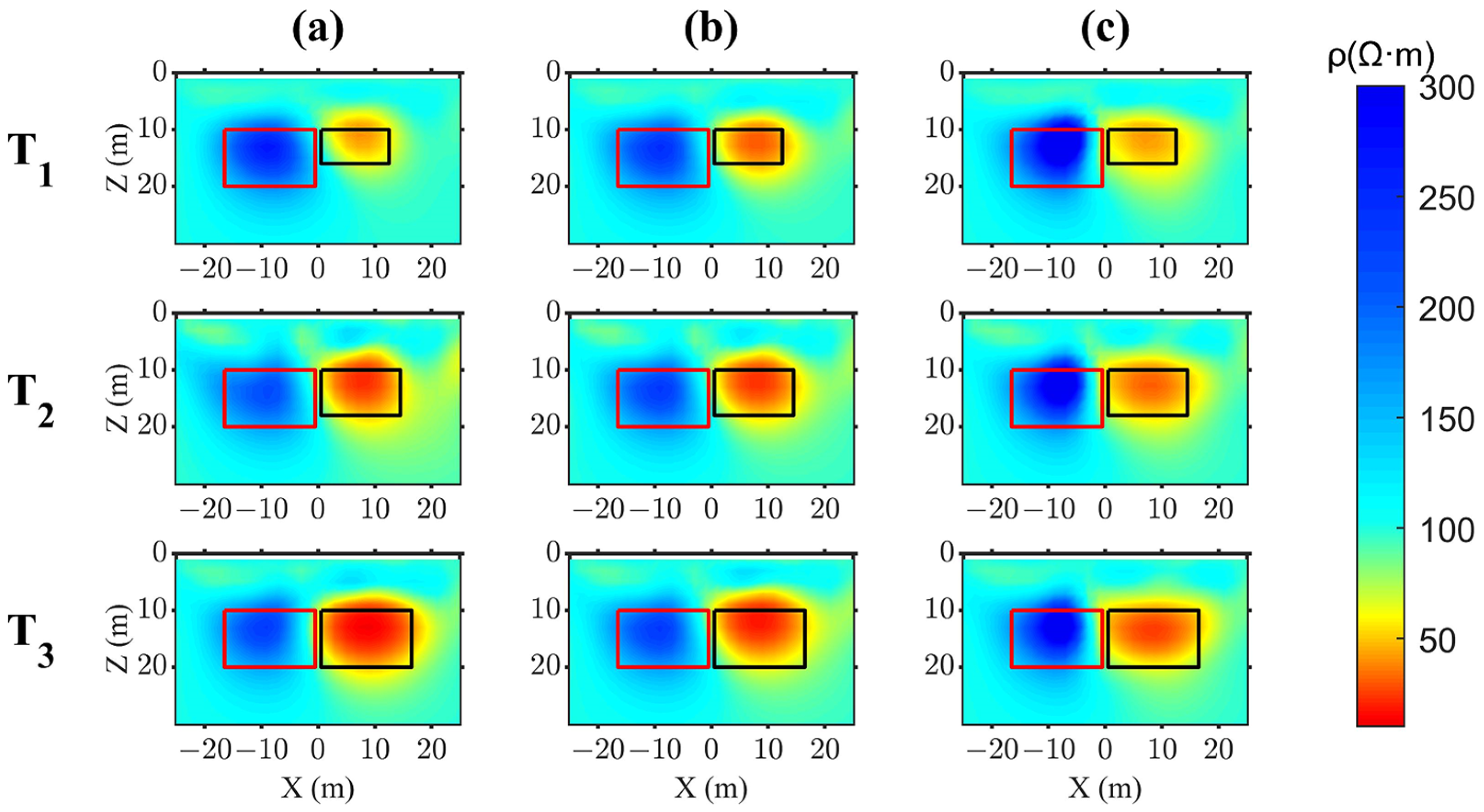
Figure 6 and Figure 7 show the sections at Z = 14 m and Y = 0 m for the resistivity inversion results, respectively. The panels from left to right correspond to the separate inversion, time-lapse inversion, and time-lapse joint inversion results. The red solid lines denote the true boundaries of anomaly B, whereas the black solid lines indicate the true boundaries of anomaly C.

As shown in Figure 6 and Figure 7, the resistivity results from the time-lapse joint inversion outperform those from the alternative inversion schemes. In the separate inversion results at cross-section Z = 14 m and profile Y = 0 m, significant discrepancies exist between the recovered and true anomalies across all three epochs, particularly manifested in the substantially underestimated resistivity of B relative to its true value. Under high noise levels at T₂ and T₃, B exhibits geometric distortion with further reduced resistivity compared with T₁, whereas C shows decreasing resistivity values coinciding with its spatial expansion. Following time-lapse inversion, the resistivity values of both bodies become more temporally consistent, and distortion at T₂ and T₃ is mitigated; however, this introduces new geometric distortion at T₁ while further lowering the resistivity of B. Time-lapse joint inversion yields superior outcomes at Z = 14 m and Y = 0 m, and B and C display more regular geometries and enhanced structural definitions across all epochs. Critically, B’s resistivity increases toward the true value while maintaining a consistent morphology and magnitude throughout T₁, T₂, and T₃, which aligns with the ground truth. Additionally, distortion artifacts are virtually eliminated across all cross-sections, with anomaly boundaries restored to their true model positions.

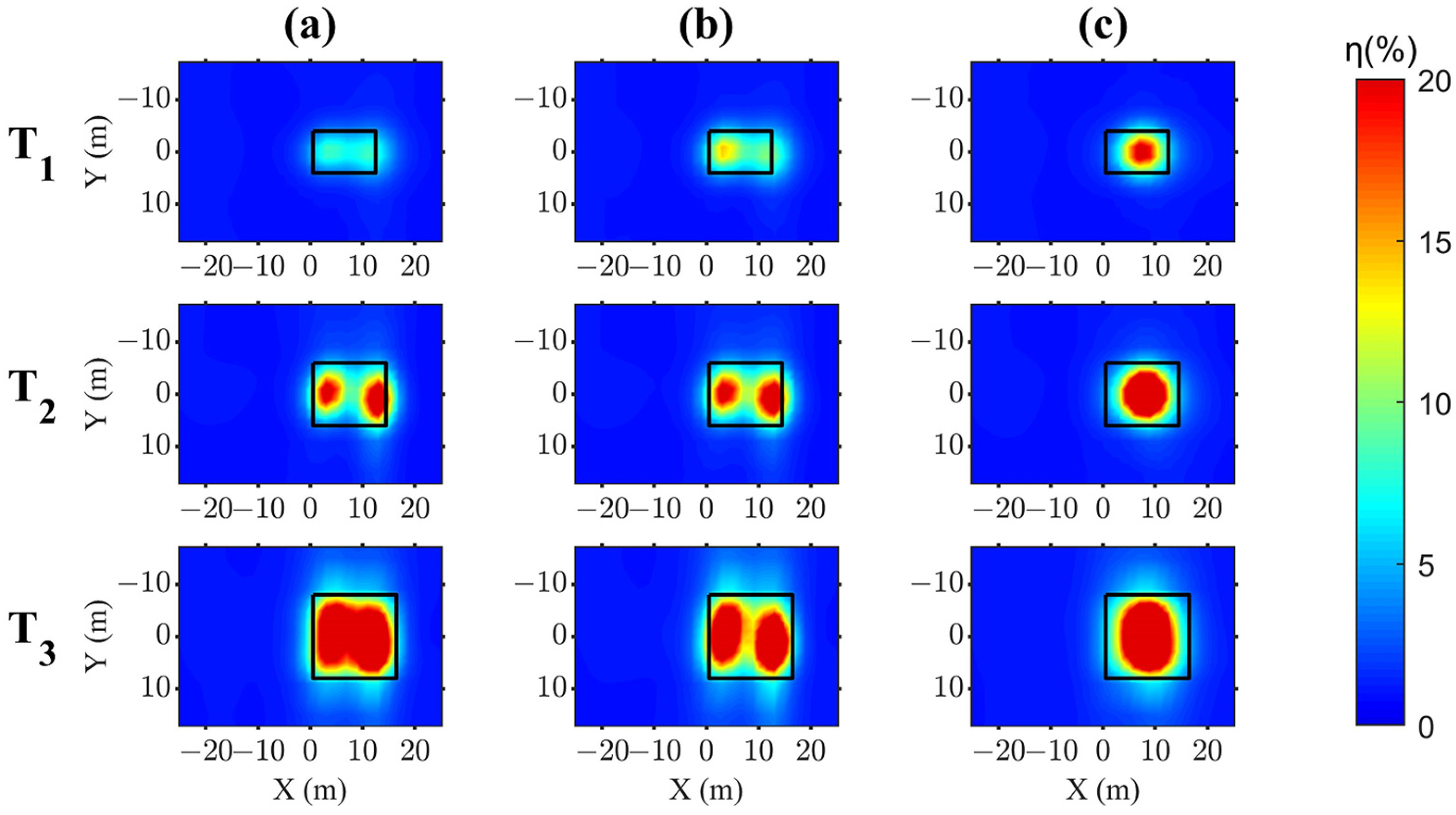
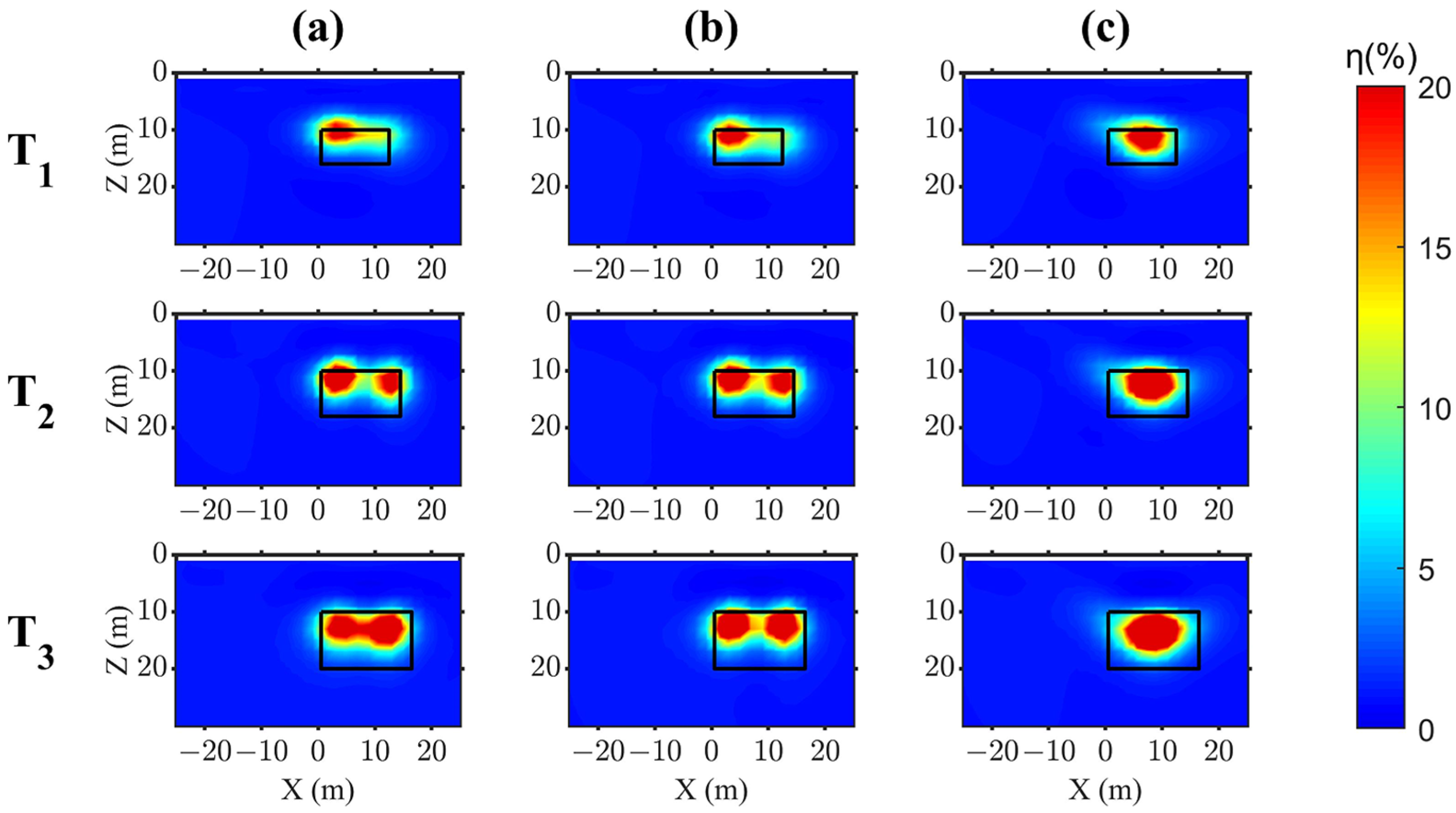
Figure 8 and Figure 9 show the sections at Z = 14 m and Y = 0 m for the polarizability inversion results, respectively. The panels from left to right correspond to the separate inversion, time-lapse inversion, and time-lapse joint inversion results. The black solid lines indicate the true boundaries of anomaly C.

As shown in Figure 8 and Figure 9, both separate and time-lapse polarizability inversions perform poorly because of interference from the left-side high-resistivity anomaly and elevated noise levels, whereas the time-lapse joint inversion yields significantly superior polarizability results. At cross-section Z = 14 m and profile Y = 0 m, separate inversion results in underestimated polarizability for Anomaly C at T₁ relative to its true value, whereas high noise at T₂ deforms C into two separate high-polarizability bodies with emerging distortion at T₃. Time-lapse inversion further degrades performance by splitting C into two distinct anomalies across all epochs. In contrast, time-lapse joint inversion eliminates distortion artifacts throughout all cross-sections, restoring anomaly boundaries to precise alignment with the true model. This approach significantly improves the geometric restoration of C, achieving close resemblance to the true configuration, particularly at cross-section Z = 14 m and profile Y = 0 m, where C returns to its central position, whereas at Z = 14 m in the T₁ epoch, the recovered polarizability values increase toward the ground-truth model value.

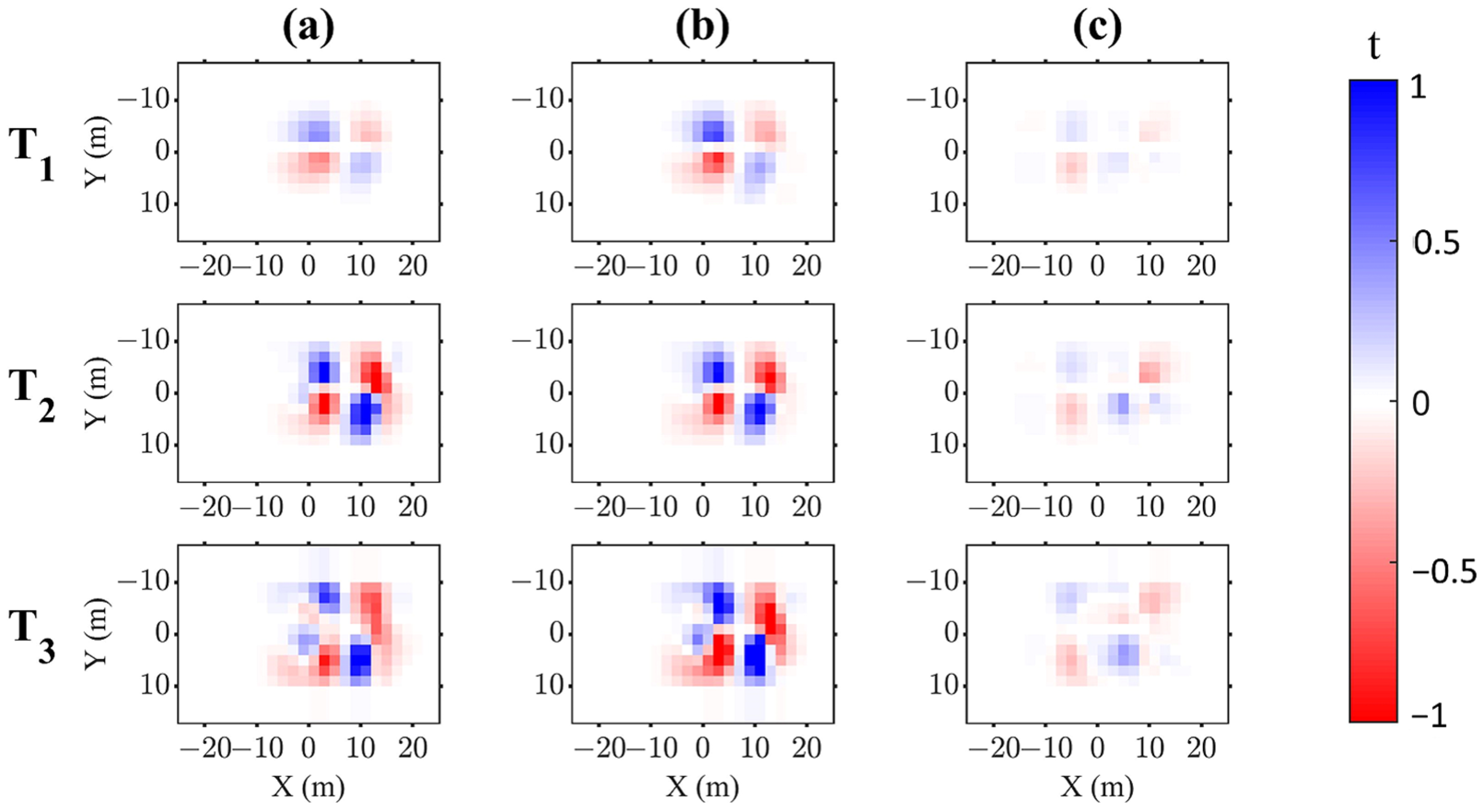
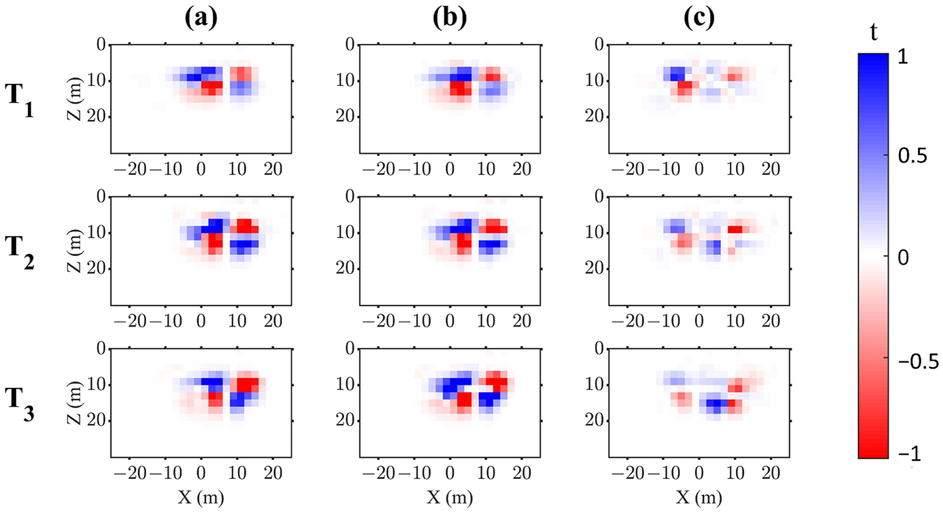
To better demonstrate the structural similarity between the resistivity and polarizability inversion results, we compute the cross-gradient function values according to (9). Figure 10 and Figure 11 display the corresponding cross-gradient distribution maps at cross-section Z = 14 m and profile Y = 0 m for each inversion scheme.

As shown in Figure 10 and Figure 11, separate inversion yields strong cross-gradient magnitudes, which are primarily concentrated within C. In time-lapse inversion, the cross-gradient distribution becomes more spatially extensive with increased magnitude than in separate inversion, indicating that the structural discrepancies between the resistivity and polarizability models become stronger. Notably, time-lapse joint inversion produces cross-gradient values approaching zero, demonstrating significant improvement over the other three inversion schemes.

3.3. Quantitative Analysis

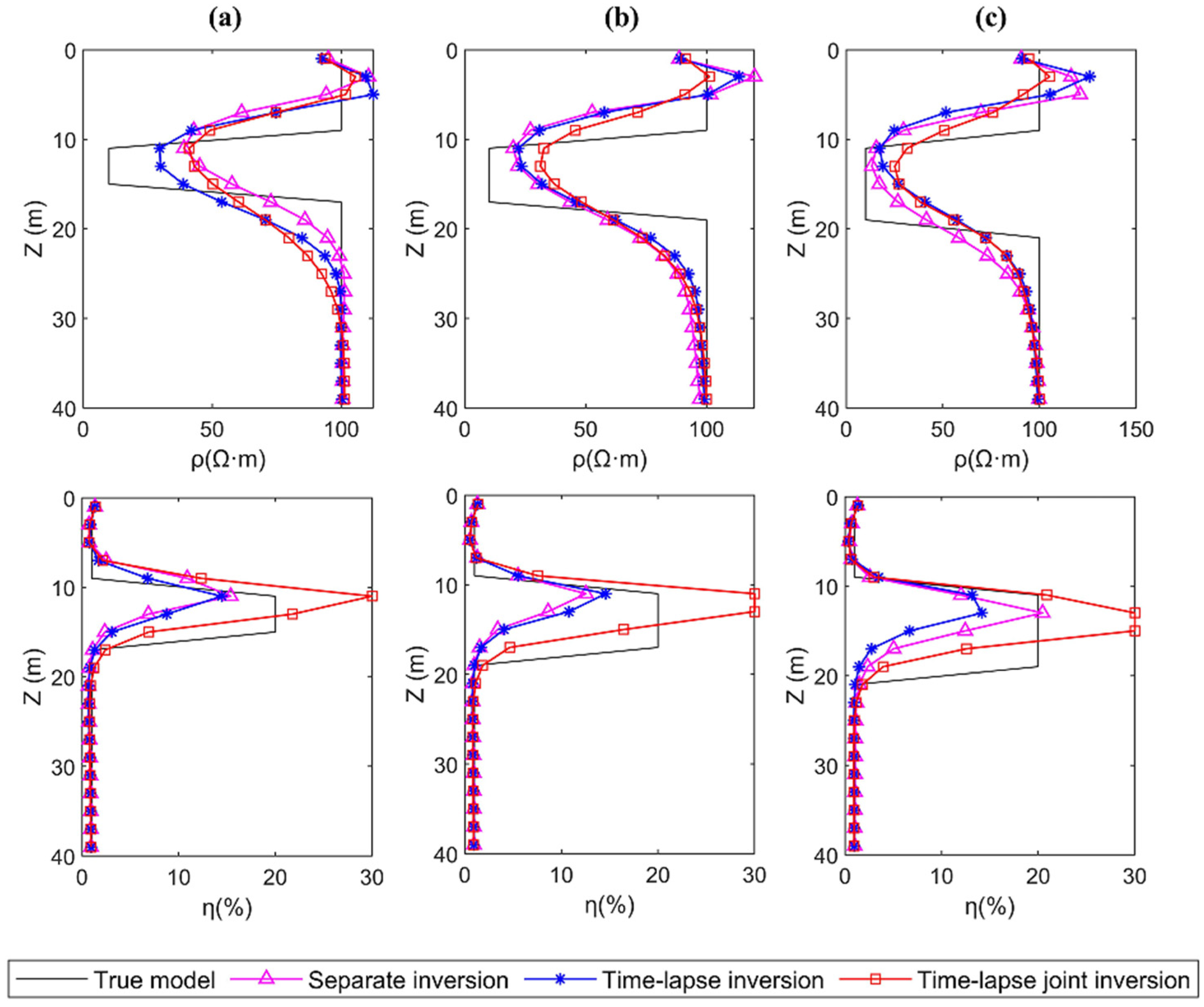
To quantitatively assess the superiority of time-lapse joint inversion, we plotted the curves of resistivity and polarizability with depth for the true model and inversion results at X = 6 m, as shown in Figure 12.

By comparing the resistivity curves of the true model and the inversion results, it becomes evident that, irrespective of the time periods T₁, T₂, or T₃, the resistivity from the time-lapse joint inversion more closely aligns with the true values at the anomalous boundary. Additionally, the position of the minimum resistivity is nearer to the center of the true model. Similarly, when examining the polarizability curves, both separate inversion and time-lapse inversion failed to accurately restore the model’s true values. However, the time-lapse joint inversion yields results that are closer to the true values at the model’s position, with the position also being closer to the center of the true model.

To quantitatively evaluate the role of the cross-gradient term, we introduce the mean cross-gradient value $\overline{t}$ to assess the structural similarity between the resistivity and polarizability inversion results, computed as:

$$\overline{t}={\displaystyle \frac{1}{M_p}}\sqrt{{\sum }_{i=1}^{M_p}\left[(t_x^i{)}^2+(t_y^i{)}^2+(t_z^i{)}^2\right]},$$

(25)

where $M_p$ represents the total number of grid cells underground.

Table 1. Statistics of $\overline{t}$ for resistivity and polarizability inversion results.

Epoch	$\overline{\mathit{t}}$
	Separate Inversion	Time-Lapse Inversion	Time-Lapse Joint Inversion
T1	6.45 × 10−6	1.10 × 10−5	3.53 × 10−6
T2	2.93 × 10−5	2.01 × 10−5	3.17 × 10−6
T3	1.95 × 10−5	3.15 × 10−5	3.01 × 10−6

presents the mean cross-gradient values $\overline{t}$ for each inversion scheme.

Analysis of $\overline{t}$ variations: compared with separate inversion, time-lapse inversion yields increased $\overline{t}$ at the T₁ and T₃ epochs, which is attributed to contamination from the high-noise T₂ epoch, whereas temporal constraints reduce $\overline{t}$ at T₂. Critically, time-lapse joint inversion achieves significantly lower $\overline{t}$ values across all three epochs than both the separate and time-lapse inversion schemes do.

To quantitatively evaluate the performance of time-lapse joint inversion, we introduce the model fitting difference $\delta$ to compute the discrepancies between the true and inverted models. The formulation of $\delta$ is adapted from the methodology established by Moorkamp [20].

$$\delta ={\displaystyle \frac{1}{M_p}}\sqrt{{{\sum }_{i=1}^{M_p}\left({\displaystyle \frac{m_i^{inv}-m_i^{true}}{m_i^{true}}}\right)}^2}$$

(26)

where $m_i^{true}$ represents the true model, $m_i^{inv}$ represents the result of the inverted models, and $M_p$ represents the total number of grid cells underground.

Table 2. Statistics of $\delta$ for resistivity and inversion results.

Parameter	Epoch	$\mathit{\delta }$
		Separate Inversion	Time-Lapse Inversion	Time-Lapse Joint Inversion
	T1	6.14	3.41	3.92
Resistivity	T2	5.65	5.87	5.47
	T3	5.71	10.22	7.92
	T1	0.39	0.45	0.18
Polarizability	T2	0.44	0.48	0.33
	T3	0.81	0.89	0.56

shows the $\delta$ value statistics of the results of separate inversion, time-lapse inversion, and time-lapse joint inversion.

As shown in Table 2, the values of model misfitting differences $\delta$ computed across all inversion schemes reveal distinct performance patterns. For the resistivity results, separate inversion yields elevated $\delta$ values, particularly at T_1, where the limited spatial extent of C impedes accurate recovery. Time-lapse inversion reduces the value of $\delta$ at T₁ through temporal constraints but increases the value of $\delta$ at T₃ due to contamination from T₂’s high noise levels, whereas T₂ remains relatively stable. Compared with time-lapse inversion, time-lapse joint inversion results in a mild increase in model misfit $\delta$ at T₁ but achieves significant reductions in $\delta$ at both T₂ and T₃.

In contrast, the polarizability results show separate inversion producing uniformly high $\delta$ values across epochs. Time-lapse inversion further increases $\delta$ at all time steps due to noise amplification effects, whereas time-lapse joint inversion achieves the lowest recorded $\delta$ values throughout T₁, T₂, and T₃, confirming its greater robustness against both spatial limitations and noise interference than alternative approaches.

4. Discussion

This study involves theoretical research on the time-lapse joint inversion of resistivity and TDIP methods. A three-dimensional time-lapse joint inversion program for the resistivity and TDIP methods is implemented based on the cross-gradient function and time-lapse function constraint theory.

By designing a synthetic time-lapse model, we generate forward responses with varying noise levels to create synthetic datasets. These datasets are subjected to three inversion schemes: separate inversion, joint inversion, and time-lapse joint inversion, followed by comparative analysis. The results demonstrate that while time-lapse inversion improves temporal continuity across epochs compared with separate inversion, it propagates noise contamination to multiple time steps under high-noise conditions, compromising inversion accuracy. In contrast, the proposed time-lapse joint inversion simultaneously ensures temporal continuity and enhances the structural similarity between the resistivity and polarizability models. Crucially, in high-noise scenarios where separate and time-lapse inversions exhibit limited noise suppression, time-lapse joint inversion significantly mitigates noise contamination in recovered models, demonstrating enhanced noise immunity. Overall, the time-lapse joint inversion program for the resistivity and TDIP methods is shown to be reliable and superior.

References

1. Daily, W.; Ramirez, A.; LaBrecque, D.; Nitao, J. Electrical resistivity tomography of vadose water movement. Water Resour. Res. 1992, 28, 1429–1442. [Google Scholar] [CrossRef]
2. Cassiani, G.; Bruno, V.; Villa, A.; Fusi, N.; Binley, A.M. A saline trace test monitored via time-lapse surface electrical resistivity tomography. J. Appl. Geophys. 2006, 59, 244–259. [Google Scholar] [CrossRef]
3. LaBrecque, D.J.; Yang, X. Difference Inversion of ERT Data: A Fast Inversion Method for 3-D In Situ Monitoring. J. Environ. Eng. Geophys. 2001, 6, 83–89. [Google Scholar] [CrossRef]
4. Kim, J.H.; Yi, M.J.; Park, S.G.; Kim, J.G. 4-D inversion of DC resistivity monitoring data acquired over a dynamically changing earth model. J. Appl. Geophys. 2009, 68, 522–532. [Google Scholar] [CrossRef]
5. Hayley, K.; Pidlisecky, A.; Bentley, L.R. Simultaneous time-lapse electrical resistivity inversion. J. Appl. Geophys. 2011, 75, 401–411. [Google Scholar] [CrossRef]
6. Kim, K.J.; Cho, I.K. Time-lapse inversion of 2D resistivity monitoring data with a spatially varying cross-model constraint. J. Appl. Geophys. 2011, 74, 114–122. [Google Scholar] [CrossRef]
7. Karaoulis, M.; Revil, A.; Tsourlos, P.; Werkema, D.D.; Minsley, B.J. IP4DI: A software for time-lapse 2D/3D DC-resistivity and induced polarization tomography. Comput. Geosci. 2013, 54, 164–170. [Google Scholar] [CrossRef]
8. Zhu, D.; Yang, Y.; Wen, L. Three-Dimensional Inversion of the Time-Lapse Resistivity Method on the MPI Parallel Algorithm. Appl. Sci. 2025, 15, 3885. [Google Scholar] [CrossRef]
9. Gallardo, L.A.; Fontes, S.L.; Meju, M.A.; Buonora, M.P.; De Lugao, P.P. Robust geophysical integration through structure-coupled joint inversion and multispectral fusion of seismic reflection, magnetotelluric, magnetic, and gravity images: Example from Santos Basin, offshore Brazil. Geophysics 2012, 77, B237–B251. [Google Scholar] [CrossRef]
10. Gallardo, L.A.; Meju, M.A. Characterization of heterogeneous near-surface materials by joint 2D inversion of dc resistivity and seismic data. Geophys. Res. Lett. 2003, 30, 1658. [Google Scholar] [CrossRef]
11. Gallardo, L.A.; Meju, M.A. Joint two-dimensional DC resistivity and seismic travel time inversion with cross-gradients constraints. J. Geophys. Res. 2004, 109, B03311. [Google Scholar] [CrossRef]
12. Gallardo, L.A.; Meju, M.A. Joint two-dimensional cross-gradient imaging of magnetotelluric and seismic travel time data for structural and lithological classification. Geophys. J. Int. 2007, 169, 1261–1272. [Google Scholar] [CrossRef]
13. Zhu, D.; Tan, H.; Peng, M.; Wang, T. Three-Dimensional Joint Inversion of the Resistivity Method and Time-Domain-Induced Polarization Based on the Cross-Gradient Constraints. Appl. Sci. 2023, 13, 8145. [Google Scholar] [CrossRef]
14. Van der Vorst, H.A. Bi-CGSTAB: A Fast and Smoothly Converging Variant of Bi-CG for the Solution of Nonsymmetric Linear Systems. SIAM J. Sci. Stat. Comput. 1992, 13, 631–644. [Google Scholar] [CrossRef]
15. Li, Y.; Oldenburg, D.W. 3-D inversion of induced polarization data. Geophysics 2000, 65, 1931–1945. [Google Scholar] [CrossRef]
16. Oldenborger, G.A.; Knoll, M.; LaBrecque, D.J. Time-lapse ERT monitoring of an injection with drawal experiment in a shallow unconfined aquifer. Geophysics 2007, 72, 177–187. [Google Scholar] [CrossRef]
17. Miller, C.R.; Routh, P.S.; Brosten, T.R.; McNamara, L.P. Application of Time-Lapse ERT Imaging to Watershed Characterization. Geophysics 2008, 73, 7–17. [Google Scholar] [CrossRef]
18. Yan, Z.; Tan, H.; Peng, M.; Kong, W.; Wu, P. Three-dimensional joint inversion of gravity, magnetic and magnetotelluric data based on cross-gradient theory. Chin. J. Geophys. 2020, 63, 736–752. [Google Scholar]
19. Egbert, G.D.; Kelbert, A. Computational recipes for electromagnetic inverse problems. Geophys. J. Int. 2012, 189, 251–267. [Google Scholar] [CrossRef]
20. Moorkamp, M.; Heincke, B.; Jegen, M.; Roberts, A.W.; Hobbs, R.W. A framework for 3-D joint inversion of MT, gravity and seismic refraction data. Geophys. J. Int. 2011, 184, 477–493. [Google Scholar] [CrossRef]
Figure 1. Flowchart of the three-dimensional time-lapse joint inversion process for resistivity and TDIP methods.
Applsci 15 10016 g001
Figure 2. Schematic illustration of the time-lapse model evolution. From left to right, (ac) represent the models at three different epochs: T1, T2, and T3. The top panels are schematic diagrams in the X–Y direction, and the bottom panels are schematic diagrams in the X–Z direction. A represents background host rock, with a resistivity of 100 Ω·m and a polarizability of 0.01. The red rectangle indicates the location of pipeline B, with a resistivity of 1000 Ω·m and a polarizability of 0.01. The blue rectangle represents the location of the evolving contaminant plume C, with a resistivity of 10 Ω·m and a polarizability of 0.2.
Applsci 15 10016 g002
Figure 3. The survey configuration employed for the time-lapse model. Red circles represent transmitters, blue dots indicate receivers, and the black rectangle shows the projection of the prism onto the surface.
Applsci 15 10016 g003
Figure 4. Schematic diagram of mesh subdivision in the X–Y direction. The red rectangle denotes the distribution range of the receivers.
Applsci 15 10016 g004
Figure 5. The selection process for the regularization factor λ m σ using the L-curve method. The red is the location of the optimal weight factor.
Applsci 15 10016 g005
Figure 6. The inversion results of resistivity at cross-section Z = 14 m. Panels (ac) represent the models of separate inversion, time-lapse inversion, and time-lapse joint inversion, respectively. The top-to-bottom panels represent schematic diagrams at times T1, T2, and T3. The red solid lines denote the true boundaries of anomaly B, whereas the black solid lines indicate the true boundaries of anomaly C.
Applsci 15 10016 g006
Figure 7. The inversion results of resistivity at profile Y = 0 m. Panels (ac) represent the models of separate inversion, time-lapse inversion, and time-lapse joint inversion, respectively. The top-to-bottom panels represent schematic diagrams at times T1, T2, and T3. The red solid lines denote the true boundaries of anomaly B, whereas the black solid lines indicate the true boundaries of anomaly C.
Applsci 15 10016 g007
Figure 8. The inversion results of polarizability at cross-section Z = 14 m. Panels (ac) represent the models of separate inversion, time-lapse inversion, and time-lapse joint inversion, respectively. The top-to-bottom panels represent schematic diagrams at times T1, T2, and T3. The black solid lines indicate the true boundaries of anomaly C.
Applsci 15 10016 g008
Figure 9. The inversion results of polarizability at profile Y = 0 m. Panels (ac) represent the models of separate inversion, time-lapse inversion, and time-lapse joint inversion, respectively. The top-to-bottom panels represent schematic diagrams at times T1, T2, and T3. The black solid lines indicate the true boundaries of anomaly C.
Applsci 15 10016 g009
Figure 10. The cross-gradient maps of the inversion results at cross-section Z = 14 m. Panels (ac) represent the models of separate inversion, time-lapse inversion, and time-lapse joint inversion, respectively. The top-to-bottom panels represent schematic diagrams at times T1, T2, and T3.
Applsci 15 10016 g010
Figure 11. The cross-gradient maps of the inversion results at profile Y = 0 m. Panels (ac) represent the models of separate inversion, time-lapse inversion, and time-lapse joint inversion, respectively. The top-to-bottom panels represent schematic diagrams at times T1, T2, and T3.
Applsci 15 10016 g011
Figure 12. The curves of resistivity and polarizability with depth for the true model and inversion results at X = 6 m. Panels (ac) represent curves at times T1, T2, and T3. The top panels represent curves of resistivity. The bottom panels represent curves of polarizability.
Applsci 15 10016 g012