Influence of Additive Manufacturing Printing Parameters via LPBF on the Mechanical Strength of Metallic Materials: Numerical Analysis by Gurson-Based Model

Abstract

This paper investigates the influence of initial porosity and its evolution on the mechanical behavior of metallic materials manufactured by additive manufacturing (AM), using the Gurson model to predict the initiation and propagation of damage in specimens produced via Laser Powder Bed Fusion (LPBF). The methodology combines experimental uniaxial tensile tests, numerical simulations based on the Gurson model, and the parametric identification method (PIP) to calibrate constitutive parameters (${\sigma }_{y0}$, ${\sigma }_{\infty }$, $\delta$, $\xi$). The specimens, made of AlSi10Mg with different printing directions (horizontal and vertical) and porosity levels, were evaluated to determine the relationship between density, anisotropy, and mechanical properties. The experimental results revealed that vertical printing accelerates fracture due to the concentration of stresses at the interfaces between layers, while the numerical simulations, compared with the von Mises model, showed greater accuracy of the Gurson model in predicting damage in porous materials. The analysis of porosity evolution highlighted the impact of void size and spacing on coalescence and ductility. The proposed methodology was validated, establishing a useful approach for evaluating the mechanical behavior of materials manufactured by AM. This work contributes to the advancement of the design of lightweight and resistant components, with applications in sectors such as aerospace and automotive, and suggests directions for future studies, including the investigation of other alloys and dynamic loading conditions.

1. Introduction

Porosity is a cavity-shaped defect which grows in volume as the damage evolves [1]. Predicting the behavior of this cavity as the damage evolves in different directions is of fundamental importance in correctly predicting the onset of fracture in ductile materials.

Accordingly, different types of manufacturing produce different volume fractions of cavities in the material’s microstructure, altering the density and mechanical strength of manufactured metallic materials [2]. An example of this is weight reduction in vehicles, aeronautics, and even industrial structures, without compromising performance or market competitiveness, by incorporating design criteria based on determining the ideal moment for damage initiation.

The AlSi10Mg alloy is the material of choice in applications requiring high performance, such as aerospace turbines and orthopaedic implants. When manufactured by LPBF, its microstructure exhibits unique characteristics, influenced by process parameters, such as laser power and scanning speed (see Figure 1).

Research such as that by [3] has shown that laser energy density directly affects pore formation and grain morphology, while [4] has investigated the effects of post-processing heat treatments on reducing defects and improving mechanical properties.

In the current context, in addition to durability, weight reduction has been introduced as a demand in all competitive manufacturing environments, due not only to technological advances but also to the growth of policies to reduce waste and GGEs (greenhouse gas emissions), reinforcing the sustainable bias and establishing itself as the current paradigm [5]. An example of this is the automotive industry, which has been incessantly searching for materials that can reduce vehicle weight without compromising safety and performance.

In aviation, for example, weight reduction has come with the introduction of materials such as aluminum and, more recently, aluminum alloys and carbon-based composites, making it possible to build planes that consume less fuel and are more efficient. Each advance in the weight reduction of metallic materials has not only improved performance in their respective areas but has also opened up new possibilities for the development of emerging technologies.

One of the main problems is porosity, which can arise from trapped gas bubbles, a lack of fusion between layers, or inadequate process parameters [6]. These pores act as stress concentrators, compromising essential mechanical properties, such as tensile strength, ductility, and fatigue resistance, which can lead to premature failure in critical applications [7].

To characterize the mechanical behavior of porous materials, the Gurson model emerged as a fundamental tool. Later studies, such as those by [8], improved the model by introducing parameters that describe the nucleation and coalescence of voids.

This work seeks to measure the initial porosity and the evolution of damage in materials from additive manufacturing and evaluate the relationship between the reduction in density and the conservation of acceptable mechanical properties for metallic materials.

The specific objectives are as follows:

• Perform numerical analysis of specimens manufactured via AM, considering the Gurson constitutive model;
• Extract the maximum stress and displacement values for each specimen modeled, considering porosity;
• Implement an iterative routine to find the critical parameters for the model;
• Compare different volume fractions of voids and their distributions with the mechanical behavior of the material;
• Validate the methodology by establishing a pattern of material behavior due to variation in printing direction and density by AM.

2. Theoretical Basis

AM emerged in the 1980s, when stereolithography began to be used commercially on polymeric materials [9]. Unlike traditional subtractive methods, AM allows the production of complex geometries with less material waste and is widely used in sectors such as aerospace, biomedical, and automotive industries. Its main advantages include part customization, weight reduction, and design flexibility, meeting demands for energy efficiency and sustainability [10].

Figure 2 shows some of the most common techniques for 3D printing metal parts, most of which use metal material in powder form and a laser or electric arc as the source of the melting energy. In this work, LPBF (Laser Powder Bed Fusion) is a process that falls within the processes highlighted in yellow.

Each of the manufacturing techniques has inherent advantages and disadvantages, such as productivity, repeatability, geometric flexibility, and surface quality. LPBF is characterized by medium productivity, good repeatability, and medium to high surface quality. However, two important aspects drastically affect the mechanical properties of the components. Internal stresses resulting from steep temperature gradients and high cooling rates during processing need to be taken into account when evaluating the performance of parts manufactured from any metal powder using LPBF [11].

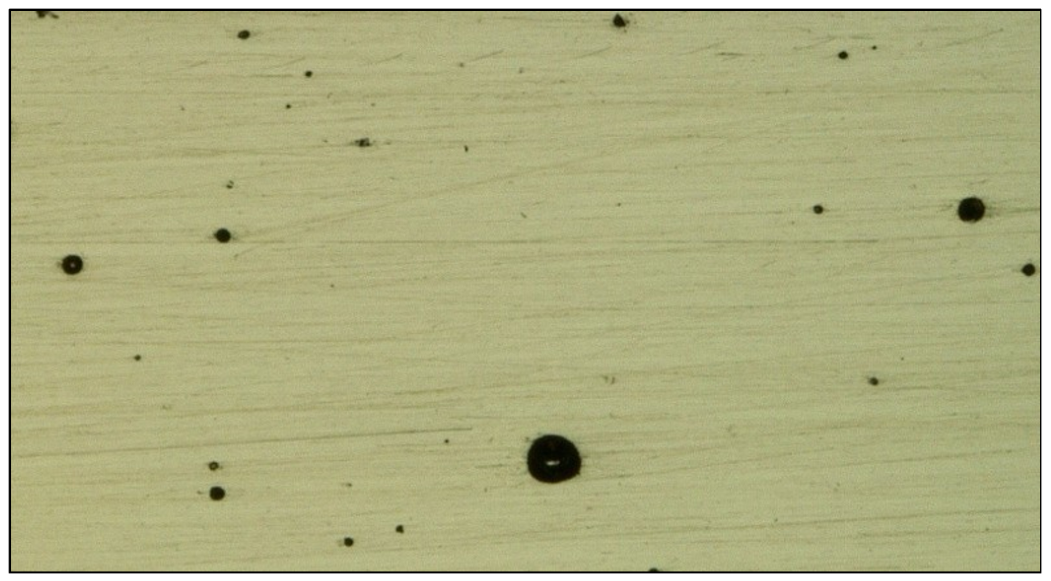
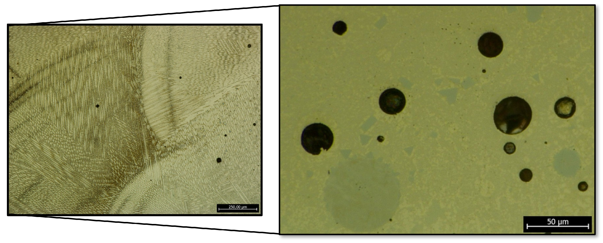
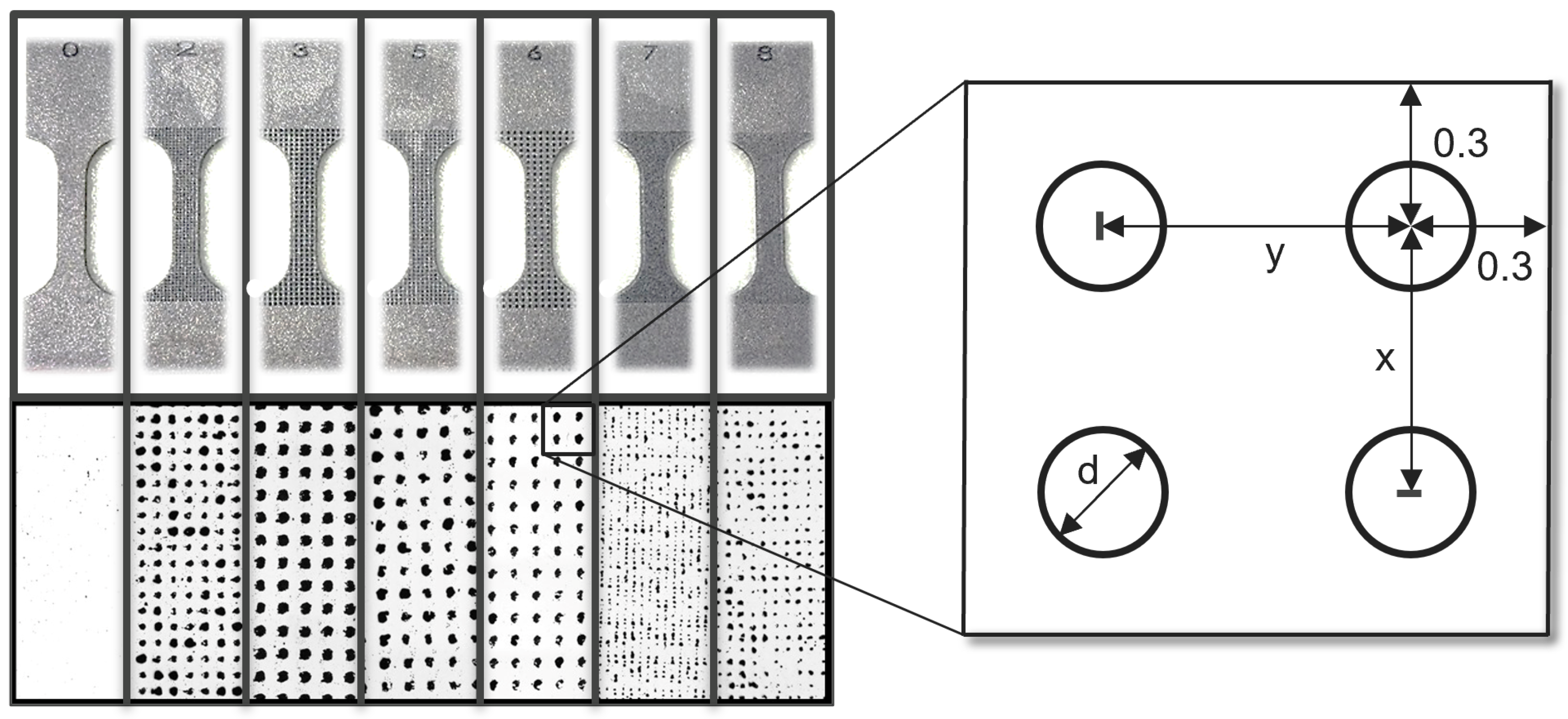
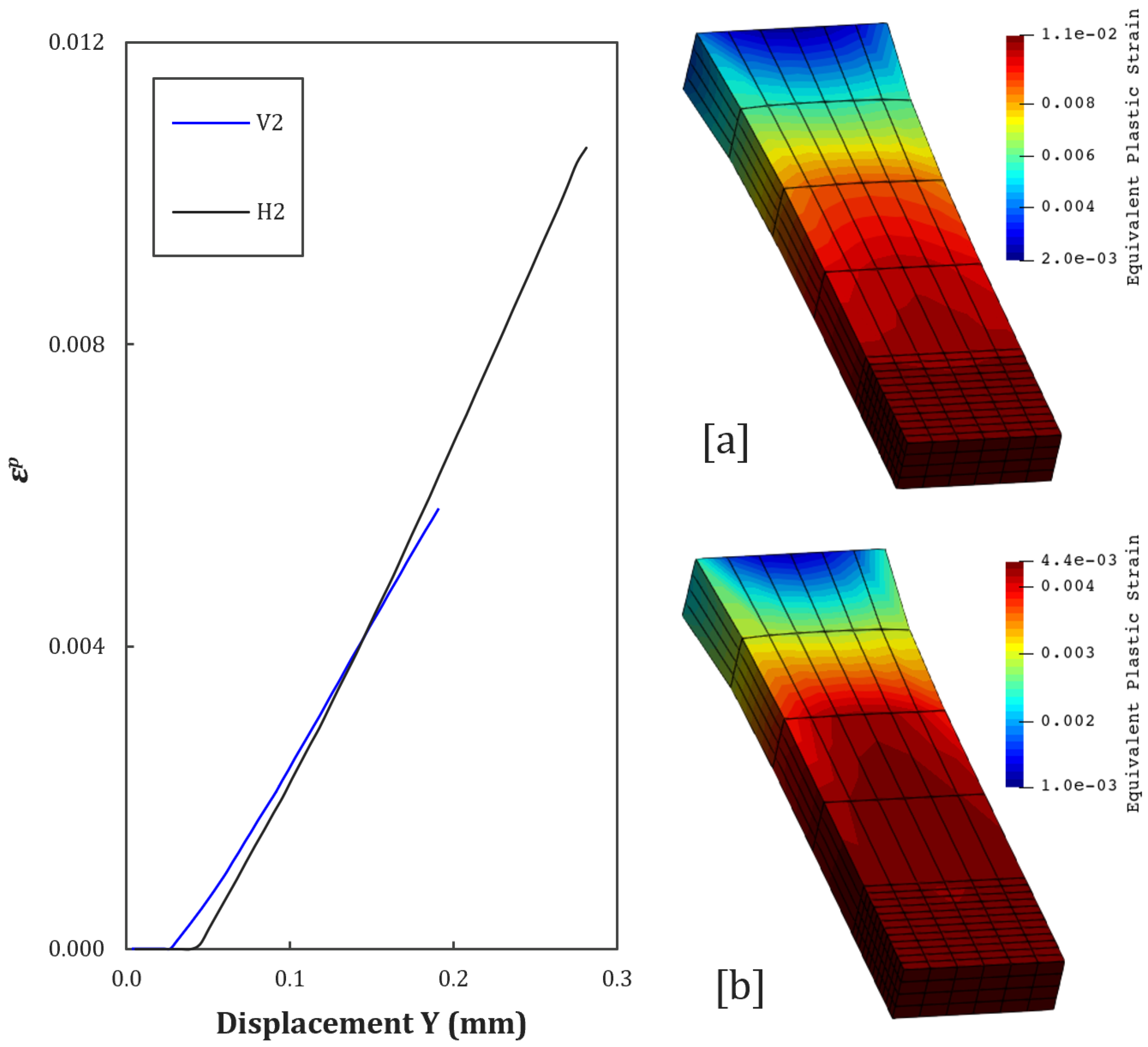
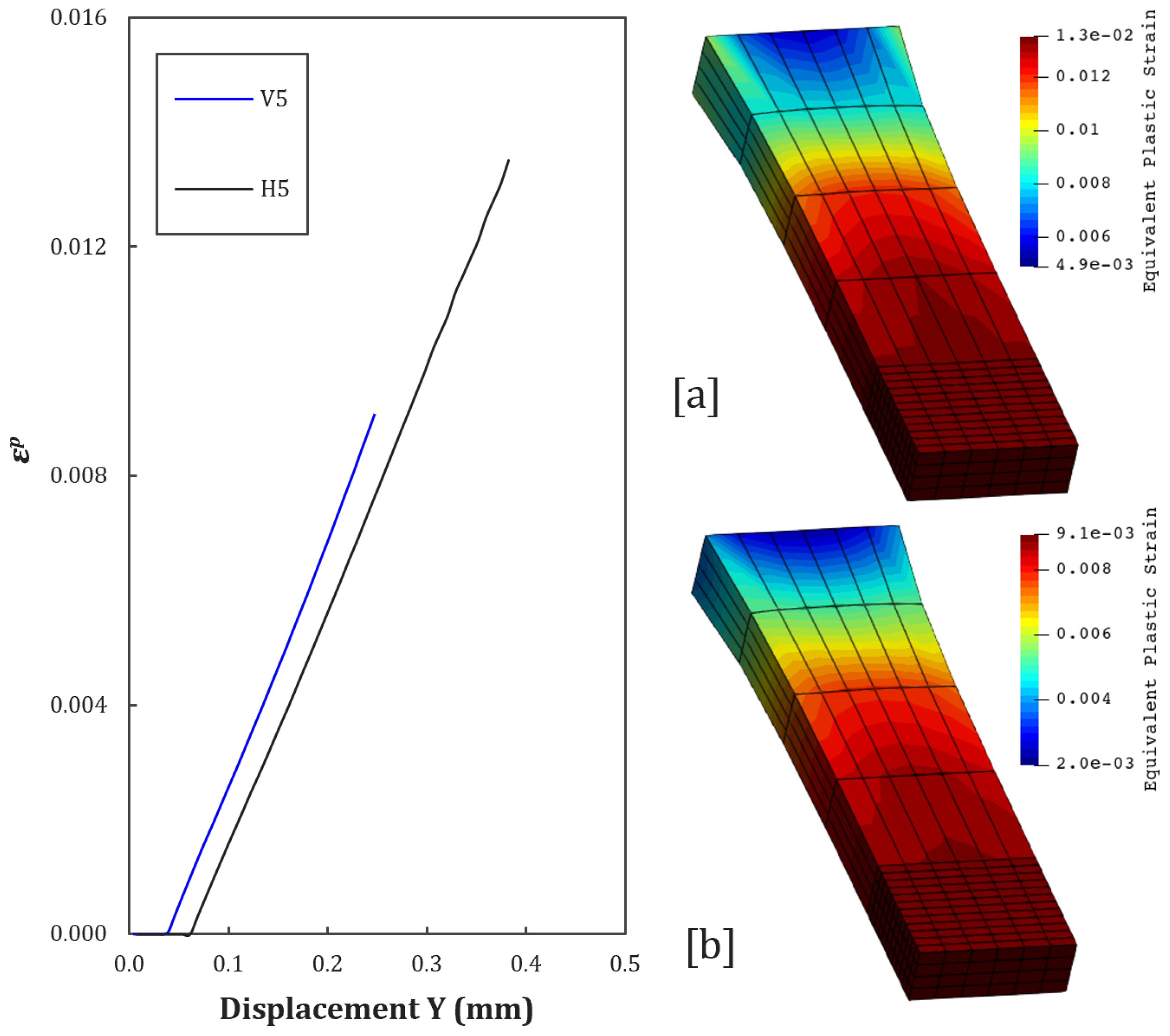
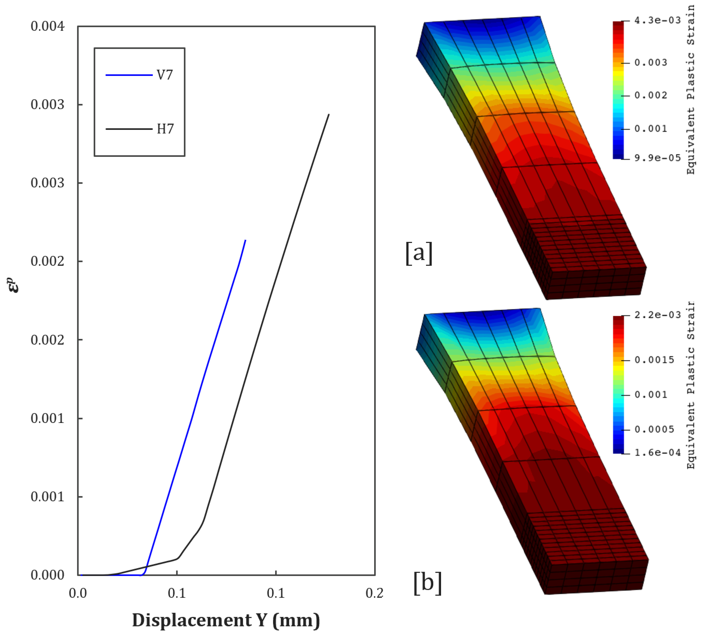
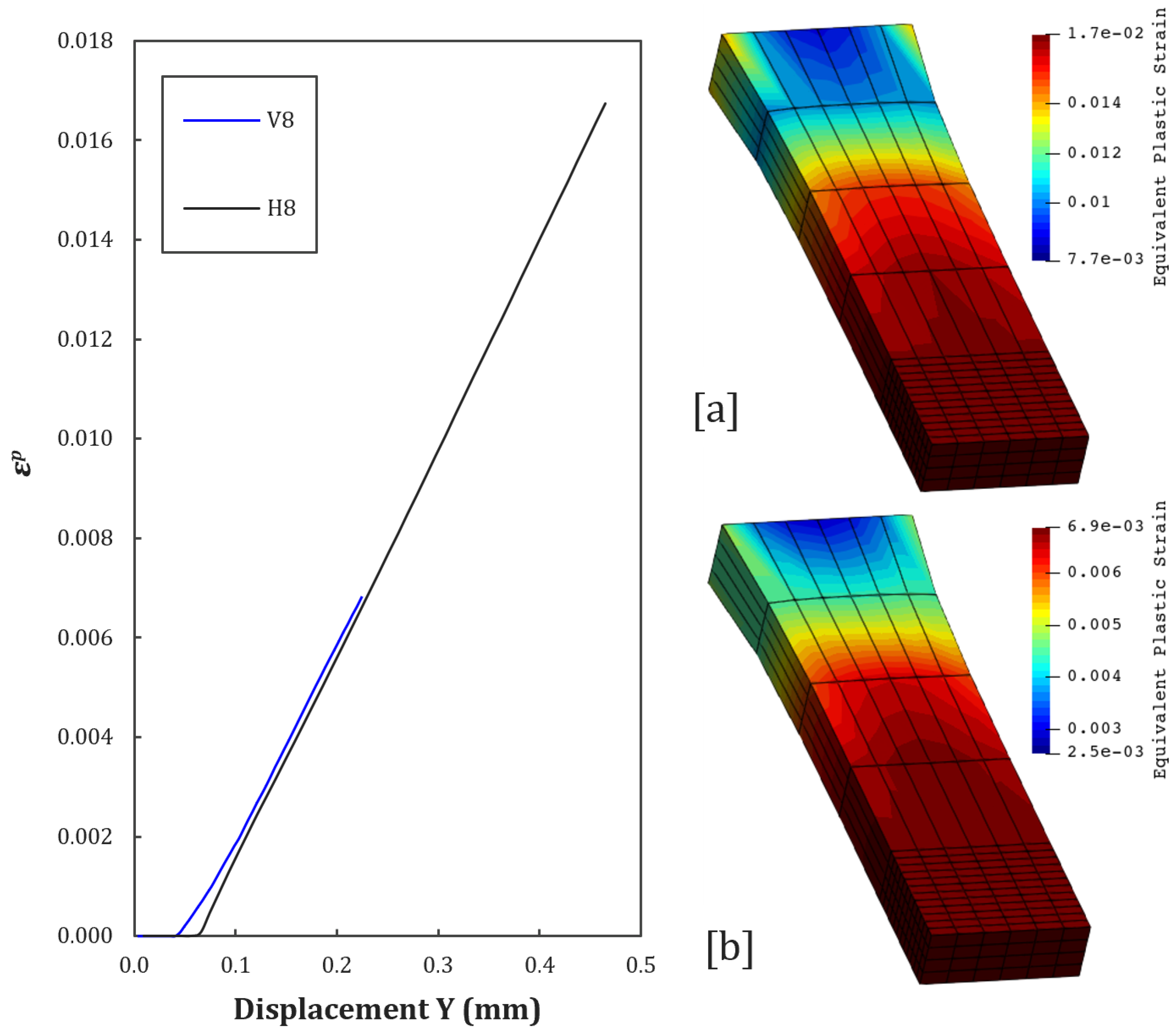
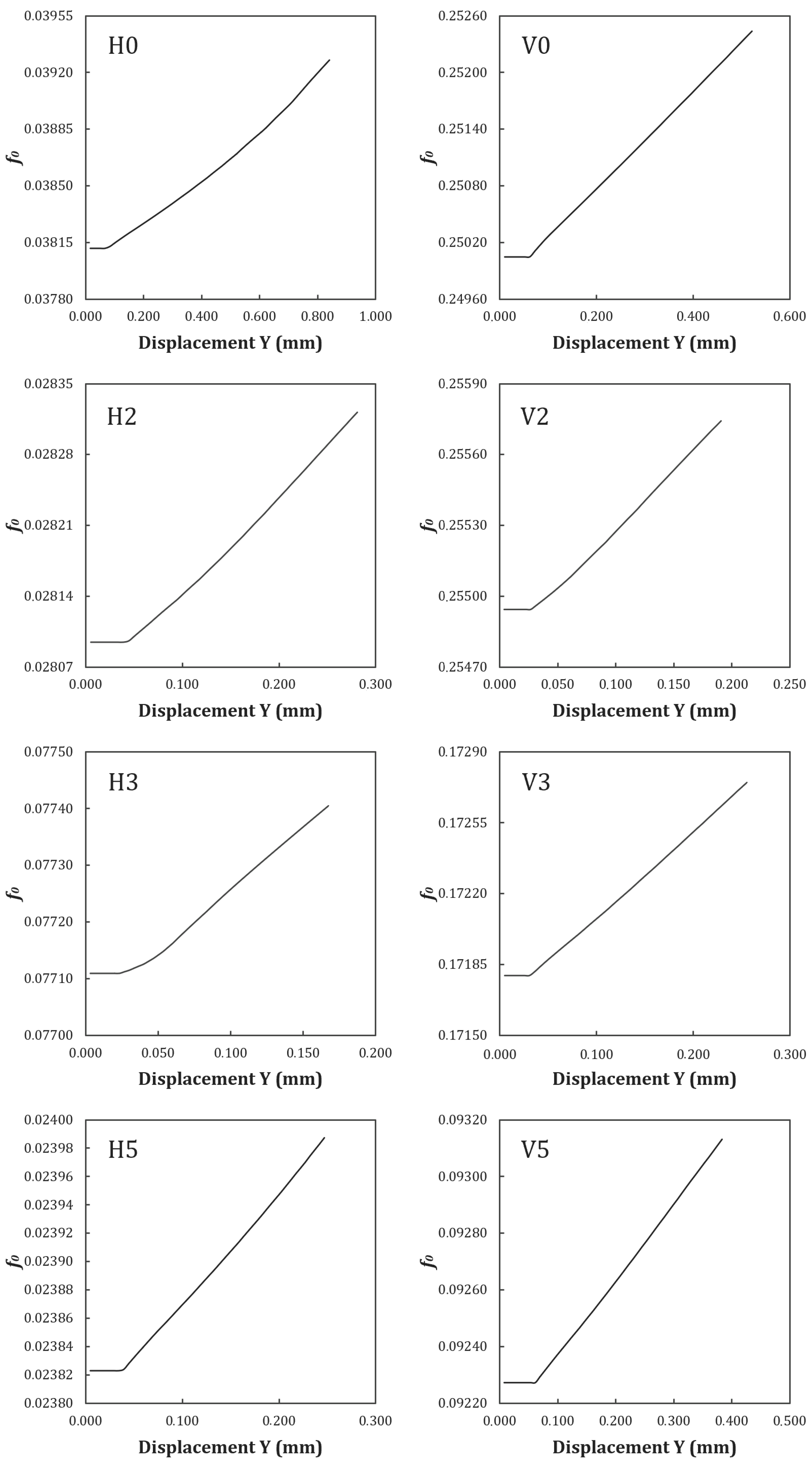
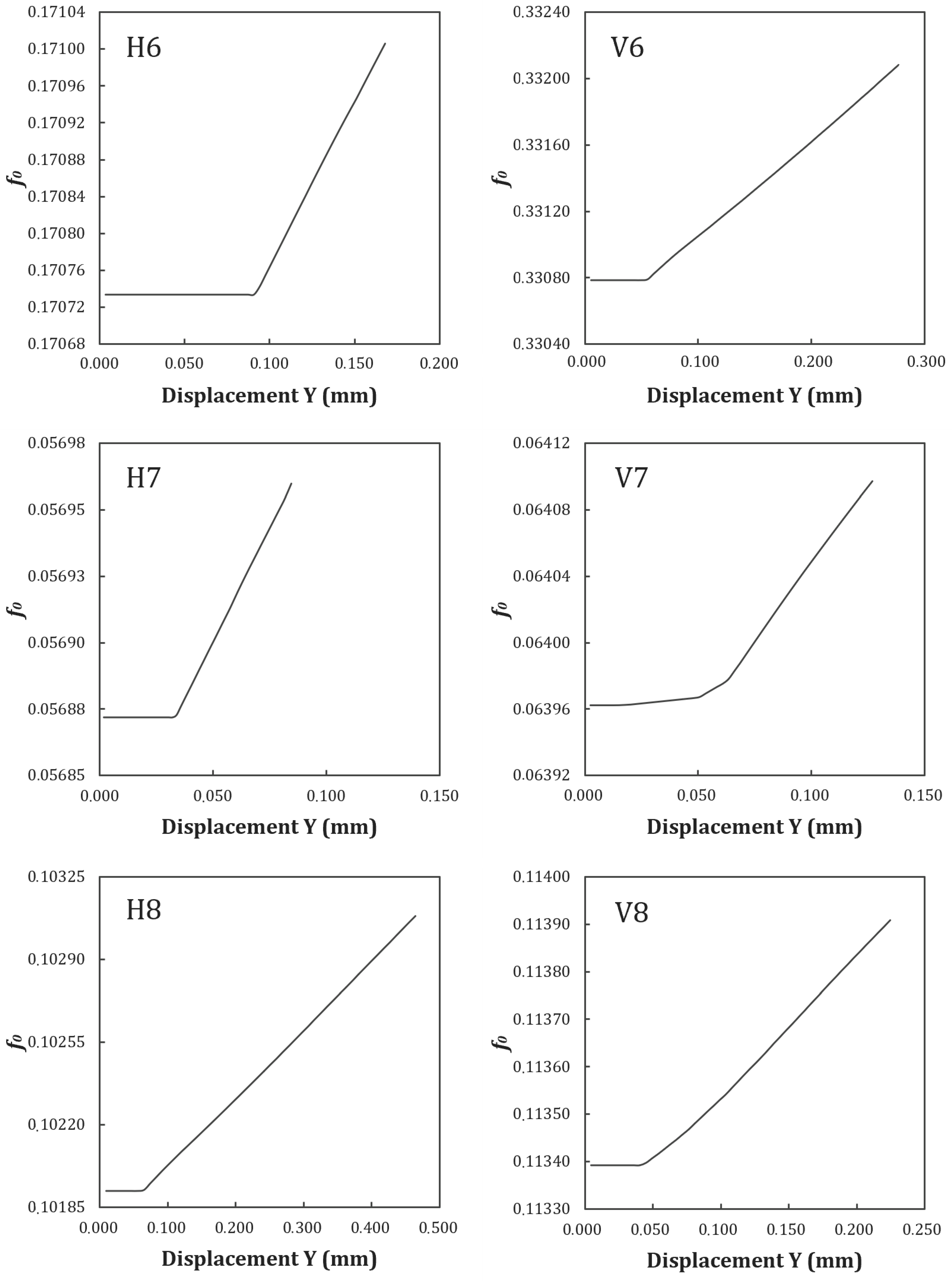
Another major disadvantage related to LPBF is the occurrence of pores in the volume of LPBF-processed parts. These pores arise from process-induced defects originating from initial powder contamination, evaporation, or local voids after the printing of the powder layer. Eventually, these pores act as stress risers and lead the part to failure, especially under fatigue loading. At the time of writing, these pore-like defects cannot be completely avoided.

The aluminum alloy, AlSi10Mg, is a promising candidate for parts manufactured by LPBF, since its use has increased for industrial applications. Consequently, studies focusing on LPBF-processed AlSi10Mg are widely available, however, detailed studies on the combined influence of build orientation and porosity are still lacking.

However, AM faces critical challenges related to the microstructural quality of materials. Among the most common defects is porosity, caused by gas bubbles trapped during material fusion, a lack of fusion between layers, or inadequate process parameters. The presence of pores acts as a stress concentrator, reducing the mechanical strength, ductility, and durability of the parts (see Figure 3). In structural applications, where material integrity is essential, porosity can lead to premature failure under static or cyclic loads.

In this context, the Gurson model is a fundamental tool for characterizing the behavior of materials manufactured by AM. Developed to describe the influence of micro voids on mechanical response, the model explicitly incorporates pore volume fraction (f) and hydrostatic pressure (p) into the flow function. This makes it possible to predict not only the growth of pre-existing voids but also their coalescence under loading, critical aspects for materials with a heterogeneous microstructure.

2.1. Mathematical Model and Numerical Strategy

2.1.1. Gurson’s Model

In the Gurson model, the effective stiffness of the material is reduced in proportion to the fraction of voids, making it more susceptible to deformation even under moderate loads [12].

Additive decomposition of deformation:

$$ϵ={ϵ}^e+{ϵ}^p.$$

(1)

Hooke’s law:

$$\sigma ={(D^e:ϵ)}^e.$$

(2)

Yield function:

$$\varphi =J_2\left(\mathbf{S}\right)-{\displaystyle \frac{1}{3}}\left[1+f^2-2fcosh\left({\displaystyle \frac{3p}{2{\sigma }_y}}\right)\right]{\sigma }_y^2.$$

(3)

Plastic strain law:

$${\dot{ϵ}}^p=\gamma {\displaystyle \frac{\partial N}{\partial \sigma }}=\dot{\gamma }\sqrt{S:S+{\displaystyle \frac{1}{3}}{\left[f{\sigma }_{y}sinh\left({\displaystyle \frac{3p}{2{\sigma }_y}}\right)\right]}^2}$$

(4)

$$\dot{R}=\dot{\gamma }{\displaystyle \frac{fpsinh\left(\frac{3p}{2{\sigma }_y}\right)+\frac{2}{3}[1+f^2-2fcosh\left(\frac{3p}{2{\sigma }_y}\right)]{\sigma }_y^2}{(1-f)}}$$

(5)

$$\dot{f}={\dot{f}}^G=(1-f){ϵ}_v^p$$

(6)

$${ϵ}_v^p=\dot{\gamma }{\sigma }_{y}sinh\left({\displaystyle \frac{3p}{2{\sigma }_y}}\right).$$

(7)

Loading and unloading criteria:

$$\dot{\gamma }\ge 0;\varphi \le 0;\dot{\gamma }\varphi =0.$$

(8)

The core of the model lies in the yield function, which defines the threshold between elastic and plastic behavior [13]. While von Mises uses an exclusive dependence on the second invariant of the deviatoric stress tensor $J_2$, Gurson introduces an additional term that couples hydrostatic pressure (p) and porosity f. The second term proportional to $sinh\left({\displaystyle \frac{3p}{2{\sigma }_y}}\right)$ is also unique to Gurson’s model and represents the plastic expansion induced by the voids. This mechanism is crucial for modeling porous materials, where plasticity not only distorts the metal matrix but also increases the volume of the material due to the expansion of cavities.

2.1.2. The von Mises Stress

The $\sigma$ stress tensor is made up of two parts, one deviatoric and the other hydrostatic [1].

$$\sigma =\mathbf{S}+p\mathbf{I},$$

(9)

where S represents deviatoric stress tensor, p is the hydrostatic pressure and I is the identity tensor of 2nd order. Since the hydrostatic pressure is a function of the deviatoric stresses, we have the invariants of the stress tensor $I_1$, $I_2$, $I_3$:

$$I_1=tr\left(\sigma \right)$$

(10)

$$I_2={\displaystyle \frac{1}{2}}\left\{{\left[tr\left(\sigma \right)\right]}^2-tr\left({\sigma }^2\right)\right\}$$

(11)

$$I_3=det\left(\sigma \right).$$

(12)

For the deviatoric tensor, the first invariant is equal to zero, as it has no volumetric part by definition, so the invariants of the deviatoric tensor $J_2$ and $J_3$ [14] are as follows:

$$J_2={\displaystyle \frac{1}{2}}\mathbf{S}:\mathbf{S}$$

(13)

$$J_3=det\left(\mathbf{S}\right).$$

(14)

As a function of the second invariant of the deviatoric tensor, the equivalent von Mises stress can be expressed as

$$q=\sqrt{3J_2}.$$

(15)

Taking the initial porosity as zero in Equation (3) ($f_0=0$), it is clear that the von Mises model is re-established in Equation (15). Thus, it is stated that the degradation of the mechanical properties of any material can be modeled by the von Mises model constituted by the function of pre-existing micro voids, or those that may form in the material matrix, as established by Gurson.

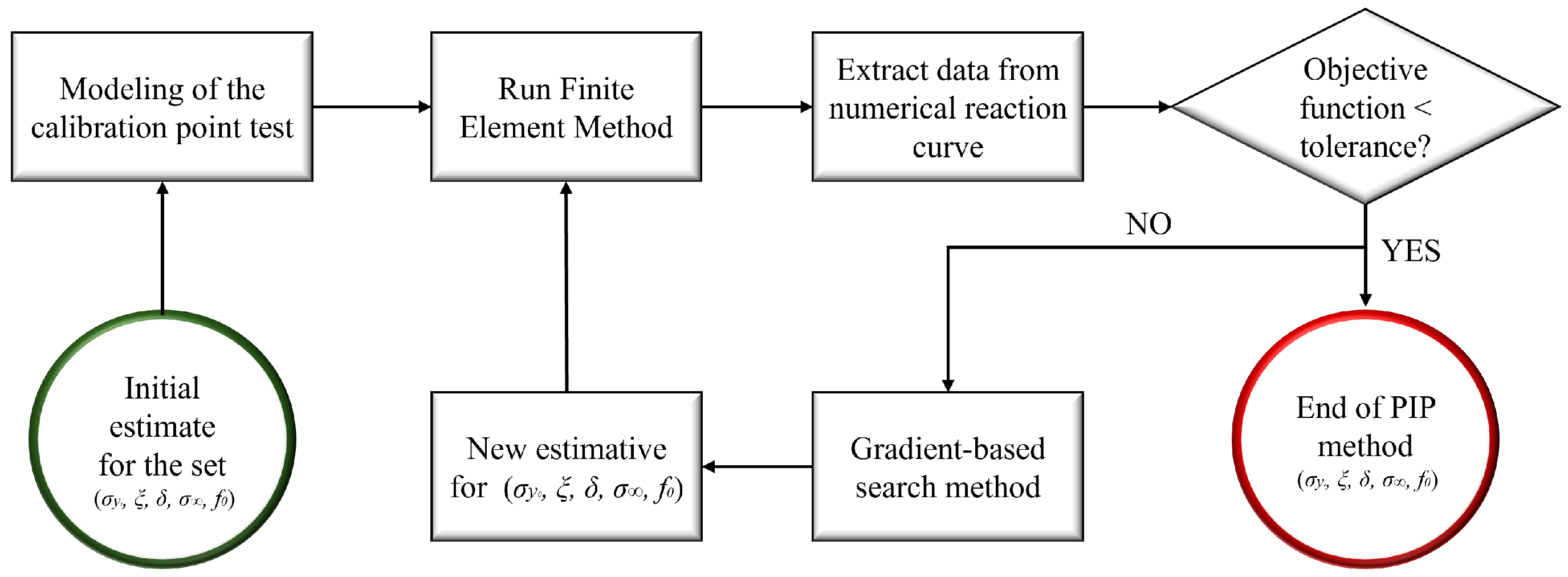
2.2. Parametric Identification Method

The calibration of the parameters of the Kleinermann model, adopted in this work to faithfully reproduce the elasto–plastic behavior of the material, requires a systematic approach that integrates experimental data, microstructural characterization, and numerical optimization. The process focuses on four key parameters of the model: ${\sigma }_{y0}$ (initial yield stress), ${\sigma }_{\infty }$ (saturation stress), $\delta$ (kinematic hardening rate), and $\xi$ (triaxiality sensitivity coefficient).

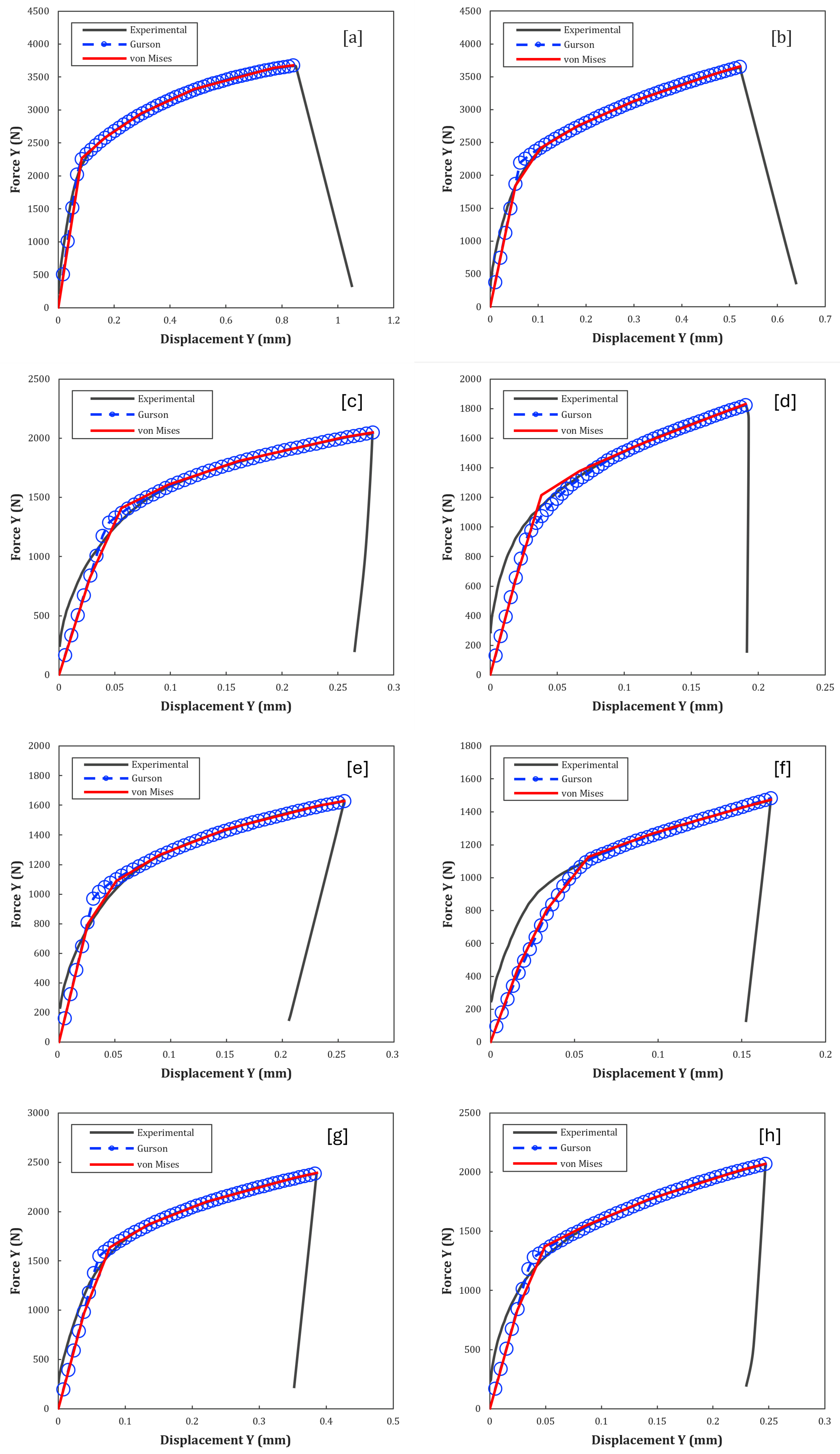
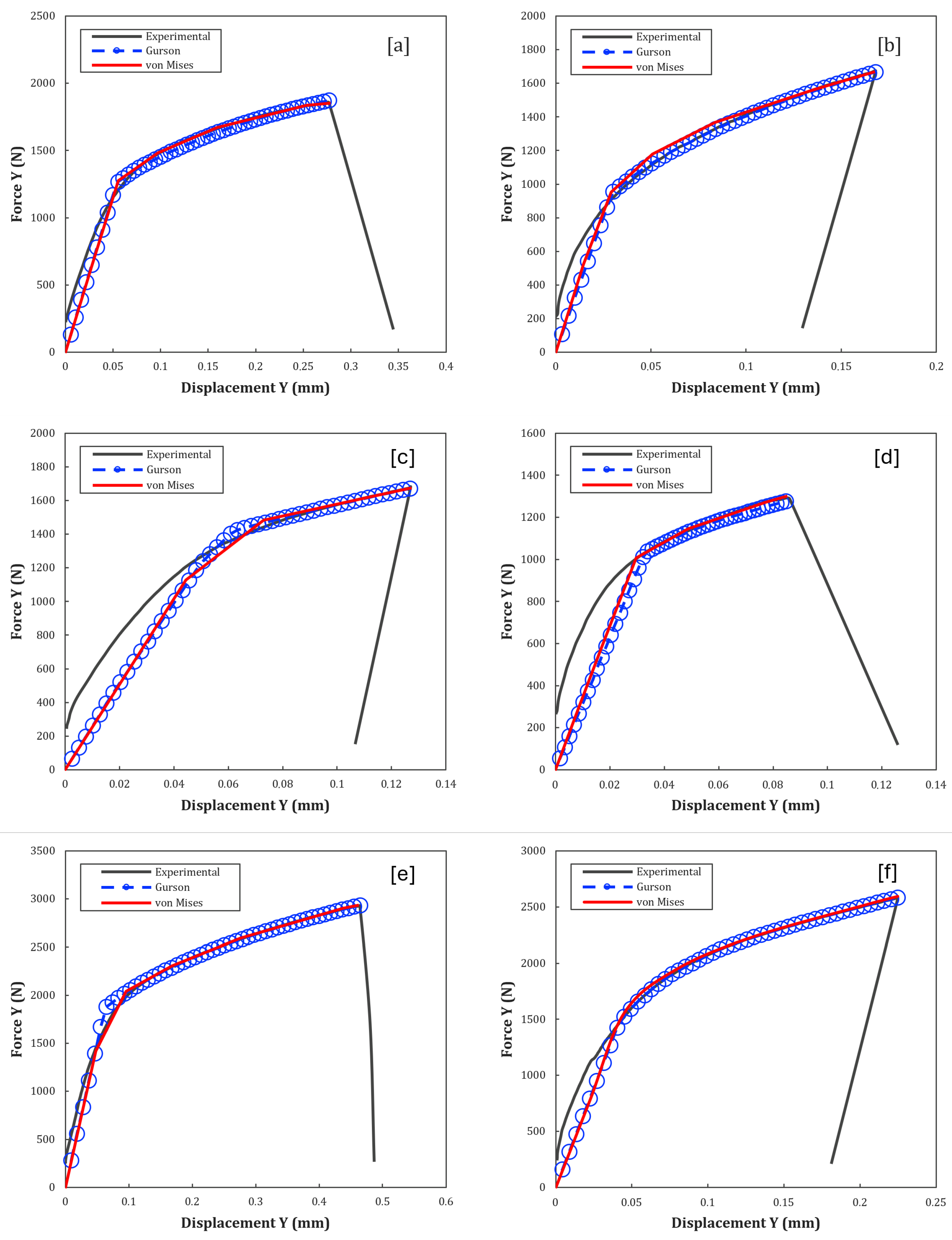
Here, the identification of these parameters begins with the analysis of stress–strain curves obtained from uniaxial tensile tests on specimens manufactured by LPBF, which provide direct information on the yield limit, post-plasticity response, and ductility of the material (see Figure 4).

The initial determination of ${\sigma }_{y0}$ is made directly from the yield point observed experimentally, while ${\sigma }_{\infty }$ is estimated by fitting hardening curves to exponential models. The $\delta$ parameter, which governs the rate of transition between isotropic and kinematic hardening, is derived by analyzing the slope of the stress–strain curve in the plastic phase, using non-linear regression methods. $\xi$, responsible for coupling the influence of the triaxiality of stresses (p) to the evolution of damage, is calibrated by comparing test results under different stress states (e.g., pure traction, shear).

The computational implementation of the Kleinermann [15] model requires solving non-linear constitutive equations, coupled with an implicit return mapping algorithm. This implementation is built on prior knowledge of the elastic deformation (${ϵ}^e$), and the prescribed deformation increment in the known interval $\Delta ϵ$, as well as the set of internal variables at the beginning of the pseudo-time interval [$t_n$, $t_{n+1}$]. These material properties were calibrated using the gradient-based multivariable search method proposed by [16].

With this, the trial state for the start of the iterations is constructed:

$${ϵ}_{n+1}^{e^t}={ϵ}_n^e+\Delta ϵ$$

(16)

$${ϵ}_{n+1}^{p^t}={ϵ}_n^p$$

(17)

$${\sigma }_{n+1}^t={\mathbf{D}}^e:{ϵ}_{n+1}^{e^t}$$

(18)

$${\sigma }_y={\sigma }_y\left({\alpha }_n\right)$$

(19)

$${\alpha }_{n+1}^t={\alpha }_n,$$

(20)

where ${\sigma }_{n+1}^t$ represents the stress tensor of trial state, ${ϵ}_{n+1}^{e^t}$ is the strain tensor of elastic strain of trial state, ${ϵ}_{n+1}^{p^t}$ is the plastic strain of trial state and ${\alpha }_{n+1}^t$ is the internal variable associated with tentative isotropic hardening.

The Newton–Raphson method is used to solve the system of residual equations, where the Jacobian matrix incorporates the partial derivatives with respect to ${\sigma }_{y0}$, ${\sigma }_{\infty }$, $\delta$, and $\xi$. A critical challenge lies in the interdependence between $\delta$ and $\xi$: variations in $\delta$ affect hardening kinetics, while $\xi$ modulates sensitivity to hydrostatic pressure, requiring a delicate balance during optimization.

To validate the robustness of the calibrated parameters, a global sensitivity analysis is carried out, in which each variable is perturbed within physically plausible ranges (e.g., ±10% of ${\sigma }_{\infty }$ or ±15% of $\xi$). This step identifies which parameters have a dominant influence on the model’s predictions: for example, $\xi$ is critical in combined loading (traction-shear), while ${\sigma }_{\infty }$ determines the stability of the response in large deformations.

The final validation is carried out by comparing the predictions of the Kleinermann model with independent experimental results. This approach not only verifies the accuracy of the parameters but also demonstrates the model’s ability to generalize to conditions beyond those used in the calibration. The synergy between experimentation, numerical optimization, and sensitivity analysis consolidates the method as a reliable tool for projects that require precision in predicting damage in materials with a heterogeneous microstructure, typical of additive manufacturing processes.

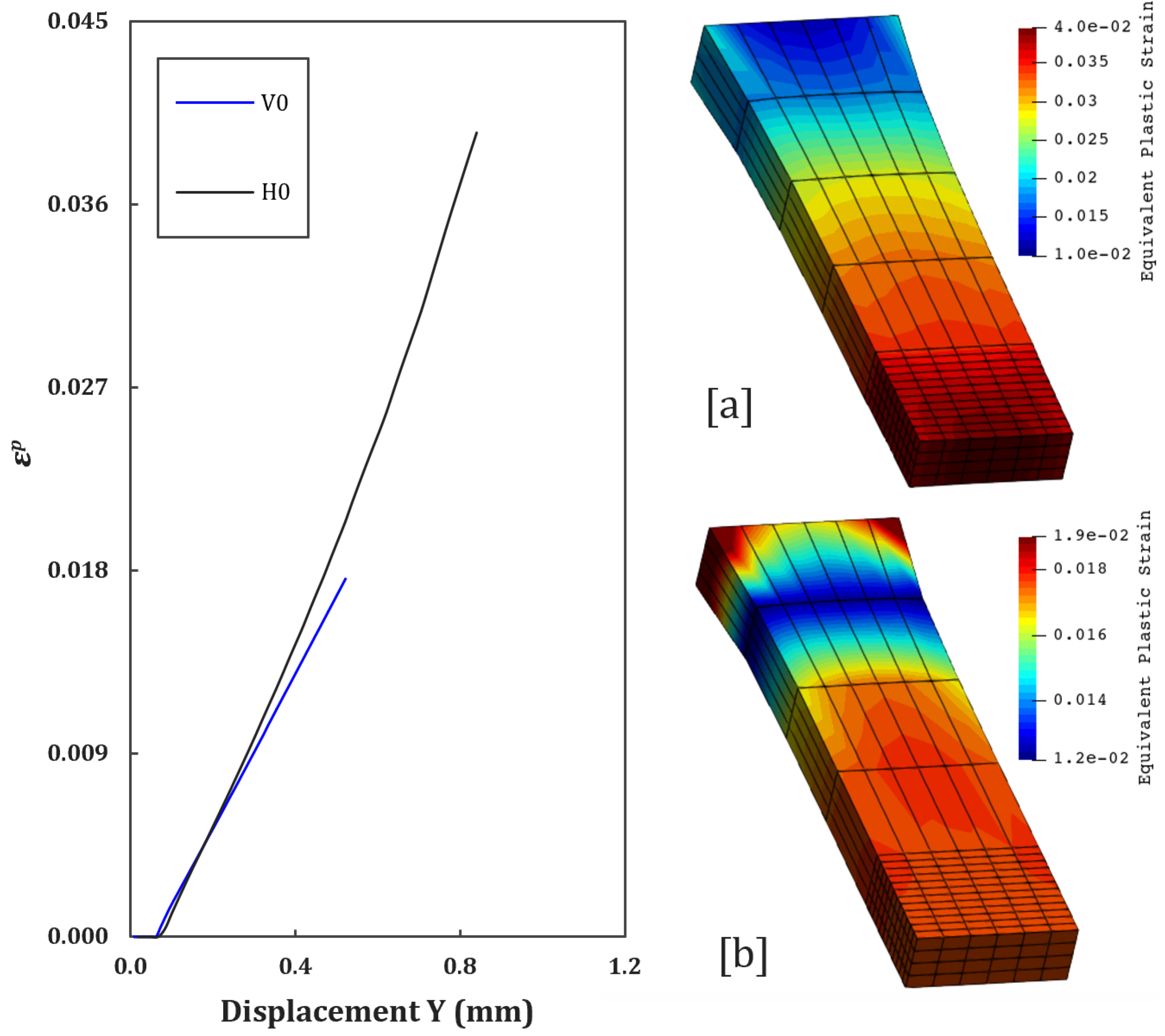
It is important to note that the material’s initial yield strength (${\sigma }_y$) is intrinsically linked to the internal variable (${\alpha }_n$), associated with isotropic hardening. In the von Mises context, the equivalent plastic strain takes on the role of this internal variable, establishing a direct relationship between ${\sigma }_y$ and the history of plastic strain accumulated during loading. In this way, the yield strength is not only used as a criterion that defines the initial strength of the material but also evolves as a function of the progression of plasticity (${\dot{ϵ}}^p$), reflecting the progressive hardening of the microstructure.

In this way, the numerical model developed for Gurson’s mathematical model is summarized as shown in

Table 1. Numerical integration algorithm [17] with Gurson-based model.

(i) Determine the trial state, given a strain increment, $\Delta$$ϵ$:

${ϵ}_{n+1}^{e^t}$=${ϵ}_n^e$+$\Delta$$ϵ$  ${ϵ}_{n+1}^{e^t}$=${ϵ}_n^e$

${\sigma }_{n+1}^t$=${\mathbf{D}}^e$:${ϵ}_{n+1}^{e^t}$  ${\overline{ϵ}}_{n+1}^{p^t}$=${\overline{ϵ}}_n^p$

${\sigma }_y$=${\sigma }_y$${\overline{ϵ}}_n^p$  ${ϵ}_{n+1}^{e^t}$=${ϵ}_n^p$

(ii) Check plastic admissibility:

$\varphi =J_2\left(\mathbf{S}\right)-{\displaystyle \frac{1}{3}}\left[1+f^2-2fcosh\left({\displaystyle \frac{3p}{2{\sigma }_y}}\right)\right]{\sigma }_y^2$

If $\varphi$ ≤ 0, then (elastic step): ${\ast }_{n+1}$ = ${\ast }_{n+1}^t$.

Otherwise, then (plastic step).

(iii) Return mapping: solving the system of non-linear equations (Newton–Raphson), with the following variables: ${\sigma }_{n+1}$, ${ϵ}_n^p$, f, e $\Delta$$\gamma$.

$\left|\begin{array}{cccc}{\displaystyle \frac{\partial R{\sigma }_{n+1}}{\partial {\sigma }_{n+1}}}& {\displaystyle \frac{\partial R{\sigma }_{n+1}}{\partial {\overline{ϵ}}_{n+1}^p}}& {\displaystyle \frac{\partial R{\sigma }_{n+1}}{\partial f}}& {\displaystyle \frac{\partial R{\sigma }_{n+1}}{\partial \Delta \gamma }}\\ {\displaystyle \frac{\partial R{\overline{ϵ}}_{n+1}^p}{\partial {\sigma }_{n+1}}}& {\displaystyle \frac{\partial R{\overline{ϵ}}_{n+1}^p}{\partial {\overline{ϵ}}_{n+1}^p}}& {\displaystyle \frac{\partial R{\overline{ϵ}}_{n+1}^p}{\partial f}}& {\displaystyle \frac{\partial R{\overline{ϵ}}_{n+1}^p}{\partial \Delta \gamma }}\\ {\displaystyle \frac{\partial Rf}{\partial {\sigma }_{n+1}}}& {\displaystyle \frac{\partial Rf}{\partial {\overline{ϵ}}_{n+1}^p}}& {\displaystyle \frac{\partial Rf}{\partial f}}& {\displaystyle \frac{\partial Rf}{\partial \Delta \gamma }}\\ {\displaystyle \frac{\partial R\Delta \gamma }{\partial {\sigma }_{n+1}}}& {\displaystyle \frac{\partial R\Delta \gamma }{\partial {\overline{ϵ}}_{n+1}^p}}& {\displaystyle \frac{\partial R\Delta \gamma }{\partial Rf}}& {\displaystyle \frac{\partial R\Delta \gamma }{\partial \Delta \gamma }}\end{array}\right|·\left|\begin{array}{c}\delta \sigma \\ \delta {\overline{ϵ}}^p\\ \delta f\\ \delta \Delta \gamma \end{array}\right|=-\left|\begin{array}{c}R\sigma \\ R{\overline{ϵ}}^p\\ Rf\\ R\Delta \gamma \end{array}\right|$

(iv) Update other internal variables.

(v) End.

. The Newton–Raphson method is used to solve the non-linear system described in the table above, due to its rapid convergence. The trial state is taken as the initial parameter of the problem.

To solve the non-linear system described in the table above, the Newton–Raphson method is used, one of the advantages of which is its rapid convergence.

Table 2. Return mapping algorithm (Newton–Raphson) for the Gurson-based model.

(i) Given the trial state as initial parameters:

${\sigma }_{n+1}^{\left(0\right)}$=${\sigma }_{n+1}^t$  ${\overline{ϵ}}_{n+1}^{p^t}$=${\overline{ϵ}}_n^p$  $f_{n+1}^{\left(0\right)}$=$f_{n+1}^t$  $\Delta$${\gamma }^{\left(0\right)}$=$\Delta$$\gamma$

(ii) Solve the system of equations for ${\sigma }_{n+1}$, ${\overline{ϵ}}_n^p$, f, e $\Delta$$\gamma$:

$\left|\begin{array}{cccc}{\displaystyle \frac{\partial R{\sigma }_{n+1}}{\partial {\sigma }_{n+1}}}& {\displaystyle \frac{\partial R{\sigma }_{n+1}}{\partial {\overline{ϵ}}_{n+1}^p}}& {\displaystyle \frac{\partial R{\sigma }_{n+1}}{\partial f}}& {\displaystyle \frac{\partial R{\sigma }_{n+1}}{\partial \Delta \gamma }}\\ {\displaystyle \frac{\partial R{\overline{ϵ}}_{n+1}^p}{\partial {\sigma }_{n+1}}}& {\displaystyle \frac{\partial R{\overline{ϵ}}_{n+1}^p}{\partial {\overline{ϵ}}_{n+1}^p}}& {\displaystyle \frac{\partial R{\overline{ϵ}}_{n+1}^p}{\partial f}}& {\displaystyle \frac{\partial R{\overline{ϵ}}_{n+1}^p}{\partial \Delta \gamma }}\\ {\displaystyle \frac{\partial Rf}{\partial {\sigma }_{n+1}}}& {\displaystyle \frac{\partial Rf}{\partial {\overline{ϵ}}_{n+1}^p}}& {\displaystyle \frac{\partial Rf}{\partial f}}& {\displaystyle \frac{\partial Rf}{\partial \Delta \gamma }}\\ {\displaystyle \frac{\partial R\Delta \gamma }{\partial {\sigma }_{n+1}}}& {\displaystyle \frac{\partial R\Delta \gamma }{\partial {\overline{ϵ}}_{n+1}^p}}& {\displaystyle \frac{\partial R\Delta \gamma }{\partial Rf}}& {\displaystyle \frac{\partial R\Delta \gamma }{\partial \Delta \gamma }}\end{array}\right|·\left|\begin{array}{c}\delta \sigma \\ \delta {\overline{ϵ}}^p\\ \delta f\\ \delta \Delta \gamma \end{array}\right|=-\left|\begin{array}{c}R\sigma \\ R{\overline{ϵ}}^p\\ Rf\\ R\Delta \gamma \end{array}\right|$

(iii) Calculate:

${\sigma }_{n+1}^{\left(k+1\right)}$=${\sigma }_{n+1}^{\left(k\right)}$+$\delta {\sigma }_{n+1}^{\left(k+1\right)}$   ${\overline{ϵ}}_{n+1}^{p^{\left(k+1\right)}}$=${\overline{ϵ}}_{n+1}^{p^{\left(k\right)}}$+ $\delta$${\overline{ϵ}}_{n+1}^{p^{\left(k+1\right)}}$

$f_{n+1}^{\left(k+1\right)}$=$f_{n+1}^{\left(k\right)}$+$\delta f_{n+1}^{\left(k+1\right)}$   $\Delta$${\gamma }^{\left(k+1\right)}$=$\Delta$${\gamma }^{\left(k\right)}$+$\delta$$\Delta$${\gamma }^{\left(k+1\right)}$

(iv) Verify the convergence:

${\varphi }^{k+1}=J_2\left(\mathbf{S}\right)-{\displaystyle \frac{1}{3}}\left[1+{\left(f_{n+1}^{k+1}\right)}^2-2f_{n+1}^{k+1}cosh\left({\displaystyle \frac{3p_{n+1}}{2{\sigma }_y}}\right)\right]{\sigma }_y^2$

$\mathit{erro}={\displaystyle \frac{{\varphi }^{k+1}}{\frac{1}{3}\left[1+{\left(f_{n+1}^{k+1}\right)}^2-2f_{n+1}^{k+1}cosh\left(\frac{3p_{n+1}}{2{\sigma }_y}\right)\right]{\sigma }_y^2}}\le \mathit{tolerance}$

(v) End.

summarizes the application of the Newton–Raphson method to solve the linear system mentioned above, where the trial state is taken as the initial parameter of the problem.

The residual matrix encapsulates all the non-linear equations governing the behavior of the material in the elasto–plastic regime. Each residue to the left of the equation measures the deviation between the current state of the variables and the physical equilibrium conditions (such as the evolution of porosity). One of the key points for this approach is the definition of the simulation’s stopping criterion, also known as critical damage [18]. During each Newton–Raphson iteration, the residuals are calculated, and their partial derivatives are used to incrementally correct the variables $({\sigma }_{n+1},{\dot{ϵ}}_{n+1}^p,f_{n+1},\Delta \gamma )$ until the residuals are reduced below a predefined tolerance (e.g., ${10}^{-6}$).

The method is therefore essential to ensure that the Gurson model accurately reproduces phenomena such as the expansion of voids under triaxial tension, the progressive reduction in stiffness due to increased porosity, and the transition between elastic and plastic regimes.

2.3. Method for Assessing Adhesion Between Models and Tensile Test

To assess the adherence between a curve obtained experimentally and another via computer simulation (force versus displacement, in this case), it is necessary to compare them quantitatively, using statistical metrics that guide the degree of similarity or difference between them. There are various approaches and statistical parameters that can be used for this, depending on the context and the desired precision: Root Mean Square Error, Coefficient of Determination ($R^2$), Mean Relative Error, Visual Comparison, etc.

As it provides a percentage metric, useful for comparing curves that have different scales, the Mean Relative Error (MRE) evaluation technique is the most effective for this work. The statistical consensus is that an average relative error below 10% is considered good, given that this depends on the experimental context.

$$ERM={\displaystyle \frac{1}{n}}\sum _{i=1}^n{\displaystyle \frac{|y_{\exp ,i}-y_{\mathrm{sim},i}|}{|y_{\exp ,i}|}}$$

(21)

where $y_{\mathrm{ref},i}$ is the strength of the reference curve (experimental), $y_{\mathrm{yes},i}$ is the interpolated strength of the evaluated curve (simulation by the von Mises or Gurson model), and n is the number of points on the curve.

3. Methodology

This chapter details the strategy adopted to investigate the relationship between porosity and mechanical properties in materials manufactured by AM, with emphasis on the implementation of the Gurson model for damage prediction. The methodology is divided into three main axes:

• Fabrication and experimental characterization of specimens;
• Development of the numerical model based on the Gurson criterion;
• Validation of the results with the Gurson model via comparison with experimental data and simulations with the von Mises model.

The data collected was analyzed using academic computing platforms, enabling the parameters of each model to be calibrated. In addition, the initial porosity and the limit porosity for the Gurson model were determined, being 0.001 and 1.0, respectively.

In the parametric identification stage, an iterative procedure based on the force versus displacement curve for the objective function was adopted, using the least squares method. A gradient-oriented method was used for the search strategy, while the problem was solved numerically using finite elements.

At the end, the experimental results are compared with the numerical results of each simulation, in order to highlight the influence of the degree of porosity (composed of the distance between voids and their diameters) and the mechanical strength of each specimen, observing the impact of the variation in the density of the piece on the level of plastic strain and the fracture of the material.

4. Specimens Manufacturing

Flat specimens were prepared on the basis of [19], designed to allow the variation of voids in the notch region of the specimen. All the specimens had the same geometric dimensions, with a useful notch length of 13 mm. Fourteen AlSi10Mg specimens were manufactured using the LPBF technique, with strict control of process parameters:

• Printing direction: Seven specimens with vertical withdrawal (y)—named V0, V2, V3, V5, V6, V7, and V8—and seven specimens with horizontal withdrawal (x)—named H0, H2, H3, H5, H6, H7, and H8—to assess mechanical anisotropy.

It is important to mention that specimens V1, V4, H1, and H4 were not considered for this work. Figure 5 shows how these specimens are removed, taking into account the printing direction adopted as a strategy.

To introduce controlled variability in porosity, the specimens were designed with different volume fractions of voids, ranging from configurations with no controlled porosity (H0 and V0) to configurations with low theoretical density (e.g., H7/V7 and H8/V8). Figure 6 shows the specimens produced via LPBF, accompanied by their respective void distributions. This figure highlights the spatial arrangement of the voids, with sizes varying between 0.2 mm and 0.6 mm and spacings between 0.3 mm and 1.5 mm, as detailed in

Table 3. Identification of the specimen according to its printing direction, with each void dimension.

Printing Direction	Specimen ID	Void Diameter d [mm]	Distance Between Voids in x [mm]	Distance Between Voids in y [mm]	Theoretical Density [%]
(V) Vertical	0	0	0	0	100
(H) Horizontal		0	0	0	100
(V) Vertical	2	0.4	0.8	0.8	80.37
(H) Horizontal		0.4	0.8	0.8	80.37
(V) Vertical	3	0.6	1.2	1.2	80.37
(H) Horizontal		0.6	1.2	1.2	80.37
(V) Vertical	5	0.4	1	1	87.43
(H) Horizontal		0.4	1	1	87.43
(V) Vertical	6	0.6	1.5	1.5	87.43
(H) Horizontal		0.6	1.5	1.5	87.43
(V) Vertical	7	0.2	0.3	0.5	79.06
(H) Horizontal		0.2	0.3	0.5	79.06
(V) Vertical	8	0.2	0.5	0.5	87.43
(H) Horizontal		0.2	0.5	0.5	87.43

.

The introduction of controlled voids was achieved by adjusting the parameters of the LPBF process, such as laser power, scanning speed, and layer thickness, allowing the formation of pores with specific dimensions and distributions. These adjustments were carefully calibrated to ensure that the voids were representative of the typical defects found in AM-manufactured components, such as gas pores or a lack of fusion, as illustrated previosly in Figure 3.

The specimens without intentional voids (theoretical density of 100%) served as a reference for comparing the mechanical degradation caused by controlled porosity.

When simulating the plane state of stress, symmetry was taken into account in the middle section of the specimen, with this being the place of interest where plastic strains were observed experimentally using a Strain Gauge. The integration of controlled manufacturing, characterization, and mechanical testing allowed for a robust analysis of the influence of porosity on the material’s response, providing a solid basis for the numerical–experimental comparisons presented in this work.

Finite Element Geometry and Mesh

The specimens used to test the robustness of the proposed numerical models were modeled with the mechanical properties of AlSi10Mg under classic flat geometry (rectangular section). Monotonic loading was applied until total failure of the specimen, and in the simulation, the loading boundary condition was given by the prescribed fracture displacement obtained from the experimental test.

Defining the geometry of the specimens and generating the finite element mesh are fundamental steps in ensuring the representativeness of the numerical simulations carried out using the Gurson-based model. The specimens were designed based on the dimensional specifications presented in

Table 4. Size of the section of interest for the numerical simulations, as shown in Figure 7.

Specimen	a [mm]	b [mm]	c [mm]
H0	5.503	13	1.970
H2	5.515	13	1.974
H3	5.502	13	1.950
H5	5.512	13	1.984
H6	5.512	13	1.975
H7	5.498	13	1.939
H8	5.495	13	1.990
V0	5.500	13	2.032
V2	5.494	13	2.000
V3	5.495	13	1.985
V5	5.488	13	1.988
V6	5.502	13	1.985
V7	5.499	13	2.030
V8	5.496	13	2.047

, which details the dimensions of the section of interest used in the simulations. The geometry was designed to replicate the experimental conditions of uniaxial traction, allowing analysis of the influence of porosity and printing direction (horizontal and vertical) on the mechanical response of the material manufactured via LPBF.

Figure 7 illustrates the section of interest of the specimens, highlighting the spatial distribution of the controlled voids. This figure is crucial for visualizing the location and size of the pores, which were intentionally introduced to simulate typical additive manufacturing defects, such as gas pores or a lack of fusion, as discussed in the theoretical basis topic [20]. CT analysis made it possible to validate the accuracy of the manufactured geometry, confirming that the voids corresponded to the designed dimensions.

The finite element mesh was generated using 8-node hexahedral elements (HEXA8), chosen because of their ability to accurately model the three-dimensional behavior of the material under load. The mesh was structured to ensure sufficient density in the regions near the voids, where the concentration of stresses is most pronounced, as can be seen in Figure 6. This figure, which shows the specimens with their respective void distributions, was used as a reference to define the discretization of the mesh, ensuring that the pores were adequately represented in the numerical model. The density of the mesh was refined in the vicinity of the voids, with an average element size of 0.1 mm in critical regions, while 0.5 mm elements were used in areas less susceptible to plastic strain. This refinement strategy was essential to capture the stress and strain gradients associated with damage evolution, as described by the Gurson model.

The mesh was generated using the pre-processing software, which enabled the creation of a structured mesh with 595 nodes. This number of nodes was validated to ensure convergence of the numerical simulations, with preliminary tests indicating that a further increase in mesh density (>600 nodes) did not result in significant improvements in the accuracy of the results but increased the computational cost. The boundary conditions were defined to replicate the uniaxial tensile test, with displacement imposed at the upper end of the specimen and full restraint at the lower end, ensuring that the loading was consistent with the experimental tests.

The geometric data and the finite element mesh were exported to an academic framework called HYPLAS [17], which was used for the numerical simulations based on the Gurson model. The integration of the geometry, mesh, and manufacturing process parameters ensured that the simulations faithfully reflected the experimental conditions. The analysis of Figure 5, Figure 6, and Figure 7 was essential for correlating the physical geometry of the specimens with the experimental results and numerical models, allowing for an accurate assessment of the influence of porosity and anisotropy on the material’s mechanical response.

5. Results and Discussion

5.1. Experimental Results

Using Table 3, which shows the theoretical density of each specimen as a function of the size of the void inserted, as well as the distance between each void in the x and y directions, it is possible to illustrate the relationship between force and displacement in the experimental tests for the specimens manufactured via AM (see Figure 8). Comparative analysis of the curves allows us to identify critical patterns associated with the influence of the theoretical density, the size of the voids, and the spacing between them on the mechanical behavior of the material.

5.1.1. Specimens Without Controlled Porosity (H0 and V0)

The H0 and V0 curves, corresponding to specimens with a theoretical density of 100%, show the highest mechanical strengths of all the configurations tested. The initial elastic phase curve is marked by high rigidity, reflecting the structural integrity of the metal matrix without defects. The yield point is reached at significantly close force values for both printing directions, which allows us to conclude that the printing direction did not affect the material’s behavior up to this point. Fracture occurs after a displacement of 0.8 mm for the horizontal printing direction, and just after 0.5 mm for the specimens made vertically via AM.

When compared to H0, the premature fracture observed in the V0 specimen critical displacement of 0.6 mm, versus 1 mm in H0 reveals an expected anisotropic mechanical behavior. This difference is directly associated with the orientation of the layers during printing and the resulting microstructural characteristics. This observed anisotropy reinforces the need to orient critical parts during printing so that the layers are parallel to the main loading directions, maximizing strength and ductility.

The results from [21], in metal additive manufacturing, report that tensile strength in the vertical direction can be 10–30% lower than in the horizontal direction, depending on the material and the process. The reduction in ductility in V0 is also in line with observations that interfaces between layers act as preferential sites for crack initiation, i.e., a lower preferential alignment of grains with the loading direction perpendicular to the printing layers to the vertical. This results in a less cohesive microstructure, with less capacity to redistribute stresses efficiently, when compared to the H direction (parallel to loading).

5.1.2. Effect of Theoretical Density Reduction

The effect of theoretical density reduction is as follows:

• Configuration H2 and V2 (80.37% theoretical density, with 0.4 mm voids and 0.8 mm spacing between voids): Reducing the density to 80.37% results in a decrease in stiffness and maximum supported strength, compared to bodies with an apparent density of 100%. The presence of larger (0.4 mm) and more closely spaced voids acts as stress concentrators, accelerating crack nucleation and reducing ductility. The plastic curve is less pronounced, with fracture occurring at displacements close to 0.2 mm.
• Configuration H3 and V3 (80.37% theoretical density, with 0.6 mm voids and 1.2 mm spacing between voids): Despite the same theoretical density as H2 and V2, the increase in void diameter and spacing results in a further reduction in strength. The larger size of the voids amplifies the concentration of local stresses, while the wider spacing allows for greater plastic strain before the defects coalesce. This explains the greater deformation to fracture compared to H2 and V2, but assuming a lower maximum strength.
• Configuration H5 and V5, and H6 and V6 (87.43% theoretical density): Specimens with a higher theoretical density show intermediate performance between H0 and V0, and H2 and V2. In H5 and V5 (0.4 mm voids and 1 mm spacing), the lower void density allows for greater resistance than H2 and V2 but less than H0 and V0. In H6 and V6 (0.6 mm voids and 1.5 mm spacing), the greater distance between voids reduces the interaction between defects, delaying fracture and increasing relative ductility, although the maximum strength remains lower than that of H5 and V5.

5.1.3. Configurations with Low Theoretical Density

The H7 and V7 curves (79.06% density) stand out for their drastic reduction in strength and stiffness. The high density of small voids (0.2 mm) creates a network of distributed stress concentrators, facilitating early crack nucleation and limiting plastic strain capacity. Fracture occurs abruptly, characterizing brittle behavior, contrasting with the ductility observed in less porous specimens.

5.1.4. Anisotropy Induced by the Printing Direction

A comparison between horizontally (H) and vertically (V) manufactured specimens reveals significant differences in mechanical response. In general, the H curves exhibit greater initial stiffness and maximum strength than their V counterparts, possibly due to the orientation of the layers. In the horizontal direction, the layers are deposited parallel to the loading, optimizing load transfer. In the vertical direction, the interfaces between layers act as planes of weakness with lower strength.

5.1.5. Fracture Mechanisms and Coalescence of Voids

In all configurations, post-flow non-linearity in the curves is associated with the growth and coalescence of voids. In bodies with a high density of defects (e.g., H7 and V7), coalescence occurs early, limiting plastic strain. In contrast, in bodies with a lower density of voids (e.g., H6 and V6), the plastic phase is more prolonged, indicating that the metal matrix is able to redistribute stresses before final failure.

The experimental results validate the importance of precise porosity control throughout the AM process. The theoretical and geometric density of the voids (diameter and spacing) are critical parameters for balancing the strength and lightness of the manufactured part. For example, configurations such as H5 and V5 offer an acceptable compromise between strength loss (15–20% compared to H0 and V0) and weight reduction, while configurations such as H7 and V7 are only suitable for non-structural applications.

5.2. Numerical Results

5.2.1. Comparison Between von Mises and Gurson

The comparison between the predictions of the constitutive models (von Mises and Gurson) and the experimental data reveals critical nuances about the ability of each theory to capture deformation and damage mechanisms in porous materials. In this chapter, each configuration is analyzed with an emphasis on the physical foundations that explain the differences in fitting curves between models and tensile tests (see Figure 9 and Figure 10).

Table 5. Comparison of relative error between the models and the experimental test curve.

Specimen	Mean Relative Error	Gurson
	von Mises
V0	6.48%	6.17%
H0	6.04%	4.79%
V2	11.33%	10.18%
H2	10.20%	9.72%
V3	16.98%	16.41%
H3	8.44%	7.59%
V5	8.22%	7.89%
H5	7.77%	7.42%
V6	9.38%	9.15%
H6	9.79%	9.50%
V7	21.35%	19.06%
H7	19.65%	19.60%
V8	9.16%	8.71%
H8	6.48%	6.06%

shows that 7 of the 28 simulations had a statistically weak fitting. The poor quality of the experimental curves obtained in the V3, V7, and H7 tests proved to be a determining factor for this weak adherence in both models (von Mises and Gurson), as explained previously. In the case of V2, the low fitting is clearly attributed to the abrupt transition step between the elastic and plastic phases of the curve. This type of behavior in simulations is quite common when the numerical model tries to have good adherence in both parts of the curve, causing this transition between them to be forced.

For all the curves, the Gurson model had a lower ERM, although in some cases slightly lower, than the von Mises model. This analysis is important because the difference in fitting between the models tends to be small in percentage terms but still extremely important for the evolution of the material’s behavior under loading conditions.

5.2.2. Comparison of Constitutive Model Parameter Results

Table 6. Result of the material hardening curve parameters for vertical printing specimens after implementation of the search method based on the Gurson model.

Vertical Printing
Specimen	V0	V2	V3	V5	V6	V7	V8
Density	100%	80.37%	80.37%	87.43%	87.43%	79.06%	87.43%
E [MPa]	69,000	68,000	70,000	70,000	62,000	70,000
${\mathit{\sigma }}_{\mathit{y}\mathbf{0}}$ [MPa]	270.50	147.01	152.20	121.38	153.63	100.21	150.90
$\mathit{\xi }$ [MPa]	4726.50	9143.35	1457.03	607.77	2693.58	1639.18	9482.02
${\mathit{\sigma }}_{\infty }$ [MPa]	405.90	196.12	172.60	225.50	224.67	131.51	201.80
$\mathit{\delta }$	96.90	25.32	64.20	119.63	184.97	455.16	1102.80
${\mathit{f}}_{\mathbf{0}}$	0.252	0.255	0.172	0.093	0.332	0.064	0.113

and

Table 7. Result of the material hardening curve parameters for horizontal printing specimens after implementation of the search method based on the Gurson model.

Horizontal Printing
Specimen	H0	H2	H3	H5	H6	H7	H8
Density	100%	80.37%	80.37%	87.43%	87.43%	79.06%	87.43%
E [MPa]	81,000	80,000	75,500	68,000	65,000	62,000	70,000
${\mathit{\sigma }}_{\mathit{y}\mathbf{0}}$ [MPa]	214.30	121.20	114.30	158.30	181.20	105.90	193.70
$\mathit{\xi }$ [MPa]	712.50	3548.30	3664.50	3766.90	2114.10	4861.56	3783.40
${\mathit{\sigma }}_{\infty }$ [MPa]	352.40	159.70	159.50	198.60	277.50	133.90	251.02
$\mathit{\delta }$	67.90	423.90	319.10	262.40	178.60	46.56	159.02
${\mathit{f}}_{\mathbf{0}}$	0.038	0.028	0.077	0.023	0.171	0.056	0.103

provide a critical analysis of the behavior of the material in the different configurations, shown here in terms of the diameter of the voids, the direction of printing, and the distance between voids (the density of the specimen being a consequence of the changes in these parameters).

All the specimens, when compared to their counterparts in the other printing direction, showed similar E and ${\sigma }_{y_0}$ parameters (i.e., when comparing V0 with H0, V2 with H2, and so on). This indicates that the elastic behavior is independent of the AM printing direction.

To continue discussing the results in the table, it should be remembered that $\xi$ is an indicator of the material’s thermomechanical history. It can be seen that there is a variation (and inversion) of $\xi$ with the AM manufacturing direction. In other words, the interaction between the process parameters (such as printing speed and power) and the hardening mechanisms for each configuration of voids affects the microstructure of the material in a complex way, impacting the rate of isotropic hardening.

All the specimens, when compared to their counterpart in the other printing direction, showed similar e ${\sigma }_{\infty }$ parameters (i.e., when comparing V0 with H0, V2 with H2, and so on). This indicates that the printing direction does not alter the quantification of the maximum isotropic hardening that the material can achieve after significant plastic strain. Furthermore, it is extremely important to infer that the low values of ${\sigma }_{\infty }$ found, and the fact that they are, in all cases, close to ${\sigma }_{y_0}$ indicates that the material does not harden significantly when exposed to loading. Again, this analysis for this parameter applies to all the specimens, including those with a theoretical density of 100% (V0 and H0). However, it can be seen that of all the specimens, these have the greatest capacity to withstand stresses after large deformations.

It can also be seen that the anisotropy induced by the manufacturing direction affects the $\delta$ parameter critically. The $\delta$ results for V0 and H0 indicate this, as for these cases, the result is relatively close. However, there are a number of $\delta$ variations that must be analyzed when porosity is induced in the material, at different distances and diameters, for the different AM manufacturing directions. The higher $\delta$ values in H2 and H3 indicate that the printing direction (in relation to loading) generates faster kinematic hardening, when compared to their corresponding V2 and V3, a behavior typical of materials with a high density of disagreements. However, looking at the results for V7 and H7, the evolution of kinematic hardening is greater for the specimen obtained vertically, which is the opposite of the intuitive result for H2 and H3. This suggests that the evolution of the induced anisotropy may be the opposite of what is expected in cases of low specimen density. In other words, in addition to the printing direction, the low density $\approx 79$% causes the model to show significant variations for materials with brittle behavior, which also justifies the addition of the Gurson model to this constitutive modeling. Therefore, a better discussion of this behavior can be made when analyzing $f_0$.

Analyzing the porosity parameter for V0 and H0, despite both having a theoretical density of 100% (theoretically without porosity), the $f_0$ values are not zero, indicating the presence of residual porosity inherent in the additive manufacturing process. The highest $f_0$ is in V0 (0.252), suggesting that vertical printing can introduce more defects (such as pores or microcracks) compared to horizontal printing (0.039), due to the orientation of the layers, which in the vertical direction can lead to greater coalescence of defects that are introduced inherent to the manufacturing process, unlike the defects controlled in subsequent specimens.

In general, the vertical specimens (V0, V3, V5, V6) have higher $f_0$ than the horizontal ones, except in specific cases explained by their low densities, which compromise the isotropic hardening of the material (V7 and H7). V8 and H8 have practically the same value of $f_0$ $\approx 0.1$, but V8’s $f_0$ is still higher than H8’s. The size and spacing of the voids affect the interaction between them during deformation. Larger and more widely spaced voids (as in V6 and H6) can amplify the local effect of stress concentration, especially in the vertical direction, where the microstructure is more susceptible to defects.

Larger voids (0.6 mm in V3, H3, V6, H6) tend to increase $f_0$, as they cause greater stress concentration and facilitate the nucleation and growth of voids during deformation. In addition, the reduced theoretical density (80.37% or 79.06%) reflects greater initial porosity, which adds to the added voids, influencing $f_0$.

In short, in the vertical direction, the interfaces between layers are aligned with the direction of traction, which can amplify defects such as a lack of fusion or porosity, increasing $f_0$. Beyond the printing direction, the larger the void size, and the less spacing between them, the more favorable to damage. Although the stress concentration factor is constant, the cross-sectional area will be reduced in this scenario, increasing the maximum local stress.

5.3. Damage Evolution

5.3.1. Evolution of Accumulated Plastic Deformation

With the results, it is possible to describe the evolution of the plastic strain in the specimens manufactured via AM, simulated numerically using the Gurson model implemented in HYPLAS (see Figure 11, Figure 12, Figure 13, Figure 14, Figure 15, Figure 16 and Figure 17). These curves allow us to evaluate how controlled porosity and printing direction influence material degradation under mechanical loading.

The H0 and V0 curves in Figure 11, corresponding to specimens with a theoretical density of 100%, show a gradual evolution of plastic strain. It is noticeable that, in all cases, the evolution of plastic strain is slight for the specimens removed in vertical printing (V), when compared to the more prolonged H plastic strain evolution curves (understood as less severe), corroborating the values obtained for $f_0$, where they will always be greater than the accumulated plastic strain, causing the material to exhibit embrittled behavior. The smooth, continuous curve indicates that the material supports homogeneous plastic strain before the coalescence of intrinsic micro voids, which is also in line with the experimental results. The difference between H0 and V0 in the final phase (more accelerated damage in V0) reinforces the microstructural anisotropy, already discussed previously, where the vertical direction introduces more vulnerable interfaces.

From V2 and H2 to V8 and H8 curves (see Figure 12, Figure 13, Figure 14, Figure 15, Figure 16 and Figure 17), it is possible to observe the effect of the introduction of controlled porosity on the evolution of plastic deformation, as presented in

Table 8. Equivalent plastic strain in the fracture.

Specimen	${\mathit{ϵ}}^{\mathit{p}}$
V0	0.017
H0	0.038
V2	0.005
H2	0.011
V3	0.005
H3	0.009
V5	0.009
H5	0.013
V6	0.002
H6	0.008
V7	0.002
H7	0.003
V8	0.006
H8	0.017

).

For the H2 and V2 configurations, the reduction in density to 80.37% anticipates damage initiation. The proximity between voids (0.8 mm) facilitates the interaction of stresses, reducing the material’s ability to redistribute plastic energy. Regarding H3 and V3, although the density is the same as for H2 and V2, the larger diameter of the voids (0.6 mm) amplifies the concentration of local stresses, resulting in earlier damage initiation in the vertically obtained specimen. However, the larger spacing between voids in H3 and V3 (1.2 mm) delays coalescence, generating a less abrupt curve than H2 and V2.

Among the specimens with imposed defects, H5 and V5 have the highest theoretical density (87.43%), delaying damage initiation.For example, H6 and V6 have wide spacing between voids (1.5 mm), allowing greater deformation before coalescence, resulting in a smoother damage curve, with fracture predicted for larger displacements.

For H7 and V7, the high density of small, close voids leads to catastrophic degradation. Damage starts almost immediately, with accelerated growth due to the interaction between multiple stress concentrators. The curve is close to brittle behavior, validating experimental observations of premature fracture.

Finally, H8 and V8 show intermediate degradation. Damage starts early, but the growth phase is moderate, suggesting that smaller voids, even in close proximity, have less impact than large voids.

The vertical curves (from 0 to 8) show a greater sensitivity to deformation than the horizontal ones, for all configurations.

• V2 vs. H2: The V2 curve reaches critical damage at ≈0.18 mm, while H2 requires ≈0.3 mm of displacement.
• V7 vs. H7: Fracture occurs at ≈0.12 mm for V7, against ≈0.18 mm for H7.

This difference is attributed to the orientation of the layers in additive manufacturing. As shown in the experimental results, in the vertical direction (V), the interfaces between layers act as barriers to the propagation of plastic strain, concentrating stresses, and accelerating the coalescence of the voids. In the horizontal direction (H), the alignment of the layers with the loading favors the redistribution of stresses, prolonging the life of the material.

5.3.2. Initial Porosity Evolution

As observed, the simulations qualitatively reproduce the trends observed experimentally:

• Positive correlation between porosity and degradation: Configurations with lower theoretical density (e.g., V7/H7) show accelerated damage, as in the experimental force–displacement curves.
• Effect of void size and spacing: Larger voids (0.6 mm) anticipate fracture, while wide spacings (1.5 mm) delay coalescence, a pattern observed both numerically and experimentally.

Figure 18 and Figure 19 show that the configurations with the highest initial porosity (H6, H8, and V6, V8) reach the point of porosity acceleration at smaller displacements than the configurations with the lowest porosity (H0, H5, and V0, V5). This is to be expected, as a higher void volume fraction ($f_0$) reduces the effective load-bearing area, anticipating damage initiation.

However, a more detailed analysis reveals that the spacing between voids also plays a crucial role. For example, in configurations H7 and V7, and H8 and V8, which have larger voids (0.6 mm) and smaller spacings (1.0 mm), coalescence occurs earlier compared to H5 and V5, which have 0.5 mm voids and 1.5 mm spacings. This effect is consistent with the [12] model, where the proximity between voids facilitates their interaction and coalescence. Although there is an influence of triaxial stresses on damage evolution, the presence of voids locally induces multiaxial stress states, especially in configurations with larger voids.

Another important observation is the possible nucleation of new voids during loading, especially in configurations with lower initial porosity (H0 and V0). If the porosity increases faster than expected just by the growth of pre-existing voids, this may indicate the nucleation of new voids, a phenomenon that the original Gurson model does not explicitly consider.

6. Conclusions

This work investigated the influence of initial porosity and its evolution in metallic materials manufactured by additive manufacturing (AM), with an emphasis on applying the Gurson model to predict the mechanical behavior of specimens produced via Laser Powder Bed Fusion (LPBF). Through an integrated approach that combined experimental tests, numerical simulations, and parametric identification methods, it was possible to achieve the proposed objectives, providing significant contributions to the understanding of the relationship between porosity, anisotropy, and mechanical properties in metallic materials.

The experimental results showed that the printing direction (horizontal and vertical) has a significant impact on the mechanical behavior of the specimens. Vertically deposited specimens (V0–V8) fractured at smaller displacements compared to horizontally deposited specimens (H0–H8), indicating that the anisotropy induced by the AM process directly influences fracture resistance. This difference was attributed to the interfaces between layers in the vertical direction, which act as stress concentrators, accelerating the coalescence of voids, as observed in the force–displacement curves.

Numerical simulations based on the Gurson model, compared to the von Mises model, showed greater accuracy in predicting the evolution of damage and fracture in porous materials. Incorporating the volume fraction of voids (f) and hydrostatic pressure (p) into the flow function made it possible to capture the effects of porosity on reducing stiffness and anticipating fracture, especially in configurations with low theoretical density (e.g., H7/V7). The validation of the numerical results with the experimental ones confirmed the representativeness of the Gurson model for materials manufactured by AM, with consistent correlations between the numerical and experimental curves.

The implementation of the parametric identification method (PIP) for the Kleinermann parameters (${\sigma }_{y0}$, ${\sigma }_{\infty }$, $\delta$, $\xi$) was successful, allowing accurate calibration of the constitutive model. Sensitivity analysis revealed that the parameter $\xi$, related to the triaxiality of stresses, exerts a dominant influence in predicting behavior under combined loading, while ${\sigma }_{\infty }$ is critical for large deformations. These results reinforce the robustness of the model for applications in materials with a heterogeneous microstructure.

In addition, analysis of the evolution of porosity highlighted that larger voids and reduced spacing accelerate coalescence, reducing the ductility of the material. This observation is particularly relevant for the design of components manufactured by AM, where porosity control can optimize the relationship between weight reduction and mechanical performance.

In summary, this work has shown that the Gurson model, combined with a robust experimental and numerical methodology, is an effective tool for predicting the behavior of porous metallic materials manufactured by AM. The validation of the proposed methodology establishes a reliable standard for evaluating the impact of printing direction and density on mechanical strength, meeting the specific objectives outlined.

7. Future Work

For future work, the author recommends investigating different metal alloys, such as stainless steels or nickel superalloys, to evaluate the generalization of the Gurson model in other materials manufactured by AM. The use of techniques for crystallographic evaluation of the material is necessary to understand how the grain contours are affected by the AM parameters, and how these crystallographic configurations affect the material’s isotropic hardening parameters (as in the $\xi$ analysis carried out in Section 5.2.2). Furthermore, the use of the Gurson–Tvergaard–Needleman (GTN) model incorporates nucleation terms, and the data in Figure 18 and Figure 19 can be used to calibrate these parameters in future studies. Finally, extending the model to dynamic or cyclic loading could expand its applicability to fatigue conditions [22], which are also relevant to various applications.