Article

MNATS: A Multi-Neighborhood Adaptive Tabu Search Algorithm for the Distributed No-Wait Flow Shop Scheduling Problem

1
School of Mechanical Engineering, Xi’an Jiaotong University, Xi’an 710049, China
2
Guangzhou Institute of Technology, Xidian University, Guangzhou 510555, China
*
Author to whom correspondence should be addressed.
Appl. Sci. 2025, 15(17), 9840; https://doi.org/10.3390/app15179840
Submission received: 25 July 2025 / Revised: 2 September 2025 / Accepted: 5 September 2025 / Published: 8 September 2025

Abstract

The Distributed No-Wait Flow Shop Scheduling Problem (DNWFSP) arises in various manufacturing contexts, such as chemical production and electronic assembly, where strict no-wait constraints and multi-factory coordination are required. Solving the DNWFSP involves determining the allocation of jobs to factories and the no-wait processing sequences within each factory, making it a highly complex combinatorial problem. To address the limitations of existing methods—including poor initial solution quality, limited neighborhood exploration, and a tendency to converge prematurely—this paper proposes a Multi-Neighborhood Adaptive Tabu Search Algorithm (MNATS). The MNATS integrates a balance–lookahead NEH initializer (BL-NEH), an adaptive neighborhood local search (ANLS) strategy, and an Adaptive Tabu-Guided Perturbation (ATP) strategy. Experimental results on multiple benchmark instances demonstrate that MNATS algorithm significantly outperforms several state-of-the-art algorithms in terms of solution quality and robustness.

1. Introduction

In modern manufacturing, flow shop scheduling is a core component of efficient production management, playing a crucial role in improving resource utilization, reducing production cycles, and lowering operational costs. The traditional Flow Shop Scheduling Problem (FSP) assumes that all jobs are completed within a single factory, with possible waiting times between consecutive operations. However, with the diversification of production models and the increasing geographical distribution of manufacturing resources, the Distributed No-Wait Flow Shop Scheduling Problem (DNWFSP) [1] has emerged as a key challenge in industrial scheduling. DNWFSP is widely applicable to industries such as steelmaking [2], chemical manufacturing [3], and food processing [4], where jobs must be assigned across multiple collaborative factories. The objective is to optimize both job-to-factory assignments and processing sequences within each factory, aiming to minimize the overall makespan. The following strict no-wait constraint must be satisfied: once a job starts processing, it must proceed through all machines without any interruption between operations.
The complexity of DNWFSP arises from the dual challenges posed by distributed production and strict no-wait constraints. The distributed structure requires the efficient allocation of jobs across multiple factories, while the no-wait constraint enforces strict continuity across operations. This makes DNWFSP an NP-hard problem [5]. Traditional exact algorithms are computationally prohibitive for large-scale instances and often fall short of meeting the practical demands of industrial applications.
With the advancement of intelligent manufacturing, enterprises are increasingly adopting distributed production systems with collaborative processing capabilities [6], aiming to address real-world challenges such as high product variety, small production batches, and stringent delivery schedules [7]. Consequently, developing efficient optimization algorithms for DNWFSP has become critical to enhancing the overall performance of distributed manufacturing systems.
In studies on FSP, Tseng and Lin [8] proposed a hybrid strategy integrating a Genetic Algorithm (GA) with local search for the No-Wait Flow Shop Scheduling Problem (NWFSP) in a single factory, achieving excellent results on several standard benchmark sets. However, this method did not consider the allocation constraints of jobs among multiple factories and was difficult to adapt to distributed scheduling scenarios. With the extension of FSP models to distributed environments, Zhang et al. [9] designed a Q-learning guided Particle Swarm Optimization (PSO) algorithm for the Distributed Flow Shop Scheduling Problem (DFSP), which achieved certain effects in makespan optimization and energy consumption control but similarly ignored the no-wait constraint.
In the solution of DNWFSP, Komaki and Malakooti [10] extended traditional heuristic methods and introduced a general variable neighborhood search for job no-wait scheduling in a multi-parallel factory environment. They improved the diversity of solutions and the convergence of the algorithm through an adaptive perturbation intensity mechanism. Subsequently, Allali et al. [11] further considered sequence-dependent setup times and multi-objective scheduling goals, introducing various metaheuristic algorithms initialized by the Nawaz–Enscore–Ham (NEH) method [12]. Experiments showed that NEH-GA achieved the best results in balancing makespan and maximum tardiness. Zeng et al. [13] proposed an improved INSGA-II algorithm for solving the energy-efficient DNWFSP, which significantly improved solution quality and performed excellently in optimizing both completion time and total energy consumption by integrating NEH initialization, speed adjustment heuristics, and local and global search operators.
Despite the progress made by the aforementioned methods in specific scenarios, there are still notable shortcomings. The traditional NEH heuristic, although widely applied to FSP, does not fully account for the combined complexity of no-wait constraints and multi-factory allocation, leading to low-quality initial solutions that compromise subsequent optimization efficiency. At the same time, this combination of constraints dramatically enlarges the search space and creates a highly rugged search landscape, where relying on a single neighborhood operator restricts exploration to limited regions and often results in premature convergence. Finally, most existing methods adopt greedy improvement strategies that repeatedly revisit individual solutions during local search, making them prone to stagnation in local optima.
To address the above issues, this paper proposes a Multi-Neighborhood Adaptive Tabu Search Algorithm (MNATS). Unlike traditional adaptive tabu search methods that generally rely on straightforward initialization and a single neighborhood structure, the central idea of MNATS is that integrating multiple complementary neighborhood operators with adaptive initialization and perturbation mechanisms can more effectively balance exploration and exploitation, thereby producing superior results for DNWFSP.
The main contributions of this work are summarized as follows:
(1)
A Balance–Lookahead NEH (BL-NEH) initializer is proposed to generate higher-quality initial solutions under no-wait and distributed constraints.
(2)
An Adaptive Neighborhood Local Search (ANLS) is designed to dynamically coordinate multiple operators, balancing exploration and exploitation to improve local search efficiency.
(3)
An Adaptive Tabu-Guided Perturbation (ATP) is introduced to strengthen global search by adjusting perturbation strength based on search history, enabling the algorithm to escape local optima and maintain diversity.
The structure of this paper is as follows: Section 2 reviews related research work; Section 3 presents the problem definition and mathematical modeling; Section 4 elaborates on the design and key modules of the MNATS algorithm; Section 5 outlines the experimental design and result analysis; finally, Section 6 concludes the paper and proposes future research directions.

2. Related Works

This section reviews the development of FSP and its main variants, along with the application of evolutionary algorithms and recent advances in solving DNWFSP.

2.1. Overview of FSP and Its Variants

The FSP is a classical optimization problem in operations research, where a set of jobs must be processed in the same order across multiple machines [14].
To better meet the needs of real-world industrial applications, the FSP has been extended to several practical variants. The NWFSP enforces a constraint where jobs must be processed continuously without any waiting time between operations, a scenario common in the chemical and food industries [15,16]. As manufacturing systems evolve toward multi-factory collaboration, the DFSP emerges, requiring jobs to be assigned and scheduled across multiple homogeneous or heterogeneous factories [17,18].
When both no-wait constraints and distributed execution are involved, the DNWFSP arises [19]. It poses a significantly more complex scheduling challenge due to its tight constraints, distributed structure, and enlarged solution space [20].

2.2. Application of Evolutionary Algorithms in FSP

With the increasing complexity of manufacturing systems, shop scheduling problems have become one of the core issues in intelligent manufacturing and production optimization. Since the Flow Shop Scheduling Problem is a typical NP-hard problem [5], traditional exact algorithms incur excessively high computational costs when dealing with large-scale instances.
Therefore, evolutionary algorithms (EAs) [21] with strong global search capabilities and metaheuristics [22] have become research hotspots. These methods can obtain near-optimal solutions within a reasonable computation time and have been widely applied to practical scheduling optimization. Such algorithms include GAs [23], Particle Swarm Optimization (PSO) [24], Ant Colony Optimization (ACO) [25], and Differential Evolution (DE) [26], among others.
In early research, Tseng and Lin combined a GA with a local search algorithm, proposing a hybrid strategy [8] for solving the NWFSP. This method uses the GA to perform a global search and employs local search to finely explore the neighborhood space of solutions, effectively improving solution quality. It has successfully enhanced the known optimal solutions for multiple benchmark problems, demonstrating the strong potential of GA in such problems. In recent years, Engin et al. [27] proposed a hybrid Ant Colony Optimization algorithm incorporating crossover and mutation mechanisms to handle no-wait scheduling scenarios, achieving excellent optimization results on multiple instances. Additionally, research on metaheuristic methods has gradually gained attention, and algorithms that combine mixed-integer linear programming with metaheuristics [28] have also shown good convergence and stability when addressing the objective of makespan minimization.
The DFSP, as an extension of the traditional FSP, significantly increases the complexity of job allocation decisions and poses greater challenges for overall schedule coordination and optimization [29]. Researchers have proposed various innovative approaches for the DFSP. For example, Zhang et al. developed a Q-learning-based multi-objective particle swarm optimization algorithm (QL-MoPSO) [9], which optimizes makespan and total energy consumption simultaneously. By incorporating Q-learning to guide variable neighborhood search (VNS), this method effectively balances the algorithm’s exploration and exploitation abilities. Lu et al. designed a Cooperative Multi-Objective Optimization Algorithm [30] that integrates a cooperative initialization strategy, knowledge-guided local search mechanisms, and problem-specific customized operators, demonstrating excellent optimization performance and convergence speed on multiple benchmark instances.

2.3. Specific Related Research on DNWFSP

Building on the previous developments in NWFSP and DFSP, researchers have turned their attention to the more complex DNWFSP, which integrates the strict time continuity constraints of no-wait processing with the coordination challenges of distributed job allocation [31].
Early efforts adapted classical metaheuristics to DNWFSP’s constraints. For example, Miyata and Nagano [19] proposed an iterated greedy algorithm hybridized with variable neighborhood search to handle DNWFSP with setup times and maintenance operations. This algorithm combines MILP for small-scale problems and heuristics for maintenance scheduling, and it has demonstrated superiority across scales.
Subsequent work optimized core algorithm components. Pan et al. [32] enhanced evolutionary algorithms via a hybrid initialization method and relative local search to boost feasibility and local search performance. Li et al. [33] targeted factory heterogeneity with an improved Discrete Artificial Bee Colony algorithm, embedding a VND strategy in the scout bee phase to balance local optimization and diversity, and they achieved strong benchmark results.
Recent advancements emphasize adaptive, multi-strategy frameworks. Zhu et al. [34] proposed a cooperative learning-aware dynamic hierarchical hyper-heuristic that uses a hierarchical RL-EDA framework to dynamically select neighborhood structures, enhancing solution quality and efficiency. For DNWFSP with batch delivery, Zhang et al. [35] developed a hybrid whale optimization algorithm to minimize makespan and energy consumption. It integrates heuristics, path-relinking, and VND to avoid local optima.
Despite these advances, current approaches still face several limitations. Many methods rely on static or non-adaptive search strategies, making them prone to premature convergence and limiting their scalability to complex, large-scale DNWFSP instances. Additionally, challenges remain regarding the quality of initial solutions and the balance between exploration and exploitation. These gaps motivate the development of more robust and adaptive frameworks. In this context, we propose MNATS, which addresses these challenges through coordinated and adaptive improvements in initialization, neighborhood search, and global perturbation mechanisms.

3. Problem Formulation

DNWFSP can be described as follows: There are n jobs and f parallel factories, where all jobs must be allocated to one factory for processing, and each job can only complete all operations in a single factory. Each factory is equipped with m machines arranged in the same sequence, and the processing flow of jobs within the factory follows a typical flow shop structure. Meanwhile, job processing must satisfy the following no-wait constraint: once a job starts processing on the first machine in a factory, it must continuously pass through all remaining machines without any waiting time between operations. Figure 1 shows a scheduling diagram for two factories, visually illustrating the impact of the no-wait constraint. To facilitate the description, the following symbolic definitions are introduced in Table 1.
We represent the solution to this problem as π = {π1, π2, …, πf}, where πj = {π1 ,j, π2 ,j,…, πnj,j} denotes the processing job sequence in the j-th factory, satisfying j = 1 f n j = n .
The optimization objective of this problem is to minimize the makespan. The mathematical model is formulated as follows:
Objective function: m i n C m a x
Constraints:
(1)
Job Assignment Constraint
Each job must be assigned to exactly one factory, which is expressed as follows:
j = 1 f x i , j = 1 , i 1 , 2 , , n
(2)
No-wait constraint
For any job Ji, if it is assigned to factory Fj and the start time of its k-th operation is Si,k, then it must satisfy the following:
S i , k + 1 = S i , k + P i , k , k = 1 , , m 1
That is, all operations of a job must be processed continuously without any intermediate waiting time.
(3)
Inter-Job Start Time Constraint
In each factory, the processing sequence of jobs is determined by the scheduling scheme πj. Considering the no-wait condition, for any two adjacent jobs π1,j and πi,j in this sequence, the minimum start interval on the first machine is defined as follows:
d π i 1 , j , π i , j = P π i 1 , j , 1 + max 0 , max 2 k m h = 2 k P π i 1 , j , h h = 1 k 1 P π i , j , h
(4)
Completion Time Definition
Under the no-wait scheduling condition, jobs in each factory are processed in sequence. The maximum completion time of the j-th factory is expressed as follows:
C m a x ( j ) = i = 1 n j d π i 1 , j , π i , j + E P π n j , j , E P π n j , j = k = 1 m P π n j , j , k
The maximum value of the maximum makespan among all factories is the total objective function value:
C m a x ( π ) = max { C m a x ( π 1 ) , C m a x ( π 2 ) , , C m a x ( π f ) }

4. MNATS

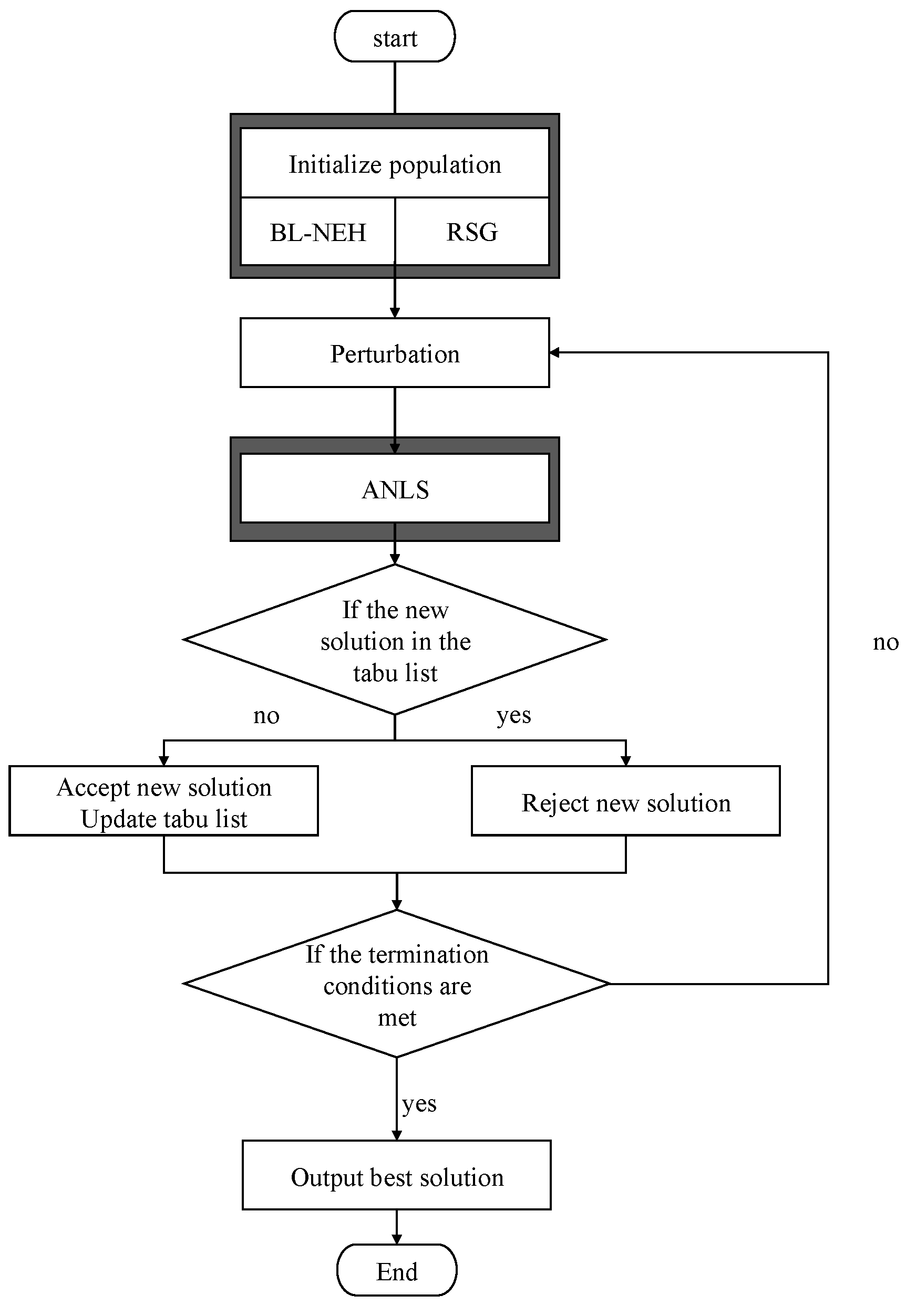
This section introduces the proposed MNATS, with its overall workflow illustrated in Figure 2. MNATS initializes its population using the BL-NEH and Random Solution Generation (RSG) algorithms to ensure high quality and diversity of initial solutions. Under each iteration, the MNATS improves the worst-performing individuals through the ANLS strategy, the ATP strategy use a tabu list to monitor frequently visited solutions, and the perturbation intensity is adjusted accordingly. The final acceptance of new solutions is guided by the simulated annealing criterion. By integrating global exploration and local refinement, MNATS provides an effective solution framework for the DNWFSP.

4.1. Population Initialization

The classic NEH heuristic algorithm [12] has been widely applied to Flow Shop Scheduling Problems, as it can generate high-quality initial solutions. However, when faced with more complex scheduling scenarios, such as the DNWFSP, the NEH algorithm exhibits limitations in balancing job processing times and assessing the global impact of insertion decisions.
To address these limitations, this study proposes an improved NEH algorithm called BL-NEH, which incorporates a job balance factor and a lookahead evaluation mechanism to enhance the overall quality and stability of scheduling solutions, particularly in complex distributed no-wait environments. The BL-NEH algorithm introduces the following two main improvements over the traditional NEH:
(1)
Job Balance Factor:
The balance factor measures the uniformity of a job’s processing times across machines, defined as the ratio of its minimum to maximum processing time. Jobs with highly unbalanced times are more likely to create bottlenecks, since the critical machine dominates completion. By contrast, jobs with higher balance factors are less prone to cause congestion. Prioritizing such jobs helps construct more stable schedules under no-wait constraints, and preliminary tests confirmed that this simple min/max ratio is both effective and computationally inexpensive.
(2)
Lookahead Evaluation:
When constructing the schedule, BL-NEH not only considers the immediate makespan impact of each job insertion but also estimates the influence on subsequent jobs. At each candidate position, it simulates the scheduling of a subset of unscheduled jobs by calculating their average processing times. Half of this minimum average is used as a lower bound for costs. The insertion position with the lowest combined sum of the current makespan and this estimate is selected.
After deriving a globally high-quality job sequence, a greedy allocation strategy is employed to assign jobs to factories. For each job within the sequence, the algorithm assesses all feasible factories and insertion positions, computing the corresponding makespan for every alternative. Subsequently, the job is allocated to the factory–position combination that minimizes the global makespan. This method not only balances the workload across factories but also complies with the no-wait constraints, thus boosting the overall solution quality. The detailed steps of BL-NEH are outlined in Algorithm 1.
Algorithm 1: BL-NEH
Input: J—set of job; P—processing times
Output: X—High-quality initial solution
1: Begin
2:    For each job i in J Do
3:     T i = k = 1 m P i k
4:    Bi = minPik/maxPik
5:    Qi = Ti⋅(1 + Bi)
6:   End For
7:   Sort jobs in descending order of Qi [j1, j2, …, jn]
8:   S = [j1]
9:   For  i = 2 to n  Do
10:    For each possible position pos in S  Do
11:      Insert ji at pos to form S
12:      cost(S′) = Cmax(S′) + lookahead_increment(S′, remaining jobs)
13:    End For
14:    Choose pos* with minimal cost(S′)
15:    Insert ji at pos* in S
16:    End For
17:    X = ∅
18:    For  i = 1 to n  Do
19:    For  j = 1 to f  Do
20:      Evaluate insertion of Si in all positions of factory j
21:    End For
22:    Select factory j* and position pos* with minimal makespan
23:    Insert Si into X at pos* in factory j*
24:   End For
25: End
To ensure population diversity, the RSG is employed during the initialization phase. Specifically, all jobs are randomly permuted first. Subsequently, a greedy allocation strategy is utilized to sequentially assign these jobs to each factory. By repeating this procedure to generate multiple random solutions, the diversity of the initial population is enhanced, thereby providing a broader search space for subsequent evolutionary search. The details are outlined in Algorithm 2.
Algorithm 2: RSG
Input:     n—number of jobs
      f—number of factories
Output:  X—a constructed solution
1: Begin
2:    S = Randomly sort all jobs
3:    Initialize X as empty job sequences for all factories
4:    For  i = 1 to n  Do
5:      For  j = 1 to f  Do
6:       Test inserting job Si at the end of factory j
7:       Compute Cmax (Xj) after insertion
8:      End For
9:       Select factory j* with minimal makespan
10:     Insert job Si at end of j*
11:    End For
12:  End

4.2. ANLS

To further improve solution quality, this paper introduces the ANLS strategy. This strategy employs multiple neighborhood-specific local search algorithms—such as insertion-based, swap-based, and reversal-based search—each optimizing the scheduling sequence from different perspectives. By switching neighborhoods based on the results of different neighborhood searches, ANLS enhances both the depth of local search and the breadth of global exploration.
The ANLS strategy incorporates three primary neighborhood operators. Figure 3 intuitively illustrates following transformation processes corresponding to each operator:
-
Insertion Neighborhood: Remove a job from its current position and insert it into another position within the same factory.
-
Swap Neighborhood: Swap the positions of two distinct jobs within the same factory.
-
Reversion Neighborhood: Reverse the order of a consecutive subsequence of jobs within the same factory.
Figure 3. An example that shows neighborhood operators.
Applsci 15 09840 g003
Different neighborhood structures not only represent different perturbation methods but also correspond to independent local search strategies. To fully exploit the strengths of each neighborhood operator in local optimization, this paper designs local search methods for insertion, swap, and reversion operations. The following sections introduce these three neighborhood-based local search methods in detail.
In the local search of the insertion neighborhood, a Best-Solution-Guided Strategy is designed to use information from high-quality individuals in the current population to guide the local search toward better solutions, thereby accelerating convergence and improving the overall solution quality.
The algorithm is presented in Algorithm 3. First, the solution with the minimum makespan is selected from the current solution set as the reference sequence. Then, insertion operations are sequentially performed on each job in the sequence, and the position with the optimal objective function value is selected from all possible insertion positions. Finally, the updated locally optimal solution is returned.
Algorithm 3: ANLS-Insert Search
Input:    π—current solution set
      X—a newly generated solution to be improved
Output: Xnew—a constructed solution
1: Begin
2:    Xbest = Select solution from π with minimal makespan
3:    Seq = Job sequence of Xbest
4:    For i = 1 to length(Seq) Do
5:      job = Seq [i]
6:      X= Remove job from X
7:      For  pos = 1 to length(Seq) Do
8:        If  posi  then
9:          Insert job at position pos
10:        If Cmax(X′) < Cmax(X) then
11:         Xnew = X
12:        End If
13:        End If
14:      End For
15:    End For
16: End
In this way, the insertion neighborhood operation can not only fully perturb the local structure of the current solution, but it also improves the effectiveness of the search direction under the guidance of the reference solution.
In the multi-neighborhood search framework, the swap neighborhood is a commonly used local search operation [36]. Its basic idea is to swap the positions of any two jobs within the same factory to generate a new scheduling solution. The swap neighborhood can rearrange the job sequence in a small range to escape from the current local optimal solution. Details are shown in Algorithm 4.
Algorithm 4: ANLS—Swap Search
Input:    π—current solution set
            X—a newly generated solution to be improved
Output:  Xnew—a constructed solution
1: Begin
2:    Xnew = X
3:    For each factory F in X Do
4:     Seq = Job sequence of  F
5:     For i = 1 to length(Seq) − 1 Do
6:       For  j = i + 1 to length(Seq) Do
7:           Seq′ = Swap Seq [i] and Seq [j]
8:           X′ = X with Seq′ for factory F
9:           If Cmax(X’) < Cmax (Xnew) then
10:           Xnew = X
11:         End If
12:       End For
13:     End For
14:   End For
15: End
Reverse neighborhood is a local search operator with strong structural perturbation capability [37]. Its basic idea is as follows: within the same factory, select any sub-interval [i, j] (i < j) from the job sequence and reverse the job order within this interval to form a new scheduling solution. Compared with simple swap or insertion, this operation enables a larger range of sequence reconstruction, helping escape local optimal traps and expanding the solution space. Details are shown in Algorithm 5.
Algorithm 5: ANLS—Reverse Search
Input:    π—current solution set
            X—a newly generated solution to be improved
Output:  Xnew—a constructed solution
1: Begin
2:    Xnew = X
3:    For each factory F in X Do
4:     Seq = Job sequence of  F
5:     For  i = 1 to length(Seq) − 1 Do
6:         For  j = i + 1 to length(Seq) Do
7:         Seq′ = Seq
8:      Reverse Seq′ [i..j] // reverse the subsequence between positions i and j
9:         X′ = X with Seq′ for factory F
10:       If  Cmax(X′) < Cmax (Xnew) then
11:         Xnew = X
12:       End If
13:      End For
14:     End For
15:    End For
16: End
Through systematic enumeration and evaluation of all possible reverse operations, the ANLS-Reverse Search can significantly expand the search scope while maintaining structural rationality, serving as an important means to improve search depth.
In summary, the proposed ANLS strategy integrates three representative neighborhood structures, which are insertion, swap, and reversion. The insertion neighborhood is further enhanced by an elite-guided strategy, while the swap and reversion neighborhoods focus on broader structural perturbations and are retained as non-guided strategies to preserve search diversity. By combining these heterogeneous operators with adaptive switching, ANLS can effectively balance local intensification and global diversity. Among them, insertion serves as the primary search operator, while swap and reversion act as auxiliary operators that are activated when insertion becomes trapped in local optima; after improvement is obtained, the search returns to insertion. The complete procedure of ANLS is presented in Algorithm 6.
Algorithm 6: ANLS
Input:    π—current solution set
            X—a newly generated solution to be improved
Output: Xnew—a constructed solution
1: Begin
2:    Xnew = X
3:    Ntypes = {Insert, Swap, Reverse}
4:    k = 1
5:    While  k ≤ length(Ntypes) Do
6:       N = Ntypes [k]
7:       Xtemp = Apply neighborhood search N to Xnew
8:       If Xtemp not in tabu list T and Cmax (Xtemp) < Cmax (Xnew) then
9:         Xnew = Xtemp
10:        Update Tabu List T with Xtemp
11:         k = 1     // reset to Insert next round
12:        Break
13:      Else
14:         k = k + 1    // try next operator
15:     End If
16:    End While
17: End

4.3. ATP

To prevent the algorithm from being trapped in local optima and to enhance its global exploration capability, this paper proposes the ATP. The detailed procedure is summarized in Algorithm 7. In each iteration, ATP randomly selects a solution from the current population as the perturbation target. It identifies the key factory (the factory with the longest current makespan), exchanges a random number of jobs from this factory with those from another randomly selected factory, and generates a structurally perturbed solution. This process is repeated several times, and the solution with the smallest makespan is retained for subsequent neighborhood search.
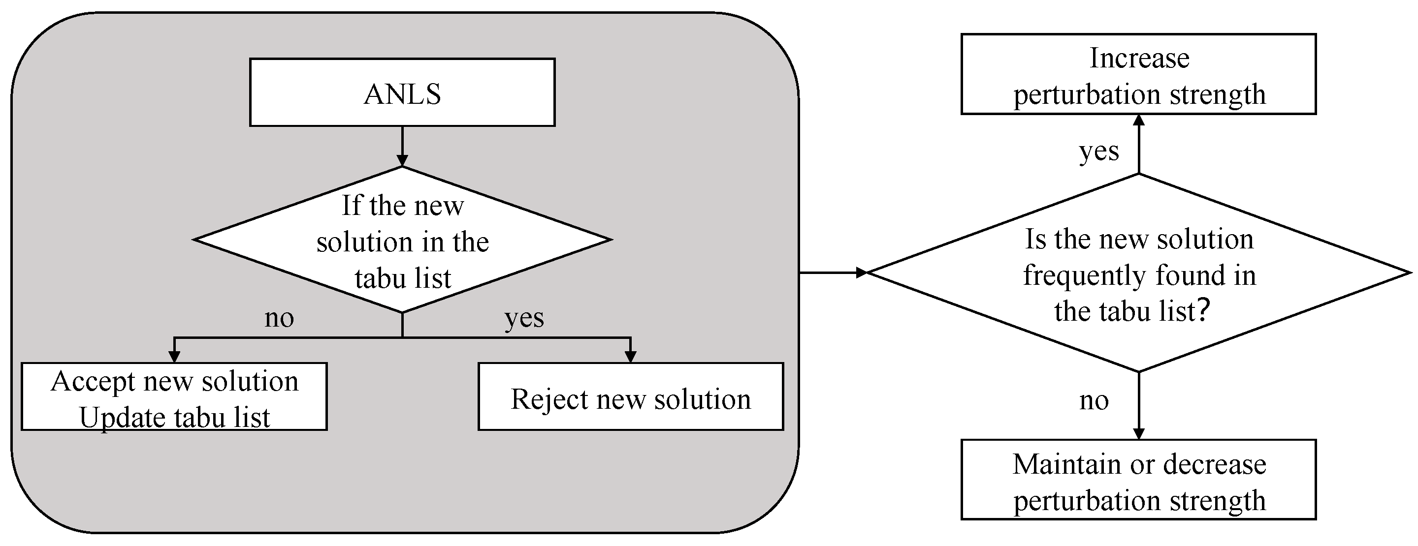
To avoid redundant or ineffective perturbations, a hash-based tabu list is introduced to track recently visited solutions. Each solution is hashed for fast lookup and stored in a fixed-length tabu list. If a newly generated solution is frequently found in the tabu list, then the ATP will adaptively intensify the perturbation to explore more diverse solution regions. Conversely, if few tabu hits occur, then the perturbation intensity is reduced to save computational cost. The adaptation is controlled by the parameter r ∈ (0, 1], where r simultaneously determines the number of perturbation attempts and the maximum swap size in ATP. After each iteration, r is updated based on the tabu hit rate as follows:
r min ( 1 , r ( 1 + γ ) ) , if   hit   rate h h i g h max ( r m i n , r ( 1 γ ) ) , if   hit   rate h l o w
where hlow and hhigh are predefined thresholds, γ is the adjustment factor, and r is clipped within [rmin, 1].
Algorithm 7: ATP
Input:  π—current solution set
    X—a newly generated solution to be improved
    T—tabu list
    r—perturbation intensity
    κ—max swap size
    l—max perturbation size
Output: Xnew—a constructed solution
1: Begin
2:    Xnew = X
3:    Identify the key factory F*
4:    C = ∅; skipped = 0; i = 1
5:    While  ir × l  Do
6:      Randomly select k ∈ {1, …, κ × r}
7:      Randomly pick k jobs from F* and k jobs from another factory F
8:      Xtemp = Exchange these jobs between F* and F
9:      If hash(Xtemp) ∈ T  then
10:        skipped = skipped + 1; i = i + 1; Continue
11:       End If
12:       Evaluate Cmax(Xtemp)
13:       C = C ∪ {Xtemp}
14:       i = i + 1
15:     End While
16:     Xnew = getmin Cmax(C)
17:     hit_rate = skipped/r × l
18:     intensity adaptation (hit_rate)
19:     Update T with Xnew
20:     Return Xnew
21: End
This is also illustrated in Figure 4. Regarding tabu list feedback from ANLS, the tabu list is not only employed in ANLS to avoid revisiting previously explored solutions, but it also provides feedback to ATP. By adaptively adjusting the perturbation strength based on historical feedback, ATP enhances the algorithm’s ability to escape local optima while preserving diversity and promoting robust global search.

4.4. Acceptance Criterion

To enhance the algorithm’s ability to escape local optima, a simulated annealing (SA) acceptance criterion is incorporated into the insertion neighborhood search. Specifically, new solutions that improve the objective function are always accepted, while worse solutions are accepted with a probability determined by the SA criterion. This probability decreases as the search progresses, balancing exploration and exploitation. The acceptance probability is calculated as follows:
P = 1 , Δ < 0 e x p ( Δ T ) , Δ 0
where Δ is the difference in objective value between the new and current solutions, and T is the temperature parameter.
This mechanism helps the algorithm avoid premature convergence and improves overall performance.

4.5. Computational Complexity

Evaluating a distributed no-wait schedule requires O(mn) time, since each of the n jobs is processed sequentially on m machines. For the BL-NEH initializer, job statistics and sorting take O(nm+nlogn), while sequence construction and factory assignment can be performed in O(mn2) using incremental evaluation. In the ANLS phase, insertion and swap neighborhoods examine O(n2) moves per factory, leading to O(mn2) overall, whereas full reversal yields a pessimistic bound of O(mn3). The ATP perturbation generates r × l candidates per call, with each evaluated in O(mn), resulting in O(rlmn). Consequently, initializing P solutions costs O(Pmn2), and each iteration that improves c individuals requires O(c(mn2+rlmn)). The total time complexity is therefore shown as follows:
O ( m n 2 ( P + T c ) + T c r l m n )
This is typically dominated by the O(mn2(P+Tc)) term. In practice, only the affected factory must be recomputed after a move(O(mn)); thus, the average computational burden is significantly lower than the theoretical worst-case bound. Therefore, the MNATS exhibits high scalability.

5. Experiments

In this section, to verify the effectiveness and superiority of the proposed MNATS in solving the DNWFSP, a series of experiments are conducted. This section presents the experimental setup, evaluation metrics, ablation studies, parameter analysis, and comparative analyses of algorithm performance.

5.1. Experimental Setup

This experiment was implemented on a Windows 11 system with an Intel Ultra 9 185H 2.50 GHz processor and 32 GB RAM, and the algorithms were coded in C++. To ensure the fairness and reproducibility of experimental results, all algorithms were independently run five times under the same operating environment and constraints, with the average and optimal values recorded for analysis.
The experiments are based on the Taillard benchmark instances [38], which are among the most widely used testbeds for flow shop and distributed scheduling research. Introduced in 1993, these instances were specifically designed to mimic realistic industrial scheduling environments while providing a standardized and reproducible platform for algorithm comparison. Due to their diversity in terms of jobs, machines, and factories, Taillard instances have become the de facto standard in the literature for over two decades, allowing fair comparisons across a wide range of heuristic and metaheuristic approaches. Specifically, the number of jobs is set as n = {20, 50, 100, 200, 500}, the number of factories as f = {2, 3, 4, 5, 6}, and the number of processes as m = {5, 10, 20}. These settings are designed to investigate the stability and scalability of the algorithms. No modifications were made to these instances, thereby ensuring direct comparability and reproducibility with previous studies.
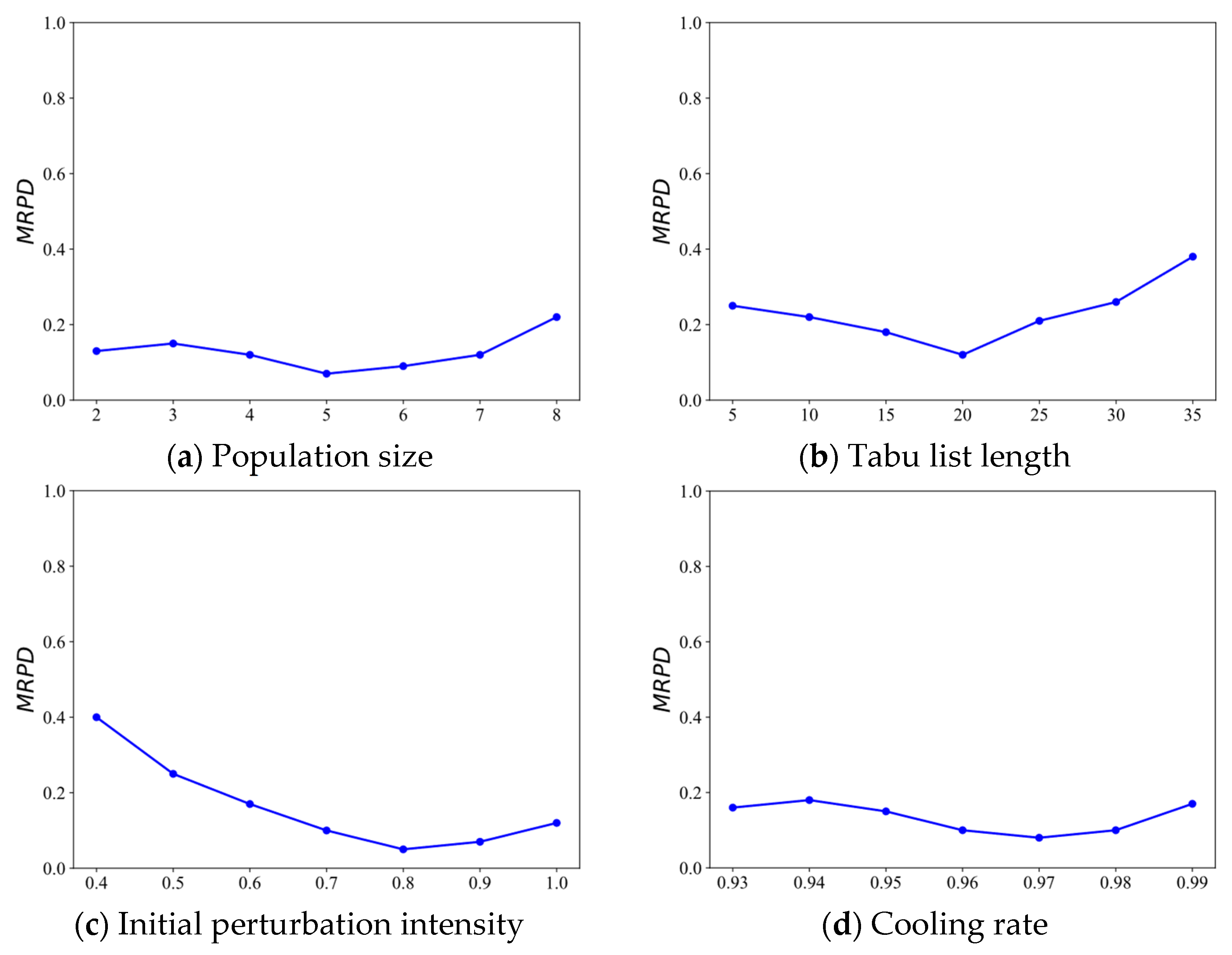
Some of the key parameters of MNATS were selected with reference to previous studies [39], while others were determined through preliminary trials. The parameters are summarized in Table 2. The population size was set to 5 to balance diversity with computational cost. The tabu list length was fixed at 20, following common practice in tabu search to avoid cycling without incurring high memory cost. The initial perturbation intensity was set to 0.8, since lower values reduced diversification while higher values caused instability in pilot experiments. The cooling rate of 0.97, widely used in metaheuristics, was chosen to provide a smooth trade-off between exploration and exploitation. The sensitivity of these key parameters is further analyzed in Section 5.6.

5.2. Experimental Evaluation Metrics

To fairly compare the scheduling performance of different algorithms across various instances, this paper adopts the Relative Percentage Deviation (RPD) as the primary evaluation metric, which is defined as follows:
RPD = C max C b e s t C b e s t × 100 %
where Cmax is the makespan obtained by the algorithm for a problem instance, and Cbest is the minimum makespan achieved by all algorithms for that instance.
Obviously, a smaller RPD value indicates that the algorithm is closer to optimal performance. For multiple instances, the mean RPD can be used to compare the overall performance of algorithms.

5.3. Comparative Experiment

To evaluate the performance of the proposed MNATS algorithm, we compare it with both classical and state-of-the-art algorithms, including the Iterated Greedy algorithm (IG) [40]; the discrete Artificial Bee Colony algorithm (ABC) [33]; and the Population-based Iterated Greedy Algorithm (PBIGA) [41].
As shown in Table 3, MNATS demonstrates significantly superior performance as the number of iterations increases, with its advantage becoming more pronounced under higher iteration thresholds. Although MNATS generally outperforms all baseline algorithms, we observed a few exceptions in the short-run setting of 100 iterations with f = 4 and f = 6, where PBIGA achieved slightly better average RPD values. This can be explained by the strong intensification ability of PBIGA, which enables it to exploit good solutions rapidly under very limited iteration budgets. In contrast, MNATS is designed with adaptive perturbation and multi-neighborhood mechanisms that require more iterations to take full effect. As the number of iterations increases, MNATS consistently surpasses PBIGA, demonstrating its superior robustness and long-term performance.
When the iteration count reaches 200 or more, MNATS consistently outperforms the other three algorithms across all test instances. Its RPD values remain the lowest throughout, and under 300 iterations, most results are close to zero. Importantly, the reported standard deviations indicate that MNATS not only achieves lower average RPD values but also maintains smaller variability across independent runs. This highlights that MNATS is more robust and stable than the baselines, confirming that the collaborative multi-neighborhood design and adaptive strategies effectively enhance global solution quality and convergence accuracy.
To further validate the statistical significance of the observed improvements, the Wilcoxon signed-rank test was performed between MNATS and each baseline algorithm across all benchmark instances. The results are summarized in Table 4. As shown, MNATS consistently achieves significantly better performance than IG, ABC, and PBIGA, all with corresponding p-values below 0.01. These results confirm that the superiority of MNATS is not due to random variation but is statistically significant at the 1% level, meaning that the performances of the compared algorithms have significant differences.
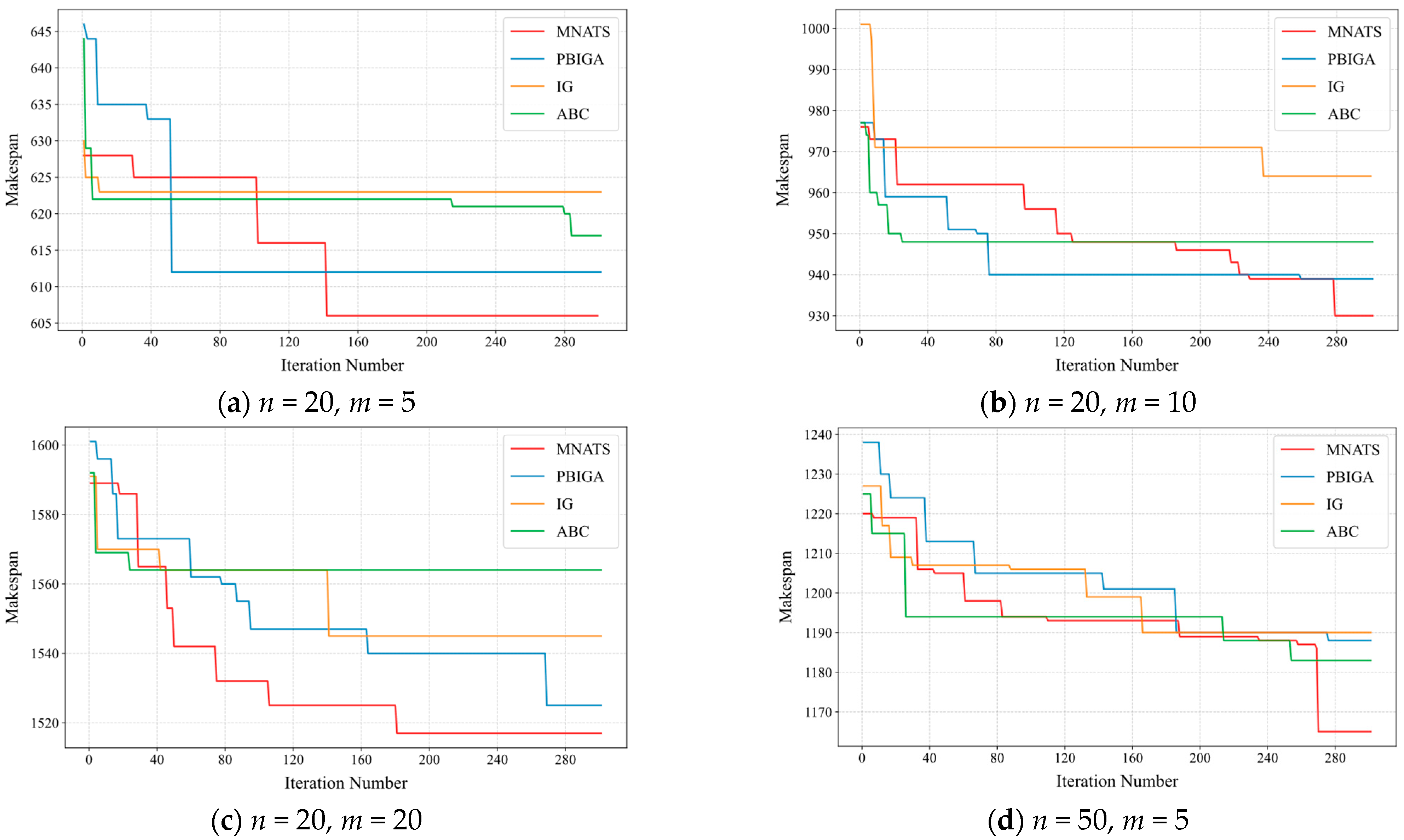
To further evaluate the convergence behavior of the proposed MNATS algorithm, convergence curves of MNATS and the other three comparative algorithms were plotted for datasets of different sizes. In each experiment, the makespan value found by each algorithm was recorded at each iteration, and the results are shown in Figure 5.
The figures depict the convergence curves of these algorithms across test scenarios of different scales. It can be observed that MNATS demonstrates significant competitiveness among the compared algorithms; it achieves optimal solutions in all test cases and converges to high-quality solutions within a reasonable number of iterations. In most cases, both the convergence speed and final results of IG and ABC are inferior to those of MNATS. As the problem scale increases, MNATS’ advantage becomes increasingly prominent. In summary, the proposed MNATS is effective and efficient for solving the DNWFSP.

5.4. Runtime Analysis

To visually demonstrate the differences in operational efficiency between MNATS and comparative algorithms, this paper normalizes the average running time of MNATS to 1 and calculates the relative running time ratios of the remaining algorithms under the same number of iterations.
As shown in Table 5, IG and ABC are generally 20–30% faster than MNATS but suffer from lower accuracy and a higher risk of premature convergence, while PBIGA requires about 130% of the runtime of MNATS without achieving comparable solution quality. Although MNATS takes slightly longer than IG and ABC, it offers a much better balance of accuracy, stability, and adaptability to complex environments, reflecting stronger comprehensive performance.
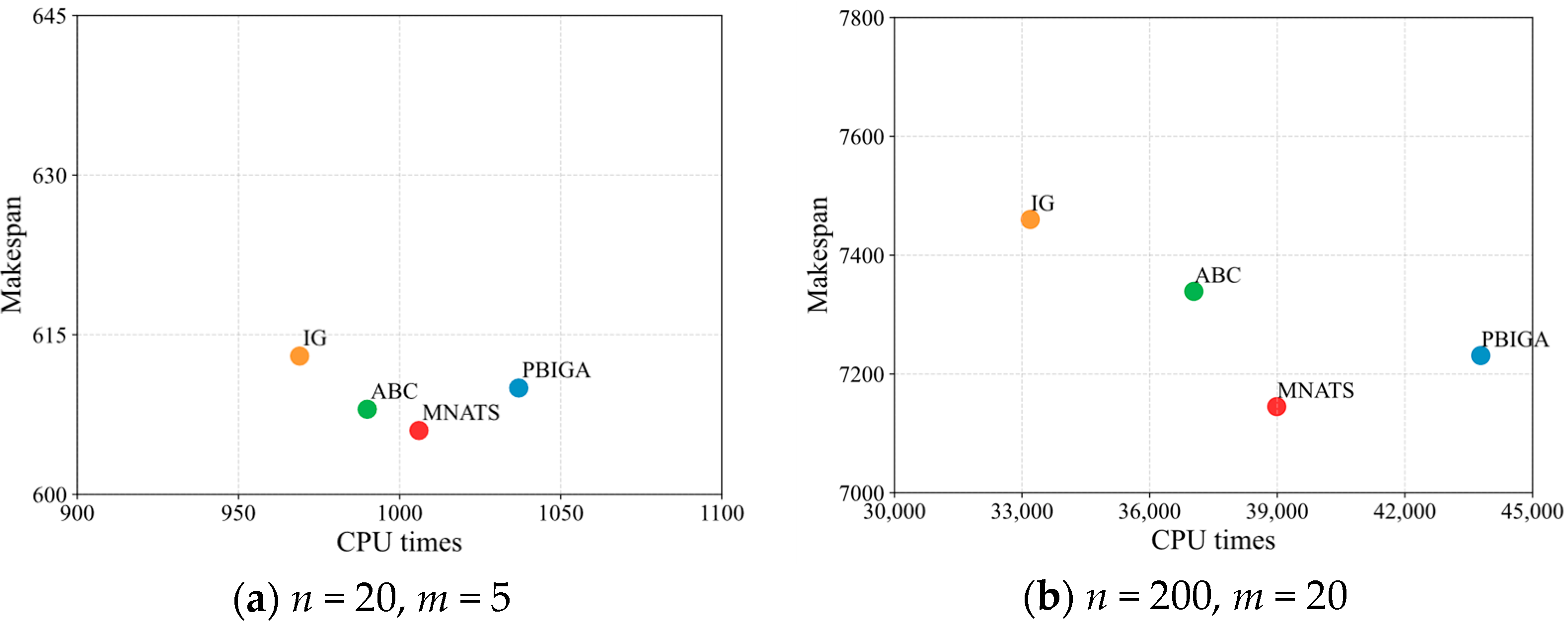
In addition, we further provide absolute runtime comparisons on Taillard instances with three factories. Figure 6 shows the results for a small-scale instance and a large-scale instance. It can be observed that MNATS achieves lower makespans than the baselines while maintaining competitive runtime efficiency in both cases. These findings confirm that the superior solution quality of MNATS is not obtained at the expense of prohibitive computational cost.

5.5. Ablation Experiments

To deeply analyze the role of each module in MNATS, the following three variants are designed for ablation tests:
  • MNATS w/o BL-NEH: Removes the BL-NEH module and uses traditional NEH initialization.
  • MNATS ANLS-Insert/ANLS-Swap/ANLS-Reverse: Retains only one neighborhood operator in ANLS to evaluate the contribution of each neighborhood separately.
  • MNATS w/o ATP: Removes the tabu list and uses a fixed perturbation strength.
As shown in Table 6, all three modules make significant contributions to the performance of MNATS. For instance, in the case of f = 5, the complete MNATS achieves an RPD of 0.23. When the BL-NEH module is removed, the RPD increases to 0.38; in the single-neighborhood variants, insert performs best, while swap and reverse are much worse. This confirms that the insert operator contributes the majority of local improvements, while swap and reverse mainly play auxiliary roles in diversifying the search and helping MNATS escape local optima. Similarly, removing the ATP also leads to a noticeable increase in RPD to 0.64.
These results demonstrate that BL-NEH, ANLS, and ATP work together to improve solution quality and maintain search diversity. Insert is the main contributor to local intensification, while swap and reverse serve as auxiliary operators when insert stagnates, confirming the necessity of combining them under the adaptive framework.

5.6. Sensitivity Analysis of Key Parameters

To elucidate how key parameters influence the performance of the MNATS algorithm, we conducted a sensitivity analysis on the four main parameters listed in Table 2. Each parameter was varied independently over a discrete grid while fixing the others at their default values. For each setting, we ran five independent trials and reported the MRPD. Figure 7 illustrates the impact of these parameters.
As shown in Figure 7a, population sizes of 4–5 yield the lowest MRPD, with the optimum at 5. Too small a population leads to insufficient diversity and unstable results, while an excessively large size increases computational overhead and reduces efficiency. In Figure 7b, a tabu list length of 20 achieves the best performance; a short tabu list fails to prevent cycling, whereas an overly long list restricts revisitation flexibility. The performance remains stable in the range of 15–25. Figure 7c indicates that an initial perturbation intensity of 0.8 provides the most effective balance between structural disruption and guided search. Figure 7d shows that a cooling rate between 0.96 and 0.97 achieves the best performance, as it improves the global search ability of the acceptance criterion.
In summary, MNATS achieves its best performance when the population size is set to 5, the tabu list length is set to 20, the initial perturbation intensity is set to 0.8, and the cooling rate is set to 0.97. Moreover, the results remain stable within small neighborhoods of these settings, confirming that MNATS is robust to moderate parameter changes and that the chosen defaults lie in a near-optimal region.

6. Conclusions

This paper addresses the DNWFSP and proposes the MNATS algorithm. By combining a job balance factor with lookahead evaluation, MNATS generates high-quality initial solutions, while the Adaptive Neighborhood Local Search and Adaptive Tabu-Guided Perturbation modules jointly enhance intensification and diversification. Experimental results on Taillard benchmark instances indicate that MNATS achieves better overall performance than representative baselines such as IG, ABC, and PBIGA, with statistically significant improvements in both solution accuracy and stability. Moreover, the scalability of MNATS is validated on large-scale instances, highlighting its potential applicability to complex distributed scheduling environments.
In addition to these advantages, MNATS also has certain limitations. It requires a relatively large number of iterations to fully exploit its adaptive mechanisms, which may increase computational cost in time-constrained applications. Its performance is influenced by parameters such as tabu tenure, perturbation intensity, and the balance factor, which—although shown to be robust—still require careful tuning. Moreover, the current evaluation is limited to Taillard benchmark instances; real industrial data and additional practical factors such as transportation times, resource balancing, and energy consumption remain to be addressed.
In future research, our work will continue to build upon MNATS as a foundation, and we will address the limitations (e.g., ignoring transport time, load balancing) as a critical step toward tackling more practical and challenging scenarios. First, greater attention will be devoted to validating its performance on real-world industrial data and extending the evaluation beyond benchmark instances. Another important direction is the incorporation of multi-objective criteria, particularly energy efficiency and sustainability, which have become central in modern manufacturing systems. At the methodological level, learning-based approaches are emerging as a powerful complement to traditional metaheuristics. On the one hand, reinforcement learning has been integrated with evolutionary and swarm-based strategies to improve convergence and address multi-objective goals such as makespan and energy efficiency [42,43]. On the other hand, deep reinforcement learning frameworks, often combined with graph neural networks, have demonstrated strong adaptability in distributed environments and have shown promise in handling dynamic and uncertain scheduling scenarios [44]. By incorporating these advances, our subsequent research will focus on developing sustainable, adaptive, and resilient distributed scheduling systems.

Author Contributions

Z.Z.: Writing—original draft preparation, methodology; W.Z.: Investigation, formal analysis, resources; H.Z.: Writing—review and editing, supervision; X.B.: Con-ceptualization, supervision. All authors have read and agreed to the published version of the manuscript.

Funding

This work was supported in part by the National Key Research and Development Program (2023YFB3307400).

Institutional Review Board Statement

Not applicable.

Informed Consent Statement

Not applicable.

Data Availability Statement

The code used in this study and datasets are available from the corresponding author upon reasonable request.

Conflicts of Interest

The authors declare no conflicts of interest.

References

  1. Lin, S.W.; Ying, K.C. Minimizing makespan for solving the distributed no-wait flowshop scheduling problem. Comput. Ind. Eng. 2016, 99, 202–209. [Google Scholar] [CrossRef]
  2. Aldowaisan, T.; Allahverdi, A. Minimizing total tardiness in no-wait flowshops. Found. Comput. Decis. Sci. 2012, 37, 149–162. [Google Scholar] [CrossRef]
  3. Rajendran, C. A no-wait flowshop scheduling heuristic to minimize makespan. J. Oper. Res. Soc. 1994, 45, 472–478. [Google Scholar] [CrossRef]
  4. Hall, N.G.; Sriskandarajah, C. A survey of machine scheduling problems with blocking and no-wait in process. Oper. Res. 1996, 44, 510–525. [Google Scholar] [CrossRef]
  5. Garey, M.R.; Johnson, D.S.; Sethi, R. The complexity of flowshop and jobshop scheduling. Math. Oper. Res. 1976, 1, 117–129. [Google Scholar] [CrossRef]
  6. Wang, B.; Han, K.; Spoerre, J.; Zhang, C. Integrated product, process and enterprise design: Why, what and how? In Integrated Product, Process and Enterprise Design; Springer: Boston, MA, USA, 1997; pp. 1–20. [Google Scholar]
  7. Kahn, K.B. The PDMA Handbook of New Product Development; Wiley: Hoboken, NJ, USA, 2013. [Google Scholar]
  8. Tseng, L.Y.; Lin, Y.T. A hybrid genetic algorithm for no-wait flowshop scheduling problem. Int. J. Prod. Econ. 2010, 128, 144–152. [Google Scholar] [CrossRef]
  9. Zhang, W.; Geng, H.; Li, C.; Gen, M.; Zhang, G.; Deng, M. Q-learning-based multi-objective particle swarm optimization with local search within factories for energy-efficient distributed flow-shop scheduling problem. J. Intell. Manuf. 2023, 36, 185–208. [Google Scholar] [CrossRef]
  10. Komaki, M.; Malakooti, B. General variable neighborhood search algorithm to minimize makespan of the distributed no-wait flow shop scheduling problem. Prod. Eng. 2017, 11, 315–329. [Google Scholar] [CrossRef]
  11. Allali, K.; Aqil, S.; Belabid, J. Distributed no-wait flow shop problem with sequence dependent setup time: Optimization of makespan and maximum tardiness. Simul. Model. Pr. Theory 2022, 116, 102455. [Google Scholar] [CrossRef]
  12. Nawaz, M.; Enscore, E.E., Jr.; Ham, I. A heuristic algorithm for the m-machine, n-job flow-shop sequencing problem. Omega 1983, 11, 91–95. [Google Scholar] [CrossRef]
  13. Zeng, Q.-Q.; Li, J.-Q.; Li, R.-H.; Huang, T.-H.; Han, Y.-Y.; Sang, H.-Y. Improved NSGA-II for energy-efficient distributed no-wait flow-shop with sequence-dependent setup time. Complex Intell. Syst. 2022, 9, 825–849. [Google Scholar] [CrossRef]
  14. Aggoune, R. Minimizing the makespan for the flow shop scheduling problem with availability constraints. Eur. J. Oper. Res. 2004, 153, 534–543. [Google Scholar] [CrossRef]
  15. Koulamas, C.; Kyparisis, G.J. Two-stage no-wait proportionate flow shop scheduling with minimal service time variation and optional job rejection. Eur. J. Oper. Res. 2022, 305, 608–616. [Google Scholar] [CrossRef]
  16. Utama, D.M.; Umamy, S.Z.; Al-Imron, C.N. No-wait flow shop scheduling problem: A systematic literature review and bibli-ometric analysis. RAIRO-Oper. Res. 2024, 58, 1281–1313. [Google Scholar] [CrossRef]
  17. Wang, S.-Y.; Wang, L.; Liu, M.; Xu, Y. An effective estimation of distribution algorithm for solving the distributed permutation flow-shop scheduling problem. Int. J. Prod. Econ. 2013, 145, 387–396. [Google Scholar] [CrossRef]
  18. Becker, T.; Neufeld, J.; Buscher, U. The distributed flow shop scheduling problem with inter-factory transportation. Eur. J. Oper. Res. 2024, 322, 39–55. [Google Scholar] [CrossRef]
  19. Miyata, H.H.; Nagano, M.S. An iterated greedy algorithm for distributed blocking flow shop with setup times and maintenance operations to minimize makespan. Comput. Ind. Eng. 2022, 171, 108366. [Google Scholar] [CrossRef]
  20. Avci, M.; Avci, M.G.; Hamzadayı, A. A branch-and-cut approach for the distributed no-wait flowshop scheduling problem. Comput. Oper. Res. 2022, 148, 106009. [Google Scholar] [CrossRef]
  21. Bäck, T.; Schwefel, H.-P. An Overview of Evolutionary Algorithms for Parameter Optimization. Evol. Comput. 1993, 1, 1–23. [Google Scholar] [CrossRef]
  22. Hussain, K.; Salleh, M.N.M.; Cheng, S.; Shi, Y. Metaheuristic research: A comprehensive survey. Artif. Intell. Rev. 2018, 52, 2191–2233. [Google Scholar] [CrossRef]
  23. Ruiz, R.; Maroto, C.; Alcaraz, J. Two new robust genetic algorithms for the flowshop scheduling problem. Omega 2006, 34, 461–476. [Google Scholar] [CrossRef]
  24. Engelbrecht, A.P.; Grobler, J.; Langeveld, J. Set based particle swarm optimization for the feature selection problem. Eng. Appl. Artif. Intell. 2019, 85, 324–336. [Google Scholar] [CrossRef]
  25. Chen, R.M.; Lo, S.T.; Wu, C.L.; Lin, T.H. An effective ant colony optimization-based algorithm for flow shop scheduling. In Proceedings of the 2008 IEEE Conference on Soft Computing in Industrial Applications, Muroran, Japan, 25–27 June 2008; IEEE: Piscataway, NJ, USA; pp. 101–106. [Google Scholar]
  26. Zhang, W.; Wang, Y.; Yang, Y.; Gen, M. Hybrid multiobjective evolutionary algorithm based on differential evolution for flow shop scheduling problems. Comput. Ind. Eng. 2019, 130, 661–670. [Google Scholar] [CrossRef]
  27. Engin, O.; Güçlü, A. A new hybrid ant colony optimization algorithm for solving the no-wait flow shop scheduling prob-lems. Appl. Soft Comput. 2018, 72, 166–176. [Google Scholar] [CrossRef]
  28. Nejjarou, O.; Aqil, S.; Lahby, M. Hybrid meta-heuristic solving no-wait flow shop scheduling minimizing maximum tardiness. Evol. Intell. 2024, 17, 3935–3959. [Google Scholar] [CrossRef]
  29. Han, X.; Han, Y.; Chen, Q.; Li, J.; Sang, H.; Liu, Y.; Pan, Q.; Nojima, Y. Distributed flow shop scheduling with sequence-dependent setup times using an improved iterated greedy algorithm. Complex Syst. Model. Simul. 2021, 1, 198–217. [Google Scholar] [CrossRef]
  30. Lu, C.; Huang, Y.; Meng, L.; Gao, L.; Zhang, B.; Zhou, J. A Pareto-based collaborative multi-objective optimization algorithm for energy-efficient scheduling of distributed permutation flow-shop with limited buffers. Robot. Comput. Manuf. 2022, 74, 102277. [Google Scholar] [CrossRef]
  31. Khurshid, B.; Maqsood, S.; Khurshid, Y.; Naeem, K.; Khalid, Q.S. A hybridization of evolution strategies with iterated greedy algorithm for no-wait flow shop scheduling problems. Sci. Rep. 2024, 14, 1–22. [Google Scholar] [CrossRef] [PubMed]
  32. Pan, Y.; Gao, K.; Li, Z.; Wu, N. A novel evolutionary algorithm for scheduling distributed no-wait flow shop problems. IEEE Trans. Syst. Man, Cybern. Syst. 2024, 54, 3694–3704. [Google Scholar] [CrossRef]
  33. Li, H.; Li, X.; Gao, L. A discrete artificial bee colony algorithm for the distributed heterogeneous no-wait flowshop scheduling problem. Appl. Soft Comput. 2021, 100, 106946. [Google Scholar] [CrossRef]
  34. Zhu, N.; Zhao, F.; Yu, Y.; Wang, L. A cooperative learning-aware dynamic hierarchical hyper-heuristic for distributed heterogeneous mixed no-wait flow-shop scheduling. Swarm Evol. Comput. 2024, 90, 101668. [Google Scholar] [CrossRef]
  35. Zhang, X.-J.; Li, J.-Q.; Liu, X.-F.; Tian, J.; Duan, P.-Y.; Tan, Y.-Y. A hybrid whale optimization algorithm for distributed no-wait flow-shop scheduling problem with batch delivery. J. Intell. Fuzzy Syst. 2024, Preprint, 1–14. [Google Scholar] [CrossRef]
  36. An, Y.; Chen, X.; Gao, K.; Li, Y.; Zhang, L. Multiobjective flexible job-shop rescheduling with new job insertion and machine preventive maintenance. IEEE Trans. Cybern. 2022, 53, 3101–3113. [Google Scholar] [CrossRef]
  37. Li, J.-Q.; Pan, Q.-K.; Wang, F.-T. A hybrid variable neighborhood search for solving the hybrid flow shop scheduling problem. Appl. Soft Comput. 2014, 24, 63–77. [Google Scholar] [CrossRef]
  38. Taillard, E. Benchmarks for basic scheduling problems. Eur. J. Oper. Res. 1993, 64, 278–285. [Google Scholar] [CrossRef]
  39. Avci, M. An effective iterated local search algorithm for the distributed no-wait flowshop scheduling problem. Eng. Appl. Artif. Intell. 2023, 120, 105921. [Google Scholar] [CrossRef]
  40. Shao, W.; Pi, D.; Shao, Z. Optimization of makespan for the distributed no-wait flow shop scheduling problem with iterated greedy algorithms. Knowl.-Based Syst. 2017, 137, 163–181. [Google Scholar] [CrossRef]
  41. Zhao, F.; Xu, Z.; Wang, Q. A population-based iterated greedy algorithm for distributed no-wait flow-shop scheduling problem. In Proceedings of the 2023 26th International Conference on Computer Supported Cooperative Work in Design (CSCWD), Rio de Janeiro, Brazil, 24–26 May 2023; pp. 715–720. [Google Scholar]
  42. Zhao, F.; Yin, F.; Wang, L.; Yu, Y. A co-evolution algorithm with dueling reinforcement learning mechanism for the energy-aware distributed heterogeneous flexible flow-shop scheduling problem. IEEE Trans. Syst. Man, Cybern. Syst. 2024, 55, 1794–1809. [Google Scholar] [CrossRef]
  43. Huang, J.-P.; Gao, L.; Li, X.-Y. An end-to-end deep reinforcement learning method based on graph neural network for distributed job-shop scheduling problem. Expert Syst. Appl. 2023, 238, 121756. [Google Scholar] [CrossRef]
  44. Wu, X.; Yan, X.; Guan, D.; Wei, M. A deep reinforcement learning model for dynamic job-shop scheduling problem with uncertain processing time. Eng. Appl. Artif. Intell. 2024, 131, 107790. [Google Scholar] [CrossRef]
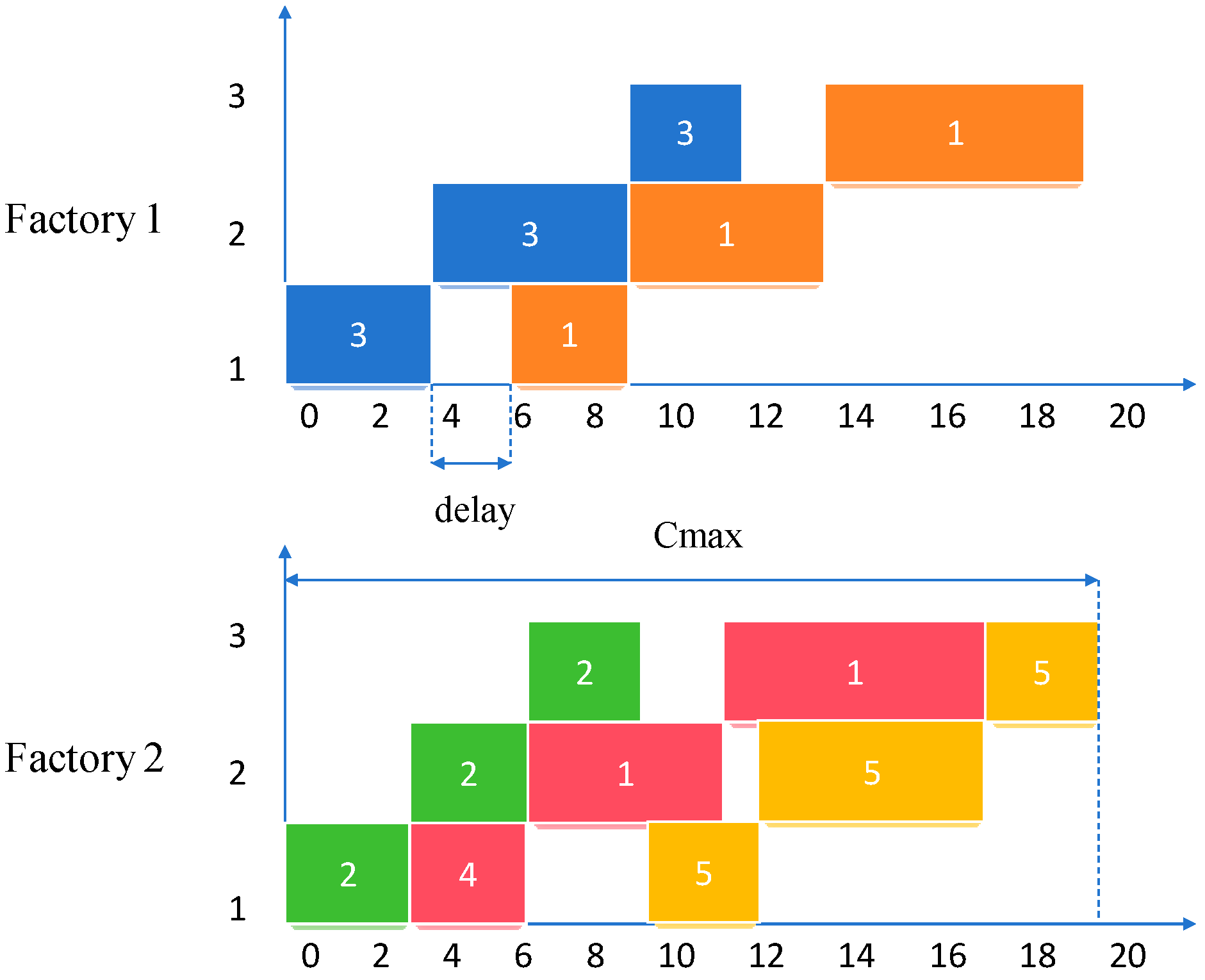
Figure 1. Example Gantt chart of the DNWFSP illustrating the no-wait constraint. Jobs are scheduled across two factories, with each rectangle representing an operation. The horizontal axis denotes processing time; the vertical axis denotes machines.
Applsci 15 09840 g001
Figure 2. The overall framework of MNATS.
Applsci 15 09840 g002
Figure 4. Tabu list feedback from ANLS.
Applsci 15 09840 g004
Figure 5. Convergence curves of MNATS and the baseline algorithms on Taillard benchmark instances with three factories. Lower makespan values indicate better performance.
Applsci 15 09840 g005
Figure 6. Comparison of runtime and makespan for MNATS and the baseline algorithms on Taillard benchmark instances with three factories.
Applsci 15 09840 g006
Figure 7. Sensitivity analysis of key parameters in MNATS.
Applsci 15 09840 g007
Table 1. Symbols of the DNWFSP.
SymbolsDescription
Parameters and Sets
πSolution
iIndex for jobs, where i = 1 , 2 , , n
jIndex for factories, where j = 1 , 2 , , f
kIndex for machines, where k = 1 , 2 , , m
J = {J1, J2, …, Jn}Set of jobs, containing n jobs
F = {F1, F2, …, Ff}Set of factories, with a total of f factories
M = {M1, M2, …, Mm}Set of machines in each factory, with m processing stages
Pi,kProcessing time of job Ji on machines k
πijThe i-th job in the processing sequence of factory Fj
CmaxMaximum completion time among all jobs in all factories
d π i 1 , j , π i , j The delay between the start time of job πi−1 ,j and job πij on the first machine
xi,jBinary variable: xi,j = 1 if job Ji is assigned to factory Fj;
otherwise xi,j = 0
Table 2. Parameter configuration in the experiment.
Parameter Setting
Population size 5
Tabu list length 20
Initial perturbation intensity0.8
Cooling rate0.97
Table 3. The RPD of MNATS and three comparative algorithms. Lower RPD values indicate better performance, and the best results in each row are highlighted in bold.
Iteration TimesfIGABCPBIGAMNATS
10024.23 ± 0.283.81 ± 0.251.54 ± 0.141.67 ± 0.12
34.15 ± 0.273.52 ± 0.222.28 ± 0.191.58 ± 0.11
44.02 ± 0.303.33 ± 0.231.91 ± 0.161.95 ± 0.14
53.88 ± 0.263.15 ± 0.202.55 ± 0.212.31 ± 0.17
64.74 ± 0.333.47 ± 0.242.19 ± 0.182.67 ± 0.15
20023.12 ± 0.252.75 ± 0.190.89 ± 0.100.55 ± 0.08
33.98 ± 0.273.43 ± 0.211.47 ± 0.120.53 ± 0.07
43.76 ± 0.293.11 ± 0.201.22 ± 0.110.67 ± 0.09
53.53 ± 0.282.79 ± 0.181.56 ± 0.140.51 ± 0.08
63.30 ± 0.262.47 ± 0.171.10 ± 0.100.85 ± 0.09
30022.67 ± 0.232.06 ± 0.160.52 ± 0.090.14 ± 0.04
32.81 ± 0.221.91 ± 0.150.88 ± 0.080.12 ± 0.03
42.87 ± 0.241.41 ± 0.120.63 ± 0.070.11 ± 0.03
52.93 ± 0.251.53 ± 0.130.74 ± 0.070.19 ± 0.05
63.04 ± 0.261.58 ± 0.140.72 ± 0.080.22 ± 0.05
Table 4. Wilcoxon signed-rank test results comparing MNATS with three algorithms. Significant improvements are observed in all cases at the 1% level.
ComparisonZ-Statisticp-Value
IG vs. MNATS−7.489p < 0.01
ABC vs. MNATS−6.503p < 0.01
PBIGA vs. MNATS−7.574p < 0.01
Table 5. Relative running time comparison.
fMNATSIGABCPBIGA
21.000.710.721.23
31.000.760.811.37
41.000.780.941.56
51.000.700.781.44
61.000.710.831.39
Table 6. Ablation study of MNATS under different numbers of factories. Lower RPD values indicate better performance, and the best results in each row are highlighted in bold.
fMNATSw/o BL-NEHw/o ATPANLS-InsertANLS-SwapANLS-Reverse
20.17 ± 0.020.32 ± 0.030.41 ± 0.060.29 ± 0.020.59 ± 0.050.66 ± 0.07
30.15 ± 0.020.35 ± 0.050.58 ± 0.050.31 ± 0.020.62 ± 0.070.71 ± 0.06
40.19 ± 0.020.43 ± 0.040.72 ± 0.050.34 ± 0.030.67 ± 0.050.74 ± 0.05
50.23 ± 0.030.38 ± 0.050.64 ± 0.070.37 ± 0.040.70 ± 0.060.79 ± 0.07
60.25 ± 0.030.37 ± 0.040.56 ± 0.040.39 ± 0.030.73 ± 0.050.81 ± 0.07
Disclaimer/Publisher’s Note: The statements, opinions and data contained in all publications are solely those of the individual author(s) and contributor(s) and not of MDPI and/or the editor(s). MDPI and/or the editor(s) disclaim responsibility for any injury to people or property resulting from any ideas, methods, instructions or products referred to in the content.