Local Contextual Attention for Enhancing Kernel Point Convolution in 3D Point Cloud Semantic Segmentation

Abstract

Point cloud segmentation underpins various applications in geospatial analysis, such as autonomous navigation, urban planning, and management. Kernel Point Convolution (KPConv) has become a de facto standard for such tasks, yet its fixed geometric kernel limits the modeling of fine-grained contextual relationships—particularly in heterogeneous, real-world point cloud data. In this paper, we introduce the adaptation of a Local Contextual Attention (LCA) mechanism for the KPConv network, with reweighting kernel coefficients based on local feature similarity in the spatial proximity domain. Crucially, our lightweight design preserves KPConv’s distance-based weighting while embedding adaptive context aggregation, improving boundary delineation and small-object recognition without incurring significant computational or memory overhead. Our comprehensive experiments validate the efficacy of the proposed LCA block across multiple challenging benchmarks. Specifically, our method significantly improves segmentation performance by achieving a 20% increase in mean Intersection over Union (mIoU) on the STPLS3D dataset. Furthermore, we observe a 16% enhancement in mean F1 score (mF1) on the Hessigheim3D benchmark and a notable 15% improvement in mIoU on the Toronto3D dataset. These performance gains place LCA-KPConv among the top-performing methods reported in these benchmark evaluations. Trained models, prediction results, and the code of LCA are available in a GitHub opensource repository.

1. Introduction

Recently, 3D point clouds have become increasingly important for a wide range of applications, including smart city applications [1], urban management [2,3,4], and urban object extraction [5,6]. They have gained significant attention, driven by the growing demand for semantically annotated 3D assets. However, large-scale point clouds pose substantial challenges: they suffer from extreme class imbalance in critical categories such as pole-like or other small urban objects, as well as inherent issues including sparsity, non-uniform and density-unaware sampling, irregular spatial distribution, and incomplete scene coverage. These factors complicate robust feature extraction and accurate semantic segmentation.

Traditional point cloud segmentation approaches have primarily relied on machine learning methods, such as Random Forest [7] and Gradient-Boosting Machines [8,9], which typically extract handcrafted eigenfeatures before applying classification [10]. While effective in some cases, these methods require a priori knowledge, neglect the spatial dependencies between points, and, thus, often fail to achieve robust performance in complex or large-scale scenarios.

With the advancement of deep learning, numerous methods [11,12,13,14] have been proposed that significantly outperform conventional approaches [15]. Kernel Point Convolution (KPConv) [16], a pioneering semantic segmentation network, has demonstrated strong performance by defining convolutional weights based on the Euclidean distances between kernel points and input points. However, KPConv does not fully exploit the intrinsic connections between neighboring points and their features, which becomes critical for the semantic segmentation of sparse and irregular point clouds.

To address these challenges, this paper introduces the Local Contextual Attention (LCA) block, a novel component designed to enhance local feature aggregation while preserving geometric fidelity. By strengthening point-level contextual interactions, LCA enables superior segmentation performance, particularly for small, sparse, and imbalanced classes that traditional approaches and baseline KPConv struggle to classify accurately. Extensive experiments conducted on three widely used benchmarks demonstrate that the proposed LCA block consistently outperforms state-of-the-art (SOTA) methods.

The remainder of this paper is organized as follows: Section 2 reviews related work and state-of-the-art networks; Section 3 introduces the proposed LCA block and its integration with KPConv; Section 4 presents experimental settings and results; Section 5 provides a discussion and highlights both achievements and limitations; and, finally, Section 6 concludes the study.

2. Related Works

The representative approaches for point cloud classification can be categorized into four categories, namely multi-view-based, voxel-based, point cloud-based, and polymorphic fusion-based approaches [17].

Multi-view-based methods such as MVCNN [18], MHBN [19], PointOfView [20], and MSCV [21] take 2D images as inputs, each referred to as a distinct view [22]. Multi-view-based classification approaches incorporate two stages: (i) projecting point clouds into multiple views and (ii) feature extraction and classification by deep learning. While providing the computational efficiency and relative simplification of training offered by 2D convolutional neural networks, multi-view-based methods suffer from the loss of 3D geometric information and are heavily dependent on the selection of viewpoints, which directly impacts classification performance.

Voxel-based approaches such as VoxNet [23], Super-Voxel [24], iBALR3D [25], and HyperG-PS [26] transform a 3D point cloud into voxels. Each voxel block consists of a group of represented points, and 3D CNNs are utilized to classify the voxels. Even though the voxel-based models tackle the issue of disorder and lack of continuity in point cloud data, the sparse attribute of the data still encumbers the performance of classification tasks, obviating the full utilization of the information featured in the point cloud. While voxelization, similar to multi-view approaches, inevitably leads to the loss of fine geometric details, voxel-based methods enable efficient spatial computation thanks to their structured representations and uniform volumetric grids.

In contradistinction to multi-view and voxel-based approaches, point-based methods such as PointNet [27], PointNet++ [28], MinkowskiNet [29], KPConv [16], PointGT [30], and CyDConv [31] directly process point clouds through deep learning techniques. Point-based methods maintain high-fidelity geometric details; however, they are vulnerable to noise and face challenges in efficiently learning local spatial relationships. On the other hand, the attention mechanism assigns weights to the features learned by the network based on their importance, thereby enabling an effective representation. In addition to existing methods such as spatial attention [11], channel-wise attention [32], and self-attention [33], recent models, including Point-Transformer-v2 [34], Point Transformer-v3 [35], SAPFormer [36], SPVCNN [37], SVASeg [38], Point-BERT [39], Point-GPT [40], and PAM [41], have also been widely applied to point cloud classification. However, these methods often rely on a diverse set of mechanisms such as point attention, feature attention, sparse voxel-based multi-head attention, and local feature aggregation, which substantially increase computational complexity. On the other hand, approaches with relatively lower computational cost, such as PatchFormer [42], LWSNet [43], VEF-Net [44], and BAGNET [45], are typically composed of multiple modules, including local geometric information enhancement, local–global feature fusion, voxelization downsampling, depth-wise separable convolutions, etc.

Polymorphic fusion-based methods such as PointGrid [46], PointCLIP [47], and CrossPoint [48] unify the previously discussed paradigms by leveraging complementary components from each. Polymorphic fusion-based approaches draw on the complementary benefits of multiple representations to improve generalization and maintain robustness across variations in object shape and scale. Despite these strengths, they typically incur higher computational overhead and can struggle in environments with dense or highly complex geometry.

On the other hand, considering differences in object types, sensor characteristics, and noise levels across regions, domain adaptation (DA) techniques have been increasingly employed to enhance the generalization ability of deep learning models for semantic segmentation on MLS and UAV datasets. DA studies have primarily focused on bridging various modalities or adapting across datasets with heterogeneous distributions. Domain shifts frequently stem from differences between sensing modalities, such as synthetic point clouds, mobile laser scanning (MLS), aerial laser scanning (ALS), UAV photogrammetry, etc. MLS and UAV photogrammetry point clouds are typically dense, urban-level acquisitions, whereas ALS-derived point clouds often exhibit lower density, varying altitudes, and heterogeneous noise/gap characteristics. DA approaches can be broadly categorized into domain-invariant feature learning adaptation [49], domain mapping [50], normalization statistics [51], and self-training [49,52,53]. Such methods have shown notable improvements in model generalization; however, as they often rely on the selection of parameters such as statistical priors, kernel functions, and confidence thresholds, domain adaptation for 3D semantic segmentation remains an open and evolving research area.

Despite recent advances in current point cloud segmentation studies, existing methods still fall short of fully capturing local contextual relationships, which are crucial for accurately segmenting small, sparse, and imbalanced urban objects. Many state-of-the-art architectures attempt to mitigate this issue through complex multi-block designs involving spatial, channel-wise, or multi-head attention mechanisms. While these strategies improve feature representation, their reliance on multiple computational modules significantly increases architectural complexity and limits practical applicability.

To overcome these limitations, we introduce the Local Contextual Attention (LCA) block, a lightweight and single-block module seamlessly integrated into the pioneering KPConv architecture. Although several studies have extended the KPConv architecture with mechanisms such as PGFormer [54], Hybrid Cross-Transformer-KPConv [55], Dual Attention KPConv [56], and IPConv [57], these designs typically introduce additional complexity to improve feature representation. In contrast, the proposed Local Contextual Attention (LCA) block emphasizes localized feature reweighting based on contextual similarity, thereby strengthening local feature aggregation without incurring substantial computational overhead. This design not only improves the segmentation of challenging urban objects but also offers advantages in computational efficiency and implementation simplicity, making it more applicable to large-scale 3D point cloud scenarios.

3. Local Contextual Attention Module

In this section, we first revisit the standard KPConv mechanism and then rigorously introduce our Local Contextual Attention (LCA) module, highlighting its mathematical enhancements and advantages compared to traditional KPConv.

KPConv is a point-based network which employs radius neighborhoods as input and assigns weights based on the spatial arrangement of a limited number of kernel points. KP-FCNN (Kernel Point Fully Convolutional Neural Network) is a segmentation network consisting of a 5-layer encoder and decoder convolutional network. The convolutional blocks are organized in a similar manner to bottleneck ResNet blocks [58], using a KPConv instead of the conventional image convolution. The decoder part utilizes nearest upsampling, and Skip links are used to transfer the features between corresponding encoder and decoder layers. Upsampled features are processed by 1 × 1 convolution as in PointNet.

The original KPConv operator defines a continuous convolution in 3D space, where each output feature vector is computed by aggregating neighboring points weighted by their distances to learnable kernel points. Mathematically, $d_{in}$ and $d_{out}$ are input and output feature dimensions, respectively; $P={\left\{p_i\right\}i}_{i=1}^N$ denotes the set of input points, where $p_i\in {\mathbb{R}}^3$, and $X={\left\{x_i\right\}i}_{i=1}^N$ represents the corresponding point features, where each $p_i\in {\mathbb{R}}^{d_{in}}$, and $K={\left\{k_j\right\}i}_{j=1}^M$ is the set of kernel points. $N\left(q\right)$ denotes the local neighborhood defined locally around a query point $q$, and the KPConv is expressed as

$$\mathit{y}\left(\mathit{q}\right)=\sum _{{\mathit{k}}_{\mathit{j}}\in \mathit{K}}{\mathit{W}}_{\mathit{j}}\sum _{{\mathit{p}}_{\mathit{i}}\in \mathit{N}\left(\mathit{q}\right)}\mathit{f}\left({\mathit{p}}_{\mathit{i}},\mathit{q},{\mathit{k}}_{\mathit{j}}\right){\mathit{x}}_{\mathit{i}}$$

(1)

where $W_j\in {\mathbb{R}}^{d_{in}x{d}_{out}}$ is the learnable weight matrix associated with kernel point $k_j$. Here, the influence function $f\left(p_i,q,k_j\right)$ is typically a distance-based linear kernel in the kernel radius $\sigma$. Thus, the linear influence function used in KPConv is

$$\mathit{f}\left({\mathit{p}}_{\mathit{i}},\mathit{q},{\mathit{k}}_{\mathit{j}}\right)=\mathit{m}\mathit{a}\mathit{x}\left(0,1-{\displaystyle \frac{‖{\mathit{p}}_{\mathit{i}}-\left(\mathit{q}+{\mathit{k}}_{\mathit{j}}\right)‖}{\mathit{\sigma }}}\right)$$

(2)

The LCA mechanism (Figure 1), based upon standard KPConv, is obtained by dynamically assigning attention weights to each kernel point, conditioned on local contextual features. Formally, we define the LCA-modified convolution as follows:

$$y_{LCA}\left(q\right)=\sum _{k_j\in K}{W}_j\sum _{p_i\in N\left(q\right)}f\left(p_i,q,k_j\right)x_i\left|\right|\alpha \left(q,k_j\right)$$

(3)

Here, $\alpha \left(q,k_j\right)$ represents the attention weight adaptively computed for kernel point $k_j$ conditioned on the local context around the query point $q$, and $\left|\right|$ denotes feature concatenation. Specifically, the attention weights are computed as follows:

$$\alpha \left(q,k_j\right)={\displaystyle \frac{exp\left(\psi \left(q,k_j\right)\right)}{{\sum }_{k_m\in K}exp\left(\psi \left(q,k_m\right)\right)}}$$

(4)

where $\psi \left(q,k_j\right)$ is defined by a contextually aware projection:

$$\psi \left(q,k_j\right)=MLP\left(\sum _{p_i\in N\left(q\right)}f\left(p_i,q,k_j\right)x_i\right)$$

(5)

The $MLP\left(·\right)$ is a learnable multilayer perceptron with a single hidden layer, typically implemented as

$$MLP\left(u\right)=W_{2}ReLU\left(W_{1}u+b_1\right)+b_2$$

(6)

$W_1\in {\mathbb{R}}^{d_{in}x{d}_{hidden}}$, $b_1\in {\mathbb{R}}^{d_{hidden}}$, $W_2\in {\mathbb{R}}^{d_{hidden}\times 1}$, $b_2\in \mathbb{R}$ are learnable parameters, and $d_{hidden}$ represents the hidden dimension for attention projection. The hidden dimension of the attention MLP was set to $d_{hidden}={in}_{dim}/4$, where ${in}_{dim}$ denotes the dimensionality of the input features. This block produces a scalar attention weight for each neighbor. After applying the softmax and weighted sum, the output feature dimension remains equal to the input feature dimension, ensuring compatibility with subsequent KPConv layers.

The attention weight $\alpha \left(q,k_j\right)$ explicitly indicated the relative importance of the kernel point $k_j$ in extracting local geometry/contextual information around point $q$. In this way, kernel points more closely aligned with local geometric patterns receive higher attention scores. Overall, the LCA block first considers the local neighborhood of each point and learns an attention map that captures both geometrically and semantically meaningful neighbors. The corresponding features are then reweighted according to their contextual importance, enabling the network to focus on small objects while suppressing noisy or less informative points.

4. Experiments: Setup, Metrics, and Comparison

4.1. Datasets and Implementation Details

Three open-access benchmark datasets were selected for experiments: the STPLS3D [59], Hessigheim3D [60], and Toronto3D [61] datasets.

The STPLS3D dataset is a collection of real and synthetic aerial photogrammetric point clouds created by the real patterns of a UAV flight in different synthetic urban and rural areas. The STPLS3D dataset contains point cloud data of ca 100 points/m², and semantic annotation is divided into 6 classes (Figure 2): Ground, Building, Tree, Car, Light Pole, and Fence.

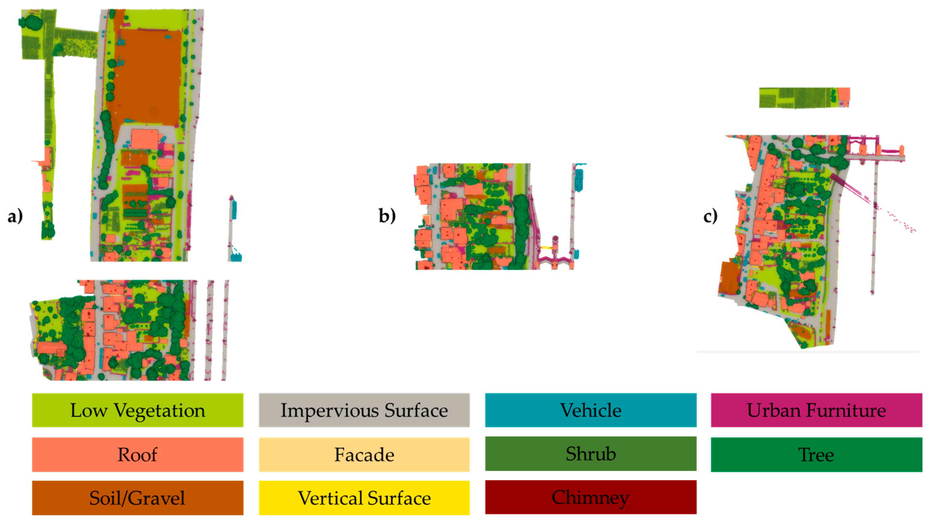
The Hessigheim 3D dataset contains high-density LiDAR data of approximately 800 points/m², enriched with RGB colors. The dataset provides 11 annotated classes: Vehicle, Urban Furniture, Low Vegetation, Impervious Surface, Tree, Roof, Facade, Shrub, Soil/Gravel, Vertical Surface, and Chimney (Figure 3).

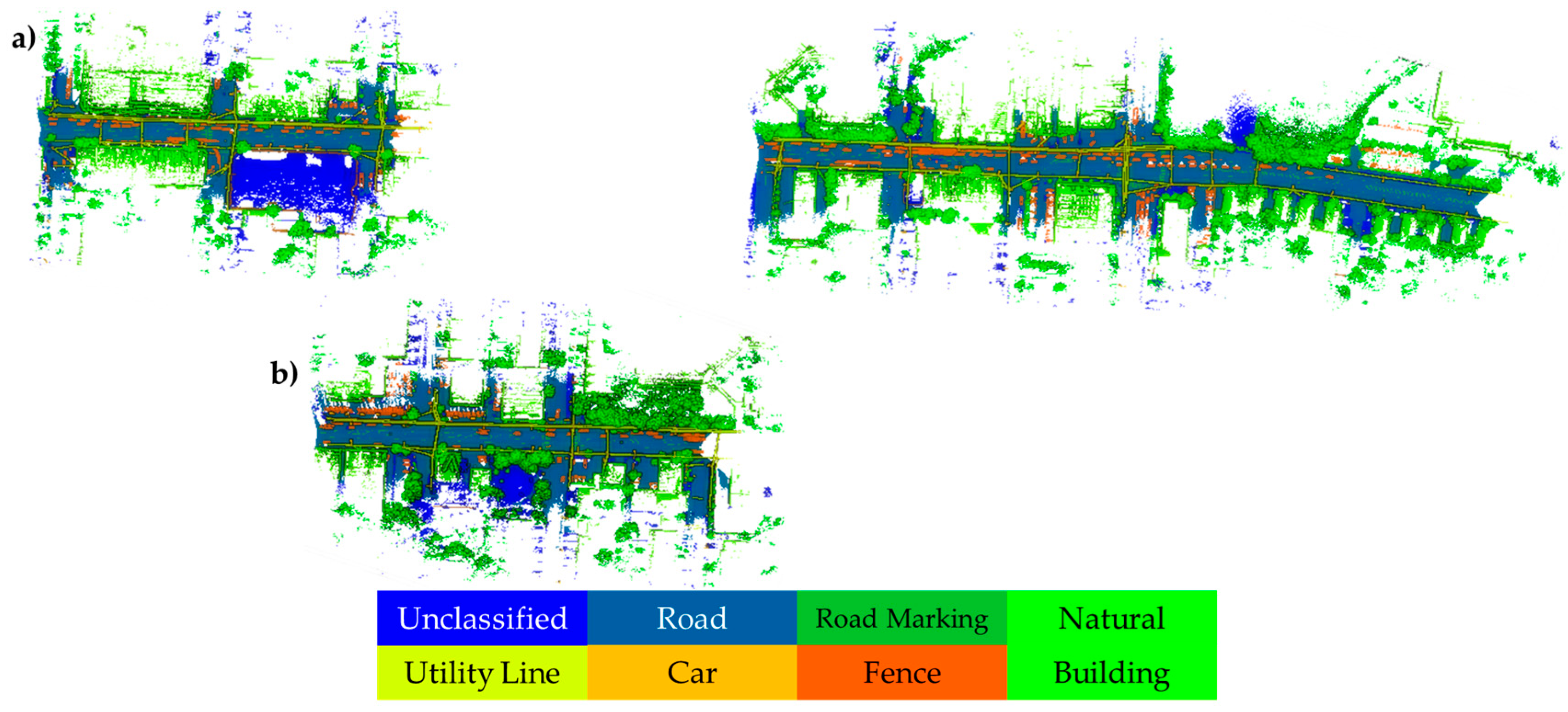
Toronto3D is a large-scale MLS annotated dataset of ca 1000 points/m² depicting Toronto for semantic segmentation tasks on a 1 km urban roadway. The dataset was annotated under 9 classes: Road, Road Marking, Natural, Building, Utility Line, Pole, Car, Fence, and Unclassified (Figure 4).

To avoid precision loss, all training and testing point clouds were translated to a local coordinate system. The training process was configured with a maximum of 200 epochs. The initial learning rate was set to 0.01, with a momentum factor of 0.98. An exponential learning rate decay was applied, where the learning rate was decreased by a factor of 0.1^1/100 per epoch, leading to a 10-fold reduction across 100 epochs. To ensure reproducibility, a fixed random seed (42) was set. All experiments were conducted on a workstation equipped with an Intel Core i9-13900K CPU (Intel, Santa Clara, CA, USA), an NVIDIA RTX 4090 GPU (NVIDIA, Santa Clara, CA, USA) with 24 GB of VRAM, and 64 GB of system memory. To ensure a fair comparison, all experiments on the STPLS3D, Hessigheim3D, and Toronto3D benchmarks were trained using the same hyperparameter settings (

Table 1. Hyperparameters used for training.

Dataset	Hessigheim3D	STPLS3D	Toronto3D
Input Radius (m)	5	18	3
Number of Kernel Points	15	15	15
First Subsampling (m)	0.1	0.5	0.08
Deformable Convolution Radius (m)	6	6	5
Kernel Type	Rigid	Rigid	Rigid
Influence of Each Kernel Point	1.2	1.2	1.0
Aggregation Mode	Sum	Sum	Closest
Minimum Scale	0.8	0.95	0.9
Maximum Scale	1.2	1.05	1.1
Batch Size	6	6	6
Optimizer	SGD	SGD	SGD

) previously adopted for KPConv in the literature [15,62,63].

4.2. Evaluation Metrics

To validate the proposed method, representative evaluation metrics in the utilized benchmark datasets were used to compare with other methods, namely the overall accuracy (OA), the Intersection over Union (IoU), the mean Intersection over Union (mIoU), F1 score, and mean F-1 Score (mF1), with the respective equations being as follows:

$$\mathit{O}\mathit{A}={\displaystyle \frac{\mathit{T}\mathit{P}+\mathit{T}\mathit{N}}{\mathit{T}\mathit{P}+\mathit{T}\mathit{N}+\mathit{F}\mathit{P}+\mathit{F}\mathit{N}}}$$

(7)

$$\mathit{P}\mathit{r}\mathit{e}\mathit{c}\mathit{i}\mathit{s}\mathit{i}\mathit{o}\mathit{n}={\displaystyle \frac{\mathit{T}\mathit{P}}{\mathit{T}\mathit{P}+\mathit{F}\mathit{P}}}$$

(8)

$$\mathit{R}\mathit{e}\mathit{c}\mathit{a}\mathit{l}\mathit{l}={\displaystyle \frac{\mathit{T}\mathit{P}}{\mathit{T}\mathit{P}+\mathit{F}\mathit{N}}}$$

(9)

$$\mathit{F}1\mathit{ }\mathit{S}\mathit{c}\mathit{o}\mathit{r}\mathit{e}={\displaystyle \frac{2·\mathit{P}\mathit{r}\mathit{e}\mathit{c}\mathit{i}\mathit{s}\mathit{i}\mathit{o}\mathit{n}·\mathit{R}\mathit{e}\mathit{c}\mathit{a}\mathit{l}\mathit{l}}{\mathit{P}\mathit{r}\mathit{e}\mathit{c}\mathit{i}\mathit{s}\mathit{i}\mathit{o}\mathit{n}+\mathit{R}\mathit{e}\mathit{c}\mathit{a}\mathit{l}\mathit{l}}}$$

(10)

$$\mathit{I}\mathit{o}\mathit{U}={\displaystyle \frac{\mathit{T}\mathit{P}}{\mathit{T}\mathit{P}+\mathit{F}\mathit{P}+\mathit{F}\mathit{N}}}$$

(11)

where TP represents true-positive samples, TN represents true negatives, FP represents false positives, and FN represents false negatives.

4.3. Performance Comparison

The baseline model results were obtained directly from public leaderboards and studies previously published in the literature, without retraining, to ensure a consistent comparison with benchmark standards. To ensure a fair comparison beyond leaderboard-reported results, we retrained KPConv and Point Transformer (PT) [32] within our own pipeline under identical conditions. Retrained results are denoted as “Ours (retrained)” in the tables to distinguish them from baseline numbers cited directly from prior publications.

Table 2 presents the semantic segmentation results obtained on the STPLS3D dataset for different methods trained using real and synthetic training sets. The results highlight the remarkable performance of our proposed method, LCA (Ours), leveraging synthetic data, which significantly outperforms other methods trained on real data. Specifically, our method achieves a state-of-the-art mean mIoU of 65.32%, representing a substantial improvement of +12.39% compared to VGM, the best-performing method using real data, which obtained a 52.93% mIoU.

Our method exhibits particularly notable performance in classes shown to be traditionally challenging due to their complex geometry and scarcity in terms of point clouds. In the Building class, LCA attains an exceptional IoU of 84.47%, marking an impressive improvement of +21.31% over VGM’s 63.16%. This remarkable improvement underscores the effectiveness of the proposed LCA architecture, which significantly enhances segmentation accuracy for structured, urban environments.

Additionally, LCA demonstrates superior accuracy in detecting smaller and sparser classes such as Light Pole. For the Light Pole class, our method achieves an IoU score of 74.20%, outperforming MinkowskiNet by +8.95% (IoU of 65.25%). On the other hand, in the Fence class, traditionally one of the most challenging classes due to its elongated and fragmented nature, LCA modification attains a notable improvement with an IoU of 14.78%, which is a significant gain of +3.40% compared to KPConv’s 3.40%.

These improvements can be attributed primarily to the LCA model’s effective handling of class imbalance and small-scale objects.

When only synthetic point clouds were included in the training set, the performance increase was not as significant as observed with real training sets. Specifically, our LCA method achieved an average IoU of 51.77%, surpassing MinkowskiNet by only 0.99% and KPConv by approximately 2.5% in terms of mIoU.

However, when both real and synthetic point clouds were included in the training set, LCA achieved a 53.32% mIoU, slightly trailing KPConv’s performance of 53.73% mIoU. Notably, for the Light Pole class, LCA achieved a superior IoU of 58.04%, significantly outperforming KPConv’s 41.30%. To improve performance, the RGB values of both real and synthetic point clouds were standardized using z-score normalization during training. The purpose of this step was to align the color distributions between real and synthetic point clouds, thereby reducing the domain gap. Similar feature standardization strategies have been shown to improve cross-domain generalization in 3D semantic segmentation [64,65]. As a result of this preprocessing, the proposed method achieved an improvement of +5.78% in mIoU and +4.45% in overall accuracy compared to LCA. On a class-wise basis, the gains were particularly notable for Ground (+5.54%), Building (+9.97%), Tree (+10.52%), and Car (+22.51%), whereas a performance decline was observed for the Fence class (−7.05%).

Table 2. Semantic segmentation results on STPLS3D [66] as of August 2025. (N/A: not available). The best results for each class are highlighted in bold.

Training Sets	Methods	mIoU (%)	oAcc (%)	Per-Class IoU (%)
				Ground	Building	Tree	Car	Light Pole	Fence
Real	PT [32]	36.27	54.31	39.95	20.88	62.57	36.13	49.32	8.76
	PT (Ours, retrained)	35.58	53.94	33.50	23.11	64.98	35.11	51.26	5.54
	RandLA-Net [11]	42.33	60.19	46.13	24.23	72.46	53.37	44.82	12.95
	SCF-Net [67]	45.93	75.75	68.77	37.27	65.49	51.50	31.22	21.34
	MinkowskiNet [29]	46.52	70.44	64.22	29.95	61.33	45.96	65.25	12.43
	KPConv [16]	45.22	70.67	60.87	32.13	69.05	53.80	52.08	3.40
	KPConv (Ours, retrained)	43.42	69.21	62.03	29.22	68.44	51.36	48.44	1.07
	VGM [68]	52.93	82.52	77.76	63.16	60.17	39.86	64.13	12.53
	LGFF-Net [69]	49.1	78.8	70.7	55.0	57.3	59.1	38.8	13.6
	PointRAS [70]	47.4	N/A	N/A	N/A	N/A	N/A	N/A	N/A
	DR-Net [71]	48.6	76.2	69.5	37.4	67.0	51.3	54.5	11.9
	LCA (Ours)	65.32	93.08	91.33	84.47	78.63	48.46	74.20	14.78
Synthetic	PT [32]	45.73	86.76	84.12	73.37	60.60	16.96	27.23	12.10
	PT (Ours, retrained)	46.5	87.18	82.79	75.66	57.98	19.22	29.27	14.08
	RandLA-Net [11]	45.03	81.30	76.78	57.74	56.08	28.44	40.36	10.78
	SCF-Net [67]	47.82	82.69	77.51	68.68	56.81	29.87	42.53	11.52
	MinkowskiNet [29]	50.78	87.64	85.23	72.66	64.80	31.31	36.85	13.83
	KPConv [16]	49.16	88.08	85.50	70.65	63.84	28.75	32.97	13.22
	KPConv (Ours, retrained)	45.60	85.89	81.34	64.32	59.13	25.61	34.83	8.36
	LCA (Ours)	51.77	88.29	85.25	77.14	65.47	41.57	31.62	9.54
Real + Synthetic	PT [32]	47.64	84.37	80.19	76.35	57.13	36.35	23.72	12.10
	PT (Ours, retrained)	47.46	83.86	79.35	77.4	56.61	31.14	26.31	13.97
	RandLA-Net [11]	50.53	86.25	82.90	66.59	63.77	33.91	41.84	14.19
	SCF-Net [67]	50.65	83.32	77.80	58.98	64.86	46.37	40.50	15.41
	MinkowskiNet [29]	51.35	84.90	80.86	74.03	59.21	31.72	45.51	16.79
	KPConv [16]	53.73	89.87	87.40	78.51	66.18	39.63	41.30	9.34
	KPConv (Ours, retrained)	47.93	86.71	77.15	71.20	64.73	32.34	37.8	4.34
	PointCT [72]	53.2	N/A	84.1	74.9	62.4	30.4	28.1	15.2
	LCA (Ours)	53.32	87.70	84.53	72.85	65.60	28.87	58.04	10.03
	LCA w/normalization	59.1	92.15	90.07	82.62	76.12	51.38	50.99	3.43

Table 2. Semantic segmentation results on STPLS3D [66] as of August 2025. (N/A: not available). The best results for each class are highlighted in bold.

Training Sets	Methods	mIoU (%)	oAcc (%)	Per-Class IoU (%)
				Ground	Building	Tree	Car	Light Pole	Fence
Real	PT [32]	36.27	54.31	39.95	20.88	62.57	36.13	49.32	8.76
	PT (Ours, retrained)	35.58	53.94	33.50	23.11	64.98	35.11	51.26	5.54
	RandLA-Net [11]	42.33	60.19	46.13	24.23	72.46	53.37	44.82	12.95
	SCF-Net [67]	45.93	75.75	68.77	37.27	65.49	51.50	31.22	21.34
	MinkowskiNet [29]	46.52	70.44	64.22	29.95	61.33	45.96	65.25	12.43
	KPConv [16]	45.22	70.67	60.87	32.13	69.05	53.80	52.08	3.40
	KPConv (Ours, retrained)	43.42	69.21	62.03	29.22	68.44	51.36	48.44	1.07
	VGM [68]	52.93	82.52	77.76	63.16	60.17	39.86	64.13	12.53
	LGFF-Net [69]	49.1	78.8	70.7	55.0	57.3	59.1	38.8	13.6
	PointRAS [70]	47.4	N/A	N/A	N/A	N/A	N/A	N/A	N/A
	DR-Net [71]	48.6	76.2	69.5	37.4	67.0	51.3	54.5	11.9
	LCA (Ours)	65.32	93.08	91.33	84.47	78.63	48.46	74.20	14.78
Synthetic	PT [32]	45.73	86.76	84.12	73.37	60.60	16.96	27.23	12.10
	PT (Ours, retrained)	46.5	87.18	82.79	75.66	57.98	19.22	29.27	14.08
	RandLA-Net [11]	45.03	81.30	76.78	57.74	56.08	28.44	40.36	10.78
	SCF-Net [67]	47.82	82.69	77.51	68.68	56.81	29.87	42.53	11.52
	MinkowskiNet [29]	50.78	87.64	85.23	72.66	64.80	31.31	36.85	13.83
	KPConv [16]	49.16	88.08	85.50	70.65	63.84	28.75	32.97	13.22
	KPConv (Ours, retrained)	45.60	85.89	81.34	64.32	59.13	25.61	34.83	8.36
	LCA (Ours)	51.77	88.29	85.25	77.14	65.47	41.57	31.62	9.54
Real + Synthetic	PT [32]	47.64	84.37	80.19	76.35	57.13	36.35	23.72	12.10
	PT (Ours, retrained)	47.46	83.86	79.35	77.4	56.61	31.14	26.31	13.97
	RandLA-Net [11]	50.53	86.25	82.90	66.59	63.77	33.91	41.84	14.19
	SCF-Net [67]	50.65	83.32	77.80	58.98	64.86	46.37	40.50	15.41
	MinkowskiNet [29]	51.35	84.90	80.86	74.03	59.21	31.72	45.51	16.79
	KPConv [16]	53.73	89.87	87.40	78.51	66.18	39.63	41.30	9.34
	KPConv (Ours, retrained)	47.93	86.71	77.15	71.20	64.73	32.34	37.8	4.34
	PointCT [72]	53.2	N/A	84.1	74.9	62.4	30.4	28.1	15.2
	LCA (Ours)	53.32	87.70	84.53	72.85	65.60	28.87	58.04	10.03
	LCA w/normalization	59.1	92.15	90.07	82.62	76.12	51.38	50.99	3.43

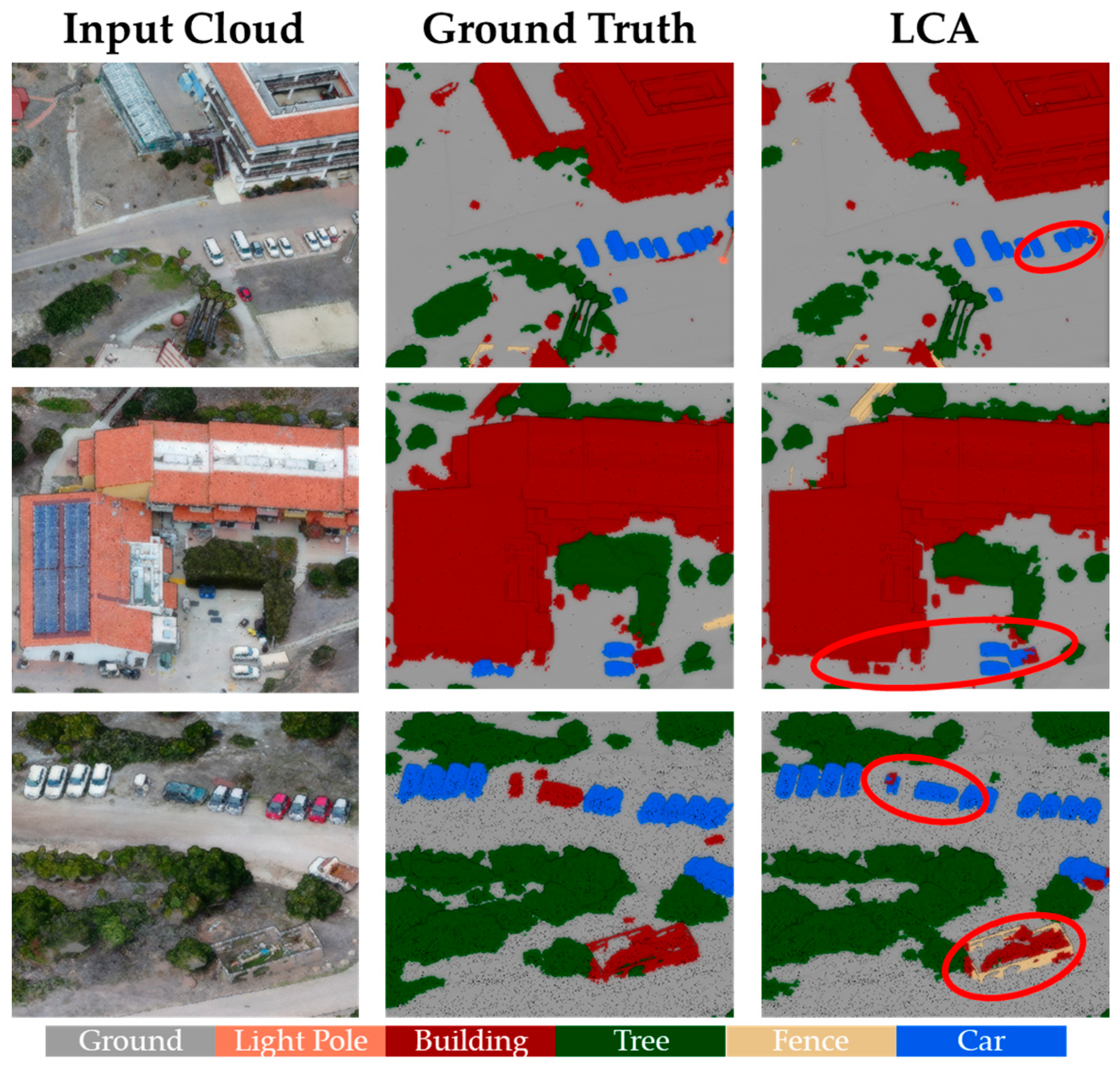
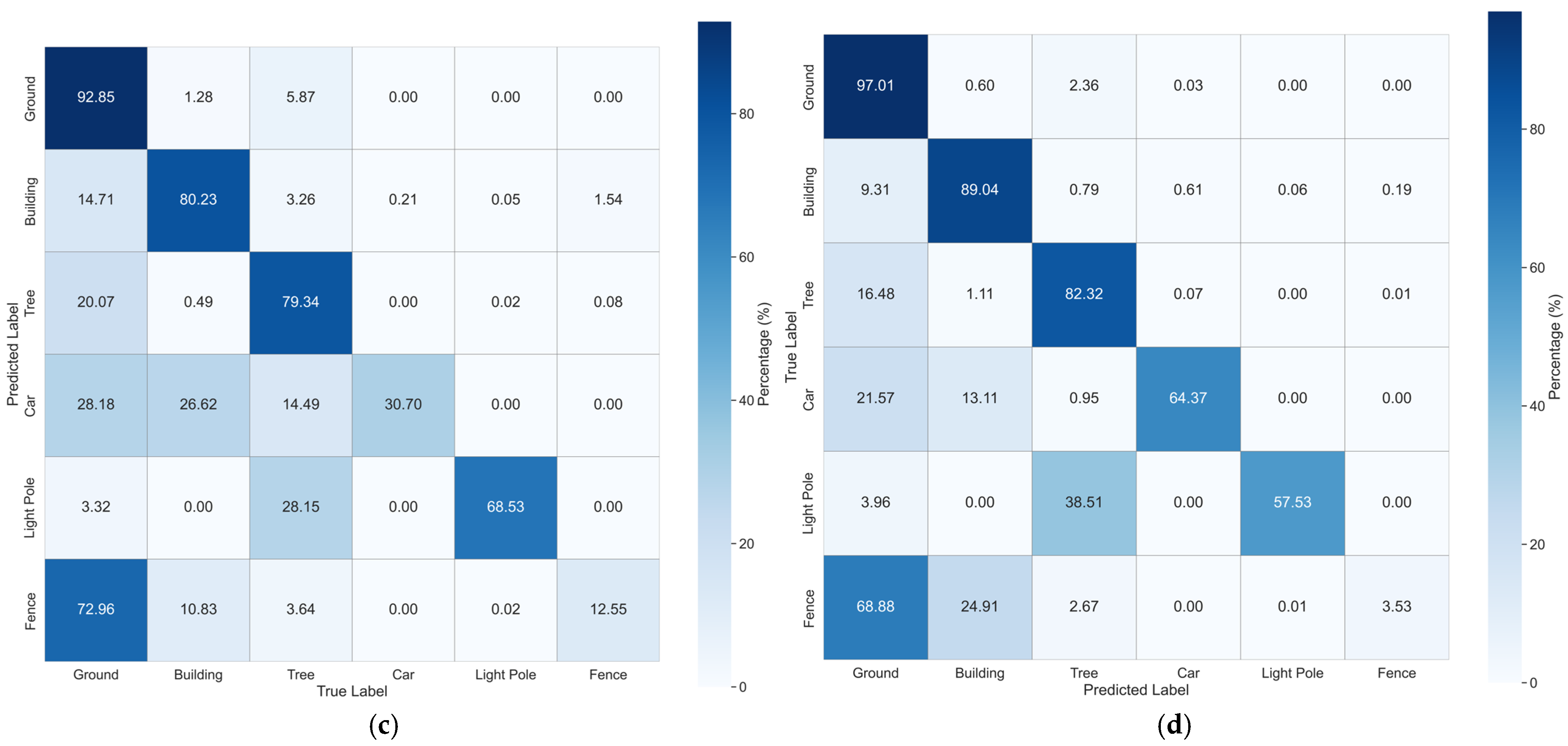
As can be seen from Figure 5, the proposed method yields relatively fewer misclassifications for classes such as Ground, Building, and Tree. However, classes like Fence and Car are more frequently misclassified. In particular, volumetric objects tend to be misclassified as Car–Building and Fence–Building.

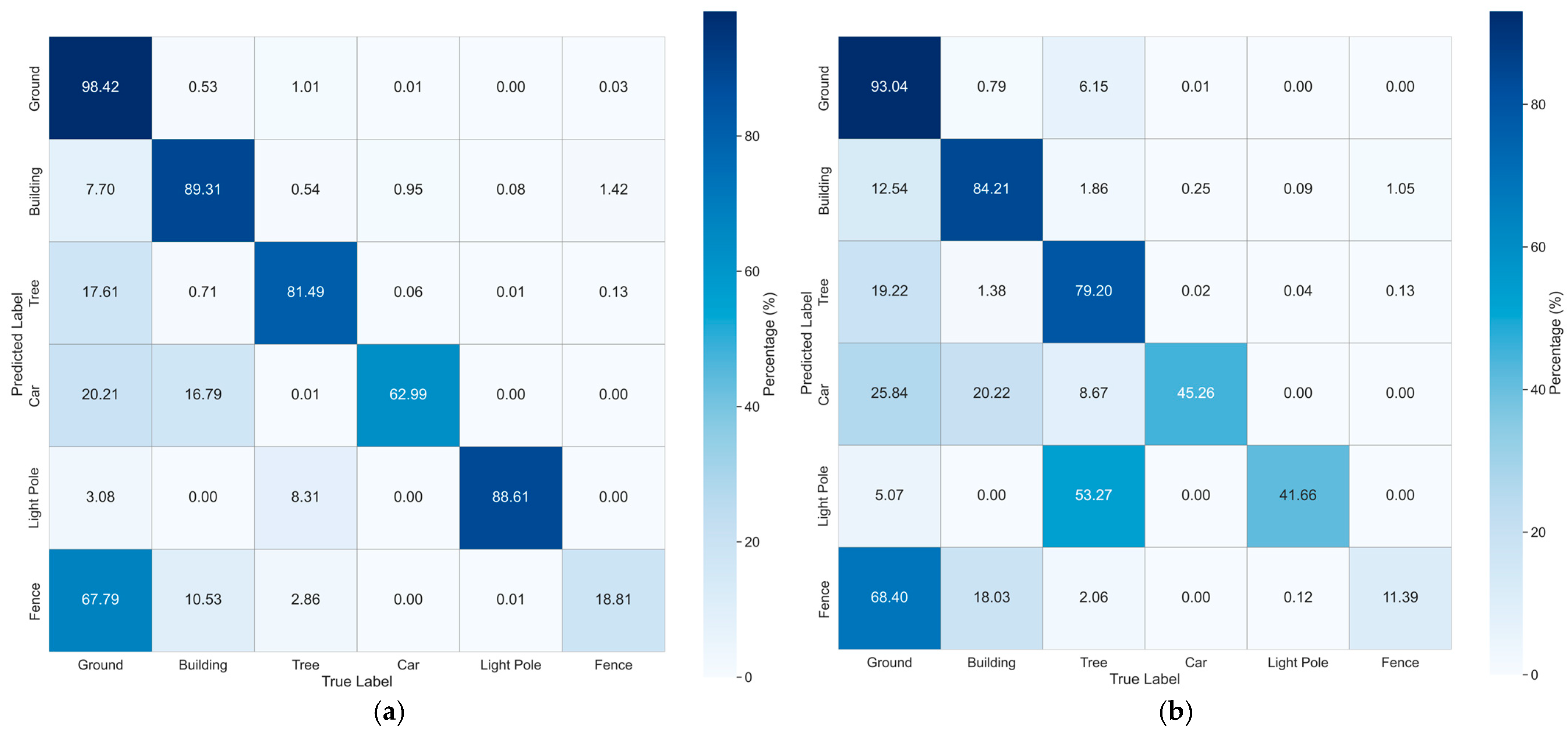
In Figure 6a, the confusion matrix of the model trained on real point clouds and evaluated on the test set reveals notable misclassification patterns, particularly between the Ground–Fence, Ground–Tree, and Car–Building classes. The selection of 0.5 m as the first subsampling parameter in the STPLS3D dataset is likely responsible for the loss of fine-grained details between Ground and Fence, thereby increasing ambiguity. The Ground–Tree confusion, on the other hand, can be attributed to the representation of low vegetation: after resampling, these shrubs are represented by fewer points located close to the ground surface, which limits the model’s ability to separate them from the Ground class. Meanwhile, the misclassification between Car and Building appears to result from relatively small structures in the dataset being annotated as Building, while their volumetric similarity to Car leads to misclassification.

In Figure 6b, the confusion matrix of the LCA model trained on synthetic data and tested on real point clouds is presented. In addition to the previous issues, additional misclassification is observed between Ground and Building, Tree, and Car, as well as between Light Pole and Tree. This can reasonably be explained by the geometric resemblance between Tree and Light Pole objects in the synthetic point cloud, which makes these categories more prone to misclassification.

When training is performed with both real and synthetic point clouds, the problems observed in previous configurations persist; however, a decline in the performance of the Car class and an improvement in the segmentation of the Light Pole class become particularly noticeable.

Table 3. State-of-the-art results (F1 scores) for the Hessigheim3D benchmark [15] as of August 2025. The best results for each class are highlighted in bold.

Method	Low Vegetat.	Impervious Surface	Vehicle	Urban Furniture	Roof	Façade	Shrub	Tree	Soil/Gravel	Vertical Surface	Chimney	mF1	OA
Zhan221112	58.74	22.06	0.32	16.65	57.06	30.02	5.07	69.34	0.11	28.59	2.22	26.38	46.1
PN++ [28]	78.11	72.07	31.78	13.65	73.98	47.79	28.34	71.8	9.65	21.67	4.39	41.2	68.5
Jiabin221114	66.21	18.02	34.18	38.03	72.0	68.99	47.7	78.65	9.84	35.93	8.32	43.44	58.29
Esmoris230208	71.13	55.83	2.73	25.85	93.74	73.28	38.95	93.21	20.68	70.4	49.84	54.15	68.84
Letard230213	68.48	65.4	32.95	42.06	93.61	80.39	43.72	94.17	14.33	72.84	42.45	59.13	66.7
Shi220705 [73]	87.62	85.62	52.4	36.71	95.48	69.3	47.39	94.28	25.08	65.94	38.59	63.49	84.2
Esmoris230207	84.83	81.95	19.45	42.38	94.83	77.77	59.06	94.53	3.55	73.8	69.18	63.76	81.67
Zhan221025	84.33	77.86	58.11	42.32	93.25	65.41	53.53	95.29	23.66	59.85	64.66	65.3	79.69
Sevgen220117	83.86	77.21	66.95	42.64	95.6	80.09	59.53	96.06	25.68	81.51	73.85	71.18	79.25
KPConv [16]	88.57	88.93	82.1	63.89	97.13	85.13	75.24	97.38	42.68	80.87	0.00	72.9	87.69
KPConv (Ours, retr.)	84.43	81.16	79.68	41.80	84.48	78.93	77.34	96.6	34.12	73.57	0.00	66.56	82.41
Grilli220725 [74]	88.91	87.74	74.89	54.27	96.83	78.85	53.21	93.28	43.73	75.89	58.22	73.26	85.33
ifp-RF [60]	90.36	88.55	66.89	51.55	96.06	78.47	67.25	95.91	47.91	59.73	80.65	74.85	87.43
Sevgen220725 [75]	90.88	89.4	77.28	55.76	97.05	81.88	62.06	97.1	23.17	80.27	80.28	75.92	87.59
Qiu230831	91.81	84.74	64.6	52.24	95.04	80.59	68.02	97.35	42.11	74.76	85.1	76.03	86.81
ifp-SCN [60]	92.31	88.14	63.51	57.17	96.86	83.19	68.59	96.98	44.81	78.2	73.61	76.67	88.42
WHU221118	92.9	90.23	78.51	57.89	95.71	80.43	68.46	97.21	62.37	73.08	72.45	79.02	89.75
WHU220322	94.11	91.92	79.42	59.16	97.2	81.86	68.31	96.96	78.94	78.42	84.58	82.81	91.77
PGFormer [54]	89.4	85.2	61.0	48.5	95.7	75.0	61.9	95.4	38.7	76.9	74.1	72.9	85.8
Zhang231204	91.89	90.56	84.12	64.75	97.98	84.21	71.07	97.15	70.66	85.13	84.72	83.84	90.45
PT [74]	90.91	84.5	38.54	43.54	89.06	75.15	58.33	96.18	48.46	64.8	48.86	67.12	84.06
PT (Ours, retrained)	89.15	83.7	41.21	45.69	88.21	78.09	60.11	93.22	48.04	63.54	44.15	66.83	83.89
LCA (Ours)	94.20	93.68	95.38	77.72	98.65	89.48	80.04	97.66	72.87	90.29	88.76	88.98	93.33

illustrates the semantic segmentation results of different methods evaluated on the Hessigheim3D dataset. The results clearly indicate the superior performance of our proposed method, LCA+KPConv, achieving a significant improvement across multiple metrics. Notably, our method attains high per-class mF1 scores, as well as a considerable enhancement in challenging and underrepresented classes, reaching an impressive mF1 score of 88.98%, surpassing the previous best-performing method reported by Zhang231204, which obtained an mF1 of 83.84%.

Of particular interest is the remarkable performance in classes typically problematic due to their small-scale or imbalanced nature. In the Chimney class, our method achieved an mF1 score of 88.76%, an exceptional improvement considering the original KPConv approach scored 0% IoU in this class. This substantial gain underscores the effectiveness of our introduced LCA mechanism in handling small, isolated, or sparsely represented objects, thereby addressing one of the critical limitations of traditional segmentation models.

Furthermore, significant enhancements were observed in classes like Urban Furniture and Vehicle. In the Urban Furniture class, our method improved the mF1 score to 77.72%, marking an increase of +12.97% over Zhang231204’s method (64.75%), indicating the capability of our method to accurately segment scattered and small urban objects. Similarly, in the Vehicle class, we achieved an mF1 score of 95.38%, a considerable improvement (+11.26%) compared to Zhang231204’s performance (84.12%), demonstrating the robustness of our approach against imbalanced class distributions.

These improvements can be attributed primarily to our integration of the LCA mechanism within the KPConv architecture, which effectively preserves local structural details and facilitates improved feature representation for both fine-scale and imbalanced classes.

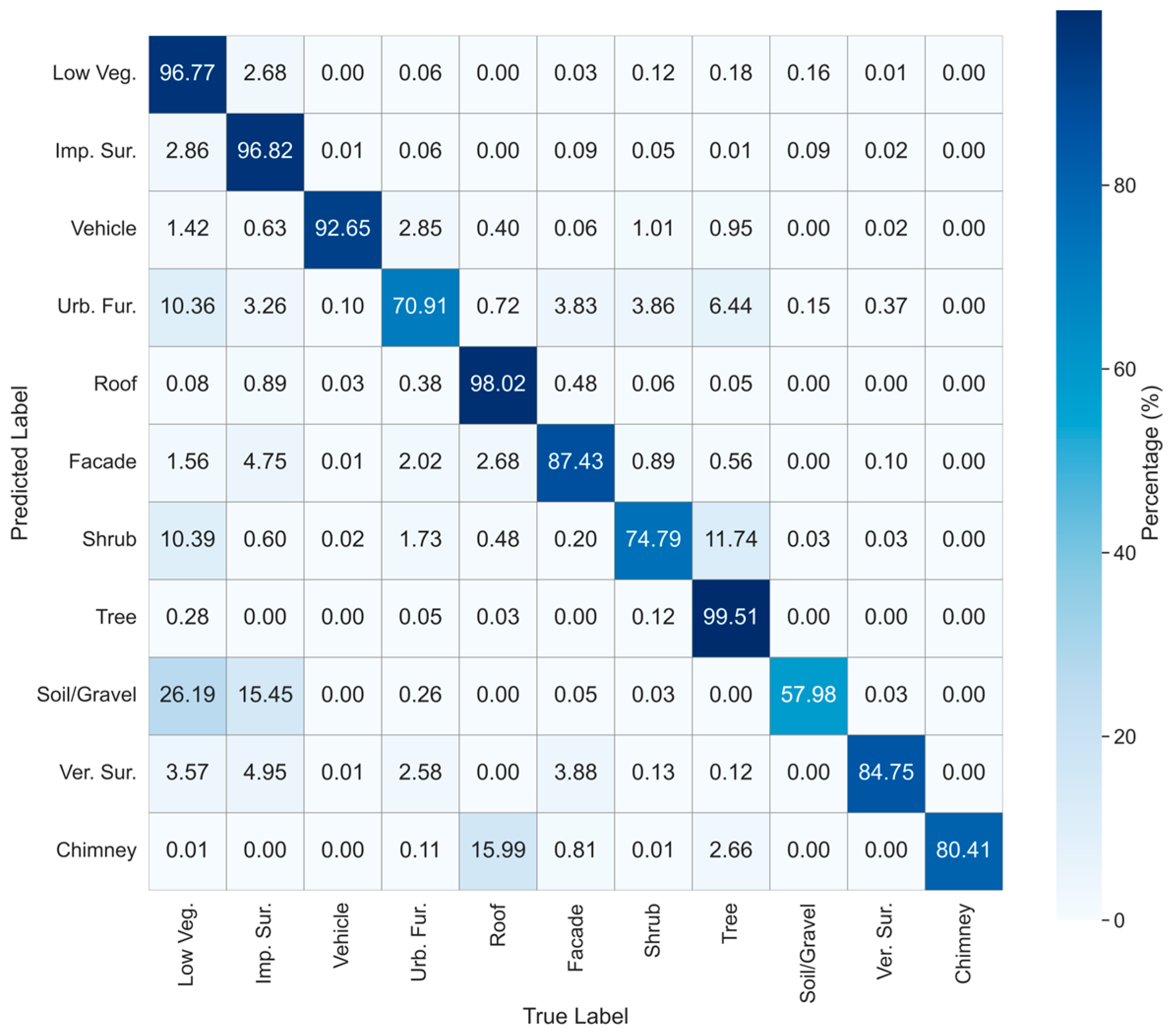
The prediction results presented in Figure 7 indicate that imbalanced and small-scale objects, such as chimneys, vehicles, and urban furniture, have been effectively classified by LCA. Classes like Low Vegetation and Tree have also produced results close to the ground truth. The numerical scores further reveal that the Shrub class, a subset of vegetation, has lower classification accuracy compared to Low Vegetation and Tree. Consequently, it tends to be confused with neighboring classes such as Low Vegetation, Impervious Surface, and Soil/Gravel.

The confusion matrix results of the Hessigheim3D dataset, shown in Figure 8, demonstrate that the most prominent misclassifications occur between the Soil/Gravel, Low Vegetation, and Impervious Surface classes, as well as between Roof–Chimney and Shrub–Tree. Misclassifications among the ground-level classes (Soil/Gravel, Low Vegetation, and Impervious Surface) can be explained by their similar color values and spatial adjacency, which make class boundaries more ambiguous. In addition, since Roof and Chimney objects are naturally located in close proximity on buildings, the results show that distinguishing between these two adjacent classes remains challenging.

According to the results on the Toronto3D dataset (

Table 4. State-of-the-art results (IoU scores) for the Toronto3D benchmark [76] as of August 2025. The best results for each class are highlighted in bold.

Method	OA	mIoU	Road	Road Mark	Natural	Building	Utility Line	Pole	Car	Fence
PointNet++ [28]	92.56	59.47	92.90	0.00	86.13	82.15	60.96	62.81	76.41	14.43
DGCNN [77]	94.24	61.79	93.88	0.00	91.25	80.39	62.40	62.32	88.26	15.81
KPConv [16]	95.39	69.11	94.62	0.06	96.07	91.51	87.68	81.56	85.66	15.72
KPConv (Ours, retr.)	91.07	64.63	92.11	0.00	89.53	85.12	81.28	71.59	83.76	13.59
MS-PCNN [78]	90.03	65.89	93.84	3.83	93.46	82.59	67.80	71.95	91.12	22.50
TGNet [79]	94.08	61.34	93.54	0.00	90.83	81.57	65.26	62.98	88.73	7.85
MS-TGNet [61]	95.71	70.50	94.41	17.19	95.72	88.83	76.01	73.97	94.24	23.64
DiffConv [80]	-	76.73	83.31	51.06	69.04	79.55	80.48	84.41	76.19	89.83
EyeNet [81]	94.63	81.13	96.98	65.02	97.83	93.51	86.77	84.86	94.02	30.01
DCTNet [82]	-	81.84	82.77	59.53	85.51	86.47	81.79	84.03	79.55	96.21
RandLA-Net [11]	94.37	81.77	96.69	64.21	96.92	94.24	88.06	77.84	93.37	42.86
Rim et al. [83]	83.60	71.03	92.84	27.43	89.90	95.27	85.59	74.50	44.41	58.30
MappingConvSeg [84]	94.72	82.89	97.15	67.87	97.55	93.75	86.88	82.12	93.72	44.11
ResDLPS-Net [85]	96.49	80.27	95.82	59.80	96.10	90.96	86.82	79.95	89.41	43.31
LACV-Net [86]	97.4	82.7	97.1	66.9	97.3	93.0	87.3	83.4	93.4	43.1
PGFormer [54]	96.5	81.1	95.9	50.5	95.9	91.5	79.7	72.8	93.0	39.9
LGFF-Net	97.2	81.4	96.9	65.5	96.1	92.7	86.0	78.8	93.6	41.4
PT [32]	96.8	79.9	96.7	64.6	95.9	91.0	87.6	79.0	87.5	36.9
PT (Ours, retrained)	93.11	74.69	84.23	59.14	87.01	90.18	81.92	74.43	82.17	38.46
Han et al. [87]	93.60	70.80	92.20	53.80	92.80	86.00	72.20	72.50	75.70	21.20
LCA (Ours)	96.62	84.06	95.99	57.66	96.86	95.76	88.14	88.07	96.06	53.91

), the proposed method achieved the highest mIoU score of 84.06%. In terms of OA, it obtained a value of 96.62%, ranking second only to LACV-Net, which achieved a value of 97.4%. A noteworthy observation is that, while LCA attains the highest mIoU score overall, it achieves the best per-class performance only for the Building, Pole, and Car categories. For other categories, the leading results are achieved by different methods: MappingConvSeg achieves the best performance for Road (97.15% IoU) and Road Marking (67.87% IoU), EyeNet performs best on the Natural class (97.83% IoU), LACV-Net achieves the highest IoU for Utility Line (88.2%), and DiffConv provides the top performance for Fence (89.83% IoU).

Compared to the original KPConv, integrating the proposed LCA block yields an approximate 15% improvement in mIoU. Furthermore, the IoU scores for the Road Marking and Fence classes, which were only 0.06% and 15.72% with KPConv, are significantly enhanced to 57.66% and 53.91%, respectively, when using the LCA-based approach.

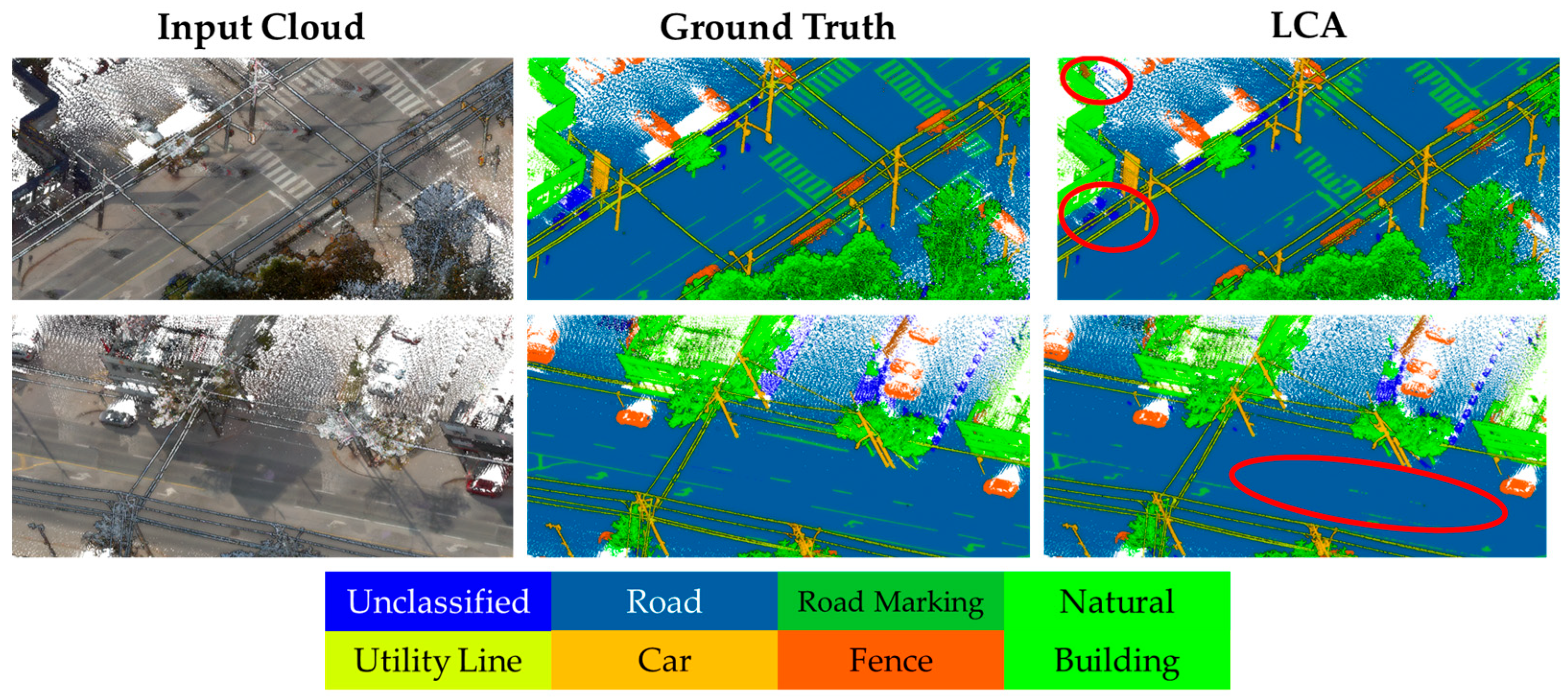
Figure 9 presents the Toronto3D prediction results obtained with the LCA approach. While some misclassifications are observed between the Road and Road Marking classes, certain points belonging to the Building class are incorrectly assigned as Fence. Additionally, objects that should remain Unclassified are occasionally misclassified as trees within the Natural class or as Utility Line. Nevertheless, both visual and numerical results confirm that objects such as Road, Natural, Building, and Car are predominantly classified correctly.

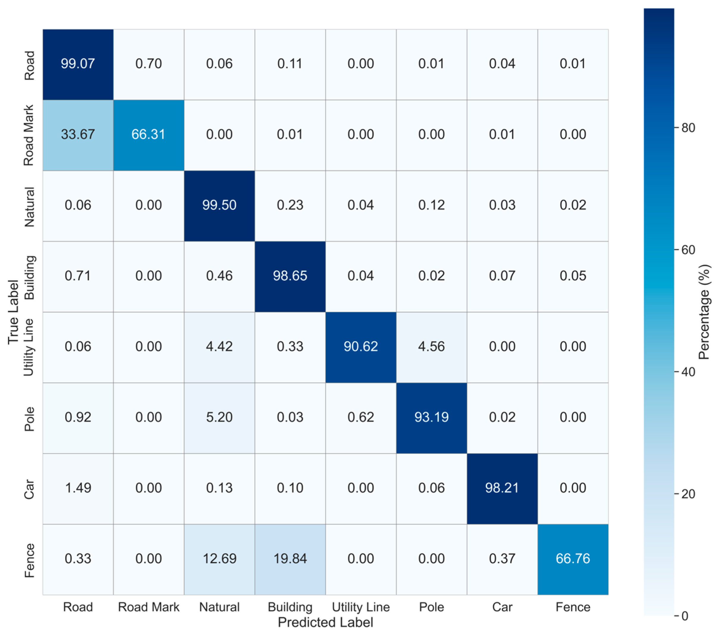
The detailed results for the Toronto3D dataset in Figure 10 reveal that the most common misclassifications occur between the Road and Road Mark classes. As on the STPLS3D and Hessigheim3D datasets, these results validate the difficulty in distinguishing adjacent objects that lie on the same surface. Additional misclassifications are observed between the Fence–Building and Natural–Fence classes, which can be attributed to their similar vertical geometric structures in the MLS-based Toronto3D dataset, leading to a higher degree of confusion.

4.4. Ablation Study

The LCA block, proposed as an extension to the baseline KPConv, substantially enhances the network’s performance, as evidenced by the results summarized in

Table 5. Comparison of baseline KPConv and LCA-enhanced KPConv across benchmarks. The best results for each dataset are highlighted in bold.

Dataset	Method	OA	mIoU	mF1
STPLS3D Real	KPConv	70.67	45.22	-
	KPConv (Ours, retrained)	69.21	43.42
	LCA (Ours)	93.08	65.32	-
STPLS3D Synthetic	KPConv	88.08	49.16	-
	KPConv (Ours, retrained)	85.89	45.60
	LCA (Ours)	88.29	51.77	-
STPLS3D Real+Synthetic	KPConv	88.08	53.73	-
	KPConv (Ours, retrained)	86.71	47.93
	LCA (Ours)	88.29	53.32	-
	LCA w/normalization	90.60	57.55
Hessigheim3D	KPConv	87.69	-	72.9
	KPConv (Ours, retrained)	82.41		66.56
	LCA (Ours)	93.33	-	88.98
Toronto3D	KPConv	95.39	69.11	-
	KPConv (Ours, retrained)	91.07	64.63
	LCA (Ours)	96.62	84.06	-

. On the STPLS3D dataset, when trained with real point clouds, the mIoU score improved by 20.1%. However, the addition of synthetic data resulted in only a 2% increase, and in the combined real and synthetic training scenario, the LCA block yielded slightly lower performance than KPConv.

On the Hessigheim3D and Toronto3D datasets, the incorporation of LCA led to an improvement in mF1 and mIoU scores of 15%. These experiments clearly demonstrate that the proposed LCA block significantly enhances the performance of the KPConv architecture.

As can be seen in

Table 6. Effect of KPConv parameters on STPLS3D benchmark’s real+synthetic training configuration. The best classification results are highlighted in bold.

LCA	Input Radius (m)	Number of Kernel Points	D_Hidden	OA	mIoU
w/o norm.	15	18	${in}_{dim}/4$	88.29	53.32
	15	15	${in}_{dim}/4$	87.06	53.16
	15	21	${in}_{dim}/4$	88.40	53.68
	18	18	${in}_{dim}/4$	89.49	54.26
	18	15	${in}_{dim}/4$	89.34	53.97
	18	21	${in}_{dim}/4$	90.11	54.49
	12	18	${in}_{dim}/4$	85.20	50.09
	12	15	${in}_{dim}/4$	84.72	49.82
	12	21	${in}_{dim}/4$	85.84	50.23
	15	18	${in}_{dim}/2$	90.43	55.17
	15	15	${in}_{dim}/2$	89.11	54.66
	15	21	${in}_{dim}/2$	91.53	55.38
	18	18	${in}_{dim}/2$	91.61	55.41
	18	15	${in}_{dim}/2$	89.50	54.27
	18	21	${in}_{dim}/2$	92.84	57.74
	12	18	${in}_{dim}/2$	87.39	53.29
	12	15	${in}_{dim}/2$	87.30	53.11
	12	21	${in}_{dim}/2$	87.51	53.34
w/norm.	15	18	${in}_{dim}/4$	90.60	57.55
	15	15	${in}_{dim}/4$	89.13	56.1
	15	21	${in}_{dim}/4$	91.16	57.93
	18	18	${in}_{dim}/4$	91.97	58.36
	18	15	${in}_{dim}/4$	90.13	56.72
	18	21	${in}_{dim}/4$	92.44	59.06
	12	18	${in}_{dim}/4$	87.14	54.33
	12	15	${in}_{dim}/4$	85.66	53.09
	12	21	${in}_{dim}/4$	88.31	54.79
	15	18	${in}_{dim}/2$	91.67	58.16
	15	15	${in}_{dim}/2$	90.32	56.83
	15	21	${in}_{dim}/2$	92.08	58.84
	18	18	${in}_{dim}/2$	93.15	59.77
	18	15	${in}_{dim}/2$	92.56	58.13
	18	21	${in}_{dim}/2$	93.47	59.96
	12	18	${in}_{dim}/2$	89.04	56.0
	12	15	${in}_{dim}/2$	88.73	54.94
	12	21	${in}_{dim}/2$	89.51	55.58

, we conducted a controlled ablation study on the input neighborhood radius r, the number of kernel points K, and the $d_{hidden}$ in LCA under real+synthetic training on STPLS3D. Experiments were repeated without and with feature normalization. Without normalization, three patterns are clear. First, the neighborhood radius is the principal driver of performance. For fixed K and $d_{hidden}$, r from 12 to 18 yields consistent gains in both OA and mIoU. For example, with K = 21 $d_{hidden}={in}_{dim}/4$, mIoU improves from 50.23% (12 m) to 53.68% (15 m) to 54.49% (18 m), with OA changing from 85.84% to 88.40% to 90.11%. This trend indicates that, in mixed-domain training, enlarging the effective receptive field helps the model exploit more stable geometric context and offsets cross-domain variability in local appearance. Second, increasing the number of kernel points provides incremental but smaller benefits than enlarging r. At r = 15 and $d_{hidden}={in}_{dim}/4$, moving from K = 15 → 18 → 21 changes mIoU only modestly (53.16% → 53.32% → 53.68%), and the same is true for OA (87.06% → 88.29% → 88.40%). A similar pattern holds at r=18 (e.g., mIoU 53.97% → 54.26% → 54.49%; OA 89.34% → 89.49% → 90.11%). These results suggest that denser kernel sampling refines local aggregation but is secondary to the spatial context controlled by r. Third, model capacity interacts positively with both r and K. Widening from $d_{hidden}={in}_{dim}/4$ to $d_{hidden}={in}_{dim}/2$ consistently amplifies the gains when r and K are large. At r = 18, K = 21 leads to performance improvements of from 54.49% mIoU and 90.11% OA (${in}_{dim}/4$) to 57.74%/92.84% (${in}_{dim}/2$), i.e., +3.25 mIoU and +2.73 OA. Overall, the best unnormalized configuration in our sweep is r = 18 m, K = 21, $d_{hidden}={in}_{dim}/2$ at 57.74% mIoU and 92.84% OA, while the weakest is r = 12 m, K = 15, $d_{hidden}={in}_{dim}/4$ at 49.82%/84.72%. The spread (+7.9 mIoU, +8.1 OA) underscores the sensitivity of the mixed real+synthetic setting to hyperparameter choice and explains why under-tuned, unnormalized models can underperform a standard KPConv baseline.

With feature normalization enabled, the ordering of configurations remains the same, and the optimum again occurs at the high-context, higher-capacity setting—r = 18 m, K = 21, $d_{hidden}={in}_{dim}/2$—resulting in a further improvement to 59.96% mIoU/93.47% OA. This gain supports the hypothesis that normalization mitigates cross-domain scale/contrast shifts, while r, K, and $d_{hidden}$ determine how effectively the network capitalizes on that stabilization.

In summary, the ablation aligns with the study’s aim of characterizing robustness in real+synthetic training: (i) prioritize r at the upper end permitted by the point cloud resolution (here, 18 m), (ii) use a moderate-to-high kernel-point capability (≈21) for diminishing-return refinements, and (iii) allocate sufficient $d_{hidden}\ge {in}_{dim}/2$ to leverage the expanded context—ideally in conjunction with feature normalization.

Compared to KPConv and Point Transformer, LCA marginally increases FLOPs by +6.2% and +36.6% while introducing a larger parameter footprint, +64.8% and +16.6%, respectively. (

Table 7. Comparison of network complexity.

Method	FLOPs	Parameters (M)	Maximum VRAM Usage (GB)	Latency (Second/Epoch)
				STPLS3D	Hessigheim3D	Toronto3D
KPConv	6.5	14.93	~6.7	7.43	10.24	3.87
Point Transformer	5.05	21.1	~12.4	12.27	18.40	6.28
LCA (Ours)	6.9	24.61	~8.9	9.69	13.04	5.84

). Despite the modest compute overhead, per-epoch latency rises by 27–51% across datasets, indicating memory-/bandwidth-bound costs due to per-neighborhood attention and softmax operations. By contrast, Point Transformer carries ~30M parameters—approximately +101% over the KPConv baseline (14.93M) and +22% over LCA (24.61M). In terms of memory, LCA’s maximum VRAM usage (8.9 GB) exceeds KPConv’s (6.7 GB) yet remains well below Point Transformer’s (12.4 GB)—about +33% vs. KPConv and −28% vs. Point Transformer.

5. Discussion

Experimental results have demonstrated that the proposed LCA block achieves the highest classification accuracy across three large-scale outdoor 3D datasets. By leveraging the strong local geometric features extracted through KPConv’s kernel point weighting, the LCA block enhances local contextual representation via point-wise attention. This ability to capture local context provides automatic adaptability to point clouds with varying densities and structural complexities. Consequently, the integration of LCA has been shown to improve classification accuracy for challenging classes such as Fence, Pole, and Chimney.

The addition of the LCA block into KPConv has led to superior results on the STPLS3D, Hessigheim3D, and Toronto3D datasets, outperforming strong baseline models such as RandLA-Net, Point Transformer, and MinkowskiNet.

However, on the STPLS3D dataset, incorporating synthetic point clouds into the training set did not yield the expected performance gain, resulting in outcomes comparable to other methods. This can be attributed to the inherent characteristics of synthetic data, which typically provide noise-free, smooth-surfaced, and optimally sampled examples. In contrast, real-world data are often noisy, incomplete, or irregular. Attention-based mechanisms like LCA are inherently sensitive to local context; thus, the artificial homogeneity of synthetic data negatively affects the learning of neighborhood relationships, ultimately reducing generalization capability. Nevertheless, applying Z-score standardization to the input features enhanced model performance, mirroring the gains typically observed with statistics-based preprocessing in domain adaptation [51]. In the mixed real–synthetic training configuration examined here, LCA’s performance is governed not only by architectural choice but also by hyperparameterization. Our ablation indicates that the input neighborhood radius is the primary determinant of accuracy: enlarging the radius systematically improves OA and mIoU, whereas increases in kernel-point count and hidden width yield secondary, diminishing-return gains. This pattern is consistent with prior evidence [88], which similarly emphasizes that selecting baseline KPConv’s effective convolutional support (i.e., the receptive field governed by radius) is decisive for segmentation quality.

When examining the scores in Table 2, the discrepancies between the reported results and our retrained counterparts on the STPLS3D dataset are relatively modest—approximately within 2% mIoU for both Point Transformer and KPConv in the real and synthetic training configurations. However, a more pronounced gap emerges in the real+synthetic setting, where the reported KPConv achieves an average of 53.73% mIoU, whereas our retrained model reaches only 47.93% mIoU. Comparable deviations were observed on the Hessigheim3D (Table 3) and Toronto3D (Table 4) datasets, where retrained models underperformed compared to the reported results by approximately 4–7% mIoU. Such discrepancies, despite carefully maintaining consistency in training parameters, have also been highlighted in the literature [89] as a consequence of subtle differences in experimental conditions, preprocessing pipelines, or implementation details.

Confusion matrix analysis across the three benchmark datasets points out that the most recurrent misclassifications arise from adjacent or geometrically similar categories. On STPLS3D, the confusion between Ground–Fence, Ground–Tree, and Car–Building is largely due to subsampling-induced loss of fine details and the volumetric similarity of small buildings to cars. In the synthetic-to-real setting, errors extend to Ground–Building and Tree–Light Pole, reflecting geometric resemblance in synthetic objects. For Hessigheim3D, misclassifications mainly occur among Soil/Gravel–Low Vegetation–Impervious Surface, and Roof–Chimney, where adjacency and spectral similarity hinder boundary delineation. Finally, Toronto3D results reveal dominant confusion between Road–Road Mark, with additional errors such as Fence–Building and Natural–Fence due to vertical structural similarities in MLS data.

To address these issues, several targeted improvements may be considered. First, the integration of boundary-aware loss functions [90,91] could explicitly penalize misclassifications near object borders and improve boundary delineation. Second, multi-scale context aggregation [92] would allow the network to better capture both fine-grained local cues and global spatial context, which is particularly relevant for distinguishing adjacent classes on the same surface (e.g., Road–Road Mark). Third, incorporating shape priors or structural constraints [93] may help disambiguate volumetrically similar classes such as Car–Building or Fence–Building. Together, these strategies highlight promising directions for mitigating recurrent misclassifications while complementing the lightweight, single-block design of the proposed LCA.

6. Conclusions

This research proposes a new approach for incorporating features of KPConv with respect to the Local Context Attention (LCA) mechanism for 3D point cloud semantic segmentation. As of August 2025, the proposed methodology achieves the highest classification performance on the STPLS3D, Hessigheim3D, and Toronto3D benchmarks. The LCA source codes, trained models, and the generated point clouds are publicly available at https://github.com/onurcbayrak/LCA-KPConv (accessed on 5 August 2025).

Overall, this contribution comes up with a promising solution for semantic segmentation of imbalanced classes and small urban objects by leveraging the power of kernel points and attention mechanisms to emphasize the importance of local feature descriptors.

Practically, our findings for mixed real-synthetic point clouds imply that a principled radius selection—paired with a moderate kernel-point budget—is necessary to realize the benefits of LCA and to avoid underperformance relative to baselines, particularly when features are left unnormalized. We therefore recommend that future comparisons report and justify radius choices and include sensitivity analyses over radius and kernel-point count to ensure fairness and reproducibility.

Furthermore, LCA can potentially be adapted for any 3D semantic segmentation network. In future work, we plan to enhance the performance of LCA trained with synthetic data by employing techniques such as domain adaptation, feature standardization, joint fine-tuning, hybrid attention, etc. These approaches aim to mitigate the negative impact of local context discrepancies introduced by synthetic data.

References

1. Liamis, T.; Mimis, A. Establishing Semantic 3D City Models by GRextADE: The Case of the Greece. J. Geovis. Spat. Anal. 2022, 6, 15. [Google Scholar] [CrossRef]
2. Iman Zolanvari, S.M.; Ruano, S.; Rana, A.; Cummins, A.; Da Silva, R.E.; Rahbar, M.; Smolic, A. DublinCity: Annotated LiDAR Point Cloud and Its Applications. In Proceedings of the 30th British Machine Vision Conference 2019, BMVC 2019, Cardiff, UK, 9–12 September 2019. [Google Scholar]
3. Shen, Z.; He, Y.; Du, X.; Yu, J.; Wang, H.; Wang, Y. YCANet: Target Detection for Complex Traffic Scenes Based on Camera-LiDAR Fusion. IEEE Sens. J. 2024, 24, 8379–8389. [Google Scholar] [CrossRef]
4. Abbas, Y.; Alarfaj, A.A.; Alabdulqader, E.A.; Algarni, A.; Jalal, A.; Liu, H. Drone-Based Public Surveillance Using 3D Point Clouds and Neuro-Fuzzy Classifier. Comput. Mater. Contin. 2025, 82, 4759–4776. [Google Scholar] [CrossRef]
5. Bai, Q.; Lindenbergh, R.C.; Vijverberg, J.; Guelen, J.A.P. Road Type Classification of MLS Point Clouds Using Deep Learning. Int. Arch. Photogramm. Remote Sens. Spat. Inf. Sci.–ISPRS Arch. 2021, 43, 115–122. [Google Scholar] [CrossRef]
6. Yu, W.; Shu, J.; Yang, Z.; Ding, H.; Zeng, W.; Bai, Y. Deep Learning-Based Pipe Segmentation and Geometric Reconstruction from Poorly Scanned Point Clouds Using BIM-Driven Data Alignment. Autom. Constr. 2025, 173, 106071. [Google Scholar] [CrossRef]
7. Breiman, L. Random Forests. Mach. Learn. 2001, 45, 5–32. [Google Scholar] [CrossRef]
8. Ke, G.; Meng, Q.; Finley, T.; Wang, T.; Chen, W.; Ma, W.; Ye, Q.; Liu, T.-Y. LightGBM: A Highly Efficient Gradient Boosting Decision Tree. Adv. Neural Inf. Process Syst. 2017, 30, 52. [Google Scholar]
9. Chen, T.; Guestrin, C. XGBoost: A Scalable Tree Boosting System. In Proceedings of the 22nd ACM SIGKDD International Conference on Knowledge Discovery and Data Mining, San Francisco, CA, USA, 13–17 August 2016; pp. 785–794. [Google Scholar] [CrossRef]
10. Weinmann, M.; Jutzi, B.; Hinz, S.; Mallet, C. Semantic Point Cloud Interpretation Based on Optimal Neighborhoods, Relevant Features and Efficient Classifiers. ISPRS J. Photogramm. Remote Sens. 2015, 105, 286–304. [Google Scholar] [CrossRef]
11. Hu, Q.; Yang, B.; Xie, L.; Rosa, S.; Guo, Y.; Wang, Z.; Trigoni, N.; Markham, A. Randla-Net: Efficient Semantic Segmentation of Large-Scale Point Clouds. In Proceedings of the IEEE Computer Society Conference on Computer Vision and Pattern Recognition, Seattle, WA, USA, 13–19 June 2020. [Google Scholar]
12. Hu, Q.; Yang, B.; Khalid, S.; Xiao, W.; Trigoni, N.; Markham, A. Towards Semantic Segmentation of Urban-Scale 3D Point Clouds: A Dataset, Benchmarks and Challenges. In Proceedings of the IEEE Computer Society Conference on Computer Vision and Pattern Recognition, Nashville, TN, USA, 20–25 June 2021. [Google Scholar]
13. Mao, Y.; Chen, K.; Diao, W.; Sun, X.; Lu, X.; Fu, K.; Weinmann, M. Beyond Single Receptive Field: A Receptive Field Fusion-and-Stratification Network for Airborne Laser Scanning Point Cloud Classification. ISPRS J. Photogramm. Remote Sens. 2022, 188, 45–61. [Google Scholar] [CrossRef]
14. Ren, P.; Xia, Q. Classification Method for Imbalanced LiDAR Point Cloud Based on Stack Autoencoder. Electron. Res. Arch. 2023, 31, 3453–3470. [Google Scholar] [CrossRef]
15. Benchmark on High Density Aerial Image Matching. Available online: https://ifpwww.ifp.uni-stuttgart.de/benchmark/hessigheim/results.aspx (accessed on 4 August 2025).
16. Thomas, H.; Qi, C.R.; Deschaud, J.E.; Marcotegui, B.; Goulette, F.; Guibas, L. KPConv: Flexible and Deformable Convolution for Point Clouds. In Proceedings of the IEEE International Conference on Computer Vision, Seoul, Republic of Korea, 27 October–2 November 2019. [Google Scholar]
17. Zhang, H.; Wang, C.; Tian, S.; Lu, B.; Zhang, L.; Ning, X.; Bai, X. Deep Learning-Based 3D Point Cloud Classification: A Systematic Survey and Outlook. Displays 2023, 79, 102456. [Google Scholar] [CrossRef]
18. Su, H.; Maji, S.; Kalogerakis, E.; Learned-Miller, E. Multi-View Convolutional Neural Networks for 3D Shape Recognition. In Proceedings of the IEEE International Conference on Computer Vision (ICCV), Santiago, Chile, 7–13 December 2015. [Google Scholar]
19. Yu, T.; Meng, J.; Yuan, J. Multi-View Harmonized Bilinear Network for 3D Object Recognition. In Proceedings of the Proceedings of the IEEE Computer Society Conference on Computer Vision and Pattern Recognition, Salt Lake City, UT, USA, 18–23 June 2018. [Google Scholar]
20. Ren, H.; Wang, J.; Yang, M.; Velipasalar, S. PointOfView: A Multi-Modal Network for Few-Shot 3D Point Cloud Classification Fusing Point and Multi-View Image Features. In Proceedings of the IEEE/CVF Conference on Computer Vision and Pattern Recognition (CVPR) Workshops, Seattle, WA, USA, 17–18 June 2024; pp. 784–793. [Google Scholar]
21. Kim, Y.; Cho, B.; Ryoo, S.; Lee, S. Multi-View Structural Convolution Network for Domain-Invariant Point Cloud Recognition of Autonomous Vehicles. arXiv 2025, arXiv:2501.16289. [Google Scholar]
22. Guo, Y.; Wang, H.; Hu, Q.; Liu, H.; Liu, L.; Bennamoun, M. Deep Learning for 3D Point Clouds: A Survey. IEEE Trans. Pattern Anal. Mach. Intell. 2021, 43, 4338–4364. [Google Scholar] [CrossRef] [PubMed]
23. Maturana, D.; Scherer, S. VoxNet: A 3D Convolutional Neural Network for Real-Time Object Recognition. In Proceedings of the IEEE International Conference on Intelligent Robots and Systems, Hamburg, Germany, 28 September–2 October 2015. [Google Scholar]
24. Lin, Y.; Wang, C.; Zhai, D.; Li, W.; Li, J. Toward Better Boundary Preserved Supervoxel Segmentation for 3D Point Clouds. ISPRS J. Photogramm. Remote Sens. 2018, 143, 39–47. [Google Scholar] [CrossRef]
25. Zhang, K.; Cai, R.; Wu, X.; Zhao, J.; Qin, P. IBALR3D: ImBalanced-Aware Long-Range 3D Semantic Segmentation. Comput. Sci. Math. Forum 2024, 9, 6. [Google Scholar]
26. Bie, L.; Xiao, G.; Li, Y.; Gao, Y. HyperG-PS: Voxel Correlation Modeling via Hypergraph for LiDAR Panoptic Segmentation. Fundam. Res. 2025; in press. [Google Scholar] [CrossRef]
27. Qi, C.R.; Su, H.; Mo, K.; Guibas, L.J. PointNet: Deep Learning on Point Sets for 3D Classification and Segmentation. In Proceedings of the 30th IEEE Conference on Computer Vision and Pattern Recognition, CVPR 2017, Honolulu, HI, USA, 22–25 July 2017. [Google Scholar]
28. Qi, C.R.; Yi, L.; Su, H.; Guibas, L.J. PointNet++: Deep Hierarchical Feature Learning on Point Sets in a Metric Space. Adv. Neural Inf. Process. Syst. 2017, 30. [Google Scholar]
29. Choy, C.; Gwak, J.; Savarese, S. 4D Spatio-Temporal Convnets: Minkowski Convolutional Neural Networks. In Proceedings of the IEEE Computer Society Conference on Computer Vision and Pattern Recognition, Long Beach, CA, USA, 15–20 June 2019. [Google Scholar]
30. Zhang, H.; Wang, C.; Yu, L.; Tian, S.; Ning, X.; Rodrigues, J. PointGT: A Method for Point-Cloud Classification and Segmentation Based on Local Geometric Transformation. IEEE Trans. Multimed. 2024, 26, 8052–8062. [Google Scholar] [CrossRef]
31. Mao, Y.Q.; Bi, H.; Li, X.; Chen, K.; Wang, Z.; Sun, X.; Fu, K. Twin Deformable Point Convolutions for Airborne Laser Scanning Point Cloud Classification. ISPRS J. Photogramm. Remote Sens. 2025, 221, 78–91. [Google Scholar] [CrossRef]
32. Zhao, H.; Jiang, L.; Jia, J.; Torr, P.H.S.; Koltun, V. Point Transformer. In Proceedings of the 2021 IEEE/CVF International Conference on Computer Vision Workshops (ICCVW), Montreal, BC, Canada, 11–17 October 2021; pp. 16259–16268. [Google Scholar]
33. Zhao, H.; Jia, J.; Koltun, V. Exploring Self-Attention for Image Recognition. In Proceedings of the IEEE/CVF Conference on Computer Vision and Pattern Recognition, Seattle, WA, USA, 13–19 June 2020; pp. 10073–10082. [Google Scholar] [CrossRef]
34. Wu, X.; Lao, Y.; Jiang, L.; Liu, X.; Zhao, H. Point Transformer V2: Grouped Vector Attention and Partition-Based Pooling. Adv. Neural Inf. Process. Syst. 2022, 35, 33330–33342. [Google Scholar]
35. Wu, X.; Jiang, L.; Wang, P.-S.; Liu, Z.; Liu, X.; Qiao, Y.; Ouyang, W.; He, T.; Zhao, H. Point Transformer V3: Simpler, Faster, Stronger. In Proceedings of the IEEE/CVF Conference on Computer Vision and Pattern Recognition, Seattle, WA, USA, 16–22 June 2024. [Google Scholar]
36. Xiao, G.; Ge, S.; Zhong, Y.; Xiao, Z.; Song, J.; Lu, J. SAPFormer: Shape-Aware Propagation Transformer for Point Clouds. Pattern Recognit. 2025, 164, 111578. [Google Scholar] [CrossRef]
37. Vanian, V.; Zamanakos, G.; Pratikakis, I. Improving Performance of Deep Learning Models for 3D Point Cloud Semantic Segmentation via Attention Mechanisms. Comput. Graph. 2022, 106, 277–287. [Google Scholar] [CrossRef]
38. Zhao, L.; Xu, S.; Liu, L.; Ming, D.; Tao, W. SVASeg: Sparse Voxel-Based Attention for 3D LiDAR Point Cloud Semantic Segmentation. Remote Sens. 2022, 14, 4471. [Google Scholar] [CrossRef]
39. Yu, X.; Tang, L.; Rao, Y.; Huang, T.; Zhou, J.; Lu, J. Point-BERT: Pre-Training 3D Point Cloud Transformers with Masked Point Modeling. In Proceedings of the Proceedings of the IEEE Computer Society Conference on Computer Vision and Pattern Recognition, New Orleans, LA, USA, 18–24 June 2022. [Google Scholar]
40. Chen, G.; Wang, M.; Yang, Y.; Yu, K.; Yuan, L.; Yue, Y. PointGPT: Auto-Regressively Generative Pre-Training from Point Clouds. Adv. Neural Inf. Process Syst. 2023, 36, 29667–29679. [Google Scholar]
41. Ren, D.; Wu, Z.; Li, J.; Yu, P.; Guo, J.; Wei, M.; Guo, Y. Point Attention Network for Point Cloud Semantic Segmentation. Sci. China Inf. Sci. 2022, 65, 192104. [Google Scholar] [CrossRef]
42. Zhang, C.; Wan, H.; Shen, X.; Wu, Z. PatchFormer: An Efficient Point Transformer with Patch Attention. In Proceedings of the IEEE/CVF Conference on Computer Vision and Pattern Recognition, New Orleans, LA, USA, 18–24 June 2022; pp. 11789–11798. [Google Scholar] [CrossRef]
43. Song, L.; Wang, H.; Zhang, Y.; Qiao, Z.; Han, F. LWSNet: A Lightweight Network for Automated Welding Point Cloud Segmentation. Measurement 2025, 243, 116290. [Google Scholar] [CrossRef]
44. Hu, H.; Cai, L.; Kang, R.; Wu, Y.; Wang, C. Efficient and Lightweight Semantic Segmentation Network for Land Cover Point Cloud with Local-Global Feature Fusion. IEEE Trans. Geosci. Remote Sens. 2025, 63, 4408113. [Google Scholar] [CrossRef]
45. Tao, W.; Qu, X.; Lu, K.; Wan, J.; He, S.; Wang, J. BAGNet: A Boundary-Aware Graph Attention Network for 3D Point Cloud Semantic Segmentation. arXiv 2025, arXiv:2506.00475. [Google Scholar] [CrossRef]
46. Le, T.; Duan, Y. PointGrid: A Deep Network for 3D Shape Understanding. In Proceedings of the IEEE Computer Society Conference on Computer Vision and Pattern Recognition, Salt Lake City, UT, USA, 18–23 June 2018. [Google Scholar]
47. Zhang, R.; Guo, Z.; Zhang, W.; Li, K.; Miao, X.; Cui, B.; Qiao, Y.; Gao, P.; Li, H. PointCLIP: Point Cloud Understanding by CLIP. In Proceedings of the IEEE Computer Society Conference on Computer Vision and Pattern Recognition, New Orleans, LA, USA, 18–24 June 2022. [Google Scholar]
48. Afham, M.; Dissanayake, I.; Dissanayake, D.; Dharmasiri, A.; Thilakarathna, K.; Rodrigo, R. CrossPoint: Self-Supervised Cross-Modal Contrastive Learning for 3D Point Cloud Understanding. In Proceedings of the IEEE Computer Society Conference on Computer Vision and Pattern Recognition, New Orleans, LA, USA, 18–24 June 2022. [Google Scholar]
49. El Mendili, L.; Daniel, S.; Badard, T. Distribution-Aware Contrastive Learning for Domain Adaptation in 3D LiDAR Segmentation. Comput. Vis. Image Underst. 2025, 259, 104438. [Google Scholar] [CrossRef]
50. Chang, W.L.; Wang, H.P.; Peng, W.H.; Chiu, W.C. All about Structure: Adapting Structural Information across Domains for Boosting Semantic Segmentation. In Proceedings of the IEEE/CVF Conference on Computer Vision and Pattern Recognition, Long Beach, CA, USA, 15–20 June 2019; pp. 1900–1909. [Google Scholar] [CrossRef]
51. Li, Y.; Wang, N.; Shi, J.; Hou, X.; Liu, J. Adaptive Batch Normalization for Practical Domain Adaptation. Pattern Recognit. 2018, 80, 109–117. [Google Scholar] [CrossRef]
52. Zhao, H.; Zhang, J.; Chen, Z.; Zhao, S.; Tao, D. UniMix: Towards Domain Adaptive and Generalizable LiDAR Semantic Segmentation in Adverse Weather. In Proceedings of the IEEE/CVF Conference on Computer Vision and Pattern Recognition, Seattle, WA, USA, 16–22 June 2024; pp. 14781–14791. [Google Scholar] [CrossRef]
53. Wang, Q.; Wang, M.; Huang, J.; Liu, T.; Shen, T.; Gu, Y. Unsupervised Domain Adaptation for Cross-Scene Multispectral Point Cloud Classification. IEEE Trans. Geosci. Remote Sens. 2024, 62, 5705115. [Google Scholar] [CrossRef]
54. Xia, J.; Chen, Y.; Li, G.; Shen, Y.; Zou, X.; Chen, D.; Zang, Y. PGFormer: A Point Cloud Segmentation Network for Urban Scenes Combining Grouped Transformer and KPConv. IEEE Trans. Geosci. Remote Sens. 2025, 63, 5704318. [Google Scholar] [CrossRef]
55. Wen, S.; Li, P.; Zhang, H. Hybrid Cross-Transformer-KPConv for Point Cloud Segmentation. IEEE Signal Process. Lett. 2024, 31, 126–130. [Google Scholar] [CrossRef]
56. Zhao, J.; Zhou, H.; Pan, F. A Dual Attention KPConv Network Combined with Attention Gates for Semantic Segmentation of ALS Point Clouds. IEEE Trans. Geosci. Remote Sens. 2024, 62, 5107914. [Google Scholar] [CrossRef]
57. Zhang, R.; Chen, S.; Wang, X.; Zhang, Y. IPCONV: Convolution with Multiple Different Kernels for Point Cloud Semantic Segmentation. Remote Sens. 2023, 15, 5136. [Google Scholar] [CrossRef]
58. He, K.; Zhang, X.; Ren, S.; Sun, J. Deep Residual Learning for Image Recognition. In Proceedings of the IEEE Conference on Computer Vision and Pattern Recognition, Las Vegas, NV, USA, 27–30 June 2016; pp. 770–778. [Google Scholar]
59. Chen, M.; Hu, Q.; Yu, Z.; Thomas, H.; Feng, A.; Hou, Y.; McCullough, K.; Ren, F.; Soibelman, L. STPLS3D: A Large-Scale Synthetic and Real Aerial Photogrammetry 3D Point Cloud Dataset. In Proceedings of the BMVC 2022—33rd British Machine Vision Conference Proceedings, London, UK, 21–24 November 2022. [Google Scholar]
60. Kölle, M.; Laupheimer, D.; Schmohl, S.; Haala, N.; Rottensteiner, F.; Wegner, J.D.; Ledoux, H. The Hessigheim 3D (H3D) Benchmark on Semantic Segmentation of High-Resolution 3D Point Clouds and Textured Meshes from UAV LiDAR and Multi-View-Stereo. ISPRS Open J. Photogramm. Remote Sens. 2021, 1, 100001. [Google Scholar] [CrossRef]
61. Tan, W.; Qin, N.; Ma, L.; Li, Y.; Du, J.; Cai, G.; Yang, K.; Li, J. Toronto-3D: A Large-Scale Mobile LiDAR Dataset for Semantic Segmentation of Urban Roadways. In Proceedings of the IEEE/CVF Conference on Computer Vision and Pattern Recognition Workshops, Seattle, WA, USA, 14–19 June 2020; pp. 202–203. [Google Scholar]
62. HuguesTHOMAS/KPConv-PyTorch: Kernel Point Convolution Implemented in PyTorch. Available online: https://github.com/HuguesTHOMAS/KPConv-PyTorch (accessed on 4 August 2025).
63. STPLS3D/KPConv-PyTorch at Main Meidachen/STPLS3D. Available online: https://github.com/meidachen/STPLS3D/tree/main/KPConv-PyTorch (accessed on 4 August 2025).
64. Zhao, W.; Jia, L.; Zhai, H.; Chai, S.; Li, P. PointSGLN: A Novel Point Cloud Classification Network Based on Sampling Grouping and Local Point Normalization. Multimed. Syst. 2024, 30, 106. [Google Scholar] [CrossRef]
65. Wang, W.; You, Y.; Liu, W.; Lu, C. Point Cloud Classification with Deep Normalized Reeb Graph Convolution. Image Vis. Comput. 2021, 106, 104092. [Google Scholar] [CrossRef]
66. STPLS3D|LEADERBOARD. Available online: https://www.stpls3d.com/leaderboard (accessed on 4 August 2025).
67. Fan, S.; Dong, Q.; Zhu, F.; Lv, Y.; Ye, P.; Wang, F.Y. SCF-Net: Learning Spatial Contextual Features for Large-Scale Point Cloud Segmentation. In Proceedings of the IEEE Computer Society Conference on Computer Vision and Pattern Recognition, Virtual, 19–25 June 2021; pp. 14499–14508. [Google Scholar] [CrossRef]
68. Chen, S.; Shu, Y.; Qiao, L.; Wu, Z.; Ling, J.; Wu, J.; Li, W. 3D Point Cloud Semantic Segmentation Based on Visual Guidance and Feature Enhancement. Multimed. Syst. 2025, 31, 187. [Google Scholar] [CrossRef]
69. Bi, Y.; Zhang, L.; Liu, Y.; Huang, Y.; Liu, H. A Local-Global Feature Fusing Method for Point Clouds Semantic Segmentation. IEEE Access 2023, 11, 68776–68790. [Google Scholar] [CrossRef]
70. Zheng, Y.; Xu, X.; Zhou, J.; Lu, J. PointRas: Uncertainty-Aware Multi-Resolution Learning for Point Cloud Segmentation. IEEE Trans. Image Process. 2022, 31, 6002–6016. [Google Scholar] [CrossRef]
71. Zhang, L.; Bi, Y. Weakly-Supervised Point Cloud Semantic Segmentation Based on Dilated Region. IEEE Trans. Geosci. Remote Sens. 2024, 62, 5105020. [Google Scholar] [CrossRef]
72. Tran, A.T.; Le, H.S.; Lee, S.H.; Kwon, K.R. PointCT: Point Central Transformer Network for Weakly-Supervised Point Cloud Semantic Segmentation. In Proceedings of the 2024 IEEE Winter Conference on Applications of Computer Vision, WACV 2024, Waikoloa, HI, USA, 3–8 January 2024; pp. 3544–3553. [Google Scholar] [CrossRef]
73. Gao, F.; Yan, Y.; Lin, H.; Shi, R. PIIE-DSA-Net for 3D Semantic Segmentation of Urban Indoor and Outdoor Datasets. Remote Sens. 2022, 14, 3583. [Google Scholar] [CrossRef]
74. Grilli, E.; Daniele, A.; Bassier, M.; Remondino, F.; Serafini, L. Knowledge Enhanced Neural Networks for Point Cloud Semantic Segmentation. Remote Sens. 2023, 15, 2590. [Google Scholar] [CrossRef]
75. Sevgen, E.; Abdikan, S. Point-Wise Classification of High-Density UAV-LiDAR Data Using Gradient Boosting Machines. Int. Arch. Photogramm. Remote Sens. Spat. Inf. Sci.–ISPRS Arch. 2023, 48, 587–593. [Google Scholar] [CrossRef]
76. GitHub—WeikaiTan/Toronto-3D: A Large-Scale Mobile LiDAR Dataset for Semantic Segmentation of Urban Roadways. Available online: https://github.com/WeikaiTan/Toronto-3D (accessed on 4 August 2025).
77. Wang, Y.; Sun, Y.; Liu, Z.; Sarma, S.E.; Bronstein, M.M.; Solomon, J.M. Dynamic Graph Cnn for Learning on Point Clouds. ACM Trans. Graph. 2019, 38, 146. [Google Scholar] [CrossRef]
78. Ma, L.; Li, Y.; Li, J.; Tan, W.; Yu, Y.; Chapman, M.A. Multi-Scale Point-Wise Convolutional Neural Networks for 3D Object Segmentation from LiDAR Point Clouds in Large-Scale Environments. IEEE Trans. Intell. Transp. Syst. 2021, 22, 821–836. [Google Scholar] [CrossRef]
79. Li, Y.; Ma, L.; Zhong, Z.; Cao, D.; Li, J. TGNet: Geometric Graph CNN on 3-D Point Cloud Segmentation. IEEE Trans. Geosci. Remote Sens. 2020, 58, 3588–3600. [Google Scholar] [CrossRef]
80. Lin, M.; Feragen, A. DiffConv: Analyzing Irregular Point Clouds with an Irregular View. In Computer Vision—ECCV 2022 17th European Conference, Tel Aviv, Israel, October 23–27, 2022, Proceedings, Part III; Springer: Cham, Switzerland, 2022; pp. 380–397. [Google Scholar]
81. Yoo, S.; Jeong, Y.; Jameela, M.; Sohn, G. Human Vision Based 3D Point Cloud Semantic Segmentation of Large-Scale Outdoor. In Proceedings of the 2023 IEEE/CVF Conference on Computer Vision and Pattern Recognition Workshops (CVPRW), Vancouver, BC, Canada, 17–24 June 2023; pp. 6577–6586. [Google Scholar] [CrossRef]
82. Lu, D.; Zhou, J.; Gao, K.; Du, J.; Xu, L.; Li, J. Dynamic Clustering Transformer Network for Point Cloud Segmentation. Int. J. Appl. Earth Obs. Geoinf. 2024, 128, 103791. [Google Scholar] [CrossRef]
83. Rim, B.; Lee, A.; Hong, M. Semantic Segmentation of Large-Scale Outdoor Point Clouds by Encoder–Decoder Shared MLPs with Multiple Losses. Remote Sens. 2021, 13, 3121. [Google Scholar] [CrossRef]
84. Yan, K.; Hu, Q.; Wang, H.; Huang, X.; Li, L.; Ji, S. Continuous Mapping Convolution for Large-Scale Point Clouds Semantic Segmentation. IEEE Geosci. Remote Sens. Lett. 2022, 19, 6502505. [Google Scholar] [CrossRef]
85. Du, J.; Cai, G.; Wang, Z.; Huang, S.; Su, J.; Marcato Junior, J.; Smit, J.; Li, J. ResDLPS-Net: Joint Residual-Dense Optimization for Large-Scale Point Cloud Semantic Segmentation. ISPRS J. Photogramm. Remote Sens. 2021, 182, 37–51. [Google Scholar] [CrossRef]
86. Zeng, Z.; Xu, Y.; Xie, Z.; Tang, W.; Wan, J.; Wu, W. Large-Scale Point Cloud Semantic Segmentation via Local Perception and Global Descriptor Vector. Expert Syst. Appl. 2024, 246, 123269. [Google Scholar] [CrossRef]
87. Han, X.; Dong, Z.; Yang, B. A Point-Based Deep Learning Network for Semantic Segmentation of MLS Point Clouds. ISPRS J. Photogramm. Remote Sens. 2021, 175, 199–214. [Google Scholar] [CrossRef]
88. Zhang, Z.; Shojaei, D.; Khoshelham, K. Finding the Optimal Convolutional Kernel Size for Semantic Segmentation of Pole-like Objects in Lidar Point Clouds. Proc. Int. Arch. Photogramm. Remote Sens. Spat. Inf. Sci. 2025, 48, 1747–1752. [Google Scholar] [CrossRef]
89. Jiang, L.; Ma, J.; Zhou, H.; Shangguan, B.; Xiao, H.; Chen, Z. Large-Scale Point Cloud Semantic Segmentation with Density-Based Grid Decimation. ISPRS Int. J. Geo-Inf. 2025, 14, 279. [Google Scholar] [CrossRef]
90. Qian, R.; Lai, X.; Li, X. BADet: Boundary-Aware 3D Object Detection from Point Clouds. Pattern Recognit. 2022, 125, 108524. [Google Scholar] [CrossRef]
91. Zhao, W.; Zhang, R.; Wang, Q.; Cheng, G.; Huang, K. BFANet: Revisiting 3D Semantic Segmentation with Boundary Feature Analysis. In Proceedings of the Computer Vision and Pattern Recognition Conference, Nashville, TN, USA, 10–17 June 2025; pp. 29395–29405. [Google Scholar]
92. Li, D.; Shi, G.; Wu, Y.; Yang, Y.; Zhao, M. Multi-Scale Neighborhood Feature Extraction and Aggregation for Point Cloud Segmentation. IEEE Trans. Circuits Syst. Video Technol. 2021, 31, 2175–2191. [Google Scholar] [CrossRef]
93. Yan, X.; Gao, J.; Li, J.; Zhang, R.; Li, Z.; Huang, R.; Cui, S. Sparse Single Sweep LiDAR Point Cloud Segmentation via Learning Contextual Shape Priors from Scene Completion. Proc. AAAI Conf. Artif. Intell. 2021, 35, 3101–3109. [Google Scholar] [CrossRef]
Figure 1. The KPConv and LCA block.
Applsci 15 09503 g001
Figure 2. An example from the STPLS3D dataset. Training areas: (a) Orange Country Convention Center (OCCC), (b) Residential Area (RA), and (c) the University of Southern California Park Campus (USC). Test area: (d) Wrigley Marine Science Center (WMSC).
Applsci 15 09503 g002
Figure 3. An example from the Hessigheim3D dataset. (a) Training area, (b) validation area, and (c): test area.
Applsci 15 09503 g003
Figure 4. An example from the Toronto3D dataset. Training areas: (a) L001, L003, and L004. Test area: (b) L002.
Applsci 15 09503 g004
Figure 5. Prediction results on STPLS3D. The red circle illustrates regions where the LCA model exhibits misclassification.
Applsci 15 09503 g005
Figure 6. Confusion matrix results on the STPLS3D dataset. (a) Training on real point clouds, (b) training on synthetic point clouds, (c) training on both real and synthetic point clouds, and (d) training on both real and synthetic point cloud with normalization.
Applsci 15 09503 g006aApplsci 15 09503 g006b
Figure 7. Prediction results on Hessigheim3D. The red circle illustrates regions where the LCA model exhibits misclassification.
Applsci 15 09503 g007
Figure 8. Confusion matrix results on the Hessigheim3D dataset.
Applsci 15 09503 g008
Figure 9. Prediction results on Toronto3D. The red circle illustrates regions where the LCA model exhibits misclassification.
Applsci 15 09503 g009
Figure 10. Confusion matrix results of the Toronto3D.
Applsci 15 09503 g010