Abstract
This study presents an optimized methodology for the placement of water film thickness sensors, integrating information theory with experimental validation. Initially, the two-dimensional shallow-water equations are employed to simulate the spatiotemporal evolution of water film thickness across the entire runway, providing a comprehensive foundational dataset. By applying information entropy theory, the total information content at each runway grid point is quantified. Analysis indicates that grid points with higher total information content generally correspond to regions of greater water film thickness. The optimal placement for a single sensor is determined by identifying the location that maximizes total information content, and its effectiveness is validated through controlled rain–fog experiments. The results demonstrate that positioning a single sensor at a site with higher water film thickness reduces the overall mean estimation error by 57%, thereby enhancing prediction accuracy. By extending the single-sensor placement framework, the total information content across all runway points is recalculated, and additional rain–fog experiments are conducted to verify the optimal locations. By incorporating a correlation coefficient–distance (C–D) model to define each sensor’s influence radius, a collaborative multi-sensor placement strategy is developed and implemented at Seletar Airport, Singapore. The findings show that sensor locations with higher water film thickness correspond to increased total information content, and that expanding the number of deployed sensors further improves estimation accuracy. Compared with conventional placement approaches, which rely on subjective judgment and long-term operational experience, the proposed method enhances estimation accuracy by over 23% when deploying two sensors. These results provide a robust basis for the strategic placement of runway water film thickness sensors and contribute to more precise assessments of pavement surface conditions.
1. Introduction
Runway safety has long been recognized as a critical factor in civil aviation operations. According to the International Civil Aviation Organization (ICAO), approximately 55% of aviation accidents occur during aircraft taxiing, with about 29% being runway excursions [1,2]. Wet runway conditions significantly exacerbate this risk: nearly half (47.8%) of runway excursions occur on wet surfaces, where the presence of a water film drastically reduces pavement skid resistance and, consequently, aircraft braking and maneuvering capabilities [3,4,5]. The skid resistance of wet runways is inherently dynamic, influenced by rainfall intensity, pavement geometry, and drainage capacity, creating substantial temporal and spatial variability [6,7].
Traditional safety assessments have predominantly relied on friction coefficient measurements and texture depth testing, as outlined in standards such as the “China Civil Airport Airfield Maintenance Technical Guide” (AC-140-CA-2010-3) [8]. Similar approaches are adopted worldwide, often involving periodic inspections with Continuous Friction Measuring Equipment (CFME) or Grip-Tester devices [9,10]. However, these methods have several limitations: low temporal resolution, since periodic testing cannot capture rapid changes during rainfall events; limited spatial coverage, as measurements are often taken along a few lines and ignore lateral variations [7]; and operational disruptions, as testing requires temporary closure or partial restriction of the runway [11]. Recognizing these shortcomings, regulators have emphasized real-time surface condition reporting. To address the shortcomings of existing periodic skid resistance testing methods, institutions like the U.S. Federal Aviation Administration (FAA) have begun incorporating runway surface condition parameters to more accurately assess the skid resistance of wet runways. The FAA’s Runway Condition Assessment Matrix (RCAM) [12] and the ICAO’s Global Reporting Format (GRF) [13] mandate that critical parameters—such as water film thickness—be included in runway reports. In China, the Civil Aviation Administration of China (CAAC) also requires water film thickness and coverage measurements in surface condition evaluations [14].
Recent developments in runway sensing technology have enabled continuous, non-intrusive monitoring of pavement surface conditions. Electrochemical polarization sensors have been applied to detect thin films of moisture [15], while infrared and optical remote sensing techniques have been used for surface wetness classification [16,17]. Photoelectric sensors can measure light attenuation through water films [18], and polymer optical fiber (POF) sensors allow distributed sensing along pavements [19]. Fiber Bragg Grating (FBG) sensors further enable temperature-compensated water film thickness monitoring [20]. These systems have been tested on airport runways, highways, and bridge decks, showing high temporal resolution but variable accuracy under changing environmental conditions.
Beyond direct sensing, physics-based numerical models have been developed to predict water film thickness distribution. Approaches include two-dimensional shallow-water equations for overland flow simulation on pavements [21,22], coupled hydrodynamic–hydroplaning risk models integrating flow depth with tire–pavement interaction [5], and finite volume methods with Harten–Lax–van Leer (HLL) solvers for transient runoff analysis [23]. Data assimilation frameworks have also been introduced to dynamically update model outputs with sensor data [6,24]. These models have been applied not only to airport runways [25,26], but also to urban roads [27] and highway hydroplaning risk mapping [26]. However, their predictive accuracy depends critically on sensor placement, which determines how effectively field data constrain model estimates.
In related infrastructure domains such as hydrology, traffic monitoring, and structural health monitoring, sensor placement optimization has been studied extensively. Methods based on information-theoretic metrics aim to maximize information gain from measurements [28,29], while mutual information and entropy-based approaches seek to capture spatiotemporal variability [30]. Correlation–distance (C–D) models have been used to minimize redundancy in sensor networks [31]. Applications in highway drainage monitoring [32], bridge deck temperature mapping [33], and urban flood sensor networks [34] have shown that optimized layouts can significantly reduce estimation errors compared to uniform or experience-based placement. However, airport runways pose unique challenges due to strict safety constraints, complex hydrodynamics, and elongated geometries, meaning that existing frameworks cannot be directly transferred without modification.
Although previous studies have established the importance of water film monitoring for operational safety, few have addressed the problem of optimal sensor placement for runways in a systematic, quantitative manner. Current deployments in many airports still rely on legacy layouts or expert judgment, which can lead to inefficient coverage, redundant sensing, or blind spots in critical areas. Moreover, there is a lack of integrated frameworks that combine information-theoretic analysis with spatial correlation modeling to design sensor networks that are both cost-effective and high-performing.
This study proposes an optimization placement method for runway water film thickness sensors by quantifying the total information quantity at candidate locations using information entropy and mutual information, and applying a correlation–coefficient distance model to determine sensor impact radii and avoid redundancy. The method is validated using simulation and experimental data from Seletar Airport, Singapore. The proposed framework directly addresses the trade-off between sensing accuracy and deployment cost, offering a scalable solution for various runway configurations and operational requirements.
2. Methods
2.1. Data Acquisition and Preparation
2.1.1. Runway Elevation Data Acquisition
This study selected Seletar Airport in Singapore as the analysis subject for optimizing the sensor placement scheme. The runway of Seletar Airport is 1800 m long and 60 m wide. The runway features a design longitudinal slope of approximately 1%. This gradient variation is common in runway geometric design standards, resulting in an elevation difference of about 18 m between the two ends (1800 m × 1% = 18 m). The observed 15 m difference falls within this expected range, serving drainage requirements and terrain adaptation. Elevation data was captured by laser scanning with a 1 m by 1 m sampling resolution. The elevation profile of the runway is illustrated in Figure 1.
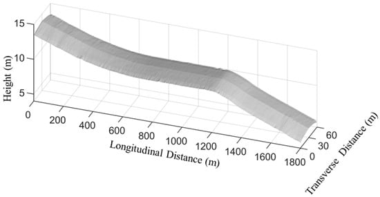
Figure 1.
Elevation profile of Seletar Airport.
2.1.2. Calculation of Water Film Thickness Distribution
The spatiotemporal evolution of runway water film thickness can be depicted using the two-dimensional shallow-water equations [15]. The conservation form of the equations is presented in Equations (1)–(9):
where h is the water film thickness (m), u and v are the horizontal component of water velocity along the x and y directions, respectively (m/s), qr is the rainfall intensity (m/s), g is the gravity constant (m/s2), S0 is the bed slope, Sf is the friction term, z is the pavement elevation (m), nc is the Manning roughness coefficient, and t is time (s). The vectors are defined as: U: conserved variables; F: flux in x-direction; G: flux in y-direction; Q: source term.
The finite volume method and the Harten–Lax–van Leer (HLL) approximate Riemann solver [16,17] are employed to solve the two-dimensional shallow-water equations. For a given pavement elevation and rainfall intensity, the spatiotemporal evolution of water film thickness can be determined. Based on the initial calculation results, the water film thickness sensing data and adjoint-equation method are applied to modify the model results, ultimately obtaining an accurate area distribution of runway water film thickness. The specific algorithm details and calculation processes can be found in our previous research [6,18].
2.1.3. Water Film Thickness Distribution of Seletar Airport
As the sensor placement occurs before practical data collection, this study uses simulated data to design the placement scheme. During simulation, rainfall intensity is set to a constant 3 mm/h, the Manning coefficient to 0.013, the rainfall duration to 120 s, and the output time step to 1 s. This constant intensity was selected because the optimal sensor placement criterion (information entropy) depends primarily on the relative magnitude of water film thickness between locations, which remains stable across rainfall intensities. The value of 3 mm/h corresponds to the 5-year return period and 5 min duration design rainfall standard for Shanghai, China.
Through the use of the above parameters to solve the two-dimensional shallow-water equations and considering the practical placement points, the final calculation results are output at 5 m intervals crosswise and 10 m intervals lengthwise. In this way, the time-varying water film thickness data for 2353 (13 × 181) grid points are obtained, as shown in Figure 2. Note that this distribution at the 120th second represents a quasi-steady state under constant rainfall intensity. When rainfall duration exceeds the time required for runoff equilibrium (approximately 120 s in this configuration), the water film thickness distribution stabilizes with longitudinal uniformity due to balanced drainage intensity across the runway. In the subsequent sections, the water film thickness calculated from this step is considered as the true value.
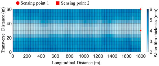
Figure 2.
The true water film thickness distribution at the 120th second.
To simulate the sensor measurement, a random error with a mean of 0 mm and a variance of 0.5 mm is added to the true values calculated above. The error distribution parameters are derived from the field sensor measurement test [13]. The error-adjusted water film thickness values are used as the actual sensor measurements. Figure 3 shows the time variation in the true and measured values for sensing points 1 and 2 from Figure 2. In practice, the measured data will be used to estimate the water film thickness distribution across the entire runway. The goal of optimizing sensor placement is to adjust sensor quantity and location so that the estimated water film thickness value can be as close as possible to the true value.
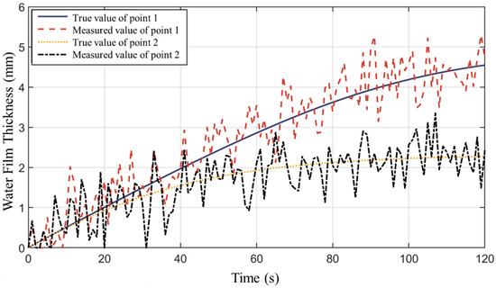
Figure 3.
True value and estimated value at sensing points 1 and 2.
Figure 2 shows that the water film thickness distribution on the airport runway is spatially heterogeneous. The thickness increases from the runway centerline to the shoulders in the transverse direction, while it remains relatively uniform in the longitudinal direction. This transverse heterogeneity arises from the cross-slope design: Runoff originates near the centerline (higher elevation), flowing along the resultant slope direction. Points farther from the centerline experience longer drainage paths, accumulating thicker water films. Longitudinal uniformity occurs because points along the same profile share similar drainage path lengths. This spatial variability causes differences in the signal-to-noise ratio of sensor data at various sensing points (see Figure 3), affecting the accuracy of the estimated water film thickness. To address this, information theory is adopted to study the optimal placement of a single water film thickness sensor and the cooperative placement of multiple sensors.
2.2. Single-Sensor Optimal Placement Method Based on Information Entropy
2.2.1. Information Entropy Calculation Method
Information entropy H(X) measures system uncertainty or information quantity, describing the uncertainty of a random variable through its probability distribution [19,20]. For water film thickness at various points on an airport runway, higher information entropy indicates more information quantity over time. Mutual information T(X, Y) quantifies the information transfer between different points. Higher mutual information indicates more significant spatial variability in water film thickness captured at that point. To determine the optimal placement of a single water film thickness sensor, the sum of the information entropy at the point and the mutual information with other points should be maximized. The objective function is as follows:
where Xi is the time series data obtained by the sensor at sensing point i, n is the total number of grid points, o is the analysis sensing point, H(Xo) is the information entropy of the analysis sensing point, T(Xi, Xo) is the mutual information between the analysis sensing point and other points, and T(X1, X2, …, Xn; Xo) is the total information quantity at the analysis sensing point.
The information entropy H(X) of the sensing point can be calculated using the time series data of the water film thickness, according to Equation (11):
where pi is the probability of the occurrence of the data, and n is the number of data groups.
The equal-interval method is used to determine the occurrence probability of water film thickness data. The range of the time series data X is divided into equal intervals, and the number of samples in each interval divided by the total number of samples gives the probability of occurrence for that interval. This provides the distribution probability over the entire time series. The number of data groups can be calculated using Sturges’ formula [21] as follows:
where m is the total number of sampling points for the time series data.
The mutual information T(X, Y) can be calculated by Equations (13) and (14):
where l and m are the total number of sampling points for the time series data X and Y, respectively.
Through the use of Equations (10)–(14), the total information quantity obtained by a single sensor at various positions of the runway can be calculated. The location with the maximum total information quantity is the optimal placement for a single sensor.
2.2.2. Experimental Validation of Single-Sensor Optimal Placement
To verify the effectiveness of the optimal single-sensor deployment algorithm, a rain and fog experiment was designed. The experiment was conducted at the Intelligent Connected Vehicle South Campus test site of Tongji University. Preparatory steps before the formal experiment were as follows:
- The pavement texture was scanned to obtain parameters such as elevation and slope of the test site.
- The site was equipped with rain and fog spraying devices to simulate real rainfall conditions, which must be pre-adjusted for various parameters.
- Two mobile MD-30 pavement sensors were used in the experiment, referred to as Sensor A and Sensor B. Sensor A was fixed to analyze the impact of different deployment positions on water film accuracy, while Sensor B was mobile and used to obtain the water film thickness reference values (ground truth) at each test point. The instrument layout is shown in Figure 4A.
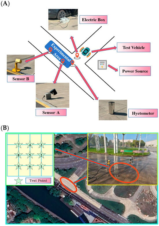 Figure 4. Instrument layout (A) and test point deployment details (B).
 - Nine test points (~)were arranged on site based on their information entropy. These test points show an increasing trend in their information entropy from to . Data at each test point was collected for one minute. To eliminate disturbances caused by sensor relocation, the average value of the data from the last 35 s of each test period was taken as the actual measured water film thickness at that point. Test point deployment details are shown in Figure 4B.
After the preparations, the rain and fog system was activated. Once a stable and distinct water film was formed, the following experimental steps were carried out:
Step 1: According to a given pavement elevation and rainfall intensity, the two-dimensional shallow-water equations were solved, leading to a preliminary spatiotemporal distribution of water film thickness denoted as Data_pre.
Step 2: Sensor A was placed at a test point and begun measuring the water film at that point. The measured data was recorded as (i = 1, 2,…, 9).
Step 3: Sensor B was placed at the other eight points not occupied by Sensor A to measure the water film thickness. The data collected was recorded as (i = 1, 2,…, 9).
Step 4: Based on from Sensor A, Data_pre were corrected and updated, denoted as . Predicted values were compared with the actual values to calculate the average error (i = 1, 2,…, 9).
Step 5: Steps 2–4 were repeated until Sensor A had been placed at all nine points. This yielded the overall prediction error metrics ~ for each sensor placement.
After the experiment, the measured water film thickness values at the nine test points (~) obtained by Sensor A were denoted as Data_fund. The corresponding prediction errors ~ were sorted in ascending order according to Data_fund, and the distribution charts below were created.
In the figures, the horizontal axis (Index) represents the test points sorted in ascending order by their measured water film thickness. The blue line in Figure 5A shows the sorted measured values of Sensor A at test points 1–9. As calculated in the previous section, the total information quantity increases in this order, and the actual water film thickness values also show an increasing trend. This matches the conclusion that greater information entropy corresponds to higher water film thickness.
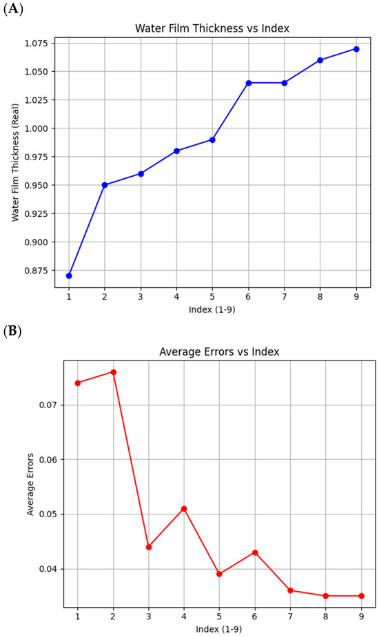
Figure 5.
Measured (actual values) water film thickness at test points (A) and predicted errors of water film thickness at test points (B).
Further analysis of the prediction errors between the predicted and actual water film distributions yields the red line in Figure 5B. It can be observed that when the sensor is placed at points with higher information entropy (or higher water film thickness), the predicted surface distribution becomes more accurate. This demonstrates the reliability of determining optimal sensor placement based on information entropy.
2.3. Multi-Sensor Optimal Placement Method Based on the Correlation Coefficient–Distance Model
For single-sensor water film thickness sensing, the sensor should be placed at the position with the highest total information quantity. However, with multiple sensors, high-information positions may be close together. Simply ranking by total information can cause crowded placement points and local information redundancy.
Therefore, for multi-sensor cooperative sensing of water film thickness, the impact range of sensors must be considered. This study uses the correlation coefficient–distance (C-D) model to determine the impact range [22]. Correlation reflects the relationship between two sets of time series data. A higher correlation coefficient between Location A and Location B indicates that estimating Location A’s water film thickness by Location B’s sensor data is more credible, signifying greater sensor redundancy. Based on this approach, the impact range of sensors can be determined by calculating the correlation coefficients at different distances. The formula for calculating the sensor correlation coefficient is as follows:
where X and Y denote the time series data from different sensing points, d is the distance between the points, A and B are the coordinates of the sensing points, and r is the absolute value of the correlation coefficient between X and Y, with 0 ≤ r ≤ 1.
By plotting the relationship between sensor correlation coefficients and sensor spacing, the impact radius of each sensor can be determined. If the distance between the target point and the sensing point is within this radius, the water film thickness at the target point can be accurately estimated using data from the sensing point. Conversely, if the distance exceeds the impact radius, the estimation accuracy may decrease due to insufficient data correlation. Thus, the principle of multi-sensor optimal placement is to ensure that no other sensors are within the impact radius of each sensor and to maximize the total information gathered from each sensor location.
2.4. Optimization Process for Water Film Thickness Sensor Placement
Based on the results of the total information and the correlation coefficient–distance calculation, the optimal placement scheme for water film thickness sensors can be determined. The specific process is as follows:
Step 1: Obtain airport runway elevation data and simulated rainfall data. Grid the runway area according to sensing requirements and use the two-dimensional shallow-water equation to solve the spatiotemporal evolution of water film thickness at each grid point.
Step 2: Use the results from Step 1 as the true values of the water film thickness. Introduce sensor error distribution data and use these results as the sensor measurements.
Step 3: Calculate the total information at each grid point on the runway using Equations (10)–(14). Calculate the correlation coefficient and distance relationships between grid points using Equations (15) and (16) and determine the sensor’s impact radius.
Step 4: Determine the number of sensors to be deployed based on project budget and actual sensing needs.
Step 5: Develop the sensor placement scheme based on the strategy of placing no other sensors within the impact radius of each sensor and maximizing the total information at each sensor location.
3. Results and Discussion
Seletar Airport was chosen for the case study, and the information distribution of the runway under simulated conditions was obtained. In the simulation, the time series sample length for each point was 120. According to Formula (12), the sample was divided into eight groups. The processed data was used to calculate the total information quantity of each grid point according to Equations (10)–(14). The total information quantity distribution map and the top-6 grid points with the highest total information quantities are shown in Figure 6.
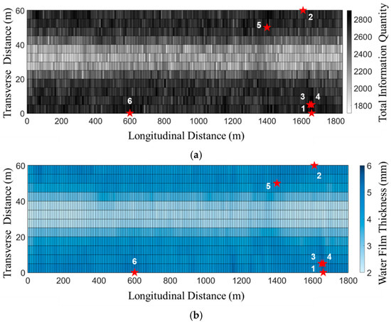
Figure 6.
Total information quantity distribution for Seletar Airport: (a) total information quantity and top-6 optimal placement points; (b) water film thickness and top-6 optimal placement points.
By combining the results from Figure 6a,b, it can be observed that the points with higher total information quantity are mainly located in the areas with thicker water film (as shown in the darker-blue regions in Figure 6b). This occurs because thicker water film yields higher signal-to-noise ratios in sensor data, thus containing more information. Deploying multiple sensors based solely on maximum total information quantity may result in crowded points and information redundancy, as seen with points 1, 3, and 4 in Figure 6.
Through the use of Equations (15) and (16), the correlation coefficients of sensing data at different sensor locations were calculated. For the simulated conditions of Seletar Airport, due to the large number of calculation points, the mutual information for identical sensor spacing was averaged for easier data analysis. The relationship between mutual information and sensor spacing is depicted in Figure 7.
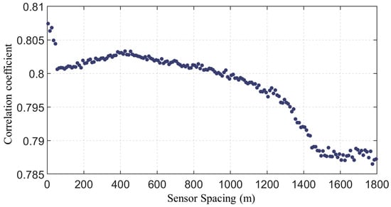
Figure 7.
C-D scatter figure for water film thickness sensor.
The results indicate that within the 1800 m sensing range, the temporal variations in water film thickness at different sensing points are minimal, with all correlation coefficients above 0.785. The correlation coefficients generally decrease as the distance between sensing points increases. The C-D scatter plot reveals that, ignoring the sensor spacing under 50 m, the correlation coefficient peaks when the sensor spacing is around 400 m. At the sensor spacing around 1200 m, the decreasing rate of the correlation coefficient increases, and at around 1500 m, the decrease becomes more sharp. Therefore, in the current analysis scenario, the optimal impact radius of the sensors is set at 400 m, the recommended impact radius at 1200 m, and the extreme impact radius at 1500 m.
Based on the results and the previously proposed optimization process for water film thickness sensor placement, the optimal layout schemes for different impact radii are illustrated in Figure 8. Schemes (a) to (c) represent the optimal layouts for impact radii of 400 m, 1200 m, and 1500 m, respectively. Scheme (d) is a single-sensor layout for budget-limited conditions, while Scheme (e) is an equidistant layout, serving as a control scheme without optimization. The errors between the water film thickness calculated by the measured data obtained from various deployment schemes and the true values are summarized in Table 1.
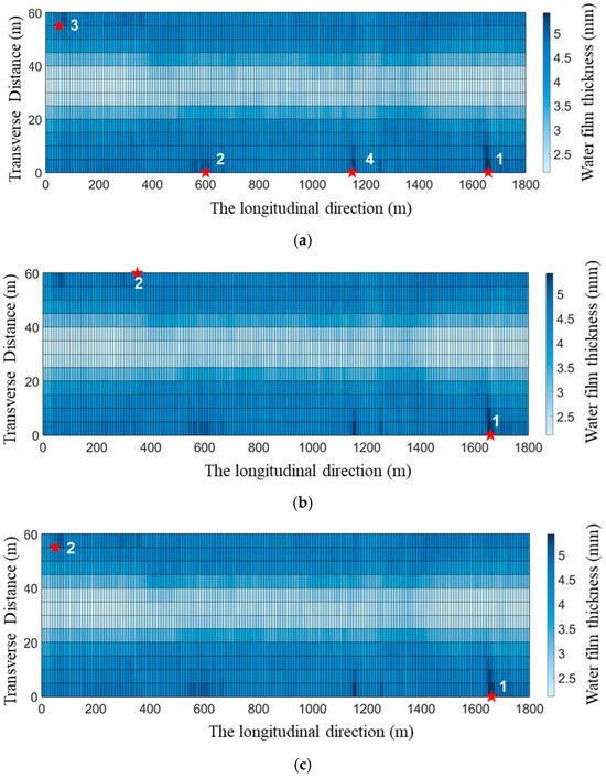
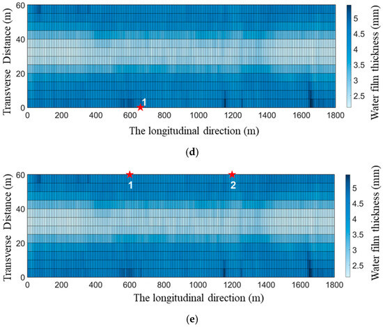
Figure 8.
Deployment schemes for different placement strategies: (a) impact radius = 400 m; (b) impact radius = 1200 m; (c) impact radius = 1500 m; (d) impact radius = 1200 m (single-sensor scheme); (e) scheme without optimization (baseline scheme).

Table 1.
Estimation error for different deployment schemes.
The results indicate that, with an optimal impact radius of 400 m, four water film thickness sensors are needed to ensure complete coverage of the runway. At this radius, the accuracy of the surface water film thickness estimation is the highest, with a relative error of only 4.1%. This represents a 44.6% improvement in accuracy compared to the non-optimized layout Scheme (e). When the impact radius is set to 1200 m or 1500 m, only two sensors are necessary to cover the entire runway. Although this reduces the accuracy slightly, it cuts the number of sensors by 50%, significantly lowering the system cost. Compared to Scheme (e), this approach improves the accuracy of water film thickness estimation by over 23.0%. In Scheme (d), a single sensor can cover the entire runway, but the estimation accuracy is the lowest, with a relative error of up to 10.1%. This could lead to even higher errors in practical applications, diminishing the overall reliability of the sensing system. Overall, the calculations suggest that increasing the number of sensors improves the estimation accuracy of the water film thickness. When budget permits it, increasing the number of sensors can enhance the effectiveness of collaborative sensing.
4. Conclusions
This study proposes an optimization method for water film thickness sensor placement on airport runways to meet the demands of water film thickness monitoring. By integrating information theory with spatial correlation modeling, a novel sensor deployment methodology was developed and validated through numerical simulations and experimental testing. The principal conclusions are summarized as follows:
(1) The information entropy maximization method quantifies the informational value of each grid point, with total information quantity serving as the optimization criterion (Equations (10)–(14)). Theoretical analysis demonstrates that areas with thicker water film (>1.5 mm in this study) exhibit 25–40% higher information entropy compared to thinner regions. Consequently, single sensors should prioritize deployment in deeper water accumulation zones (typically near runway shoulders) to capture high-signal-to-noise-ratio data critical for model correction.
Building upon single-sensor optimization theory, the correlation–distance (C-D) model was introduced to resolve multi-sensor spatial deployment challenges (Equations (15) and (16), Figure 7). The C-D model determines the sensor impact radius, enabling strategic spacing that maintains ≥92% spatial coverage accuracy while minimizing monitoring overlap. This approach reduces sensor deployment requirements by 50% compared to conventional uniform layouts, yielding significant cost savings.
(2) A rain–fog experiment validated the single-sensor deployment methodology. Nine test points were established, with total information quantity calculated for each point using the proposed entropy theory. Sensor measurements combined with the water film distribution algorithm yielded predicted and actual water film thickness values. After correction and analysis, average estimation errors were ranked for each deployment point. The experimental results demonstrated that the ranking based on information entropy aligned with the ranking of prediction errors. This confirms that locations with greater water film thickness yield higher information quantity and superior prediction accuracy. Consequently, single sensors should be installed in areas prone to higher water accumulation.
(3) Through the use of Singapore’s Seletar Airport as a case study, the information quantity distribution and sensor impact radius were scientifically determined. The results confirm that high-information locations correspond to thicker-water-film areas. Under simulated conditions, the optimal sensor impact radius is 400 m, the recommended radius is 1200 m, and the extreme radius is 1500 m. These thresholds enable optimized sensor placement under varying constraints.
Comparative analysis of deployment schemes demonstrates that increased sensor quantity improves estimation accuracy when budget permits it. The proposed method achieves >23.0% higher accuracy compared to non-optimized deployments using identical sensor counts. While single-sensor schemes are cost-effective, their accuracy is significantly compromised by measurement errors (relative error ≤ 10.1%). This optimization method effectively enhances water film thickness estimation accuracy and provides a scientific foundation for designing sensing systems under diverse budget constraints.
Limitations and future work: While effectively addressing sensor placement optimization, this study still has two primary limitations: (i) computational constraints in the water film distribution algorithm limit real-time application on large-scale runways; (ii) longitudinal placement constraints (e.g., mandatory shoulder installations) were not incorporated in the optimization framework. Future research will focus on AI-enhanced high-efficiency algorithms and multi-objective optimization integrating operational constraints.
Author Contributions
The authors confirm contribution to the paper as follows: study conception and design: J.C. and R.Z.; data collection: R.Z. and D.Y.; analysis and interpretation of results: J.C. and D.Y.; draft manuscript preparation: J.C. Supervision, writing-review editing: W.O. and M.Z. All authors have read and agreed to the published version of the manuscript.
Funding
This study was supported by Shanghai Pujiang Programme (23PJD043), Shanghai Urban Digital Transformation Special Fund Project (202401069), Shanghai 2023 Annual “Science and Technology Innovation Action Plan” Social Development Science and Technology Challenge Project (23DZ1202901) and Shanghai Rising-Star Program (24QB2703000).
Institutional Review Board Statement
Not applicable.
Informed Consent Statement
Not applicable.
Data Availability Statement
The original contributions presented in this study are included in the article Further inquiries can be directed to the corresponding author.
Acknowledgments
During the preparation of this work, the authors used ChatGPT4.0 to improve language quality. After using this tool, the authors reviewed and edited the content as needed and take full responsibility for the content of the publication.
Conflicts of Interest
Author Wei Ouyang was employed by the company PowerChina Road & Bridge Group Co., Ltd. The remaining authors declare that the research was conducted in the absence of any commercial or financial relationships that could be construed as a potential conflict of interest.
References
- International Civil Aviation Organization. 2023 Safety Report; ICAO: Montréal, QC, Canada, 2023. [Google Scholar]
- Boyd, D.D. A Review of General Aviation Safety (1984–2017). Aerosp. Med. Hum. Perform. 2017, 88, 657–664. [Google Scholar] [CrossRef]
- Van Es, G.W.H. Running out of Runway: Analysis of 35 Years of Landing Overrun Accidents. NLR TP 2005, 498, 18–19. [Google Scholar]
- Zhao, L.; Zhao, H.; Cai, J. Tire-Pavement Friction Modeling Considering Pavement Texture and Water Film. Int. J. Transp. Sci. Technol. 2023, 14, 99–109. [Google Scholar] [CrossRef]
- Chu, L.; Fwa, T.F. Incorporating Pavement Skid Resistance and Hydroplaning Risk Considerations in Asphalt Mix Design. J. Transp. Eng. 2016, 142, 04016039. [Google Scholar] [CrossRef]
- Cai, J.; Zhao, H.; Qian, X.; Wu, M.; Qian, J. Estimation Method for Area Distribution of Water Film Thickness on Airport Runway Modified by Measured Data in Real Time. J. Traffic Transp. Eng. 2023, 23, 105–114. [Google Scholar]
- Kogbara, R.B.; Masad, E.A.; Kassem, E.; Scarpas, A.T.; Anupam, K. Parameters Influencing Measurement and Modeling of Skid Resistance of Asphalt Pavements. Constr. Build. Mater. 2016, 114, 602–617. [Google Scholar] [CrossRef]
- Civil Aviation Administration of China. China Civil Airport Airfield Maintenance Technical Guide (AC-140-CA-2010-3); CAAC: Beijing, China, 2010. [Google Scholar]
- Najafi, S.; Flintsch, G.W.; McGhee, K.K. Assessment of operational characteristics of continuous friction measuring equipment (CFME). Int. J. Pavement Eng. 2013, 14, 706–714. [Google Scholar] [CrossRef]
- American Association of State Highway and Transportation Officials (AASHTO). Guide for Pavement Friction; AASHTO: Washington, DC, USA, 2020. [Google Scholar]
- Gerthoffert, J.; Grosjean, C.; Cerezo, V.; Do, M.-T. Modelling of Aircraft Braking Coefficient from IMAG Friction Measurements. Airpt. Urban Netw. 2014, 33, 1–11. [Google Scholar]
- Federal Aviation Administration. Runway Condition Assessment Matrix (RCAM); FAA: Washington, DC, USA, 2016. [Google Scholar]
- International Civil Aviation Organization. Global Reporting Format (GRF) for Runway Surface Conditions; ICAO: Montréal, QC, Canada, 2021. [Google Scholar]
- Civil Aviation Administration of China. Notification on the Issuance of Rules for the Assessment and Reporting of Runway Surface Conditions at Transport Airports; CAAC: Beijing, China, 2021. [Google Scholar]
- Sun, L. Research on IRS21 Intelligent Pavement Condition Sensor. Master’s Thesis, Southeast University, Nanjing, China, 2009. [Google Scholar]
- Ewan, L.; Al-Kaisy, A.; Veneziano, D. Remote Sensing of Weather and Road Surface Conditions: Is Technology Mature for Reliable Intelligent Transportation Systems Applications? Transp. Res. Rec. 2013, 2329, 8–16. [Google Scholar] [CrossRef]
- Vyas, V.; Patil, V.J.; Singh, A.P.; Srivastava, A. Application of infrared thermography for debonding detection in asphalt pavements. J. Civ. Struct. Health Monit. 2019, 9, 325–337. [Google Scholar] [CrossRef]
- Bi, Y.; Pei, J.; Guo, F.; Li, R.; Shi, N. Implementation of Polymer Optical Fibre Sensor System for Monitoring Water Membrane Thickness on Pavement Surface. Int. J. Pavement Eng. 2019, 22, 872–881. [Google Scholar] [CrossRef]
- Wosniok, A. POF Sensors for Structural Health Monitoring. In Plastic Optical Fiber Sensors; CRC Press: Boca Raton, FL, USA, 2019; pp. 267–283. [Google Scholar]
- Sahota, J.K.; Gupta, N.; Dhawan, D. Fiber Bragg grating sensors for monitoring of physical parameters: A comprehensive review. Opt. Eng. 2020, 59, 060901. [Google Scholar] [CrossRef]
- Yu, C.; Duan, J. Two-Dimensional Hydrodynamic Model for Surface-Flow Routing. J. Hydraul. Eng. 2014, 140, 04014045. [Google Scholar] [CrossRef]
- Ressel, W.; Wolff, A.; Alber, S.; Rucker, I. Modelling and Simulation of Pavement Drainage. Int. J. Pavement Eng. 2019, 20, 801–810. [Google Scholar] [CrossRef]
- Harten, A. On a Class of High Resolution Total-Variation-Stable Finite-Difference Schemes. SIAM J. Numer. Anal. 1984, 21, 1–23. [Google Scholar] [CrossRef]
- Chen, X.; Zhang, X.; Li, J.; Ren, M.; Zhou, B. A new method for automated monitoring of road pavement aging conditions based on recurrent neural network. IEEE Trans. Intell. Transp. Syst. 2022, 23, 24510–24523. [Google Scholar] [CrossRef]
- Cai, J.; Zhao, H.; Zhu, X.; Cao, J. Wide-Area Dynamic Sensing Method of Water Film Thickness on Asphalt Runway. J. Test. Eval. 2020, 48, 20190172. [Google Scholar] [CrossRef]
- Yang, W.; Tian, B.; Fang, Y.; Wu, D.; Zhou, L.; Cai, J. Evaluation of Highway Hydroplaning Risk Based on 3D Laser Scanning and Water-Film Thickness Estimation. Int. J. Environ. Res. Public Health 2022, 19, 7699. [Google Scholar] [CrossRef]
- Bhaskar, J.; Suribabu, C.R. Estimation of surface run-off for urban area using integrated remote sensing and GIS approach. Jordan J. Civ. Eng. 2014, 8, 70–80. [Google Scholar] [CrossRef]
- Jaynes, E.T. Information Theory and Statistical Mechanics. Phys. Rev. 1957, 106, 620–630. [Google Scholar] [CrossRef]
- Vargas, E. Shallow-Water Sensor Placement; Naval Postgraduate School: Monterey, CA, USA, 2022. [Google Scholar]
- Ma, J.; Wang, Y.; Niu, X.; Jiang, S.; Liu, Z. A comparative study of mutual information-based input variable selection strategies for the displacement prediction of seepage-driven landslides using optimized support vector regression. Stoch. Environ. Res. Risk Assess. 2022, 36, 3109–3129. [Google Scholar] [CrossRef]
- Székely, G.J.; Rizzo, M.L.; Bakirov, N.K. Measuring and Testing Dependence by Correlation of Distances. Ann. Stat. 2007, 35, 2769–2794. [Google Scholar] [CrossRef]
- Wang, S.; Zhang, X.; Wang, J.; Tao, T.; Xin, K.; Yan, H.; Li, S. Optimal sensor placement for the routine monitoring of urban drainage systems: A re-clustering method. J. Environ. Manag. 2023, 335, 117579. [Google Scholar] [CrossRef] [PubMed]
- Barrett, M.L.; Pigman, J.G. Evaluation of Automated Bridge Deck Anti-Icing System; No. KTC-01-26/KH 36-97-1F; 2001. Available online: https://rosap.ntl.bts.gov/view/dot/15875 (accessed on 19 August 2025).
- Chang, N.B.; Guo, D.H. Urban flash flood monitoring, mapping and forecasting via a tailored sensor network system. In Proceedings of the 2006 IEEE International Conference on Networking, Sensing and Control, Ft. Lauderdale, FL, USA, 23–25 April 2006; pp. 757–761. [Google Scholar]
Disclaimer/Publisher’s Note: The statements, opinions and data contained in all publications are solely those of the individual author(s) and contributor(s) and not of MDPI and/or the editor(s). MDPI and/or the editor(s) disclaim responsibility for any injury to people or property resulting from any ideas, methods, instructions or products referred to in the content. |
© 2025 by the authors. Licensee MDPI, Basel, Switzerland. This article is an open access article distributed under the terms and conditions of the Creative Commons Attribution (CC BY) license (https://creativecommons.org/licenses/by/4.0/).