DyP-CNX: A Dynamic Preprocessing-Enhanced Hybrid Model for Network Intrusion Detection

Abstract

With the continuous growth of network threats, intrusion detection systems need to have robustness and adaptability to effectively identify malicious behaviors. However, factors such as noise interference, class imbalance, and complex attack pattern recognition have posed significant challenges to traditional systems. To address these issues, this paper proposes a dynamic preprocessing-enhanced DyP-CNX framework. The framework designs a sliding window dynamic interquartile range (IQR) standardization mechanism to effectively suppress the temporal non-stationarity interference of network traffic. It also combines a random undersampling strategy to mitigate the class imbalance problem. The model architecture adopts a CNN-XGBoost collaborative learning framework, combining a dual-channel convolutional neural network (CNN) and two-stage extreme gradient boosting (XGBoost) to integrate the original statistical features and deep semantic features. On the UNSW-NB15 and CSE-CIC-IDS2018 datasets, the method achieved F1 values of 91.57% and 99.34%, respectively. The experimental results show that the DyP-CNX method has the potential to handle the feature drift and pattern confusion problems in complex network environments, providing a new technical solution for adaptive intrusion detection systems.

1. Introduction

As cyber attacks become increasingly sophisticated and prevalent, protecting sensitive information and ensuring the normal operation of organizations have become significant challenges. Among various forms of cyber threats, intrusion behaviors serve as particularly covert and dangerous attack vectors, embedded within network traffic and posing high risks [1]. As a core line of defense in cybersecurity, the performance of intrusion detection systems (IDS) directly impacts the risk resistance capacity of critical infrastructure in sectors such as finance, healthcare, and energy [2]. However, current IDS technologies encounter three major challenges: Firstly, data-level issues such as noise interference and class imbalance lead to reduced model sensitivity; secondly, at the feature level, there is a bottleneck in extracting the spatiotemporal characteristics of complex attack patterns; and thirdly, the static design of architectures impairs the ability to generalize against zero-day attacks [3].

Under the classic machine learning paradigm, decision trees (DT) offer good interpretability and high training efficiency but are prone to overfitting in noisy data scenarios, significantly reducing performance [4]. Deep learning methods have achieved breakthroughs in detection performance through hierarchical feature abstraction. For example, AE-GRU improves anomaly detection via reconstruction error mechanisms [5], but this model is highly sensitive to initial weight settings, which can cause substantial performance fluctuations. Meanwhile, generative adversarial networks (GANs) generate attack samples via adversarial training [6] but face mode collapse risks during training. Although advanced feature engineering approaches such as CL-FS [7] and BRFE-CBIAT [8] have made progress in feature dimensionality reduction, the disjoint design between feature selection and classifier training results in information loss and weakened model generalization. More fundamentally, existing methods generally employ rigid data processing pipelines lacking adaptive mechanisms to respond to dynamic data distribution changes, leading to systemic failures when facing zero-day attacks and adversarial samples [9]. To address these challenges, this paper proposes a dynamic preprocessing enhanced CNN-XGBoost hybrid model (DyP-CNX), establishing a comprehensive optimization framework from data preprocessing to model architecture, aiming to provide an overall solution for intrusion detection in complex network environments. The main contributions are summarized as follows:

• A fusion of sliding window dynamic IQR estimation and the adaptive random under-sampling (RUS) strategy is implemented to collaboratively optimize distribution parameters and sample weights, effectively improving classification performance on imbalanced network traffic data.
• An incremental feature selection method is introduced, utilizing classical random forest feature importance evaluation combined with a sliding window mechanism to dynamically exclude less important features.
• We propose a CNN-XGBoost cascading architecture that utilizes a dual-channel CNN and a two-stage XGBoost to achieve deep complementarity between local and global features, thereby improving the detection and classification accuracy for complex and covert attack patterns.

The remaining structure of this paper is as follows: Section 2 reviews recent related work in intrusion detection. Section 3 introduces the proposed framework. Section 4 details the experimental datasets, evaluation metrics, and discusses the results. Finally, Section 5 concludes the paper.

2. Related Works

Network intrusion detection has always been a key focus and research area in cybersecurity. With the development of machine learning and deep learning methods, extensive research has been conducted on deep learning-based web anomaly detection. To achieve better detection performance, researchers have focused on designing different feature representation methods and detection models. The main work can be summarized into the following two aspects:

2.1. Data Preprocessing Techniques

In the field of network intrusion detection, data preprocessing techniques have become a hotspot for enhancing model adaptability. Ref. [10] used byte frequency (i.e., the occurrence count of bytes 0–255 in traffic flows) to represent traffic, normalizing these frequencies by dividing them by message length, thereby enabling the detection of low-rate network traffic attacks. Ref. [11] proposed a model that standardizes feature vectors using Z-Score normalization, thereby increasing flexibility in responding to data distribution changes. Ref. [12] introduced an improved DDoS detection method that combines Z-Score with Fast-Entropy statistical metrics and incorporates additional statistical features, significantly improving the accuracy of DDoS detection. However, the Z-Score [13] method can effectively distinguish signal periodicity and detect anomalies, but it introduces latency, which is equal to the size of the chosen time window. Ref. [14] studied the feature optimization of malware data by combining IQR, Document Frequency (TF-IDF), and Recursive Feature Elimination (RFE) and integrated the extracted optimal features into Dueling Deep Q Networks (DDQN) to achieve effective network security threat detection. Ref. [15] proposed a multi-layer network attack/intrusion classification method combining clustering-based under-sampling and random forests, effectively addressing issues of data imbalance and classifier overfitting. However, this approach has only achieved promising experimental results on the KDD 99 benchmark dataset and requires further validation against the continuously evolving network threats.

2.2. Evolution of Model Architecture

Traditional machine learning models such as XGBoost [16], which employ regularized decision tree ensembles, improve detection accuracy; however, their serial growth pattern limits feature interaction capabilities. Although LightGBM [17] accelerates training through histogram-based discretization, it remains sensitive to class imbalance. Deep learning models like SRFCNN-BiLSTM [18], which combine spatiotemporal features to enhance detection performance, are hindered by high computational complexity, restricting their deployment in industrial settings. In Ref. [19], it is pointed out that CNNs can effectively capture spatiotemporal local features in network traffic for intrusion detection, especially in edge computing scenarios. However, these studies are still limited by the single deployment mode of traditional classifiers, resulting in insufficient generalization to complex attack types. Additionally, the XGBoost-based online detection system for Low-rate Denial of Service (LDoS) attacks proposed in [20] demonstrates classification efficiency when processing high-dimensional traffic features, but it still relies directly on raw features and fails to address the robustness challenges caused by high-dimensional sparsity.

3. The Proposed Model

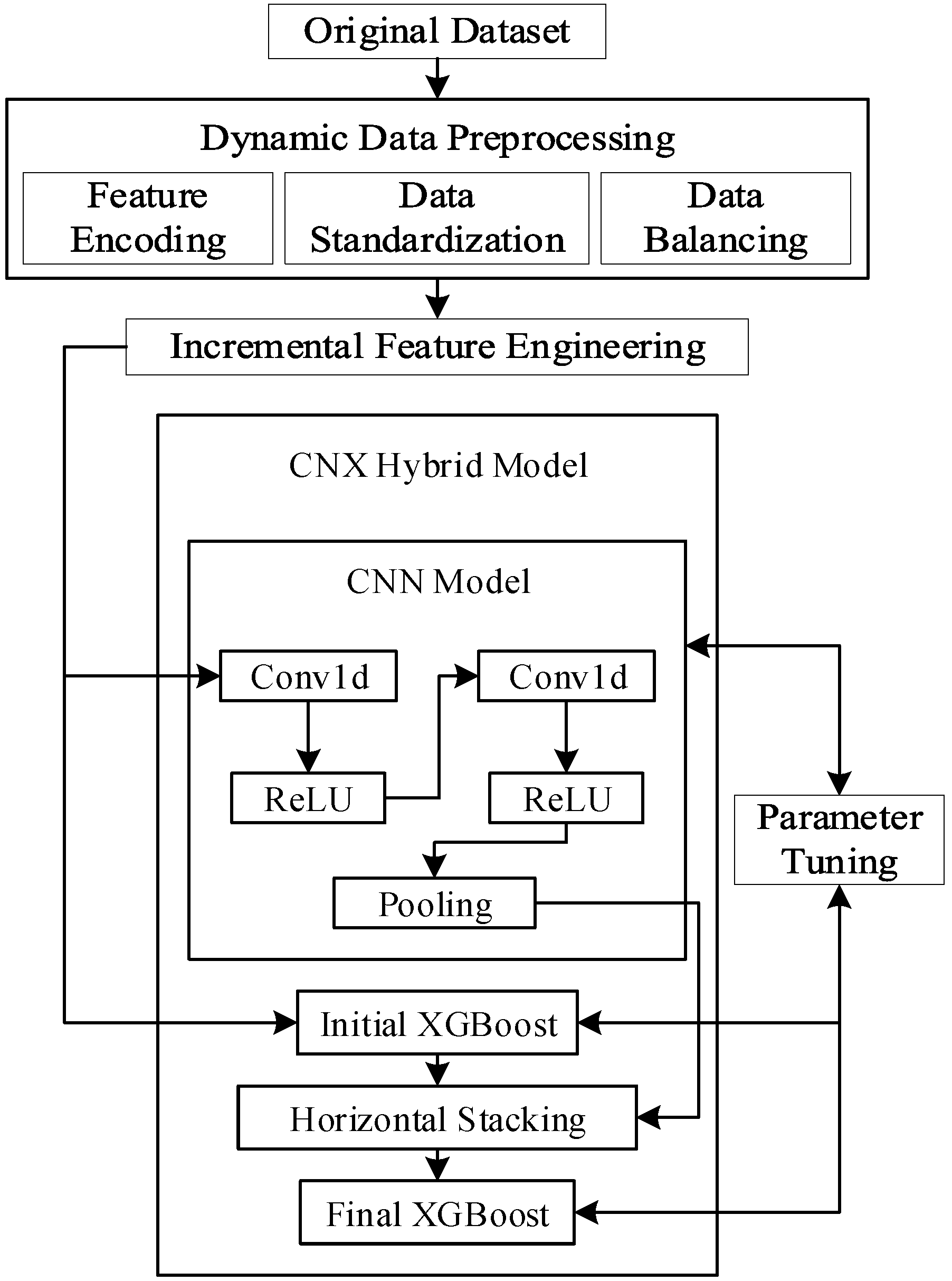
The proposed network intrusion detection framework, DyP-CNX, systematically addresses challenges such as class imbalance, feature redundancy, and complex pattern capture through the design of dynamic data preprocessing and a hybrid model collaborative architecture. The overall framework, shown in Figure 1, comprises four modules: dynamic data preprocessing, incremental feature engineering, the CNX hybrid model, and visualization and evaluation analysis.

3.1. Dynamic Data Preprocessing

The goal of dynamic preprocessing is to remove invalid samples and use ordinal encoding for dimensionality reduction. It applies sliding window-based dynamic IQR to suppress temporal interference and employs random undersampling to balance class proportions, thereby enhancing the detection capability for minority classes. It primarily includes three components: feature encoding, data normalization, and data balancing.

3.1.1. Feature Encoding

This paper employs ordinal categorical encoding [21] to encode non-numeric categorical features in network traffic, such as protocol type (proto), service type (service), and connection status (state). For each categorical feature, an explicit ordinal relationship is constructed based on its semantic meaning, and a numerical mapping is used to preserve the ordinal relations between categories. Compared to one-hot encoding, this method maintains the feature’s entropy while reducing the dimensionality from N (number of categories) to 1, thereby significantly decreasing the computational complexity of subsequent CNN convolution kernels (from O(N) to O(1)).

3.1.2. Data Standardization

Data normalization is a key step to improve model performance. Based on the traditional Robust Scaling method, this paper proposes a sliding window-based dynamic IQR normalization technique, effectively addressing the temporal non-stationarity of network traffic data. The formula for calculating the dynamic IQR is

$$\left\{\begin{array}{c}{\mathrm{IQR}}^{\left(t\right)}=Q_3^{\left(t\right)}-Q_1^{\left(t\right)}\hfill \\ Q_k^{\left(t\right)}=\mathrm{Quantile}\left(W^{\left(t\right)},k/4\right),k\in \{1,3\}\hfill \\ W^{\left(t\right)}=\{x_{t-T+1},x_{t-T+2},\dots ,x_t\}\hfill \end{array}\right.$$

(1)

Among these, T is the size of the sliding window, $W^{\left(t\right)}$ represents the data within the window at time t, and $Q_k^{\left(t\right)}$ is the k-th quartile of the data within the window. The implementation steps are as follows:

Window Initialization: Load the first T samples and compute the initial first quartile $Q_1^{\left(0\right)}$ and third quartile $Q_3^{\left(0\right)}$.

Incremental Update: With each new sample $x_{t+1}$, remove the oldest sample $x_{t-T+1}$ from the window. Based on the updated $W^{(t+1)}$, recompute the IQR.

$$W^{(t+1)}=\left\{\begin{array}{cc}{W}^{\left(t\right)}\cup \left\{x_{t+1}\right\},\hfill & \mathrm{if}|W^{\left(t\right)}|<T\hfill \\ (W^{\left(t\right)}\setminus \left\{x_{t-T+1}\right\})\cup \left\{x_{t+1}\right\},\hfill & \mathrm{if}|W^{\left(t\right)}|\ge T\hfill \end{array}\right.$$

(2)

Dynamic Scaling: $Q_2^{\left(t\right)}$ is the median of the data within the window $W^{\left(t\right)}$.

$$x_{t+1}^{\mathrm{scaled}}={\displaystyle \frac{x_{t+1}-Q_2^{\left(t\right)}}{{\mathrm{IQR}}^{\left(t\right)}}}$$

(3)

This method ensures that the statistical measures reflect only the recent data distribution by limiting the number of samples in the window, thereby preventing long-term interference from historical anomalous data.

3.1.3. Data Balancing

When addressing the issue of class imbalance in training datasets, oversampling and under-sampling techniques play a crucial role. Since real-world data often exhibit uneven class distributions, this can cause the model to favor the majority class during training, thereby reducing its ability to recognize minority class samples. To effectively solve this problem, this paper employs a random under-sampling method. By randomly selecting samples from the majority class, the number of majority class samples is reduced, bringing the sizes of the majority and minority classes closer to balance. The goal is to prevent the model from overfitting to the majority class and to enhance its generalization ability on the test set. Specifically, the mathematical expression of the random under-sampling method is as follows:

$$\left\{\begin{array}{c}C(N_A,N_{\mathrm{target}})={\displaystyle \frac{N_A!}{N_{\mathrm{target}}!(N_A-N_{\mathrm{target}})!}}\hfill \\ D_{\mathrm{new}}=\{x_i\mid x_i\in A, i=1, 2, \dots , N_{\mathrm{target}}\}\cup \{y_j\mid y_j\in B, j=1, 2, \dots , N_B\}\hfill \end{array}\right.$$

(4)

Among these, $N_A$ is the number of samples in the majority class, $N_B$ is the number of samples in the minority class, and $N_{\mathrm{target}}$ is the target number of samples, which is set to $N_B$. $C(N_A,N_{\mathrm{target}})$ denotes the number of combinations for selecting $N_{target}$ samples from $N_A$ samples. $x_i$ represents a sample from class A, $y_j$ represents a sample from class B, and $D_{\mathrm{new}}$ is the new balanced dataset.

By using this approach to obtain a balanced dataset, the model can treat samples from different classes more fairly during training, which can improve the model’s performance on imbalanced data to a certain extent. Additionally, compared to oversampling methods, random under-sampling does not increase the number of samples in the dataset, thereby reducing computational resource consumption and the potential risk of overfitting.

3.2. Incremental Feature Engineering

Feature selection holds an important position in machine learning and data mining, as it can enhance model performance, reduce overfitting, improve interpretability, and accelerate training. This study is based on the classic random forest feature importance evaluation [22], introducing a sliding window mechanism where feature importance is updated after every K samples. The calculation formula is as follows:

$$\left\{\begin{array}{c}{\mathrm{Importance}}^{\left(m\right)}\left(f\right)={\displaystyle \frac{1}{T}}\sum _{i=1}^T\left({\mathrm{MSE}}_{\mathrm{before}}^{(i,m)}-{\mathrm{MSE}}_{\mathrm{after}}^{(i,m)}\right)\hfill \\ m={\displaystyle \frac{\mathrm{Total}\mathrm{number}\mathrm{of}\mathrm{samples}}{K}}\hfill \end{array}\right.$$

(5)

Among these, $T=100$ represents the number of decision trees, m indicates the k-th window, and ${\mathrm{MSE}}^{(i,t)}$ is the mean squared error change of the i-th tree in the t-th window. A Pearson correlation coefficient threshold of $\theta =0.7$ is used, which references Cohen’s d effect size criterion (where ≥0.8 indicates a strong correlation). This setting helps maximize the removal of redundant features, thereby enhancing computational efficiency while preserving a substantial amount of the original information. When the correlation between features $(f_i,f_j)$ satisfies $\rho (f_i,f_j)>\theta$, the less important feature among the pair is removed.

3.3. CNX Hybrid Model

The CNX hybrid model integrates CNN features with XGBoost predicted probabilities. This model consists of three main components: a CNN model, an initial XGBoost classifier, and a final XGBoost classifier. The structure of the initial and final XGBoost classifiers is identical, except for the $n\_estimators$ parameter; all other parameters are the same. The training and prediction process is as follows:

• The raw data first undergo feature extraction through CNN, leveraging CNN’s strong capability in extracting valuable features.
• The raw data are then used by the initial XGBoost to obtain predicted probabilities, enabling it to preliminarily learn the data’s patterns and rules from the original features.
• In the feature fusion design, we adopt a horizontal stacking strategy based on the complementary advantages of CNN, which excels at extracting local spatial features (such as temporal patterns of attack traffic), and XGBoost, which is adept at capturing global statistical characteristics. Subsequently, the outputs of CNN $O_{\mathrm{cnn}}$ and the initial XGBoost $O_{\mathrm{xgb}}$ are combined using a horizontal stacking method to produce a new feature set. This enriched feature representation provides a stronger basis for subsequent classification, allowing the model to leverage the strengths of different models, thereby enhancing overall classification accuracy and generalization ability. The horizontal stacking method is as follows:

  $$\mathrm{CombinedFeatures}=\mathrm{np}.\mathrm{hstack}\left([O_{\mathrm{cnn}},O_{\mathrm{xgb}}]\right)$$

  (6)
• Using the fused features as input, they are fed into the final XGBoost classifier, which further optimizes the model’s performance to better adapt to complex classification tasks and produce the final prediction results, denoted as Prediction, as shown below:

  $$\mathrm{Prediction}=\mathrm{XGBoost}\_\mathrm{final}(\mathrm{CombinedFeatures})$$

  (7)

The model employs a two-stage XGBoost approach, consisting of an initial and a final classifier. This design enables the model to learn in different feature spaces, providing an opportunity to capture more comprehensive data representations. The initial XGBoost directly learns from the original features, while the final XGBoost learns from the high-level features output by the CNN and the predictions of the initial model. This multi-layered learning strategy helps enhance the model’s robustness and overall performance.

3.3.1. CNN Component

The CNN component primarily consists of two convolutional layers and one adaptive average pooling layer. The specific details are as follows:

• Convolutional Layer: The first convolutional layer has an input channel number of in_channels, an output channel number set to 16, a kernel size of 2, and padding of 1. The convolution operation is represented as

  $$Y_1=X\times W_1+b_1$$

  (8)
  Among these, X is the input feature map, $W_1$ is the convolution kernel, $b_1$ is the bias term, × denotes the convolution operation, and $Y_1$ is the output feature map.
  To enable the CNN to better extract features, the shape of the sample data in the dataset was adjusted. Assuming each sample’s feature data make up a one-dimensional structure consisting of K feature combinations, this structure is reshaped into a two-dimensional structure with $N\times M$ feature combinations, making the input channel number in_channels = N, where $K=N\times M$. This method can be viewed as a tensor or matrix decomposition problem. By selecting appropriate (p) and (q), it essentially involves splitting the original spatial dimensions into two parts. This approach is similar to tensor decompositions such as Tucker decomposition, which decompose high-dimensional data into low-dimensional components while preserving the main structure of the data. In this context, the paper converts an arbitrary length 1D feature vector (K) into a 2D structure ($N\times M$) to meet the input requirements of a standard 2D CNN architecture (in_channels = N). The calculation of N and M is as follows:

  $$\left\{\begin{array}{c}F=(a_i,b_i)\mid a_i=i;b_i={\displaystyle \frac{K}{i}};i=1, 2, \dots , \lfloor \sqrt{K}\rfloor ;Kmodi=0\hfill \\ (N,M)=(a_m,b_m);m=\left|F\right|\hfill \end{array}\right.$$

  (9)
  Among these, F is the set of factor pairs, $(a_i,b_i)$ represents the i-th factor pair, and m is the number of such pairs.
  By analyzing sample shapes and choosing suitable factors to configure in_channels, the model can better accommodate different inputs, allowing the CNN to extract features more effectively and, ultimately, improving its performance and generalization capability.
  The input channel number for the second layer is 16, and the output channel number is out_channels (which is an external parameter, as described in the hyperparameter optimization chapter). The convolution kernel size is 2, with padding of 1. Its output is represented as

  $$Y_2=Y_1\times W_2+b_2$$

  (10)
  Among these, $W_2$ is the convolution kernel of the second layer, $b_2$ is the bias term of the second layer, × denotes the convolution operation, and $Y_2$ is the output feature map.
• Pooling Layer: The pooling layer reduces the length of the feature map output by the convolutional layer to 1, which helps in extracting global features and decreasing the feature dimension. The output of this layer can be expressed as

  $$Y_{\mathrm{pool}}=\mathrm{AvgPool}\left(Y_2\right)$$

  (11)
  Among these, $Y_{\mathrm{pool}}$ is the output feature of the pooling layer. Average pooling reduces the dimensionality of the feature map while retaining certain global information, enabling the model to better capture the overall features of the data.
• Activation Function: The activation function selected is the ReLU (Rectified Linear Unit), which is widely used in deep learning. In PyTorch, it is implemented as torch.relu, and its formula is

  $$\mathrm{ReLU}\left(x\right)=max(0,x)$$

  (12)
  Among these, x is the input to the activation function. This activation function outputs the input directly when it is positive and outputs zero when the input is negative. It effectively alleviates the vanishing gradient problem, allowing the model to update parameters more stably during training, thereby improving the training performance and generalization ability of the model.
• Loss Function: The CNN model extracts features from the input data. The training of the CNN uses the crossentropy loss function and the Adam optimizer, and the loss function is expressed as

  $${\mathcal{L}}_{\mathrm{CNN}}=-\sum _{i=1}^N\sum _{j=1}^C{y}_{ij}log\left(p_{ij}\right)$$

  (13)
  Among these, N is the number of samples, C is the number of classes, $y_{\mathrm{ij}}$ is the true label, and $p_{\mathrm{ij}}$ is the predicted probability.

3.3.2. XGBoost Hyperparameters

During the training process, the CNN model extracts features from the data and reshapes them to fit the input format of the XGBoost classifier. The XGBoost classifier is then trained using the reshaped training data and corresponding labels. The key hyperparameters of the XGBoost model are set as follows:

• n_estimators: specifies the number of trees (passed as an external parameter, see hyperparameter optimization chapter).
• learning_rate: controls the contribution of each tree, typically denoted as $\eta$ (passed as an external parameter, see hyperparameter optimization chapter).
• use_label_encoder = False: to avoid using the deprecated label encoder.
• eval_metri c = ‘logloss’: uses log loss as the evaluation metric for binary classification.
• objective = ‘binary:logistic’: specifies the binary logistic regression objective.

The prediction process of XGBoost can be represented as a weighted sum of the predictions of all decision trees:

$$\widehat{y}=\sum _{t=1}^{\mathrm{n}\_\mathrm{estimators}}{f}_t\left(x\right)$$

(14)

Among these, $\widehat{y}$ is the final predicted result, and $f_t\left(x\right)$ is the prediction result of the t-th tree.

The formula for the Log Loss function used by XGBoost is

$$\mathcal{L}=-{\displaystyle \frac{1}{N}}\sum _{i=1}^N\left[y_{i}log\left({\widehat{y}}_i\right)+(1-y_i)log(1-{\widehat{y}}_i)\right]$$

(15)

Among these, N is the number of samples, $y_i$ is the true label, and ${\widehat{y}}_i$ is the model’s predicted probability of the positive class.

XGBoost’s optimization objective is to minimize the following regularized objective function Obj:

$$\mathrm{Obj}=\sum _{i=1}^{n}l(y_i,{\widehat{y}}_i)+\sum _{k=1}^K\Omega \left(f_k\right)$$

(16)

Among these, i is the sample index, l is the loss function, $\Omega$ is the regularization term, and $f_k$ represents the k-th decision tree.

XGBoost incorporates built-in regularization to prevent overfitting and enhance the model’s generalization ability. Its powerful classification performance enables it to achieve excellent results in complex classification tasks.

3.4. Visualization and Evaluation Analysis

Existing studies generally evaluate detection performance using a single metric such as accuracy, which does not fully reflect the true performance of models in scenarios with class imbalance. To address this, this paper constructs a multidimensional evaluation system, employing confusion matrices, receiver operating characteristic (ROC) curves, and quantitative metrics (such as accuracy, F1, etc.) for a more comprehensive assessment of the model’s performance. Additionally, this study introduces t-distributed stochastic neighbor embedding (t-SNE) [23] visualization, which maps high-dimensional data into a low-dimensional space. By comparing and analyzing the changes in data distribution, it provides an intuitive reflection of the effectiveness of the model’s feature learning. t-SNE defines the neighborhood relationships between sample points in high-dimensional space using Gaussian distribution-based conditional probabilities, as shown below:

$$P_{j|i}={\displaystyle \frac{exp\left(-\frac{\parallel x_i-x_j{\parallel }^2}{2{\sigma }_i^2}\right)}{{\displaystyle \sum _{k\ne i}}exp\left(-\frac{\parallel x_i-x_k{\parallel }^2}{2{\sigma }_i^2}\right)}}$$

(17)

Among these, $x_i$ is the baseline data point, $x_j$ is a specific data point, $x_k$ represents all other sample points except $x_i$, and ${\sigma }_i$ is the standard deviation calculated based on the local density around $x_i$.

In the low-dimensional space, t-distribution with fewer degrees of freedom is used to alleviate the “crowding problem.” The low-dimensional distribution is optimized by minimizing the Kullback–Leibler (KL) divergence, as shown below:

$$\mathrm{KL}(P\parallel Q)=\sum _i{P}_{i}log\left({\displaystyle \frac{P_i}{Q_i}}\right)$$

(18)

Among these, P is the true distribution, Q is the model distribution, $P_i$ is the probability of event i occurring in the true distribution, and $Q_i$ is the probability of event i occurring in the model distribution. $KL$ divergence measures the asymmetric difference between the two probability distributions.

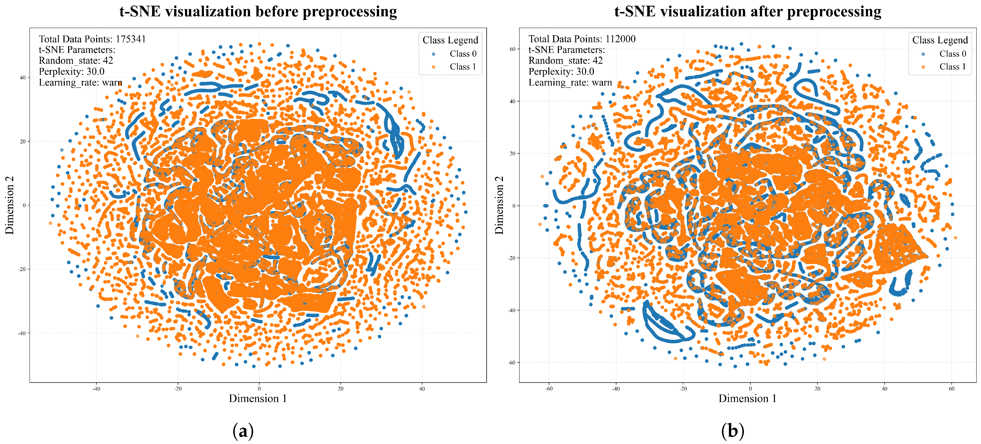
t-SNE visualization effectively reflects the similarity of high-dimensional data and reveals the intrinsic structure of the data. Similar samples form tight clusters, and class boundaries are clear, indicating good separability of features. Conversely, regions with mixed colors highlight potential classification confusions. This analysis validates the model’s adaptability to imbalanced data and provides valuable visual insights for feature optimization and decision boundary adjustments.

4. Experiments and Results

We conducted four experiments to evaluate the performance of the proposed method on three publicly available standard datasets and our experimental environment is the Win10 operating system with i7 CPU processing and 128 GB RAM.

4.1. Datasets

The proposed model was validated on the public datasets UNSW-NB15 and CSE-CIC-IDS 2018, which have been used in numerous papers for network attack detection [7,9,16,17,18].

UNSW-NB15 [24]: it was collected by the Australian Cyber Security Centre in a realworld environment using the IXIA PerfectStorm tool for simulated data capture. It covers nine types of attacks and normal traffic and consists of two .csv files. We use UNSW-NB15_training-set.csv and UNSW-NB15_testing-set.csv as the training set and testing set, respectively. The distribution of specific experimental data samples is shown in

Table 1. Distribution of UNSW-NB15 dataset.

File	Normal	Abnormal	Total
UNSW-NB15_training-set.csv	56,000	119,341	175,341
UNSW-NB15_testing-set.csv	37,000	45,332	82,332

.

CSE-CIC-IDS 2018 [25]: The CSE-CIC-IDS 2018 dataset was jointly created by the Canadian Cyber Security Establishment (CSE) and the Canadian Institute for Cybersecurity (CIC). It includes seven types of complex attacks, such as DDoS, Botnet, and SQL Injection, as well as normal traffic. The dataset contains over 16.2 million samples and spans 10 days of heterogeneous network traffic. More than 80 features, including packet length distribution and session duration, were extracted using CICFlowMeter. In the experiments, 80% of the data is randomly selected as the training set, while the remaining 20% is used as the testing set.

4.2. Evaluation Metrics

The paper selects Accuracy, Precision and F1 as the evaluation metrics for model performance [26]. TP is the number of true positives. TN is the number of true negatives. FP is the number of false positives. FN is the number of false negatives. The formulas are as follows:

$$\mathrm{Accuracy}={\displaystyle \frac{\mathrm{TP}+\mathrm{TN}}{\mathrm{TP}+\mathrm{FP}+\mathrm{TN}+\mathrm{FN}}}$$

(19)

$$\mathrm{Precision}={\displaystyle \frac{\mathrm{TP}}{\mathrm{TP}+\mathrm{FP}}}$$

(20)

$$F_1={\displaystyle \frac{2\times \mathrm{TP}}{2\times \mathrm{TP}+\mathrm{FP}+\mathrm{FN}}}$$

(21)

4.3. Model Parameters and Tuning

Selecting optimal hyperparameters is crucial to model performance, as different combinations can significantly affect accuracy and generalization, making it a key step in enhancing model performance. This paper adopts the grid search method, which involves combining predefined hyperparameter value ranges and training and evaluating models for each combination. The implementation steps of the grid search are as follows:

• Define the hyperparameter value ranges: Based on experience and understanding of the data, determine the possible value ranges for each hyperparameter.
• Generate hyperparameter combinations: Combine all the value ranges to create a grid of all possible hyperparameter sets.
• Model training and evaluation: For each hyperparameter combination, train a model separately.
• Use specific evaluation metrics: such as accuracy, precision and F1. In this study, F1 is chosen for model evaluation.
• Select the best hyperparameter combination: Based on the evaluation results, select the combination yielding the best performance.

Based on the grid search, the final parameters for the CNN and XGBoost models are as shown in

Table 2. Experiment parameters of CNN.

Out_Channels	Learning_Rate	$\mathit{\eta }$	$\mathit{\lambda }$	Batch Size	EPOCH
32	0.001	0.1	0.001	32	100

and

Table 3. Experiment parameters of XGBoost.

Start-N_Estimators	Learning	End-N_Estimators
100	0.01	100

.

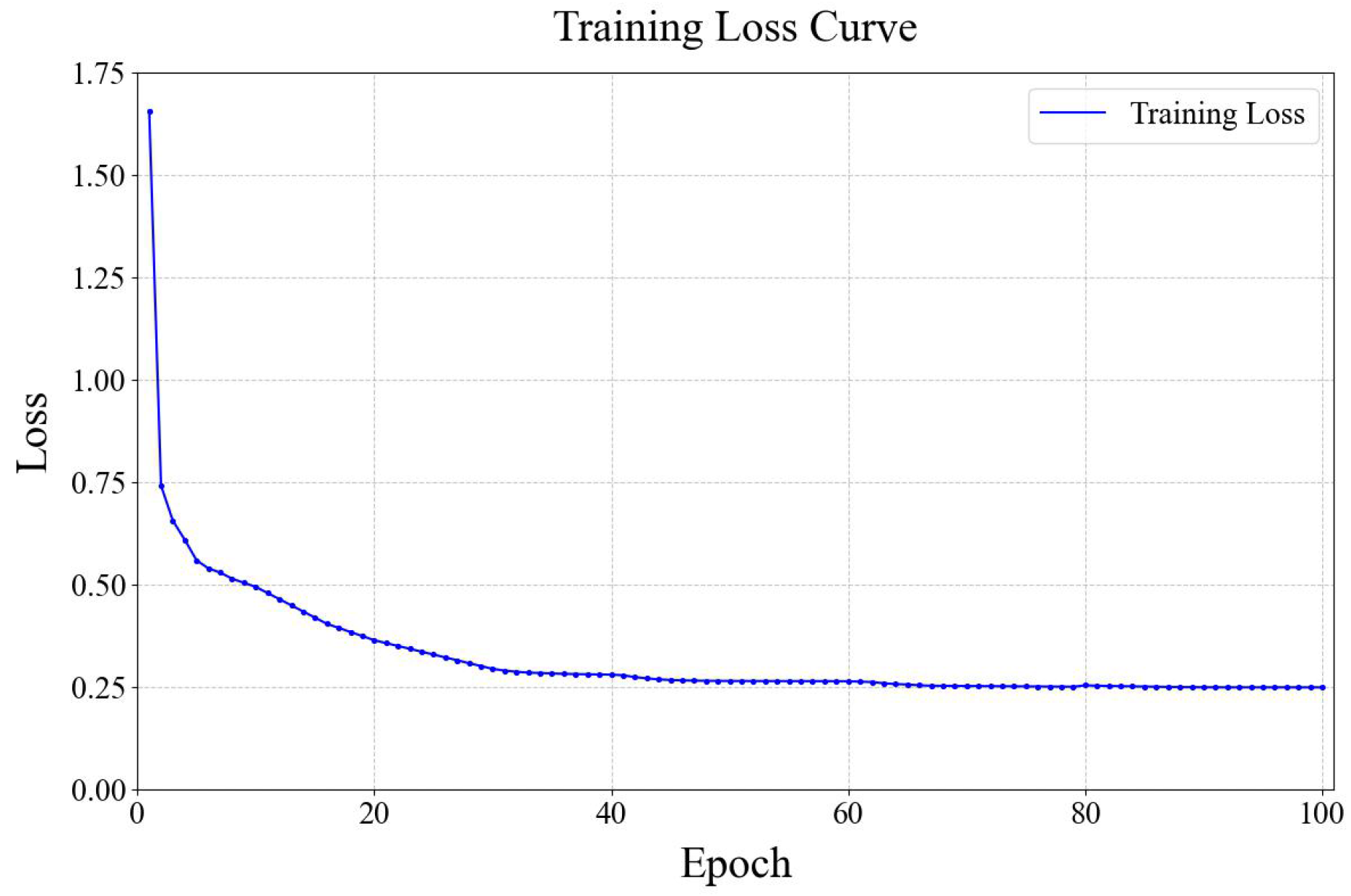
In the experiment, start-n_estimators indicates the initial number of XGBoost trees, while end-n_estimators refers to the final number of trees. The CNN model was trained for 100 epochs, with the training process monitored. The change in training loss is shown in the following Figure 2. From Figure 2, it can be observed that as the training epochs increase, the CNN model’s training loss exhibits a certain trend. Between epochs 80 and 100, the loss decreases slowly, indicating that the chosen parameter is appropriate.

4.4. Experimental Results and Analysis

To comprehensively evaluate the DyP-CNX intrusion detection method, this paper conducts experiments on both the UNSW-NB15 and CSE-CIC-IDS 2018 datasets.

4.4.1. Data Standardization and Feature Engineering

In the data processing stage, data standardization and feature engineering have a significant impact on the detection performance of the model. To enhance model performance, this paper conducts experimental studies on the parameter T in Equation (1) and the parameter K in Equation (5) to determine their optimal values.

To validate the impact of the sliding window size T on model performance, we conducted an analysis using the UNSW-NB15 dataset. In our experiments, we tested three different window sizes: T = 2500, T = 5000, and T = 10,000. We used a random forest (RF) classifier to evaluate how different T values affect the classification performance of samples. The experimental results are shown in the table below.

Based on the experimental results in

Table 4. Data standardization of UNSW-NB15 dataset.

T	Accuracy (%)
2500	89.59
5000	91.04
10,000	90.98

, the choice of window size T = 5000 for the UNSW-NB15 dataset was made after careful consideration because it strikes the best balance between accuracy and computational efficiency. A smaller window (e.g., T = 2500) is more sensitive to local changes but performs slightly worse under noise, causing a drop in accuracy. A larger window (e.g., T = 10,000) can capture more global information but risks overlooking fine details, which also leads to a slight accuracy decrease. T = 5000 effectively combines the advantages of both, raising the model’s accuracy to 91.04%. Therefore, selecting T = 5000 not only improves detection performance but also demonstrates the robustness and adaptability of dynamic IQR normalization.

It is worth noting that the two datasets used in this study differ significantly in sample size (180,000 vs. 9 million), which directly influences the choice of window size. For the smaller UNSW-NB15 dataset, a window size of T = 5000 is more suitable, ensuring faster training and response times while maintaining good performance. For the larger dataset, we chose a window size of T = 50,000, which can more fully utilize the rich temporal information without excessive computational cost.

These choices consider factors such as the dataset scale, temporal variation scale of features, and computational resources, aiming to find the optimal balance between model performance and efficiency for each dataset. The experimental results and analyses provide empirical support for our parameter choices, demonstrating the robustness and effectiveness of the proposed dynamic IQR normalization technique across different window sizes and dataset scales. Additionally, it showcases the adaptability and flexibility of our method when faced with datasets of varying characteristics.

The Spearman correlation coefficient is a nonparametric statistical measure used to assess the strength and direction of the rank relationship between two variables. In this analysis, it is used to compare the consistency of feature importance rankings calculated from adjacent data windows (such as the ith window and the i+1th window).

As shown by the research results in

Table 5. K value selection for UNSW-NB15 dataset.

K	Spearman Correlation Coefficient *	F1 (%)
5000	0.3112	90.77
10,000	0.3469	90.65
15,000	0.3011	90.44
20,000	0.3246	90.43
30,000	0.2328	89.48

* Spearman correlation coefficient is used to measure the strength and direction of a monotonic relationship. A larger absolute value indicates a stronger correlation.

and

Table 6. K value selection for CSE-CIC-IDS 2018 dataset.

K	Spearman Coefficient *	F1 (%)
50,000	0.2583	94.71
100,000	0.2731	94.73
150,000	0.3231	94.72
200,000	0.3323	94.71
300,000	0.2329	94.72

* Spearman correlation coefficient is used to measure the strength and direction of a monotonic relationship. A larger absolute value indicates a stronger correlation.

, our chosen K values (UNSW-NB15: K = 10,000; CSE-CIC-IDS2018: K = 200,000) not only demonstrate excellent performance in terms of model performance (F1-Score), but more importantly, they ensure the high reliability and strong robustness of the feature selection process across the time dimension. This lays a solid foundation for the long-term stable deployment of the model in real-world network environments.

4.4.2. Effects of Data Preprocessing

Figure 3 shows the t-SNE visualization results of the UNSW-NB15 dataset for UNSW-NB15_training-set.csv before and after data preprocessing, respectively. After preprocessing, attack traffic (orange) and normal traffic (blue) exhibit a clear separation in the low-dimensional space. These improvements effectively demonstrate the impact of data preprocessing.

4.4.3. Results on Different Datasets

Initially, we analyzed the UNSW-NB15 dataset and found that some features exhibit a wide range of values. To reduce sensitivity to outliers, this paper employs a dynamic IQR normalization method during feature processing and uses a random forest classifier to preliminarily validate different normalization methods. The results are shown in

Table 7. Comparative analysis of different normalization methods.

Method	F1 (%)	Time_Stability *
DynamicIQR	86.94	0.00302
OnlineZScore	86.85	0.00326
AdaptiveStandard	86.91	0.00337
RunningBatch	86.87	0.00311

* Time_Stability represents standard deviation of accuracy in time series cross-validation.

.

As shown in Table 7, the dynamic IQR method achieved the highest F1 of 86.94% and the lowest Time_Stability of 0.00302, demonstrating its robustness to outliers. This method uses a sliding-window mechanism to update local data distribution characteristics in real time, effectively suppressing the influence of extreme values while maintaining stable computational efficiency.

Moreover, to comprehensively showcase the model’s effectiveness, we conduct an experiment based on the UNSW-NB15 dataset, comparing several mainstream models, including CNN and XGBoost, as well as cuttingedge specialized methods during the past three years of research: AE-GRU [5], CL-FS [7], XGBoost-GRU [16], LightGBM [17], SRF-CNN-BiLSTM [18], and DCNN-LSTM [27]. All methods use the complete dataset and directly cite the best results from the original literature to ensure fair comparison. The experimental results for each method are shown in

Table 8. Comparison on the UNSW-NB15 dataset.

Method	Accuracy (%)	F1 (%)
AE-GRU [5]	88.39	89.00
CL-FS [7]	88.52	88.18
XGBoost-GRU [16]	88.42	87.37
LightGBM [17]	89.54	90.61
SRFCNN-BiLSTM [18]	89.24	90.36
DCNN-LSTM [27]	91.49	81.67
DyP-CNX (Our Method)	92.57	91.57

.

As shown in Table 8, the proposed DyP-CNX method achieves an accuracy of 92.57% and an F1 of 91.57%, surpassing all other comparison methods. This indicates that the model has superior detection capabilities when it comes to identifying anomaly attacks.

Table 9. Computational metrics on the UNSW-NB15 dataset.

Training (s)	Total Inference (s)	Per-Sample Inference (s)
901.07	0.2213	0.000003

presents the computational metrics for the UNSW-NB15 dataset. The training process took approximately 901.07 s, showcasing the efficiency of the DyP-CNX framework in handling complex datasets. Furthermore, the total inference time for the test set was 0.2213 s, translating to an impressive per-sample inference time of 0.000003 s. These metrics indicate that the model is not only robust and accurate but also highly efficient, making it suitable for real-time intrusion detection scenarios where prompt responses are critical. This efficient performance is particularly beneficial in dynamic network environments, where rapid processing and analysis of data streams are essential for maintaining robust security postures.

To further validate the effectiveness of the models, we conducted another experiment based on the CSE-CIC-IDS 2018 dataset, selecting, namely, AI-AWS-RF [9], CLHF [28], and PCA-DNN [29], which have shown outstanding performance on this dataset, for comparison with our proposed method. All methods used the complete dataset and directly adopted the best results from the original literature to ensure fairness in comparison. The experimental results of each method are shown in

Table 10. Comparison on the CSE-CIC-IDS 2018 dataset.

Method	Accuracy (%)	F1 (%)
AI-AWS-RF [9]	97.00	97.00
CLHF [28]	98.53	99.00
PCA-DNN [29]	97.93	98.68
DyP-CNX (Our Method)	98.82	99.34

. As shown in Table 10, the overall performance metrics of the proposed DyP-CNX in this paper are as follows: accuracy of 98.82% and F1 of 99.34%. All metrics are higher than those of other models. The results indicate that the DyP-CNX method can effectively balance security and usability requirements in practical deployments, providing a more robust solution for complex network environments.

4.4.4. Ablation Experiments

Since our proposed model is an ensemble framework, we assessed its performance against its individual component models.

The UNSW-NB15 dataset was chosen for ablation experiments to verify the effectiveness of different components in the model design. One main reason is that UNSW-NB15 is currently widely used in intrusion detection, as seen in refs. [7,9,16,17,18], and others. Moreover, in the experimental results based on UNSW-NB15, there was a significant improvement in F1 score performance. As for the CSE-CIC-IDS 2018 dataset, our core objective is to assess the generalization ability of the complete method, using it as an independent external test set to validate the overall performance of the model in complex environments.

Subsequently, we conducted a comparative analysis of CNN, XGBoost, and our proposed DyP-CNX model based on the UNSW-NB15 dataset. The experimental results, shown in

Table 11. Ablation Study Results on the UNSW-NB15 dataset.

Method	Accuracy (%)	Precision (%)	F1 (%)
XGBoost	85.06	80.17	87.71
CNN	86.96	83.30	88.97
DyP-CNX (Our Method)	92.57	93.40	91.57

, clearly indicate that the proposed model achieves nearly a 6% improvement in accuracy and over a 10% increase in precision. It also exhibits a strong F1, demonstrating the model’s robust ability to correctly identify positive samples while effectively balancing false negatives and false positives.

4.4.5. Confusion Matrix on Different Datasets

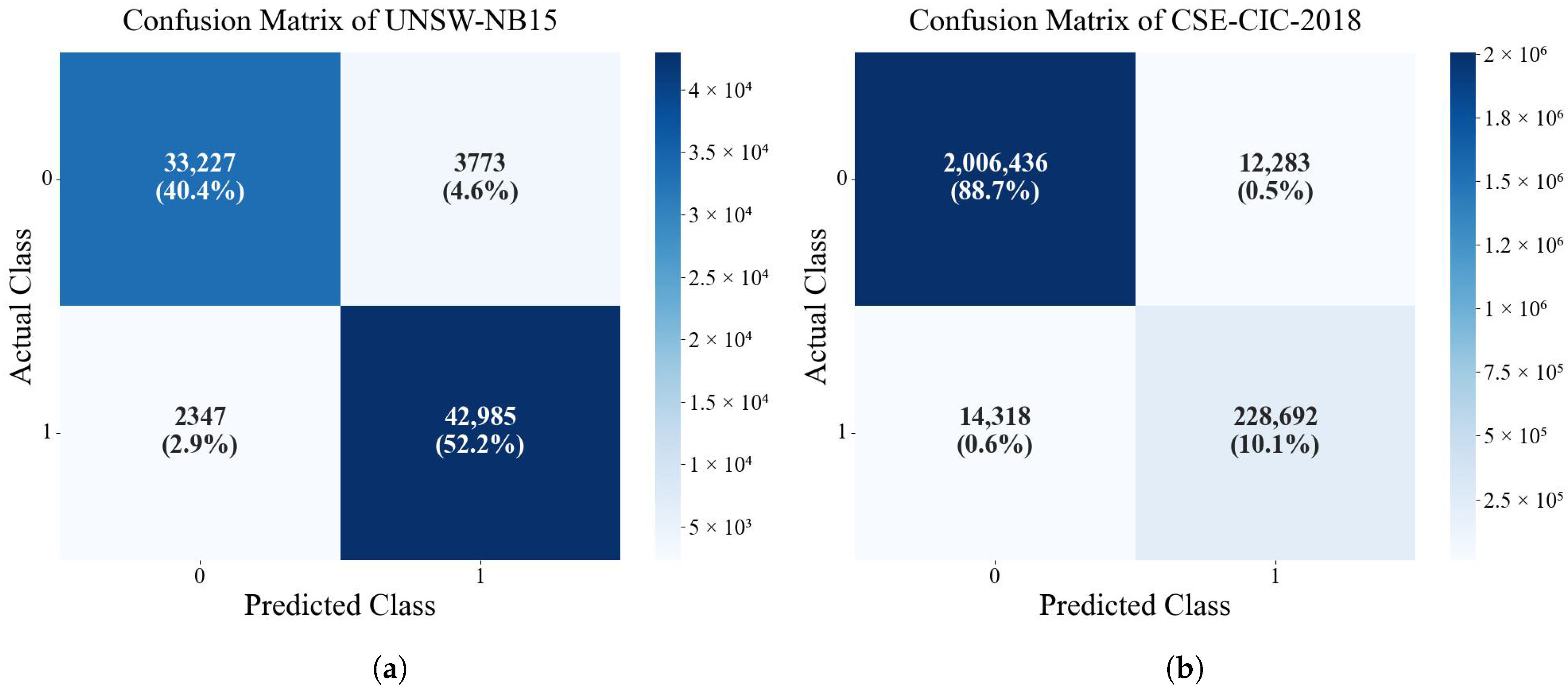
The confusion matrixes of tow datasets for the DyP-CNX approach are shown in Figure 4.

The confusion matrix results reveal that the model exhibits high overall classification performance on both datasets, but there are significant differences in the misclassification patterns. On the UNSW-NB15 dataset (Figure 4a), the model’s misclassification of the negative class (FN = 3773) is slightly higher than the misclassification of the positive class (FP = 2347), indicating that the model may lack sufficient sensitivity to certain attack types (such as low-frequency or novel attack patterns). On the CSE-CIC-IDS2018 dataset (Figure 4b), the misclassification of the positive class (FP = 14,318) is significantly higher than the misclassification of the negative class (FN = 12,283), suggesting that the model faces challenges in the specific identification of normal traffic, possibly due to the extremely large scale of normal traffic (TN = 2,006,436) in this dataset, leading the model to adopt a conservative decision threshold for attack behavior. This difference in misclassification patterns further reflects the model’s limited generalization to different network environments (UNSW-NB15 as a mixed traffic dataset, CSE-CIC-IDS2018 as a cloud platform traffic dataset). Specifically, the model’s capability to extract high-dimensional sparse features (such as encrypted traffic or low-frequency attacks in CSE-CIC-IDS2018) may be constrained by the CNN architecture, while XGBoost in the ensemble process may over-rely on explicit statistical features and fail to fully capture the temporal and contextual dependence characteristics of attack types. For further analysis, it is suggested to further breakdown the misclassification distribution by specific attack types (such as DoS, Exploit, etc.) to identify the model’s weak points for certain attacks (such as slow attacks or zero-day attacks).

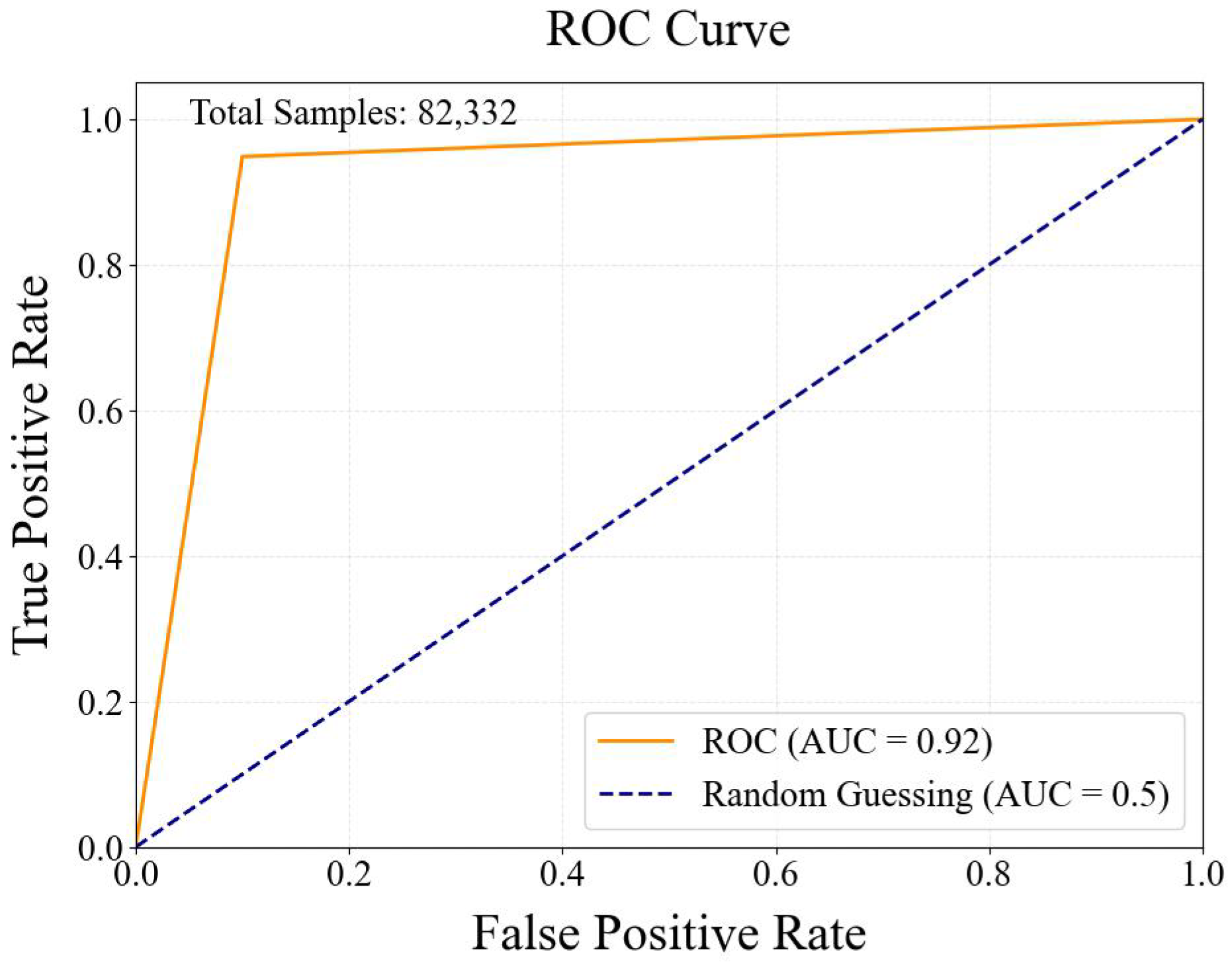
To further evaluate the classification performance of the method, the ROC curve is plotted to illustrate the relationship between the True Positive Rate (TPR) and the False Positive Rate (FPR), demonstrating the method’s performance at various threshold settings. The ROC curve of UNSW-NB15 is shown in Figure 5.

4.4.6. Comparisons Study

As shown in Table 11, this table demonstrates a comparison of different methods on the UNSW-NB15 dataset, primarily focusing on accuracy and F1 score metrics. AE-GRU [5] shows moderate performance in both metrics, indicating balanced performance. CL-FS [7] has slightly higher accuracy than AE-GRU but a lower F1 score, suggesting a trade-off between precision and recall. XGBoost-GRU [16] performs well in accuracy but has a lower F1 score, possibly indicating an imbalance between precision and recall. LightGBM [17] performs excellently in both metrics, demonstrating effective handling of data distribution and category prediction. SRF-CNN-BiLSTM [18] performs well, maintaining a good balance between accuracy and F1 score. Although DCNN-LSTM [27] has high accuracy, its lower F1 score indicates issues with class balance. Comparing the experimental results, it can be seen that the combination of GRU with boosting algorithms, as in AE-GRU and XGBoost-GRU, shows competitive performance but has not yet achieved the best results. The use of LSTM and CNN variants in DCNN-LSTM, despite high accuracy, shows challenges in some metrics.

As shown in Table 10, the experiment is based on the CSE-CIC-IDS 2018 dataset. This dataset originates from actual security projects and features high authenticity, diversity, and comprehensiveness. In particular, it performs well in simulating real-world environments, making its use for performance evaluation highly meaningful in practical applications. According to the results in Table 6, AI-AWS-RF [9], CLHF [28], and PCA-DNN [29] demonstrate stable performance with high accuracy and F1 scores, indicating good classification capabilities; the method proposed in this paper performs the best, achieving the highest accuracy and the highest F1 score. This clearly shows its advantages in classification accuracy and class balance.

As shown in Table 11, the XGBoost model exhibited relatively low performance, with an accuracy of 85.06%, a precision of 80.17%, and an F1 score of 87.71%. The standalone CNN model outperformed XGBoost, achieving an accuracy of 86.96%, a precision of 83.30%, and an F1 score of 88.97%. Our proposed method, DyP-CNX, which incorporates dynamic IQR normalization, demonstrated the best results, with an accuracy of 92.57%, a precision of 93.40%, and an F1 score of 91.57%. Compared to XGBoost, the standalone CNN improved accuracy by approximately 1 percentage point, indicating that deep learning models have a superior feature representation capability, enabling them to capture local features more effectively and, thus, enhance overall performance. However, combining dynamic normalization with DyP-CNX significantly increased performance, especially with about a 3-point improvement in the F1 score. This demonstrates that the deep fusion strategy employed in this paper—allowing the model to utilize both local and global features—further enhances the detection ability under complex and concealed attack scenarios, leading to improved performance.

Comparing Table 8 and Table 11, it can be observed that Ref. [16], which adds a GRU module to the XGBoost model in Table 11, achieves approximately a 2% improvement in accuracy and F1. The models SRFCNN-BiLSTM [18] and DCNN-LSTM [27] have also been somewhat optimized relative to the CNN in Table 11, with performance improvements to varying degrees. However, overall, their results are still inferior to the proposed DyP-CNX method. This further demonstrates that the DyP-CNX approach can effectively detect concealed threats in complex attack scenarios while avoiding over-sensitivity, providing a robust solution for practical network security defense.

In conclusion, DyP-CNX significantly outperforms other methods across all metrics, indicating its greater effectiveness in identifying and correctly classifying instances. While our model performs well on the specific dataset, it still has several limitations. Firstly, the model heavily relies on the representativeness of the training data; its performance may be affected when applied to different or more complex scenarios. Secondly, the deep model has high computational complexity, requiring substantial hardware resources during deployment, which may impact real-time performance and scalability. Additionally, the robustness of the model against unknown attack types or maliciously crafted adversarial samples needs further validation.

5. Conclusions

This paper proposes the hybrid architecture DyP-CNX, which achieves excellent results in network traffic detection. By introducing sliding window-based dynamic IQR normalization during data preprocessing, the approach effectively mitigates issues related to the temporal non-stationarity of data; combined with a random under-sampling strategy, it alleviates class imbalance. At the model level, the integration of CNN and XGBoost enables deep fusion of local features and global rules, enhancing detection performance. The experimental results demonstrate that this method achieves outstanding detection accuracy across multiple datasets, maintaining high precision while significantly reducing false alarms, thus reflecting its potential for application in complex network environments. However, considering the model’s complexity and hardware resource demands, its deployment in resource-constrained environments still faces challenges.

In future research, we will proceed from several aspects. First, we will further optimize the training time and architecture of the model to improve its performance. Second, we plan to introduce adversarial defense techniques and concept drift detection mechanisms to enhance the model’s adaptability and anti-interference capabilities in complex and changing environments, ensuring its reliability in practical applications.

References

1. Pavithra, S.; Vikas, K.V. Detecting Unbalanced Network Traffic Intrusions with Deep Learning. IEEE Access 2024, 12, 74096–74107. [Google Scholar] [CrossRef]
2. Liao, H.-J.; Lin, C.-H.R.; Lin, Y.-C.; Tung, K.-Y. Intrusion Detection System: A Comprehensive Review. J. NetWork. Comput. Appl. 2013, 36, 16–24. [Google Scholar] [CrossRef]
3. Ahmad, Z.; Khan, A.S. Deep Learning for Intrusion Detection Systems: Challenges and Future Directions. In Proceedings of the IEEE Symposium on Security and Privacy, San Francisco, CA, USA, 23–25 May 2022; pp. 123–140. [Google Scholar]
4. Barkah, A.; Selamat, S.; Abidin, Z.; Wahyudi, R. Impact of Data Balancing and Feature Selection on Machine Learning-based Network Intrusion Detection. JOIV Int. J. Inform. Vis. 2023, 7, 241–248. [Google Scholar] [CrossRef]
5. Mushtaq, E.; Zameer, A.; Nasir, R. Knacks of a hybrid anomaly detection model using deep auto-encoder driven gated recurrent unit. Comput. Netw. 2023, 226, 109681. [Google Scholar] [CrossRef]
6. Park, C.; Lee, J.; Kim, Y.; Park, J.-G.; Kim, H.; Hong, D. An Enhanced AI-Based Network Intrusion Detection System Using Generative Adversarial Networks. IEEE Internet Things J. 2023, 10, 2330–2345. [Google Scholar] [CrossRef]
7. Chen, H.; Cheng, M.; Jin, H.; Wu, C.; Jiang, C. An Intrusion Detection Model Integrating Contrastive Learning and Feature Selection. Inf. Secur. Res. 2024, 10, 453–461. [Google Scholar]
8. Zhou, S.; Che, S.; Kao, Y.; Zhang, X.; Guo, S. Network Intrusion Detection Based on Feature Selection and Spatiotemporal Features. Comput. Eng. 2024, 51, 223–231. [Google Scholar]
9. Chopra, S.; Sreedevi, A.G. Scrutinization of Threats from a Cloud-based Network Traffic Environment. In Proceedings of the 2024 11th International Conference on Computing for Sustainable Global Development (INDIACom), New Delhi, India, 28 February–1 March 2024; pp. 377–383. [Google Scholar]
10. Pratomo, B.A.; Burnap, P.; Theodorakopoulos, G. Unsupervised Approach for Detecting Low Rate Attacks on Network Traffic with Autoencoder. In Proceedings of the 2018 International Conference on Cyber Security and Protection of Digital Services (Cyber Security), Glasgow, UK, 11–12 June 2018; pp. 1–8. [Google Scholar]
11. Sinha, A.; Verma, J.; Alkhayyat, A.; Mahmood, H.R.; Ahmed, S.; Symbiosis, S.G. Accurate and Flexible Malware Detection in Cloud Environments with a Z-Score Based CSOM Model. In Proceedings of the 2025 4th International Conference on Computing and Information Technology (ICCIT), Tabuk, Saudi Arabia, 16–17 April 2025; pp. 598–603. [Google Scholar] [CrossRef]
12. Hassan, M.; Metwally, K.; Elshafey, M.A. ZF-DDOS: An Enhanced Statistical-Based DDoS Detection Approach using Integrated Z-Score and Fast-Entropy Measures. In Proceedings of the 2024 6th International Conference on Computing and Informatics (ICCI), Cairo, Egypt, 6–7 March 2024; pp. 145–152. [Google Scholar] [CrossRef]
13. Kotenko, I.; Saenko, I.; Kribel, A.; Lauta, O. A technique for early detection of cyberattacks using the traffic self-similarity property and a statistical approach. In Proceedings of the 2021 29th Euromicro International Conference on Parallel, Distributed and Network-Based Processing (PDP), Valladolid, Spain, 10–12 March 2021; pp. 281–284. [Google Scholar] [CrossRef]
14. Jayaprakash, J.S.; Kodati, S.; Kanchana, A.; Al-Farouni, M.; Ramachandra, A.C. An Effective Cyber Security Threat Detection in Smart Cities Using Dueling Deep Q Networks. In Proceedings of the 2024 4th International Conference on Mobile Networks and Wireless Communications (ICMNWC), Tumkuru, India, 4–5 December 2024; pp. 1–5. [Google Scholar] [CrossRef]
15. Miah, M.O.; Khan, S.S.; Shatabda, S.; Farid, D.M. Improving Detection Accuracy for Imbalanced Network Intrusion Classification using Cluster-based Under-sampling with Random Forests. In Proceedings of the 2019 1st International Conference on Advances in Science, Engineering and Robotics Technology (ICASERT), Dhaka, Bangladesh, 3–5 May 2019; pp. 1–5. [Google Scholar] [CrossRef]
16. Guo, Y.; Chen, M.; Yuan, C.; Zheng, F. Research on Campus Network Security Situational Awareness Technology Based on XGBoost Machine Learning. In Proceedings of the 2024 5th International Conference on Big Data & Artificial Intelligence & Software Engineering (ICBASE), Wenzhou, China, 20–22 September 2024; pp. 948–952. [Google Scholar]
17. Vallabhapurapu, L.S.R.; Suripeddi, S.; Unguturi, S.C.; Singh, V.K. Hybrid Feature Selection for Effective Intrusion Detection. In Proceedings of the 2024 Second International Conference on Emerging Trends in Information Technology and Engineering (ICETITE), Vellore, India, 22–23 February 2024; pp. 1–6. [Google Scholar]
18. Chen, H.; You, Y.; Jin, H.; Wu, C.; Zou, J. An Intrusion Detection Method Combining Improved Sampling Technology and SRFCNN-BiLSTM. Comput. Eng. Appl. 2024, 9, 315–324. [Google Scholar]
19. Devi, R.; Kumar, A.; Kumar, V.; Saini, A.; Kumari, A.; Kumar, V. A Review Paper on IDS in Edge Computing or EoT. In Proceedings of the 2022 International Conference on Fourth Industrial Revolution Based Technology and Practices (ICFIRTP), Uttarakhand, India, 23–24 November 2022; pp. 30–35. [Google Scholar]
20. Deng, J.; Cheng, L.; Yuan, H.; Zheng, K.; Li, X.; Li, Q. An Online Detection System for LDoS attack Based on XGBoost. In Proceedings of the 2023 IEEE International Conference on Parallel & Distributed Processing with Applications, Big Data & Cloud Computing, Sustainable Computing & Communications, Social Computing & Networking (ISPA/BDCloud/SocialCom/SustainCom), Wuhan, China, 21–24 December 2023; pp. 1083–1088. [Google Scholar]
21. Dahouda, M.K.; Joe, I. A Deep-Learned Embedding Technique for Categorical Features Encoding. IEEE Access 2021, 9, 114381–114391. [Google Scholar] [CrossRef]
22. Bai, K.; Dai, S.; Zhang, Z.; Jin, S. Well Leakage Prediction Using Swarm Intelligence Algo-rithm-Optimized Improved Random Forest Algorithm. Mod. Electron. Tech. 2025, 48, 159–168. [Google Scholar]
23. Yoo, S.; Kim, S.; Jang, Y. Two-Level Transfer Functions Using t-SNE for Data Segmentation in Direct Volume Rendering. IEEE Trans. Vis. Comput. Graph. 2025, 31, 5948–5961. [Google Scholar] [CrossRef] [PubMed]
24. Moustafa, N.; Slay, J. UNSW-NB15: A Comprehensive Data Set for Network Intrusion Detection Systems (UNSW-NB15 Network Data Set); IEEE: New York, NY, USA, 2015. [Google Scholar]
25. Sharafaldin, I.; Lashkari, A.H.; Ghorbani, A.A. Toward Generating a New Intrusion Detection Dataset and Intrusion Traffic Characterization. In Proceedings of the 4th International Conference on Information Systems Security and Privacy (ICISSP), Funchal, Portugal, 22–24 January 2018. [Google Scholar]
26. Zhang, K.; Su, H.; Dou, Y. A New Accuracy Evaluation Method for Multi-classification Tasks Based on Confusion Matrix. Comput. Eng. Sci. 2021, 43, 1910–1919. [Google Scholar]
27. Gao, Z.; Li, A. Research on Malicious Traffic Detection Technology Based on Deep Learning. In Proceedings of the 2024 2nd International Conference on Signal Processing and Intelligent Computing (SPIC), Guangzhou, China, 20–22 September 2024; pp. 283–287. [Google Scholar] [CrossRef]
28. Alzubi, J.A.; Alzubi, O.A.; Qiqieh, I.; Singh, A. A Blended Deep Learning Intrusion Detection Framework for Consuma-ble Edge-Centric IoMT Industry. IEEE Trans. Consum. Electron. 2024, 70, 2049–2057. [Google Scholar] [CrossRef]
29. Al-Fawa’reh, M.; Al-Fayoumi, M.; Nashwan, S.; Fraihat, S. Cyber threat intelligence using PCA-DNN model to detect abnormal network behavior. Egypt. Inform. J. 2022, 23, 173–185. [Google Scholar] [CrossRef]
Figure 1. The proposed model.
Applsci 15 09431 g001
Figure 2. CNN training loss curve.
Applsci 15 09431 g002
Figure 3. Comparison before and after data preprocessing. The panels show (a) the original data distribution and (b) the distribution following preprocessing.
Applsci 15 09431 g003
Figure 4. Confusion matrix based on different datasets. The panels show (a) the confusion matrix based on the UNSW-NB15 dataset and (b) the confusion matrix based on the CSE-CIC-IDS 2018 dataset.
Applsci 15 09431 g004
Figure 5. ROC curve.
Applsci 15 09431 g005